On Nonlocal Gross-Pitaevskii Equations with Periodic Potentials
Abstract
The Gross-Pitaevskii equation is a widely used model in physics, in particular in the context of Bose-Einstein condensates. However, it only takes into account local interactions between particles. This paper demonstrates the validity of using a nonlocal formulation as a generalization of the local model. In particular, the paper demonstrates that the solution of the nonlocal model approaches in norm the solution of the local model as the nonlocal model approaches the local model. The nonlocality and potential used for the Gross-Pitaevskii equation are quite general, thus this paper shows that one can easily add nonlocal effects to interesting classes of Bose-Einstein condensate models. Based on a particular choice of potential for the nonlocal Gross-Pitaevskii equation, we establish the orbital stability of a class of parameter-dependent solutions to the nonlocal problem for certain parameter regimes. Numerical results corroborate the analytical stability results and lead to predictions about the stability of the class of solutions for parameter values outside of the purview of the theory established in this paper.
I Introduction
The last 15 years has a seen a rapid growth in interest concerning the modeling of Bose-Einstein condensates. The body of literature concerning this subject is too vast to consider here, but a simplified description of the field would include the study of the Gross-Pitaevskii equation
| (1) |
where , with corresponding to repulsive interactions between particles in the condensate, and corresponding to attractive interactions. The function represents an approximation to the wave function used to describe the probability density for the location of particles in the condensate.
The validity of this equation as an approximation to the many-particle formulation of the problem has been established in lieb . However, an assumption of a pairwise -function interaction among particles is used to derive (1). This clearly cannot capture all of the physics in the problem since each particle in the condensate exerts forces that act at a distance. Thus the next order of approximation to the many-particle formulation would be to include a more general interaction potential simulating nonlocal interactions between particles. This is done in decon by studying the modified one-dimensional Gross-Pitaevskii equation
| (2) |
where , and , with being a positive, even function such that
in the sense of distributions. In decon , is called the nonlocality parameter. The authors of decon assume that the condensate is trapped in both a harmonic confining potential and an external standing-wave potential. While in decon a three-dimensional version of (2) is derived, the presence of the standing-wave potential allows the reduction to a one-dimensional model (cf. olshan ).
Nonlocal models like (2) are also called Hartree-Fock equations. These have been extensively studied in the case that , i.e. in modeling Coulombic interactions between particles (cf. gini , hart ). Recent literature on the formation of dipolar condensates has introduced nonsingular nonlocalities characterized by cubic decay (cf. sinha , kevre ). These nonlocalities with cubic decay fit into the class studied in this paper. Other models with a varying nonlocality parameter have appeared in the optics literature trillo . The analysis of the well-posedness and convergence of nonlocal, nonlinear Schrödinger type models to local ones can be found in cao1 and cao2 , though the models examined in those papers are different from those studied in this paper.
The authors of decon , working with the potential , derived the traveling-wave solutions
| (3) |
where
with a constant called the offset size. Defining , the traveling-wave solution can be rewritten as
which shows the spatial component of (3) is periodic with period . The coefficients appearing in must satisfy the restrictions
Setting and equal to one, and taking , which in decon is described as large, and , the authors of decon study the stability of (3) by numerical simulations using and . The authors report results which numerically demonstrate that for the local case, i.e. when , (3) is stable with respect to perturbations due to roundoff error in the numerical simulation. However, their results also suggest that (3) is unstable when the nonlocality parameter is positive, and that the instability emerges at a fixed time in their simulations, independent of the value of . The authors of decon also study the effect of changing the convolution kernel, and they report that the results are similar to those for the case .
It is conjectured in decon that a beyond-all-orders phenomena may be responsible for the behavior exhibited in their numerics. As pointed out in decon , if the behavior exhibited in their numerics is accurate and truly independent of the choice of interaction potential, then (2) cannot be viewed as a valid generalization of (1). That is to say, no matter how small one makes the nonlocal interaction term, the results of decon seem to imply that one cannot approach the local behavior. This is described as a lack of asymptotic equivalence of stability (AES) in decon .
The purpose of this paper is to address both the issue of whether or not (2) is AES to (1) and under what conditions (3) is a stable solution of Equation (2). To do this, we first fix some notation and introduce the spaces in which we work. Let denote the circle of circumference . Introduce the space which is the completion of the continuous -periodic functions in the norm
In practice the integral could be evaluated over any interval of width since is a -periodic function. Note, throughout the remainder of the text is abbreviated by . We define the norm, denoted as , of the product space , via
For operators that map to itself, we denote the norm of via
The norms are defined in an identical way. The Sobolev spaces are defined as follows:
where
and the terms come from the Fourier series of , which is
where
| (4) |
and
where denotes the complex conjugate of . The product space is denoted by . Finally, define the Fourier transform of , say , by
To address the issue of AES, we first prove the local-well posedness, in for , and global-well posedness of (2) over the space based on the following assumptions.
-
:
The potential is a smooth, -periodic function,
-
:
,
-
:
with ,
-
:
, and
-
:
, where .
Note that the maximum of could be chosen larger than one without affecting our results. We make this choice in order for a cleaner presentation. Using the local and global-well posedness results, we prove
Theorem 1.
Let . Assuming the hypotheses , choose constant such that for where is an initial condition for (2) and is an initial condition for (1). Let in the norm as . Let and be the unique T-periodic solutions to (1) and (2) respectively for the given initial conditions. Then there exists a constant and a function , where for , such that, for any finite , we have the bound
for .
Thus, on any finite interval of time, as one lets the nonlocality parameter approach zero, the solution to (2) converges uniformly in space to the solution of (1). This shows that AES is a common feature for a large class of potentials and nonlocal, repulsive interactions. Therefore the results in decon are likely due to artifacts of their numerical computations, as opposed to being inherent to the equation.
As to the stability of (3), we first need to define the notion of stability to be established (cf. gss ). Let denote a solution to either (1) or (2) with initial condition . Writing (3) as , we say that is orbitally stable in , if for any , there is a such that if then
The other notion of stability we use is that of spectral stability. First, separate (1) or (2) into real and imaginary parts. Denote the linearization of either of these systems around (3) as . Using the scaling , has terms that are -periodic functions. Let denote the spectrum of computed over the space , . In effect, we are computing the impact of perturbing (3) by -periodic perturbations, or -periodic perturbations in the unscaled coordinate. We say (3) is spectrally stable if for , . Note, more details are provided in Section 3. Also, given that the nonlinear problem is Hamiltonian, the condition of spectral stability reduces to having spectrum only on the imaginary line, i.e. . With these definitions in hand, we prove the following three theorems. Throughout these remaining theorems we assume that
-
:
,
-
:
, is even, and ,
-
:
, and
-
:
, with .
Theorem 2.
Let . Assuming the Hypotheses , for any values of and the nonlocality parameter , and for perturbations of period , where , the solution (3) is spectrally stable for sufficiently large offset size , , and sufficiently small.
Theorem 3.
Theorem 4.
Let . Assuming the Hypotheses , with , if , then for offset size and sufficiently small, (3) is spectrally unstable with respect to perturbations of period , where .
The content of these three theorems shows that the role of a small nonlocality parameter is dependent upon the other parameters in the problem, particularly the offset size . Theorems 2 and 3 are proven by showing that if is sufficiently large, then the operator is positive semi-definite. Then, using Krein signature arguments found in hara , we get both spectral and orbital stability. Thus, introducing small nonlocality should not effect the stability of (3), while Theorem 4 shows that if is too small, then even removing the nonlocality parameter does not stabilize the solution. In contrast, as is shown later, we can always get a spectrally stable problem by letting for any choice of the other parameters. Thus it appears that while a small amount of nonlocality does not affect stability, large amounts do.
The above theorems do not allow for arbitrary choices of parameters since each theorem requires to be small, which ensures that remains positive semi-definite. We cannot at this time provide explicit bounds on how large can be such that Theorems 2 and 3 remain true since we cannot control the spectra of for . Therefore, we must treat the parameter values used in decon as outside the scope of what is proved in this paper. We provide numerical experiments in order to make conjectures about the stability of (3). First, we use the above theorems to calibrate our numerics by picking parameter values that can reasonably be believed to satisfy the constraints of Theorems 3 and 4. Our numerics behave as the theory predicts. Second, we present numerical experiments using the parameter values found in decon , and from this we conjecture that in fact (3) should be stable for the parameter values chosen. As mentioned above, these are , , , and .
As in decon , a pseudo-spectral method is used for the spatial variable, while a standard Runge-Kutta method is used for time evolution. The most likely explanation for the discrepancy between the results reported here and those of decon is the way in which the convolution is handled. In this paper, no approximation is made in the integral or to the convolution kernel. However, in decon , it appears an approximation is made to the kernel which introduces an error that appears difficult for the pseudo-spectral method to resolve. In private communications, the authors of decon have been made aware of these discrepancies. They have encouraged the explanation for them in this manuscript.
The structure of the paper is as follows. In Section 2, we present the proof of the AES of (1) and (2). In Section 3, we find the linearization around (3), and we establish some basic results about the convolution kernel that are used later. In Section 4, Theorems 2 and 3 are proved, while in Section 5, Theorem 4 is proved. Finally, Section 6 presents the numerical results.
II Asymptotic Equivalence of Stability
We proceed in the following fashion. In order to make the presentation self-contained, we first establish the local-in-time well-posedness of the nonlocal Gross-Pitaevskii equation from which we obtain a local-in-time form of AES. We then establish the continuity in of solutions to (2). Finally, we establish the global-in-time well posedness of (2) which allows us to prove Theorem 1. Note, we use Hypotheses throughout the remainder of the section.
We begin by establishing some basic lemmas concerning the convolution kernel . We show, using the assumptions stated for Theorem 1, that the Fourier transform of the convolution kernel is Lipschitz continuous in .
Lemma 1.
One has
Proof.
With
we have
Using the Mean-Value Theorem, one gets
Thus the result is shown. Using Hypothesis , which amounts to assuming , we also have that the bound is meaningful. ∎
Let . We then show
Lemma 2.
Given Hypotheses and , for ,
Proof.
First we note that
since for
, and by Hypothesis . By Hypothesis , , and by a corollary to the Dominated Convergence Theorem (foll , Theorem 2.25) one has
or
and the result is shown. ∎
From the previous lemma, one gets
Lemma 3.
Let . One has that
Proof.
II.1 Local-in-Time Well Posedness of the Nonlocal Gross-Pitaevskii Equation and a Weak AES Theorem
For the small-time argument, with initial condition , we rewrite (2) in the Duhamel form
| (6) |
where , with assumed to be, by Hypothesis , a smooth -periodic function. As for controlling , since the operator is skew-adjoint, by Stone’s theorem eng , is a unitary operator from to itself. One also has that
where denotes the symbol of . Since is self-adjoint, is strictly real, and so one has the bound
since for all .
Throughout the remainder of the section, we assume is acting on the space where . Using Lemma 3, and defining by,
one has for
We then choose constant such that
for , with independent of . We define the metric space , for , by
where
The map takes to for . It is straightforward to show, again using Lemma 3, that is a contraction for , and therefore, using the Banach Fixed Point Theorem tao , one has local well posedness for initial condition , , on the space for
From the local well-posedness result, we now prove
Lemma 4.
One has that , , and are continuous functions of time for . Further, the Fourier coefficients of and are continuous functions of time for .
Proof.
Let , and . Letting denote the solution for initial condition , we have
where
For the first term, we have that
Using the Dominated Convergence Theorem shows that this term then vanishes as or vice versa. The local well posedness result and Lemma 3 ensures that
so we have
Using a dominated convergence argument shows that the remaining term must also vanish as . Thus we have shown that is a continuous function in for . By a Sobolev embedding foll , we also have that is continuous in and bounded above by . Given that
we then see that is continuous as well. This result then immediately gives that the Fourier coefficients of and are also continuous in time since
for . The case is treated identically, so the result is proved. ∎
Taking and to be nonnegative, we now choose the initial conditions to be continuous in with respect to the -norm, i.e.
| (7) |
We then prove
Lemma 5.
For , , and , if the initial condition is continuous in with respect to the -norm, the solution is continuous in with respect to the -norm, i.e.
Proof.
Choosing , one has that
In the last term of the above inequality, the convolutions depend on the different values of . Thus
For , using the local-in-time well posedness result, the following inequality
holds. To control the last term in this inequality, set (as in Lemma 3)
from which one gets that
From the local-in-time well posedness result
so that using Lemma 1, one gets the pointwise estimate
where the index is arbitrary. Using Hypothesis , is uniformly bounded in , so the terms
are uniformly bounded for all . Using the Dominated Convergence Theorem, one sees that
| (8) |
Then
where
with
The term vanishes as by assumption (see (7)). Further, since, as shown in Lemma 4, the coefficients are continuous in time, this makes the term continuous in time since it is a uniform sum of continuous functions. Thus, the supremum is attained at some time , and since (8) holds for any , one has that
where . Therefore,
We know from Lemma 4 that is a continuous function in for . Using Gronwall’s inequality tao , one gets
and the result is therefore proved. ∎
Since , it follows that
and thus
Therefore the lemma establishes that (2) is local in time AES to (1). Further, once a global-in-time well posedness result holds for (2) (which amounts to establishing a uniform bound on for all time), the above lemma immediately furnishes a global in time AES result.
II.2 Global-in-Time Well Posedness and the AES Theorem
As established in decon , (2) has at least two conserved quantities: the norm and the Hamiltonian
We choose . Following the argument in linar , with positive by Hypothesis , , and a solution to (2) on time interval , with initial condition , then one has that
Using Young’s inequality, one has
Thus the assumptions guarantee that . Since the norm is also conserved, there exists a constant such that
| (9) |
This bound is independent of . If we now try to iterate our local-in-time well posedness argument onto a time interval , where is chosen so that the intervals and overlap, then for the new interval we may let take the role of the value . We must work on a ball with and
Since the inequality (9) is independent of time, one can repeat the derivation of (9) on the time interval and obtain the same bound. Thus one can iterate the local argument such that the value of need not increase, and thus the width of the new intervals can be set to a fixed value. This establishes for the repulsive case a global existence of solutions to (2) in for . As argued above, one can immediately extend the argument in Lemma 5 so that one has a global AES theorem.
III Stability: The Linearization and Its Properties
Having established Theorem 1, we turn to analyzing the stability of (3). Note, throughout the remainder of the paper we assume Hypotheses as listed in the Introduction. Writing (3) as , and introducing the transformation , we see that is a stationary solution of the equation
| (10) |
With , we rewrite (10) as
| (11) |
where
and . Note, (11) is posed over , but the global-well posedness result established in the last section carries over without issue. We set from Hypothesis . Letting
and equating and , and collecting all terms, we get the linearized system
With , we have
Thus, since is an even function by Hypothesis , we write
and we have, for ,
Introducing the transformation , so that the potential and (3) are now -periodic functions, and defining
we rewrite the linearized system with as
where . Defining
and letting
| (12) |
we can rewrite the linearized system as
with the operator given by
Using separation of variables, i.e. and , formally gives us an eigenvalue problem. We now study the spectrum of over . Note, the fact we are working over the space reflects the fact that we have separated the perturbations of the exact solution into real and imaginary parts.
III.1 The Eigenvalue Problem on
We wish to solve the spectral problem
where . As will be shown after this section, the operator on the domain has a compact resolvent operator. Therefore the spectrum, , of the operator is discrete, and solving the eigenvalue problem is sufficient to determine the spectrum. To find the spectrum of , we note that an arbitrary -periodic function, , can be decomposed as
where is a -periodic function, and . Therefore, one can apply a similar decomposition to and so that
One can show, for real , that
where the operator is given by
with
and
Here
Thus one has for any eigenvalue that
The term is a periodic function. Since none of the functions share a common period shorter than , the equality
must hold for each value of . This shows that one can decompose the spectrum of on as a union of the spectra of the operators posed on , i.e. one can write
Note, one cannot rely on standard Floquet theory since the spectral problem is not an ordinary differential equation. In the succeeding sections we study the problem on , with , in order to deal with arbitrary values of .
III.2 Basic Results about the Convolution Kernel and Linearization
We prove a number of technical lemmas concerning the convolution and linearization that are used throughout the remainder of the paper.
Lemma 6.
Given Hypotheses and , the operator is compact. Further, is continuous in , , with respect to the -norm.
Proof.
Using the same arguments as in Lemma 2, one finds the Fourier series representation of , which we denote as , as
where is diagonal and . Since in Hypothesis we assume , by the Riemann-Lebesgue lemma foll , we have
Defining
we see that for
Since we assume in Hypothesis that , the above sum decays to zero as , and the operator is a uniform limit of finite rank operators. Therefore, so is , and must then be compact.
To prove the last part of the lemma, we note that for
so using Hypothesis and the Dominated Convergence Theorem shows that as , or is continuous in . Likewise, we have, using Hypothesis ,
where
For , one has
so using a dominated convergence argument, one gets as . Thus as , so is continuous in . ∎
From the previous lemma one gets
Lemma 7.
The operator has a compact resolvent on .
Proof.
Given that , where
one has that , where we have suppressed the dependence on and , is compact since it is the product of bounded and compact operators. Further, a straightforward application of Fourier series shows that has compact resolvent on . Let be a complex number with nonzero imaginary part. Then
| (13) |
The operator is Fredholm since is compact. The right-hand side of (13) has a trivial kernel since is self-adjoint. Thus the left-hand side of (13) also has a trivial kernel, which implies that has a bounded inverse lax . Therefore, from
one sees that is the product of a bounded and a compact operator, and is therefore itself compact. ∎
Assuming that is in the resolvent of , and using that
where is in the resolvent of , one sees that has a compact resolvent on since is the product of compact and bounded operators.
We now need to establish some limiting behavior of the operator as the nonlocality parameter becomes large. We prove:
Lemma 8.
Given Hypothesis , for ,
Proof.
One has
Examining the norm of the operator , one gets
Note, the sum is convergent by Hypothesis . For a given value of the nonlocality parameter and an arbitrarily chosen value of , choose such that
Next, choose large enough such that
The second assumption does not alter the first since choosing a large value corresponds to choosing a larger value of . Thus, for ,
and uniformly in norm as . ∎
We finally prove that the resolvents of and converge in the -norm. This is used to show, in effect, that the spectra of one operator is a perturbation in of the other.
Lemma 9.
Suppose there exists such that is in the resolvent of for . Further suppose that exists. Then converges to in the -norm as .
Proof.
Define the operator . Then we have that
We have that
where , and and are such that . Using the fact that and are bounded in and Lemma 6,
Defining , we rewrite so that
We then get that
where . The operator is a constant coefficient operator. Thus, using the Fourier transform, it is straightforward to show it is bounded and must vanish in the -norm as . Thus we have that
Taking sufficiently small so that , we have that
which shows that
∎
IV Stability for Small Potential and Large Offset Size
IV.1 Computation of the Spectrum with
In this section, we compute the spectrum of over , with or (see (12)). As explained earlier, this is done by computing the spectrum of the operators over , . To do this, we notice that we can treat as a constant coefficient operator with a compact perturbation. For the remainder of the section, we assume so that the compact perturbation decays uniformly to zero as . The case is covered by noting that is a relatively compact perturbation of , which we note was used to prove Lemma 9. Therefore one can find the eigenvalues of by taking limits of the eigenvalues of .
Using the Fourier transform, we compute the spectrum and eigenfunctions of explicitly. One has
and for , the corresponding eigenfunctions for the eigenvalues on the positive imaginary axis are
| (14) |
while for ,
| (15) |
Taking conjugates and letting gives the corresponding eigenfunctions for the eigenvalues on the negative imaginary axis.
The eigenvalue problem for the operator and eigenvalue is of course to find nontrivial such that
We write, as in Lemma 7,
and let , where is an eigenvalue of , and is a perturbation of that will be determined exactly. We have
| (16) |
Let
and
Define to be the projection onto the null space of . Since is self adjoint, we use a Lyupanov-Schmidt reduction hale to rewrite (16) as
| (17) | |||||
| (18) |
where , is in the null space of , and
At this point, the equations (17) and (18) are the same as the original eigenvalue problem. No added assumptions or constraints have been made. Therefore solving (17) and (18) is equivalent to solving the original eigenvalue problem.
Rewriting (17) as
we may formally write
Though this expansion is valid for sufficiently large (see Lemma 8), it is more important as a motivation to look at the terms . For example, let or , with on the positive imaginary axis, so that is given by (15). For ,
so that
where
and
Note, we suppress the parameters and in for the sake of clarity in the presentation. Thus , and
Hence, for ,
and for ,
We consider for or . We see that
and hence for , we obtain
For , we have
Define the constants and such that and . Therefore, equating
gives a solution of (17).
Using (18), one obtains
From the work above, since , we see this reduces to
Writing
where and , we see that we want to solve the quadratic equation
| (19) |
Let , where and are real values. Therefore, by separating into real and imaginary parts, (19) becomes
If we assume , we have , which implies
The right-hand side of the above expression is always negative by construction, since . Thus , so that . Therefore we have
Since we know, as shown in Lemma 8, that as , and we need as , this determines the correct sign when solving the quadratic equation in . With this choice of , we see , so , and the choice of is well defined.
For the case that or , proceeding in a fashion identical to that above, one shows that
and
Here
and
where .
We again equate , which solves (17), and from (18) one gets a characteristic equation for which is
Finally,
Given that the operator is not symmetric with respect to conjugation followed by equating to , we must repeat the above computations except now with the expansions around the eigenvalues along the negative imaginary axis. The process is identical to that above, and we only list the results. For or , we have
where is given by
The corresponding eigenfunctions are
where and .
Likewise, for , we have
with . The corresponding eigenfunctions are
with and .
The only issue remaining is whether we have captured the entire spectrum of for each value of . However, every eigenvalue is a perturbation of an eigenvalue in the constant coefficient case, which has only simple eigenvalues in its spectrum since is a skew-adjoint operator with compact resolvent. Hence we have not missed any eigenvalues due to multiplicity. Thus we have computed for .
IV.2 Krein Signature
For a purely imaginary semisimple eigenvalue with eigenvector , the Krein signature of is defined as bjorn . Let
which, for the eigenvalues that represent perturbations of eigenvalues on the positive imaginary axis, is given by
where the in corresponds to choosing and the corresponds to . A similar expression can be derived for the eigenvalues starting on the negative imaginary axis.
Given the definition for , it is straightforward to show for and , that
| (20) | |||||
Along the positive imaginary axis, one again lets the of correspond to the case , while we take for . This relationship is reversed on the negative imaginary axis. Thus we see, starting on the positive imaginary axis, for , , , or , all the terms in (20) are positive. For or , we note that , thus
which is positive for or , .
Likewise, along the negative imaginary axis, for , , , or , all terms are positive. For or , we have
so that the eigenvalues corresponding to and on the negative imaginary axis have positive Krein signature.
However, for or on either part of the imaginary axis, if we let , . Therefore we see that for sufficiently small , with all other parameters fixed, the eigenvalues for or have negative Krein signature. On the other hand, fixing all other parameters except , if we allow the offset size to become arbitrarily large, then and
| (21) |
Hence it is possible for eigenvalues to pass through the origin or switch Krein signature.
Being more careful, we focus on the eigenvalues with potentially negative Krein signature, which are
and
One sees that for given and , one can find a sufficiently large value of such that none of these four eigenvalues pass through the origin for . Noting that by Hypothesis , and since is continuous in (see Lemma 6), we define . We define the parameter to be
If , then all four eigenvalues cannot pass through the origin for . Setting , one has from (21) that each of the four eigenvalues must have positive Krein signature for .
We now apply a theorem of hara which states that
| (22) |
where is the number of eigenvalues of on the positive real axis, is the number of eigenvalues with real part, is the number of imaginary eigenvalues with negative Krein signature, and is the number of negative eigenvalues of . In order to apply this theorem, one needs to show that the operator satisfies Assumptions in hara . Given that , where is compact, and that the reciprocals of the eigenvalues of are square summable, then showing all four assumptions hold for is straightforward. For , , and thus . Since the operator remains invertible for , which means no eigenvalue passes through the origin, then for . This establishes that every eigenvalue of has positive Krein signature.
IV.3 Spectral and Orbital Stability for Small Potential Height
As shown above, for sufficiently large, , and , there are no eigenvalues of negative Krein signature, which by (22) implies that the operator is positive definite. Thus a standard perturbation argument guarantees that for small enough , no eigenvalue of crosses through the origin, and thus we must have . Using (22) again shows that (3) is spectrally stable for a given with sufficiently small potential height.
In the case that , , one has by continuity of the spectrum with respect to the parameter that every eigenvalue of must be on the imaginary axis. However, for any value of , there is an eigenvalue at the origin, with eigenvector
due to the phase symmetry which generates (3). Thus (22) cannot be applied. Likewise, there is a generalized eigenvector of at the origin,
Using the work above, one formally sees that the eigenvalues at the origin correspond to the eigenvalues and colliding at the origin for . We now prove that the generalized kernel of consists only of and . First define the projection operator (kato ,Theorem 6.17)
where is a closed, bounded contour in the complex plane such that and the origin is inside . We further suppose that and are the only eigenvalues of inside for sufficiently small. Since has a compact resolvent, it has discrete eigenvalues that accumulate only at infinity. Therefore, we can also choose such that and so that contains only a finite, counting multiplicity, number of the eigenvalues of . Thus the projection is well-defined and finite-dimensional. We then have
Since is continuous in , on , which is compact, the supremum is attained. We further restrict such that . Using Lemma 9 then gives
Since and are projection operators, we then have (kato , pg. 156) that
where denotes the range of . By construction , and thus . The dimension of counts the algebraic multiplicity of an eigenvalue (see kato , pg. 181), and so we see that the generalized kernel of can only consist of and .
Since is self adjoint and has a compact resolvent (see Lemma 7), it cannot have a generalized eigenvalue at the origin for any . At (i.e. ), it is straightforward to show that
Thus, for and , the operator has a simple eigenvalue at the origin and otherwise has only positive eigenvalues. Since the eigenvector at the origin persists for any , every nonzero eigenvalue of remains positive for small values of . This implies that for and sufficiently small. If , one concludes spectral stability for small potential height by way of the following argument. If , , then
and since is not in the kernel of by assumption. is strictly imaginary and nonzero. Thus is strictly imaginary. We have now shown that the spectrum of on , which is decomposed as
is strictly imaginary for small potential height since is strictly imaginary and there are a finite number of values .
As for orbital stability, again consider (3) in the form . In other words, the solution is generated by the phase symmetry of the Hamiltonian problem (2) (see Section 2 for the explicit form of the Hamiltonian). Returning to the original scaling whereby is a periodic function, with a -periodic function, we pose the stability problem on , where , with . Thus we are working with (11).
Then, again, we note that one has the conservation of the quantity
If we denote the Hamiltonian as , one has that is a critical point of , where
One has , where the primes denote variational derivatives. In the given scaling, , so that a perturbation of period corresponds to . In this case, we showed that is positive semi-definite on . One can forgo the requirement that the function be convex (see gss ) and conclude orbital stability in the space by combining the stable two dimensional real solution into a complex function.
V Spectral Instability for Small Offset Size
In contrast to the approach above, we equate the offset size to zero, for given and . We obtain the linearization
with
and
We introduced the scaling , so that . The linearized problem is in “canonical form” (see hara ), and one has the following theorem from hara .
Theorem 5.
hara Let and denote the number of negative eigenvalues of the given operators. With the number of real eigenvalues of the canonical system, one has
For small or large, the problem is spectrally stable since the problem is a small perturbation of the constant coefficient case. Further, one has . However, with , is a special case of Hill’s equation mag . We can use the standard spectral theory for Hill’s equation, from which the spectrum of (i.e. the independent operator) is in the bands , where is an eigenvalue of and is an eigenvalue for , with the eigenvalues for all other values of filling in the bands continuously. If we can establish that is positive definite, the same must hold for , and we will have then shown instability for all values of .
Therefore, setting , we examine the quadratic form . Let
with from (4) where . One has
| (23) |
There is one negative direction corresponding to the mode. Thus, we let , where , and is orthogonal to . It is straightforward to show that
Therefore,
and
Assume , and define . We rewrite the above inequality as
which leads us to examine
With , we take those terms in that involve only terms in and , which reduces our efforts to analyzing
Using Young’s inequality, . It follows that if we can satisfy the inequality
| (24) |
we prove that , and the problem is unstable. A straightforward computation shows that (24) is satisfied if
For the sake of presentation we write the instability condition as .
VI Numerics
In this section, we present numerical results applied to situations for which we expect our theoretical results to apply. Then, after calibrating our numerics in this sense, we present numerical experiments that correspond to the work in decon .
For all the results shown, a filtered pseudo-spectral method guo is used for the spatial variable, while MATLAB’s ODE45 function was used for the integration in time. The specific filtering function used is , where , with eps denoting machine precision, and . Again see guo for more details and analysis.
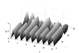
For the figures in this paper, 128 modes on the domain were used in the pseudo-spectral approximation; higher mode runs were tested and gave identical results to those using 128 modes. In each figure, a perturbation of the form
was added to the initial condition . The function is a randomly generated, periodic function, normalized so that , while is typically . However, in certain cases consider , and where this is the case, it is noted. Finally, given the identities derived for the convolution in this paper, the convolution integral turns into a simple term by term multiplication of two vectors in the pseudo-spectral method. Thus no approximations to the integral or kernel are made. As in decon , we convolve against . In every figure, and are one.
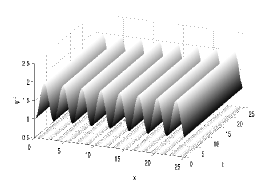
Figure 1a shows the results for , , with nonlocality parameter . As expected from Theorem 4, we see an instability emerge with these parameter values with the random perturbation to the initial condition as explained previously. In contrast, Figure 1b shows the case , , with nonlocality parameter , . The numerics behave as the Theorems 2 and 3 predict. We have confidence that the numerical results are accurate and correspond to the existing theory.
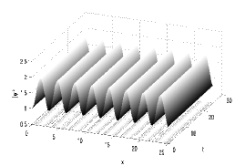
Figures 2a and 2b show the results for the case , , , and . This is a direct comparison to the work in decon . As can be seen from the figures, the underlying solution appears to be robust to perturbations, even with a nonzero nonlocality parameter. This contradicts the results of decon , and seems to imply that (3) is stable in this parameter regime.
VII Conclusion
We have shown that for a large class of kernels, , used to represent long range nonlocal interactions in a Gross-Pitaevskii equation, if one lets the range of nonlocality go to zero, i.e. , then in a rigorous sense, the wavefunction for the nonlocal problem approaches the wavefunction for the local problem. This result holds for any smooth periodic trapping potential . Thus we have demonstrated that generalizing a local model to a nonlocal one can be done in a straightforward way, thus expanding the modeling potential of Gross-Pitaevskii equations. Likewise, we have established the stability properties of a particular class of solutions to a nonlocal Gross-Pitaevskii equation. The theory and numerical experiments predict that when the offset size is large these solutions are stable. It is therefore possible that under the right conditions these solutions could be observed as wavefunctions describing a Bose-Einstein condensate.
Acknowledgments
The author would like to thank M. Ablowitz, B. Deconinck, A. Rey, and H. Segur for reading through earlier versions of this manuscript and for their insightful advice and comments. The author would especially like to thank the authors of decon , B. Deconinck and J.N. Kutz, for their encouragement, interest, and endorsement of the results in this work which was expressed through private communications. The author finally would like to thank the reviewer for helping to make this a significantly better paper.

References
- (1) Lieb, E. H. and Seiringer, R., Proof of Bose-Einstein condensation for dilute trapped gases. Phys. Rev. Lett., 88:170409, 2002.
- (2) Deconinck, B. and Kutz, J.N., Singular instability of exact stationary solutions of the non-local Gross-Pitaevskii equation. Physics Letters A, 319:97–103, 2003.
- (3) Olshanii, M., Atomic scattering in the presence of an external confinement and a gas of impenetrable Bosons. Phys. Rev. Lett., 81:938–941, 1998.
- (4) Ginibre, J. and Velo, G., On a class of nonlinear Schrödinger equations with nonlocal interactions. Math. Z, 170:109–136, 1980.
- (5) Hartmann, B. and Zakrzewski, W.J., Soliton solutions of the nonlinear Schrödinger equation with nonlocal Coulomb and Yukawa interactions. Phys. Let. A, 366:540–544, 2007.
- (6) Sinha, S. and Santos, L., Cold dipolar gases in quasi-one-dimensional geometries. Phys. Rev. Lett. 99:140406, 2007.
- (7) Cuevas, J., Malomed, B.A., Kevrekidis, P.G., and Frantzeskakis, D.J. , Solitons in quasi-one-dimensional Bose-Einstein condensates with competeing dipolar and local interactions Phys. Rev. A, 79:053608, 2009.
- (8) Ghofraniha, N., Conti, C., Ruocco, G., and Trillo, S., Shocks in nonlocal media. Phys. Rev. Lett., 99:043903, 2007.
- (9) Cao, Y., Musslimani, Z.H., and Titi, E.S., Modulation theory for self-focusing in the nonlinear Schrödinger–Helmholtz equation. Numer. Funct. Anal. Optim., 30:46–69, 2009
- (10) Cao, Y., Musslimani, Z.H., and Titi, E.S., Nonlinear Schrödinger–Helmholtz equation as numerical regularization of the nonlinear Schrödinger equation. Nonlinearity, 21:879–898, 2008
- (11) Grillakis, M., Shatah, J., and Strauss, W., Stability theory of solitary waves in the presence of symmetry, I. J. Funct. Anal., 74:160–197, 1987.
- (12) Folland, G., Real Analysis: Modern Techniques and Their Applications. Wiley, New York, NY, 1999.
- (13) Engel, K.J., and Nagel, R., One-Parameter Semigroups and Linear Evolution Equations. Springer, New York, NY, 2000.
- (14) Tao, T., Nonlinear Dispersive Equations: Local and Global Analysis. AMS, Providence, R.I., 2006.
- (15) Linares, F. and Ponce, G., Introduction to Nonlinear Dispersive Equations. New York, NY, 2009.
- (16) Lax, P.D., Functional Analysis. Wiley-Interscience, New York, NY, 2002.
- (17) Chow, S. and Hale, J., Methods of Bifurcation Theory. Springer-Verlag, New York, NY, 1982.
- (18) Kapitula, T., Kevrekidis, P.G., and Sandstede, B., Counting eigenvalues via the Krein signature in infinite-dimensional Hamiltonian systems. Physica D, 195:263–282, 2004.
- (19) Hǎrǎguş, M. and Kapitula, T., On the spectra of periodic waves for infinite-dimensional Hamiltonian systems. Physica D, 237:2649–2671, 2008.
- (20) Magnus, W. and Winkler, S., Hill’s Equation. Interscience, New York, NY, 1966.
- (21) Kato, T., Perturbation Theory for Linear Operators. Springer-Verlag, Berlin, 1995.
- (22) Ben-Yu, G., Spectral Methods and Their Applications. World Scientific, River Edge, NJ, 1998.