Accuracy and Stability of The Continuous-Time 3DVAR Filter for The Navier-Stokes Equation

Abstract

The 3DVAR filter is prototypical of methods used to combine observed data with a dynamical system, online, in order to improve estimation of the state of the system. Such methods are used for high dimensional data assimilation problems, such as those arising in weather forecasting. To gain understanding of filters in applications such as these, it is hence of interest to study their behaviour when applied to infinite dimensional dynamical systems. This motivates study of the problem of accuracy and stability of 3DVAR filters for the Navier-Stokes equation.

We work in the limit of high frequency observations and derive continuous time filters. This leads to a stochastic partial differential equation (SPDE) for state estimation, in the form of a damped-driven Navier-Stokes equation, with mean-reversion to the signal, and spatially-correlated time-white noise. Both forward and pullback accuracy and stability results are proved for this SPDE, showing in particular that when enough low Fourier modes are observed, and when the model uncertainty is larger than the data uncertainty in these modes (variance inflation), then the filter can lock on to a small neighbourhood of the true signal, recovering from order one initial error, if the error in the observations modes is small. Numerical examples are given to illustrate the theory.

1 Introduction

Data assimilation is the problem of estimating the state variables of a dynamical system, given observations of the output variables. It is a challenging and fundamental problem area, of importance in a wide range of applications. A natural framework for approaching such problems is that of Bayesian statistics, since it is often the case that the underlying model and/or the data are uncertain. However, in many real world applications, the dimensionality of the underlying model and the vast amount of available data makes the investigation of the Bayesian posterior distribution of the model state given data computationally infeasible in on-line situations. An example of such an application is the global weather prediction: the computational models used currently involve on the order of $\mathcal{O}(10^{8})$ unknowns, while a large amount of partial observations of the atmosphere, currently on the order of $\mathcal{O}(10^{6})$ per day, are used to compensate both the uncertainty in the model and in the initial conditions.

In situations like this practitioners typically employ some form of approximation based on both physical insight and computational expediency. There are two competing methodologies for data assimilation which are widely implemented in practice, the first being filters [23] and the second being variational methods [3]. In this paper we focus on the filtering approach. Many of the filtering algorithms implemented in practice are ad hoc and, besides some very special cases, the theoretical understanding of their ability to accurately and reliably estimate the state variables is under-developed. Our goal here is to contribute towards such theoretical understanding. We concentrate on the 3DVAR filter which has its origin in weather forecasting [25] and is prototypical of more sophisticated filters used today.

The idea behind filtering is to update the posterior distribution of the system state sequentially at each observation time. This may be performed exactly for linear systems subject to Gaussian noise: the Kalman filter [21]. For the case of non-linear and non-Gaussian scenarios the particle filter [13] can be used and provably approximates the desired probability distribution as the number of particles increases [2]. Nevertheless, standard implementations of this method perform poorly in high dimensional systems [31]. Thus the development of practical filtering algorithms for high dimensional dynamical systems is an active research area and for further insight into this subject the reader may consult [36, 15, 38, 20, 26, 7, 39, 4] and references within. Many of the methods used invoke some form of ad hoc Gaussian approximation and the 3DVAR method which we analyze here is perhaps the simplest example of this idea. These ad hoc filters, 3DVAR included, may also be viewed within the framework of nonlinear control theory and thereby derived directly, without reference to the Bayesian probabilistic interpretation; indeed this is primarily how the algorithms were conceived.

In this paper we will study accuracy and stability for the 3DVAR filter. The term accuracy refers to establishing closeness of the filter to the true signal underlying the data, and stability is concerned with studying the distance between two filters, initialized differently, but driven by the same noisy data. Proving filter accuracy and stability results for control systems has a long history and the paper [32] is a fundamental contribution to the subject with results closely related to those developed here. However, as indicated above, the high dimensionality of the problems arising in data assimilation is a significant challenge in the area. In order to confront this challenge we work in an infinite dimensional setting, therby ensuring that our results are not sensitive to dimensionality. We focus on dissipative dynamical systems, and take the two dimensonal Navier-Stokes equation as a prototype model in this area. Furthermore, we study a data assimilation setting in which data arrives continuously in time which is a natural setting in which to study high time-frequency data subject to significant uncertainty. The study of accuracy and stability of filters for data assimilation has been a developing area over the last few years and the paper [6] contains finite dimensional theory and numerical experiments in a variety of finite and discretized infinite dimensional systems extend the conclusions of the theory. The paper [37] highlights the principle that, roughly speaking, unstable directions must be observed and assimilated into the estimate and, more subtly, that accuracy can be improved by avoiding assimilation of stable directions. In particular the papers [6, 37] both explicitly identify the importance of observing the unstable components of the dynamics, leading to the notion of AUS: assimilation in the unstable subspace. The paper [5] describes a theoretical analysis of 3DVAR applied to the Navier-Stokes equation, when the data arrives in discrete time, and in this paper we address similar questions in the continuous time setting; both papers include the possibility of only partial observations in Fourier space. Taken together, the current paper and [5] provide a significant generalization of the theory in [32] to dissipative infinite dimensional dynamical systems prototypical of the high dimensional problems to which filters are applied in practice; furthermore, through studying partial observations, they give theoretical insight into the idea of AUS as developed in [6, 37]. The infinite dimensional nature of the problem brings fundamental mathematical issues into the problem, not addressed in previous finite dimensional work. We make use of the squeezing property of many dissipative dynamical systems [8, 34], including the Navier-Stokes equation, which drives many theoretical results in this area, such as the ergodicity studies pioneered by Mattingly [27, 19]. In particular our infinite dimensional analysis is motivated by the theory developed in [28] and [22], which are the first papers to study data assimilation directly through PDE analysis, using ideas from the theory of determining modes in infinite dimensional dynamical systems. However, in contrast to those papers, here we allow for noisy observations, and provide a methodology that opens up the possibility of studying more general Gaussian approximate filters such as the Ensemble and the Extended Kalman filter (EnKF and ExKF).

Our point of departure for analysis is an ordinary differential equation (ODE) in a Banach space. Working in the limit of high frequency observations we formally derive continuous time filters. This leads to a stochastic differential equation for state estimation, combining the original dynamics with extra terms indcuing mean reversion to the noisily observed signal. In the particular case of the Navier-Stokes equation we get a stochastic PDE (SPDE) with additional mean-reversion term, driven by spatially-correlated time-white noise. This SPDE is central to our analysis as it is used to prove accuracy and stability results for the 3DVAR filter. In particular, in the case when enough of the low modes of the Navier-Stokes equation are observed and the model has larger uncertainty than the data in these low modes, a situation known to practitioners as variance inflation, then the filter can lock on to a small neighbourhood of the true signal, recovering from the initial error, if the error in the observed modes is small. The results are formulated in terms of the theory of random and stochastic dynamical systems [1], and both forward and pullback type results are proved, leading to a variety of probabilistic accuracy and stability results, in the mean square, probability and almost sure senses.

The paper is organised as follows. In Section 2 we derive the continuous-time limit of the 3DVAR filter applied to a general ODE in a Banach space, by considering the limit of high frequency observations. In Section 3, we focus on the 2D Navier-Stokes equations and present the continuous time 3DVAR filter within this setting. Sections 4 and 5 are devoted, respectively, to results concerning forward accuracy and stability as well as pullback accuracy and stability, for the filter when applied to the Navier-Stokes equation. In Section 6, we present various numerical investigations that corroborate our theoretical results. Finally in Section 7 we present conclusions.

2 Continuous-Time Limit of 3DVAR

Consider $u$ satisfying the following ODE in a Banach space $X:$

$$\frac{du}{dt}=\mathcal{F}(u),\quad u(0)=u_{0}\;.$$ (1)

Our aim is to study online filters which combine knowledge of this dynamical system with noisy observations of $u_{n}=u(nh)$ to estimate the state of the system. This is particularly important in applications where $u_{0}$ is not known exactly, and the noisy data can be used to compensate for this lack of initial knowledge of the system state.

In this section we study approximate Gaussian filters in the high frequency limit, leading to stochastic differential equations which combine the dynamical system with data to estimate the state. As the formal derivation of continuous time filters in this section is independent of the precise model under consideration, we employ the general framework of (1). We make some general observations, relating to a broad family of approximate Gaussian filters, but focus mainly on 3DVAR. In subsequent sections, where we study stability and accuracy of the filter, we focus exclusively on 3DVAR, and work in the context of the $2$D incompressible Navier-Stokes equation, as this is prototypical of dissipative semilinear partial differential equations.

2.1 Set Up - The Filtering Problem

We assume that $u_{0}\sim N(\widehat{m}_{0},\widehat{C}_{0})$ so that the initial data is only known statistically. The objective is to update the estimate of the state of the system sequentially in time, based on data received sequentially in time. We define the flow-map $\Psi:X\times\mathbb{R}^{+}\to X$ so that the solution to (1) is $u(t)=\Psi(u_{0};t)$. Let $H$ denote a linear operator from $X$ into another Banach space $Y$, and assume that we observe $Hu$ at equally spaced time intervals:

$$y_{n}=H\Psi(u_{0};nh)+\eta_{n}.$$ (2)

Here $\{\eta_{n}\}_{n\in\mathbb{N}}$ is an i.i.d sequence, independent of $u_{0}$, with $\eta_{1}\sim N(0,\Gamma).$ If we write $u_{n}=\Psi(u_{0};nh)$, then

$$u_{n+1}=\Psi(u_{n};h),$$ (3)

and

$$y_{n}|u_{n}\sim N\bigl{(}Hu_{n},\Gamma).$$ (4)

We denote the accumulated data up to the time $n$ by

$$Y_{n}=\{y_{i}\}^{n}_{i=1}.$$

Our aim is to find $\mathbb{P}(u_{n}|Y_{n}).$

We will make the Gaussian ansatz that

$$\mathbb{P}(u_{n}|Y_{n})\simeq N(\widehat{m}_{n},\widehat{C}_{n}).$$ (5)

The key question in designing an approximate Gaussian filter, then, is to find an update rule of the form

$$(\widehat{m}_{n},\widehat{C}_{n})\mapsto(\widehat{m}_{n+1},\widehat{C}_{n+1})$$ (6)

Because of the linear form of the observations in (2), together with the fact that the noise is mean zero-Gaussian, this update rule is determined directly if we impose a further Gaussian ansatz, now on the distribution of $u_{n+1}$ given $Y_{n}:$

$$u_{n+1}|Y_{n}\sim N(m_{n+1},C_{n+1})$$ (7)

With this in mind, the update (6) is usually split into two parts. The first, prediction (or forecast), step is the map

$$(\widehat{m}_{n},\widehat{C}_{n})\mapsto(m_{n+1},C_{n+1})$$ (8)

The second, analysis, step is

$$(m_{n+1},C_{n+1})\mapsto(\widehat{m}_{n+1},\widehat{C}_{n+1}).$$ (9)

For the prediction step we will simply impose the approximation (7) with

$$m_{n+1}=\Psi(\widehat{m}_{n};h),$$ (10)

while the choice of $C_{n+1}$ will depend on the choice of the specific filter. For the analysis step, assumptions (4), (7) imply that

$$u_{n+1}|Y_{n+1}\sim N(\widehat{m}_{n+1},\widehat{C}_{n+1})$$ (11)

and an application of Bayes rule, as applied in the standard Kalman filter update [21], and using (10), gives us the nonlinear map (6) in the form

$$\widehat{C}_{n+1} = C_{n+1}-C_{n+1}H^{*}(\Gamma+HC_{n+1}H^{*})^{-1}HC_{n+1}$$ (12a)

$$\widehat{m}_{n+1} = \Psi(\widehat{m}_{n};h)+C_{n+1}H^{*}(\Gamma+HC_{n+1}H^{*})^{-1}(y_{n+1}-Hm_{n+1})$$ (12b)

The mean $\widehat{m}_{n+1}$ is an element of the Banach space $X$, and $\widehat{C}_{n+1}$ is a linear symmetric and non-negative operator from $X$ into itself.

2.2 Derivation of The Continuous-Time Limit

Together equations (10) and (12), which are generic for any approximate Gaussian filter, specify the update for the mean once the equation determining $C_{n+1}$ is defined. We proceed to derive a continuous-time limit for the mean, in this general setting, assuming that $C_{n}$ arises as an approximation of a continuous process $C(t)$ evaluated at $t=nh$, so that $C_{n}\approx C(nh)$, and that $h\ll 1$. Throughout we will assume that $\Gamma=h^{-1}\Gamma_{0}$. This scaling implies that the noise variance is inversely proportional to the time between observations and is the relationship which gives a nontrivial stochastic limit as $h\to 0.$

With these scaling assumptions equation (12b) becomes

$$\widehat{m}_{n+1}=\Psi(\widehat{m}_{n};h)+hC_{n+1}H^{*}(\Gamma_{0}+hHC_{n+1}H^{*})^{-1}\bigl{(}y_{n+1}-H\Psi(\widehat{m}_{n};h)\bigr{)}.$$

Thus

$$\frac{\widehat{m}_{n+1}-\widehat{m}_{n}}{h}=\frac{\Psi(\widehat{m}_{n};h)-\widehat{m}_{n}}{h}+C_{n+1}H^{*}(\Gamma_{0}+hHC_{n+1}H^{*})^{-1}\bigl{(}y_{n+1}-H\Psi(\widehat{m}_{n};h)\bigr{)}.$$

If we define the sequence $\{z_{n}\}_{n\in\mathbb{Z}^{+}}$ by

$$z_{n+1}=z_{n}+hy_{n+1},\quad z_{0}=0\;,$$

then we can rewrite the previous equation as

$$\frac{\widehat{m}_{n+1}-\widehat{m}_{n}}{h}= \frac{\Psi(\widehat{m}_{n};h)-\widehat{m}_{n}}{h}$$ (13)

$$\quad\quad\quad+C_{n+1}H^{*}(\Gamma_{0}+hHC_{n+1}H^{*})^{-1}\left(\frac{z_{n+1}-z_{n}}{h}-H\Psi(\widehat{m}_{n};h)\right).$$

Note that

$$\Psi(\widehat{m}_{n};h)=\widehat{m}_{n}+h\mathcal{F}(\widehat{m}_{n})+\mathcal{O}(h^{2}).$$

This is an Euler-Maruyama-like discretization of a stochastic differential equation which, if we pass to the limit of $h\rightarrow 0$ in (13), noting that we have assumed that $C_{n}\approx C(nh)$ for some continuous covariance process, is seen to be

$$\frac{d\widehat{m}}{dt}=\mathcal{F}(\widehat{m})+CH^{*}\Gamma^{-1}_{0}\left(\frac{dz}{dt}-H\widehat{m}\right),\quad\widehat{m}(0)=\widehat{m}_{0}.$$ (14)

Equation (14) is similar to the observer equation in the nonlinear control literature [32]. Our objective in this paper is to study the stability and accuracy properties of this stochastic model. Here stability refers to the contraction of two different trajectories of the filter (14), started at two different points, but driven by the same observed data; and accuracy refers to estimating the difference between the true trajectory of (1) which underlies the data, and the output of the filter (14). Similar questions are studied in finite dimensions in [32]. However, the infinite dimensional nature of our problem, coupled with the fact that we study situations where the state is only partially observed ($H$ is not invertible on $X$) mean that new techniques of analysis are required, building on the theory of semilinear dissipative PDEs and infinite dimensional dynamical systems.

We now express the observation signal $z$ in terms of the truth $u$ in order to facilitate study of filter stability and accuracy. In particular, we have that

$$\left(\frac{z_{n+1}-z_{n}}{h}\right)=y_{n+1}=Hu_{n+1}+\frac{\sqrt{\Gamma_{0}}}{\sqrt{h}}\Delta w_{n+1},$$

where $\{\Delta w_{n}\}_{n\in\mathbb{N}}$ is an i.i.d sequence and $\Delta w_{1}\sim N(0,I)$ in $Y$. This corresponds to the Euler-Maruyama discretization of the SDE

$$\frac{dz}{dt}=Hu+\sqrt{\Gamma_{0}}\frac{dW}{dt},\quad z(0)=0.$$ (15)

Expressed in terms of the true signal $u$, equation (14) becomes

$$\frac{d\widehat{m}}{dt}=\mathcal{F}(\widehat{m})+CH^{*}\Gamma^{-1}_{0}H\left(u-\widehat{m}\right)+{\color[rgb]{1,0,1}C}H^{*}\Gamma^{-1/2}_{0}\frac{dW}{dt}.$$ (16)

We complete the study of the continuous limit with the specific example of 3DVAR. This is the simplest filter of all in which the prediction step is found by simply setting $C_{n+1}=\widehat{C}$ for some fixed covariance operator $\widehat{C}$, independent of $n$. Then equation (12) shows that ${\widehat{C}}_{n+1}=\widehat{C}+{\cal O}(h)$ and we deduce that the limiting covariance is simply constant: $C(t)=\widehat{C}(t)=\widehat{C}$ for all $t\geq 0$. The present work will focus on this case and hence study (16) in the case where $C=\widehat{C}$, a constant in time.

3 Continuous-Time 3DVAR for Navier-Stokes

In this section we describe application of the 3DVAR algorithm to the two dimensional Navier-Stokes equation. This will form the focus of the remainder of the paper. In subsection 3.1 we describe the forward model itself, namely we specify equation (1), and then in subsection 3.2 we describe how data is incorporated into the model, and specify equation (16), and the choices of the (constant in time) operators $C=\widehat{C}$ and $\Gamma_{0}$ which appear in it.

3.1 Forward Model

Let $\mathbb{T}^{2}$ denote the two-dimensional torus of side $L:$ $[0,L)\times[0,L)$ with periodic boundary conditions. We consider the equations

$$\begin{array}[]{ccc}\partial_{t}u(x,t)-\nu\Delta u(x,t)+u(x,t)\cdot\nabla u(x,t)+\nabla p(x,t)&=&f(x)\\ \nabla\cdot u(x,t)&=&0\\ u(x,0)&=&u_{0}(x)\end{array}$$

for all $x\in\mathbb{T}^{2}$ and $t\in(0,\infty)$. Here $u\colon\mathbb{T}^{2}\times(0,\infty)\to\mathbb{R}^{2}$ is a time-dependent vector field representing the velocity, $p\colon\mathbb{T}^{2}\times(0,\infty)\to\mathbb{R}$ is a time-dependent scalar field representing the pressure and $f\colon\mathbb{T}^{2}\to\mathbb{R}^{2}$ is a vector field representing the forcing which we take as time-independent for simplicity. The parameter $\nu$ represents the viscosity. We assume throughout that $u_{0}$ and $f$ have average zero over $\mathbb{T}^{2}$; it then follows that $u(\cdot,t)$ has average zero over $\mathbb{T}^{2}$ for all $t>0$.

Define

$${\mathsf{T}}:=\left\{{\rm{trigonometric\,polynomials\,}}u:\mathbb{T}^{2}\to{\mathbb{R}}^{2}\,\Bigl{|}\,\nabla\cdot u=0,\,\int_{\mathbb{T}^{2}}u(x)\,\mathrm{d}x=0\right\}$$

and $\mathcal{H}$ as the closure of ${\mathsf{T}}$ with respect to the norm in $(L^{2}(\mathbb{T}^{2}))^{2}=L^{2}(\mathbb{T}^{2},\mathbb{R}^{2})$.

We let $P:(L^{2}(\mathbb{T}^{2}))^{2}\to\mathcal{H}$ denote the Leray-Helmholtz orthogonal projector. Given $k=(k_{1},k_{2})^{\mathrm{T}}$, define $k^{\perp}:=(k_{2},-k_{1})^{\mathrm{T}}$. Then an orthonormal basis for $\mathcal{H}$ is given by $\psi_{k}\colon\mathbb{R}^{2}\to\mathbb{R}^{2}$, where

$$\psi_{k}(x):=\frac{k^{\perp}}{|k|}\exp\Bigl{(}\frac{2\pi ik\cdot x}{L}\Bigr{)}$$ (17)

for $k\in\mathbb{Z}^{2}\setminus\{0\}$. Thus for $u\in\mathcal{H}$ we may write

$$u(x,t)=\sum_{k\in\mathbb{Z}^{2}\setminus\{0\}}u_{k}(t)\psi_{k}(x)$$

where, since $u$ is a real-valued function, we have the reality constraint $u_{-k}=-\overline{u_{k}}.$ We define the projection operators $P_{\lambda}:\mathcal{H}\to\mathcal{H}$ and $Q_{\lambda}:\mathcal{H}\to\mathcal{H}$ for $\lambda\in\mathbb{N}\cup\{\infty\}$ by

$$P_{\lambda}u(x,t)=\sum_{|2\pi k|^{2}<\lambda L^{2}}u_{k}(t)\psi_{k}(x),\quad Q_{\lambda}=I-P_{\lambda}.$$

Below we will choose the observation operator $H$ to be $P_{\lambda}.$

We define $A=-\frac{L^{2}}{4\pi^{2}}P\Delta$, the Stokes operator, and, for every $s\in\mathbb{R}$, define the Hilbert spaces $\mathcal{H}^{s}$ to be the domain of $A^{s/2}.$ We note that $A$ is diagonalized in $\mathcal{H}$ in the basis comprised of the $\{\psi_{k}\}_{k\in{\mathbb{Z}}^{2}\backslash\{0\}}$ and that, with the normalization employed here, the smallest eigenvalue of $A$ is $\lambda_{1}=1.$ We use the norm $\|\cdot\|_{s}^{2}:=\langle\cdot,A^{s}\cdot\rangle$, the abbreviated notation $\|u\|$ for the norm on $\mathcal{V}:=\mathcal{H}^{1}$, and $|\cdot|$ for the norm on $\mathcal{H}:=\mathcal{H}^{0}$.

Applying the projection $P$ to the Navier-Stokes equation we may write it as an ODE in $\mathcal{H}$:

$$\frac{\mathrm{d}u}{\mathrm{d}t}+\delta Au+\mathcal{B}(u,u)=f,\quad u(0)=u_{0}.$$ (18)

Here $\delta=4\pi^{2}\nu/L^{2}$ and the term $\mathcal{B}(u,v)$ is the symmetric bilinear form defined by

$$\mathcal{B}(u,v)=\frac{1}{2}P(u\cdot\nabla v)+\frac{1}{2}P(v\cdot\nabla u)$$

for all $u,v\in\mathcal{V}$. Finally, with abuse of notation, $f$ is the original forcing, projected into $\mathcal{H}$. Equation (18) is in the form of equation (1) with

$$\mathcal{F}(u)=-\delta Au-\mathcal{B}(u,u)+f.$$ (19)

See [8] for details of this formulation of the Navier-Stokes equation as an ODE in $\mathcal{H}$. The following proposition is a classical result which implies the existence of a dissipative semigroup for the ODE (18). See Theorems 9.5 and 12.5 in [29] for a concise overview and [33, 34] for further details.

Proposition 3.1.

Assume that $u_{0}\in\mathcal{H}^{1}$ and $f\in\mathcal{H}$. Then (18) has a unique strong solution on $t\in[0,T]$ for any $T>0:$

$$u\in L^{\infty}\bigl{(}(0,T);\mathcal{H}^{1}\bigr{)}\cap L^{2}\bigl{(}(0,T);\mathcal{H}^{2}\bigr{)},\quad\frac{du}{dt}\in L^{2}\bigl{(}(0,T);\mathcal{H}\bigr{)}.$$

Furthermore the equation has a global attractor $\mathcal{A}$ and there is $R\in(0,\infty)$ such that, if $u_{0}\in\mathcal{A}$, then the solution from this initial condition exists for all $t\in\mathbb{R}$ and $\sup_{t\in\mathbb{R}}\|u(t)\|^{2}=R.$

We let $\{\Psi(\cdot,t):\mathcal{H}^{1}\to\mathcal{H}^{1}\}_{t\geq 0}$ denote the semigroup of solution operators for the equation (18) through $t$ time units. We note that by working with weak solutions, $\Psi(\cdot,t)$ can be extended to act on larger spaces $\mathcal{H}^{s}$, with $s\in[0,1)$, under the same assumption on $f$; see Theorem 9.4 in [29].

3.2 3DVAR

We apply the analysis of the previous section to write down the continuous time 3DVAR filter, namely (16) with $C(t)={\widehat{C}}$ constant in time, for the Navier-Stokes equation. We take $X=\mathcal{H}$ and throughout we assume that the data is found by observing $P_{\lambda}u$ at discrete times, so that $H^{*}=H=P_{\lambda}$ and $Y=P_{\lambda}\mathcal{H}$. We assume that $A$, $\Gamma_{0}$ and $\widehat{C}$ commute and, for simplicity of presentation, suppose that

$$\widehat{C}=\omega\sigma_{0}^{2}A^{-2\zeta},\quad\Gamma_{0}=\sigma_{0}^{2}A^{-2\beta}P_{\lambda}.$$ (20)

We set $\alpha=\zeta-\beta$. These assumptions correspond to those made in [5] where discrete time filters are studied. Note that $A^{s/2}$ is defined on $\mathcal{H}^{s}$; it is also defined on $Y$ for every $s\in\mathbb{R}$, provided that $\lambda$ is finite.

From equations (16), using (19) and the choices for $\widehat{C}$ and $\Gamma_{0}$ we obtain

$$\frac{\mathrm{d}\widehat{m}}{\mathrm{d}t}+\delta A\widehat{m}+\mathcal{B}(\widehat{m},\widehat{m})+\omega A^{-2\alpha}P_{\lambda}(\widehat{m}-u)=f+\omega\sigma_{0}A^{-2\alpha-\beta}P_{\lambda}\frac{\mathrm{d}W}{\mathrm{d}t},\quad\widehat{m}(0)=\widehat{m}_{0}$$ (21)

where $W$ is a cylindrical Brownian motion in $Y$. In the following we consider the cases of finite $\lambda$, where the data is in a finite dimensional subspace of $\mathcal{H}$, and infinite $\lambda$, where $P_{\lambda}=I$ and the whole solution is observed.

Lemma 3.2.

For $\lambda=\infty$ assume that $4\alpha+2\beta>1.$ Then the stochastic convolution

$$W_{A}(t)=\int_{0}^{t}e^{\delta(t-s)A}A^{-2\alpha-\beta}P_{\lambda}dW(s)$$

has a continuous version in $C^{0}([0,T],\mathcal{V})$ with all moments $\mathbb{E}\sup_{[0,T]}\|W_{A}\|^{p}$ finite for all $T>0$ and $p>1$.

Proof.

If $\lambda<\infty$ then the covariance of the driving noise is automatically trace-class as it is finite dimensional; since $4\alpha+2\beta>1$ it follows that the covariance of the driving noise is also trace-class when $\lambda=\infty.$ The desired result follows from Theorem 5.16 in [12]. For the moments see [12, (5.23)]. ∎

It is only in the case of full observations (i.e., $\lambda=\infty$) that we need the additional regularity condition $4\alpha+2\beta>1$. This may be rewritten as $\zeta>\frac{1}{4}+\frac{1}{2}\beta$ and relates the rate of decay, in Fourier space, of the model variance to the observational variance. Although a key driver for our accuracy and stability results (see Remark 4.4 below) will be variance inflation, meaning that the observational variance is smaller than the model variance in the low Fourier modes, this condition on $\zeta$ allows regimes in which, for high Fourier modes, the situation is reversed.

Proposition 3.3.

Assume that $u_{0}\in\mathcal{A}$ and let $u$ be the corresponding solution of (18) on the global attractor $\mathcal{A}$. For $\lambda=\infty$ suppose $4\alpha+2\beta>1$ and $\alpha>-\frac{1}{2}.$ Then for any initial condition $\widehat{m}(0)\in\mathcal{H}$ there is a stochastic process $\widehat{m}$ which is the unique strong solution of (21) in the spaces

$$\widehat{m}\in L^{2}\bigl{(}(0,T),\mathcal{V}\bigr{)}\cap C^{0}\bigl{(}[0,T],\mathcal{H}\bigr{)}$$

for all $T>0$. Moreover,

$$\mathbb{E}\|\widehat{m}\|^{2}_{L^{\infty}\bigl{(}(0,T),\mathcal{H}\bigr{)}}+\mathbb{E}\|\widehat{m}\|^{2}_{L^{2}\bigl{(}(0,T),\mathcal{V}\bigr{)}}<\infty.$$

To be more precise

$$\widehat{m}\in L^{2}\Bigl{(}\Omega,C^{0}_{\mathrm{loc}}\bigl{(}[0,\infty),\mathcal{H}\bigr{)}\Bigr{)}\cap L^{2}\Bigl{(}\Omega,L^{2}_{\mathrm{loc}}\bigl{(}[0,\infty),\mathcal{V}\bigr{)}\Bigr{)}\;.$$

Proof.

The proof of this theorem is well known without the function $u$ and the additional linear term. See for example Theorem 15.3.1 in the book [11] using fixed point arguments based on the mild solution. Another reference is [16, Theorem 3.1] based on spectral Galerkin methods. See also [18] or [30]. Nevertheless, our theorem is a straightforward modification of their arguments. For simplicity of presentation we refrain from giving a detailed argument here.

The existence and uniqueness is established either by Galerkin methods or fixed-point arguments. The continuity of solutions follows from the standard fixed-point arguments for the mild formulation in the space $C^{0}\bigl{(}[0,T],\mathcal{H}\bigr{)}$.

Finally, as we assume the covariance of the Wiener process to be trace-class, the bounds on the moments are a straightforward application of Itô’s formula (cf. [12, Theorem 4.17]) to $|\widehat{m}|^{2}$ and to $\|\widehat{m}\|^{2}$, in order to derive standard a-priori estimates. This is very similar to the method of proof that we use to study mean square stability in Section 4.1.

The additional linear term $\omega A^{-2\alpha}P_{\lambda}\widehat{m}$ does not change the result in any substantive fashion. If $\lambda<\infty$ then the proof is essentially identical, as the additional term is a lower order perturbation of the Stokes operator.

If $\lambda=\infty$ then minor modifications of the proof are necessary, but do not change the proof significantly. This is since, for $\alpha>-\frac{1}{2}$, the additional term $\omega A^{-2\alpha}\widehat{m}$ is a compact perturbation of the Stokes operator.

The additional forcing term, depending on $u$, is always sufficiently regular for our argument, as we assume $u$ to be on the attractor (see Proposition 3.1). ∎

Remark 3.4.

For $\lambda=\infty$ it is possible to extend the preceding result to other ranges of $\alpha$, but this will change the proof. Hence, for simplicity, for $\lambda=\infty$ we always assume that $\alpha>-\frac{1}{2}$.

We comment later on the fact that the solutions to (21) generate a stochastic dynamical system. As we need two-sided Wiener-processes for this we postpone the discussion to Section 5.

4 Forward Accuracy and Stability

We wish to study conditions under which two filters, starting from different points but driven by the same observations, converge (stability); and conditions under which the filter will, asymptotically, track the true signal (accuracy). Establishing such results has been the object of study in control theory for some time, and the paper [32] contains foundational work in both the discrete and continuous time settings. However the infinite dimensional nature of the problem at hand brings significant new challenges to the analysis. The key idea driving the proofs is that, although the Navier-Stokes equations themselves may admit exponentially diverging trajectories, the observations can counteract this instability, provided the observation space is large enough. Roughly speaking the exponential divergence of the Navier-Stokes equations is dominated by a finite set low Fourier modes, whilst the rest of the space contracts. If the observations provide information about enough of the low Fourier modes, then this can counteract the instability. This basic idea underlies the accuracy and stability results proved in subsections 4.1 and 4.2.

A key technical estimate in what follows is the following (see [35]):

Lemma 4.1.

For the symmetric bilinear map

$$\mathcal{B}(u,v)=\tfrac{1}{2}P(u\cdot\nabla v)+\tfrac{1}{2}P(v\cdot\nabla u)$$

there is constant $K^{\prime}\geq 1$ such that for all $v,w\in\mathcal{V}$

$$\langle\mathcal{B}(v,v)-\mathcal{B}(w,w),v-w\rangle\leq K^{\prime}\|w\|\|v-w\|\cdot|v-w|,$$ (22)

$$|\langle\mathcal{B}(w,v),v\rangle|\leq K^{\prime}\|w\|\|v\||v|\quad\text{and}\quad|\langle\mathcal{B}(w,v),z\rangle|\leq K^{\prime}\|v\|\|w\|\|z\|\;.$$ (23)

Furthermore, for all $v\in\mathcal{V}$,

$$\langle\mathcal{B}(v,v),v\rangle=0$$ (24)

Notice that (22) implies that, for $K=(K^{\prime})^{2}/\delta$,

$$\langle\mathcal{B}(v,v)-\mathcal{B}(w,w),v-w\rangle\leq\tfrac{1}{2}K\|w\|^{2}|v-w|^{2}+\tfrac{1}{2}\delta\|v-w\|^{2},\quad\forall v,w\in\mathcal{V}.$$ (25)

This estimate will be used to control the possible exponential divergence of Navier-Stokes trajectories which needs to be compensated for by means of observations.

Proof of Lemma 4.1..

We give a brief overview of the main ideas required to prove this well known result. First notice that the assumption $K^{\prime}\geq 1$ is without loss of generality. We need this later for simplicity of presentation.

Then (22) is a direct consequence of (23) and (24), by using the identity

$$\mathcal{B}(v,v)-\mathcal{B}(w,w)=\mathcal{B}(v+w,v-w)=\mathcal{B}(v-w,v-w)+2\mathcal{B}(w,v-w)$$

For simplicity of presentation, we use the same constant in (22) and (23).

For Navier-Stokes it is well-known that $\langle(w\cdot\nabla)v,v\rangle=0$, as the divergence of $w$ is $0$. Thus there is constant $c_{1}$ such that

$$2|\langle\mathcal{B}(w,v),v\rangle|=\langle(v\cdot\nabla)w,v\rangle|\leq c_{1}\|w\||v|_{L^{4}}^{2}\;.$$

Since, in two dimensions $H^{1/2}=D(A^{1/4})$ is embedded into $L^{4}$, there is constant $c_{2}$ such that $|\langle\mathcal{B}(w,v),z\rangle|\leq c_{2}\|w\|\|v\|_{H^{\frac{1}{2}}}\|z\|_{H^{\frac{1}{2}}}\;.$ The first result in (23) then follows from the interpolation inequality $\|v\|^{2}_{H^{\frac{1}{2}}}\leq c|v|\|v\|$ and the second from the embedding $\|v\|_{H^{\frac{1}{2}}}\leq c\|v\|$. ∎

Finally, in the following a key role will be played by the constant $\gamma$ defined as follows:

Assumption 4.2.

Let $\gamma$ be the largest positive constant such that

$$\frac{1}{2}\gamma|h|^{2}\leq\langle\omega A^{-2\alpha}P_{\lambda}h,h\rangle+\frac{1}{2}\delta\|h\|^{2}\qquad\text{for all }h\in\mathcal{V}.$$ (26)

It is clear that such a $\gamma$ always exists, and indeed that $\gamma\geq\delta$, as one has $\langle A^{-2\alpha}P_{\lambda}h,h\rangle\geq 0$. We will study how $\gamma$ depends on $\lambda$ and $\omega$ in subsequent discussions where we show that, by choosing $\lambda$ and $\omega$ large enough, $\gamma$ can be made arbitrarily large.

4.1 Forward Mean Square Accuracy

Theorem 4.3 (Accuracy).

Let $\widehat{m}$ solve (21), and let $u$ solve (18) with initial condition on the global attractor $\mathcal{A}$. For $\lambda=\infty$ assume $4\alpha+2\beta>1$ and $\alpha>-\frac{1}{2}$. Suppose that $\gamma$, the largest positive number such that (26) holds, satisfies

$$\gamma=KR+\gamma_{0}\qquad\text{for some }\gamma_{0}>0,$$

where $K$ is the constant appearing in (25) and $R$, recall, is defined by $R=\sup_{t\in\mathbb{R}}\|u(t)\|^{2}$. Then

$$\mathbb{E}|\widehat{m}(t)-u(t)|^{2}\leq\mathrm{e}^{-\gamma_{0}t}|\widehat{m}(0)-u(0)|^{2}+\omega^{2}\sigma_{0}^{2}\int_{0}^{t}\mathrm{e}^{-\gamma_{0}(t-s)}{{\mathrm{trace}}}_{\mathcal{H}}\bigl{(}A^{-4\alpha-2\beta}P_{\lambda}\bigr{)}ds.$$

As a consequence

$$\limsup_{t\to\infty}\mathbb{E}|\widehat{m}(t)-u(t)|^{2}\leq\tfrac{1}{\gamma_{0}}\omega^{2}\sigma_{0}^{2}{{\mathrm{trace}}}_{\mathcal{H}}\bigl{(}A^{-4\alpha-2\beta}P_{\lambda}\bigr{)}.$$

Proof.

Define the error $e=\widehat{m}-u$ and subtract equation (18) from (21) to obtain

$$de+\delta Ae=\Bigl{(}\mathcal{B}(u,u)-\mathcal{B}(\widehat{m},\widehat{m})-\omega A^{-2\alpha}P_{\lambda}e\Bigr{)}dt+\omega\sigma_{0}A^{-2\alpha-\beta}P_{\lambda}dW\;.$$

Using the Itô formula from Theorem 4.17 of [12], together with (25), yields

$$\tfrac{1}{2}d|e|^{2}\leq \Bigl{(}-\tfrac{1}{2}\delta\|e\|^{2}+\tfrac{1}{2}K\|u(t)\|^{2}|e|^{2}-\langle\omega A^{-2\alpha}P_{\lambda}e,e\rangle\Bigr{)}dt$$

$$\qquad\qquad+\langle e,\omega\sigma_{0}A^{-2\alpha-\beta}P_{\lambda}dW\rangle+\tfrac{1}{2}\omega^{2}\sigma_{0}^{2}{{\mathrm{trace}}}_{\mathcal{H}}\bigl{(}A^{-4\alpha-2\beta}P_{\lambda}\bigr{)}dt\;.$$

Here we have used the fact that the projection $P_{\lambda}$ and $A$ commute. Applying (26) and taking expectations we obtain

$$\frac{d}{dt}\mathbb{E}|e(t)|^{2}\leq-\bigl{(}\gamma-K\|u(t)\|^{2}\bigr{)}\cdot\mathbb{E}|e(t)|^{2}+\omega^{2}\sigma_{0}^{2}{{\mathrm{trace}}}_{\mathcal{H}}\bigl{(}A^{-4\alpha-2\beta}P_{\lambda}\bigr{)}\;,$$

But $\sup_{t\geq 0}\|u(t)\|^{2}=R<\infty$ by Proposition 3.1 and hence, by assumption on $\gamma$,

$$\frac{d}{dt}\mathbb{E}|e(t)|^{2}\leq-\gamma_{0}\cdot\mathbb{E}|e(t)|^{2}+\omega^{2}\sigma_{0}^{2}{{\mathrm{trace}}}_{\mathcal{H}}\bigl{(}A^{-4\alpha-2\beta}P_{\lambda}\bigr{)}.\;,$$

The result follows from a Gronwall argument. ∎

Remark 4.4.

We now briefly discuss the choice of parameters to ensure satisfaction of the conditions of Theorem 4.3, and its implications. To this end, notice that $K$ and $R$ are independent of the parameters of the filter, being determined entirely by the Navier-Stokes equation (18) itself. To apply the theorem we need to ensure that $\gamma$ defined by (26) exceeds $KR.$ Notice that

$$\frac{1}{2}\gamma|h|^{2}\leq\langle\omega A^{-2\alpha}P_{\lambda}h,h\rangle+\frac{1}{2}\delta\|h\|^{2}\qquad\text{for all }h\in P_{\lambda}\mathcal{V}$$

requires that

$$\frac{1}{2}\gamma\leq\frac{\omega}{|k|^{4\alpha}}+\frac{1}{2}\delta|k|^{2}\qquad\text{for all }|k|^{2}<\lambda L^{2}/4\pi^{2}.$$ (27)

On the other hand,

$$\frac{1}{2}\gamma|h|^{2}\leq\langle\omega A^{-2\alpha}P_{\lambda}h,h\rangle+\frac{1}{2}\delta\|h\|^{2}\qquad\text{for all }h\in Q_{\lambda}\mathcal{V}$$

requires that

$$\gamma\leq\delta|k|^{2}\qquad\text{for all }|k|^{2}\geq\lambda L^{2}/4\pi^{2}.$$ (28)

Since the global minimum of the function $x\in\mathbb{R}^{+}\mapsto\omega x^{-2\alpha}+\frac{1}{2}\delta x$ occurs at a point $c\delta^{2\alpha/2\alpha+1}\omega^{1/2\alpha+1}$ we see that the maximum value of $\gamma$ such that (26) holds, $\gamma_{\rm max}$, is

$$\gamma_{\rm max}=\min\Big{\{}\frac{\delta\lambda L^{2}}{4\pi^{2}},c(\delta^{2\alpha}\omega)^{1/(2\alpha+1)}\Big{\}}.$$

This demonstrates that, provided $\lambda$ is large enough, and $\omega$ is large enough, then the conditions of the theorem are satisfied.

In summary, these conditions are satisfied provided that enough of the low Fourier modes are observed ($\lambda$ large enough), and provided that the ratio of the scale of the covariance for the model to that for the observations, $\omega$, is sufficiently large. Ensuring that the latter is achieved is often termed variance inflation in the applied literature and our theory provides concrete analytical insight into the mechanisms behind it. Furthermore, notice that once $\lambda$ and $\omega$ are chosen to ensure this, then the asymptotic mean square error will be small, provided $\epsilon:=\omega\sigma_{0}$ is small that is, provided the observational noise is sufficiently small. In this situation the theorem establishes a form of accuracy of the filter since, regardless of the starting point of the filter,

$$\limsup_{t\to\infty}\mathbb{E}|\widehat{m}(t)-u(t)|^{2}\leq\frac{1}{\gamma_{0}}\epsilon^{2}{{\mathrm{trace}}}_{\mathcal{H}}\bigl{(}A^{-4\alpha-2\beta}P_{\lambda}\bigr{)}.$$

4.2 Forward Stability in Probability

The aim of this section is to prove that two different solutions of the continuous 3DVAR filter will converge to one another in probability as $t\to\infty.$ Almost sure and mean square convergence is out of reach in forward time. However, almost sure pullback convergence is possible and we study this in the next section.

Throughout this section we define, for $u$ on the attractor,

$$R^{\prime}=\sup_{t\in\mathbb{R}}|f+\omega A^{-2\alpha}P_{\lambda}u|_{-1}^{2}$$ (29)

and we assume that $R^{\prime}<\infty.$ From this we define

$$R^{\prime\prime}=\frac{K}{\delta^{2}}R^{\prime}+\frac{K}{\delta}\omega^{2}\sigma_{0}^{2}{{\mathrm{trace}}}_{\mathcal{H}}\bigl{(}A^{-4\alpha-2\beta}P_{\lambda}\bigr{)}.$$ (30)

Theorem 4.5.

Let $\widehat{m}_{i}$ solve (21) with initial condition $\widehat{m}(0)=\widehat{m}_{i}(0)$ and let $u$ solve (18) with initial condition on the global attractor $\mathcal{A}$. For $\lambda=\infty$ assume that $4\alpha+2\beta>1$ and $\alpha>-\frac{1}{2}$. Let $R^{\prime\prime}$ be defined as above, and suppose $\gamma$, the largest positive number such that (26) holds, satisfies $\gamma=R^{\prime\prime}+\gamma_{0}$ for some $\gamma_{0}>0.$

Then for all $\eta\in(0,\gamma_{0})$

$$|\widehat{m}_{1}(t)-\widehat{m}_{2}(t)|e^{\eta t}\to 0\qquad\text{in probability as }t\to\infty.$$

Proof.

It follows from Lemma 4.6 below that, for any fixed $t>0$,

$$\mathbb{P}\Big{(}|\widehat{m}_{1}(t)-\widehat{m}_{2}(t)|^{2}\leq|\widehat{m}_{1}(0)-\widehat{m}_{2}(0)|^{2}e^{-2\gamma_{0}t}\Big{)}\geq\mathbb{P}\Big{(}\frac{1}{t}\int_{0}^{t}K\|\widehat{m}_{2}(s)\|^{2}ds\leq\gamma-\gamma_{0}\Big{)}\;.$$ (31)

Thus to establish the desired convergence in probability, it suffices to establish that the right hand side converges to $1$ as $t\to\infty$.

Taking the inner-product of equation (21) with $\widehat{m}$, applying (24) and using the Itô formula from Theorem 4.17 of [12], we obtain

$$\tfrac{1}{2}d|\widehat{m}|^{2}\leq \Bigl{(}-\delta\|\widehat{m}\|^{2}-\langle\omega A^{-2\alpha}P_{\lambda}\widehat{m},\widehat{m}\rangle+\langle f+\omega A^{-2\alpha}P_{\lambda}u,\widehat{m}\rangle\Bigr{)}dt$$

$$\qquad\qquad+\langle\widehat{m},\omega\sigma_{0}A^{-2\alpha-\beta}P_{\lambda}dW\rangle+\tfrac{1}{2}\omega^{2}\sigma_{0}^{2}{{\mathrm{trace}}}_{\mathcal{H}}\bigl{(}A^{-4\alpha-2\beta}P_{\lambda}\bigr{)}dt$$

$$\leq \Bigl{(}-\frac{1}{2}\delta\|\widehat{m}\|^{2}+\frac{1}{2\delta}|f+\omega A^{-2\alpha}P_{\lambda}u|^{2}_{-1}\Bigr{)}dt$$

$$\qquad\qquad+\langle\widehat{m},\omega\sigma_{0}A^{-2\alpha-\beta}P_{\lambda}dW\rangle+\tfrac{1}{2}\omega^{2}\sigma_{0}^{2}{{\mathrm{trace}}}_{\mathcal{H}}\bigl{(}A^{-4\alpha-2\beta}P_{\lambda}\bigr{)}dt\;.$$

Notice that, from the Poincaré inequality, we have that

$$d|\widehat{m}|^{2}\leq\Bigl{(}-\delta|\widehat{m}|^{2}+\frac{1}{\delta}R^{\prime}+\omega^{2}\sigma_{0}^{2}{{\mathrm{trace}}}_{\mathcal{H}}\bigl{(}A^{-4\alpha-2\beta}P_{\lambda}\bigr{)}\Bigr{)}dt+2\langle\widehat{m},\omega\sigma_{0}A^{-2\alpha-\beta}P_{\lambda}dW\rangle\;.$$ (32)

From this inequality we can deduce two facts. Taking expectations gives

$$d\bigl{(}\mathbb{E}|\widehat{m}(t)|^{2}\bigr{)}\leq\Bigl{(}-\delta\mathbb{E}|\widehat{m}|^{2}+\frac{1}{\delta}R^{\prime}\Bigr{)}dt+\omega^{2}\sigma_{0}^{2}{{\mathrm{trace}}}_{\mathcal{H}}\bigl{(}A^{-4\alpha-2\beta}P_{\lambda}\bigr{)}dt;,$$

and thus with $R^{\prime\prime}$ from (30)

$$\limsup_{t\to\infty}\mathbb{E}|\widehat{m}(t)|^{2}\leq\frac{1}{\delta^{2}}R^{\prime}+\frac{1}{\delta}\omega^{2}\sigma_{0}^{2}{{\mathrm{trace}}}_{\mathcal{H}}\bigl{(}A^{-4\alpha-2\beta}P_{\lambda}\bigr{)}=\frac{R^{\prime\prime}}{K}.$$ (33)

We also see that

$$\frac{1}{t}\int_{0}^{t}|\widehat{m}(s)|^{2}ds\leq\frac{R^{\prime\prime}}{K}+\frac{1}{t}|\widehat{m}(0)|^{2}+I(t)\;,$$ (34)

where we have defined

$$I(t)=\frac{2}{t}\int_{0}^{t}\bigl{\langle}\widehat{m}(s),\omega\sigma_{0}A^{-2\alpha-\beta}P_{\lambda}dW(s)\bigr{\rangle}$$

Observe that, by the Itô formula,

$$\mathbb{E}|I(t)|^{2}\leq\frac{c}{t^{2}}\int_{0}^{t}\mathbb{E}|\widehat{m}(s)|^{2}ds$$

for the positive constant $c=\omega^{2}\sigma_{0}^{2}\|A^{-2\alpha-\beta}P_{\lambda}\|^{2}_{\mathcal{L}(\mathcal{H})}$. Using (33) we deduce that $I(t)\to 0$ in mean square and hence in probability. As a consequence we deduce that (34) implies that

$$\mathbb{P}\Big{(}\frac{1}{t}\int_{0}^{t}K\|\widehat{m}(s)\|^{2}ds\leq R^{\prime\prime}\Big{)}\to 1\quad\text{for }t\to\infty\;.$$

This completes the proof. ∎

Lemma 4.6.

Let $\widehat{m}_{i}$ solve (21) with the same $u$ on the attractor but with different initial conditions $\widehat{m}_{i}(0)$. For $\lambda=\infty$ assume that $4\alpha+2\beta>1$. Fix $t>0$ and recall that $K$ is the constant appearing in (25). Suppose that $\gamma$, the largest positive number such that (26) holds, satisfies

$$\frac{1}{t}\int_{0}^{t}K\|\widehat{m}_{2}(s)\|^{2}ds+\gamma_{0}\leq\gamma$$

for some $\gamma_{0}>0.$ Then

$$|\widehat{m}_{1}(t)-\widehat{m}_{2}(t)|^{2}\leq e^{-2\gamma_{0}t}|\widehat{m}_{1}(0)-\widehat{m}_{2}(0)|^{2}.$$

Proof.

We define the error $e=\widehat{m}_{1}-\widehat{m}_{2}$, subtract equation (21) from itself and take the inner-product with $e$ to obtain, using (25),

$$\tfrac{1}{2}\frac{d}{dt}|e|^{2} = \langle\mathcal{F}(\widehat{m}_{1})-\mathcal{F}(\widehat{m}_{2}),e\rangle-\langle\omega A^{-2\alpha}P_{\lambda}e,e\rangle$$

$$\leq -\delta\|e\|^{2}+K\|\widehat{m}_{2}(t)\|^{2}|e|^{2}-\langle\omega A^{-2\alpha}P_{\lambda}e,e\rangle\;.$$

Applying (26) we obtain

$$\tfrac{1}{2}\frac{d}{dt}|e(t)|^{2}\leq(K\|\widehat{m}_{2}(t)\|^{2}-\gamma)\cdot|e(t)|^{2}\;.$$

Integrating this inequality yields

$$|e(t)|^{2}\leq\exp\Bigl{(}2\int_{0}^{t}(K\|\widehat{m}_{2}(t)\|^{2}-\gamma)ds\Bigr{)}\cdot|e(0)|^{2}\;.$$

∎

This gives the desired result.

Remark 4.7.

Satisfying the condition on $\gamma$ for the stability Theorem 4.5 is harder than for the accuracy Theorem 4.3. This is because $R^{\prime\prime}$ can grow with $\omega$ and so analogous arguments to those used at the end of the previous subsection may fail. However different proofs can be developed, in the case where $\sigma_{0}$ is sufficiently small, to overcome this effect.

5 Pullback Accuracy and Stability

In this section we consider almost sure accuracy and stability results for the 3DVAR algorithm applied to the 2D-Navier-Stokes equation. We use the notion of pullback convergence as pioneered in the theory of stochastic dynamical systems, as we do not expect almost sure results to hold forward in time. Indeed, as shown in the previous section, convergence in probability is typically the result of forward studies of stability.

The methodology that we employ derives from the study of semilinear equations driven by additive noise; in particular the Ornstein-Uhlenbeck (OU) process constructed from a modification of the Stokes’ equation plays a central role. Properties of this process are described in subsection 5.1, and the necessary properties of the 3DVAR Navier-Stokes filter are discussed in subsection 5.2. In both subsections a key aspect of the analysis concerns the extension of solutions to the whole real line $t\in\mathbb{R}$. Subsections 5.3 and 5.4 then concern accuracy and stability for the filter, in the pull-back sense.

In the following we define the Wiener process

$$\mathcal{W}:=\omega\sigma_{0}A^{-2\alpha-\beta}P_{\lambda}W,$$

and recall that when $\lambda=\infty$ we assume $4\alpha+2\beta>1$ and $\alpha>-\frac{1}{2}$. In this section the driving Brownian motion is considered to be two-sided: $\mathcal{W}\in C(\mathbb{R},\mathcal{H})$. This enables us to study notions of pullback attraction and stability. With this definition, 3DVAR for (18), namely equation (21)), may be written

$$\frac{d\widehat{m}}{dt}+\delta A\widehat{m}+\mathcal{B}(\widehat{m},\widehat{m})+\omega A^{-2\alpha}P_{\lambda}(\widehat{m}-u)=f+\frac{d\mathcal{W}}{dt},\quad\widehat{m}(0)=\widehat{m}_{0}\;.$$ (35)

We employ the same notations from the previous sections for the nonlinearity $\mathcal{F}(u)$, the Stokes operator $A$, the bilinear form $\mathcal{B}$, and the spaces $\mathcal{H}$ and $\mathcal{V}.$

5.1 Stationary Ornstein-Uhlenbeck Processes

Let $\phi\geq 0$ and define the stationary ergodic OU process $Z_{\phi}$ as follows, using integration by parts to find the second expression:

$$Z_{\phi}(t) :=\int_{-\infty}^{t}e^{-(t-s)(\delta A+\phi)}d\mathcal{W}(s)$$ (36a)

$$=\mathcal{W}(t)-\int_{-\infty}^{t}(\delta A+\phi)e^{-(t-s)(\delta A+\phi)}\mathcal{W}(s)ds\;.$$ (36b)

Note that $Z_{\phi}$ satisfies

$$\partial_{t}Z_{\phi}+(\delta A+\phi)Z_{\phi}=\partial_{t}\mathcal{W}.$$ (37)

With a slight abuse of notation we rewrite the random variable $Z_{\phi}(0)$ as $Z_{\phi}(\mathcal{W})$, a function of the whole Wiener path $t\mapsto\mathcal{W}(t)$. Thus $Z_{\phi}(t)=Z_{\phi}(\theta_{t}\mathcal{W})$, where $\theta_{t}$ is the stationary ergodic shift on Wiener space defined by

$$\theta_{t}\mathcal{W}(s)=\mathcal{W}(t+s)-\mathcal{W}(t)\qquad\text{for all }t,s\in\mathbb{R}.$$

The noise is always of trace-class, in case either $\lambda<\infty$ or $4\alpha+2\beta>1$. Recall that by Lemma 3.2, the OU-process $Z_{\phi}$ has a version with continuous paths in $\mathcal{V}$. We will always assume this in the following. It is well known that $Z_{\phi}$ satisfies the Birkhoff ergodic theorem, because it is a stationary ergodic process; we now formulate this fact in the pullback sense.

Theorem 5.1 (Birkhoff Ergodic Theorem).

For $\lambda=\infty$ assume that $4\alpha+2\beta>1$. Then

$$\limsup_{s\to\infty}\frac{1}{s}\int_{-s}^{0}\|Z_{\phi}(\tau)\|^{2}d\tau=\mathbb{E}\|Z_{\phi}(0)\|^{2}\;.$$

Proof.

Just note that $Z_{\phi}(\tau)=Z_{\phi}(\theta_{\tau}\mathcal{W})$, and thus

$$\frac{1}{s}\int_{-s}^{0}\|Z_{\phi}(\tau)\|^{2}d\tau=\frac{1}{s}\int_{0}^{s}\|Z_{\phi}(\theta_{-\tau}\mathcal{W})\|^{2}d\tau\to\mathbb{E}\|Z_{\phi}(\mathcal{W})\|^{2}\quad\text{for }s\to\infty$$

by the classical version of the Birkhoff ergodic theorem, as $\theta_{-\tau}\mathcal{W}$, $\tau\geq 0$ is stationary and ergodic. ∎

We can reformulate the implications of the ergodic theorem in several ways.

Corollary 5.2.

For $\lambda=\infty$ assume that $4\alpha+2\beta>1$. There exists a random constant $C(\mathcal{W})$ such that

$$\frac{1}{|s|}\int_{s}^{0}\|Z_{\phi}(\tau)\|^{2}d\tau\leq C(\mathcal{W})\qquad\text{ for all }s<0.$$

Furthermore, for any $\epsilon>0$ there is a random time $t_{\epsilon}(\mathcal{W})<0$ such that

$$\frac{1}{|s|}\int_{s}^{0}\|Z_{\phi}(\tau)\|^{2}d\tau\leq(1+\epsilon)\mathbb{E}\|Z_{\phi}(0)\|^{2}\qquad\text{ for all }s<t_{\epsilon}(\mathcal{W})<0.$$

This result immediately implies

$$\frac{1}{t-s}\int_{s}^{t}\|Z_{\phi}(\theta_{\tau}\mathcal{W})\|^{2}d\tau=\frac{1}{t-s}\int_{s-t}^{0}\|Z_{\phi}(\theta_{\tau+t}\mathcal{W})\|^{2}d\tau\leq C(\theta_{t}\mathcal{W})\;.$$

Finally we observe that it is well-known that the Ornstein-Uhlenbeck process $Z_{\phi}$ is a tempered random variable, which means that $Z_{\phi}(\theta_{s}\mathcal{W})$ grows sub-exponentially for $s\to-\infty$, and in fact it grows slower that any polynomial. We now state this precisely.

Lemma 5.3.

For $\lambda=\infty$ assume that $4\alpha+2\beta>1$. Then on a set of measure one

$$\lim_{s\to-\infty}\|Z_{\phi}(s)\|\cdot|s|^{-\epsilon}=0\qquad\text{for all }\epsilon>0\;.$$

Proof.

The claim follows from Proposition 4.1.3 of [1] which states that for any positive functional $h$ on Wiener paths such that $\mathbb{E}\sup_{t\in[0,1]}h(\theta_{t}\mathcal{W})<\infty$ one has $\lim_{t\to\infty}\frac{1}{t}h(\theta_{t}\mathcal{W})=0$. Here $h(\mathcal{W})=\|Z_{\phi}(\mathcal{W})\|^{p}$, where the moment is finite due to Lemma 3.2. ∎

In addition to the preceding almost sure result, the following moment bound on $Z_{\phi}$ is also useful. It shows that $Z_{\phi}$ is of order $\sigma_{0}$ and converges to $0$ for $\phi\to\infty$. In the following it may be useful to play with $\phi$, and even to use random $\phi$, as our estimates hold path-wise for all $\phi$.

Lemma 5.4.

For $\lambda=\infty$ assume that $4\alpha+2\beta>1$. Then, for all $p>1$ there is a constant $C_{p}>0$ such that

$$\Big{(}\mathbb{E}\|Z_{\phi}(t)\|^{2p}\Big{)}^{1/p}\leq C_{p}\omega^{2}\sigma_{0}^{2}\cdot{\mathrm{trace}}\{(\delta A+\phi)^{-1}A^{1-4\alpha-2\beta}P_{\lambda}\},\qquad\forall\;t\in\mathbb{R}.$$

Proof.

Due to stationarity it is sufficient to consider $\mathbb{E}\|Z_{\phi}(0)\|^{2p}$. Due to Gaussianity it is enough to consider $p=1$.

$$\mathbb{E}\|Z_{\phi}(0)\|^{2}=\mathbb{E}|A^{1/2}Z_{\phi}(0)|^{2}=\omega^{2}\sigma_{0}^{2}\mathbb{E}\Big{|}A^{1/2}\int_{-\infty}^{0}e^{s(\delta A+\phi)}A^{-2\alpha-\beta}P_{\lambda}dW(s)\Big{|}^{2}\;.$$

Thus by the Itô-Isometry we obtain (projection $P_{\lambda}$ commutes with $A$)

$$\mathbb{E}\|Z_{\phi}(0)\|^{2} = \omega^{2}\sigma_{0}^{2}\cdot{\mathrm{trace}}\Bigl{(}\int_{-\infty}^{0}e^{2s(\delta A+\phi)}A^{1-4\alpha-2\beta}P_{\lambda}ds\Bigr{)}$$

$$= \frac{1}{2}\omega^{2}\sigma_{0}^{2}\cdot{\mathrm{trace}}\Bigl{(}(\delta A+\phi)^{-1}A^{1-4\alpha-2\beta}P_{\lambda}\Bigr{)}\;.$$

∎

Remark 5.5.

A key conclusion of the preceding lemma is that, if $\epsilon:=\omega\sigma_{0}$ (as defined in Remark 4.4) is small, then all moments of the OU process $Z_{\phi}$ are small. Furthermore, the parameter $\phi$ can be tuned to make these moments as small as desired.

5.2 Solutions Continuous Time 2D Navier-Stokes Filter

In the following we denote the solution of (35) with initial condition $\widehat{m}(s)=\widehat{m}_{0}$ and given Wiener path $\mathcal{W}$ by $S(t,s,\mathcal{W})\widehat{m}_{0}$. This object forms a stochastic dynamical system (SDS); see [10, 9]. We cannot use directly the notion of a random dynamical system, as in [1], because of the non-autonomous forcing $u$ in (35).

The fact that the solution of the SPDE (35) can be defined path-wise for every fixed path of $\mathcal{W}$, can be seen from the well-known method of changing to the variable $v:=\widehat{m}-Z_{\phi}$. (see Section 7 of [10] or Chapter 15 of [11], for example). Now, since $Z_{\phi}$ satisfies (37), subtraction from (35) shows that $v$ solves the random PDE

$$\frac{d}{dt}v+\delta Av+\mathcal{B}(v,v)+2\mathcal{B}(v,Z_{\phi})+\mathcal{B}(Z_{\phi},Z_{\phi})+\omega A^{-2\alpha}(v+Z_{\phi}-u)-\phi Z_{\phi}=f\;.$$ (38)

This can be solved for each given path of $\mathcal{W}$ with methods similar to the ones used for Proposition 3.1 (see also Proposition 3.3). Once, the solution is defined path-wise, the generation of a stochastic dynamical system is straightforward. Let us summarize this in a theorem:

Theorem 5.6 (Solutions).

For all $u_{0}$ on the attractor $\mathcal{A}$ the Navier-Stokes equation (18) has a solution $u\in L^{\infty}(\mathbb{R},\mathcal{V}).$ Now consider the 3DVAR filter written in the form of equation (38). In the case $\lambda=\infty$ assume that $\alpha>-\tfrac{1}{2}$ and $4\alpha+2\beta>1$. For any $s\in\mathbb{R}$, any path of the Wiener process $\mathcal{W}$, and any initial condition $v(s)=\widehat{m}(s)-Z_{\phi}(s)\in\mathcal{H}$ equation (38) has a unique solution

$$v\in C^{0}_{\mathrm{loc}}([s,\infty),\mathcal{H})\cap L^{2}_{\mathrm{loc}}([s,\infty),\mathcal{V})\;.$$

This implies the existence of a stochastic dynamical system $S$ for (35).

Proof.

The first statement follows directly from Proposition 3.1 if we take a solution on the attractor; in that case it follows that, in fact, $u\in L^{\infty}(\mathbb{R},\mathcal{V})$. Proof of the second statement is discussed prior to the theorem statement. ∎

5.3 Pullback Accuracy

Here we show that in the pullback sense solutions $\widehat{m}$ for large times stay close to $u$, where the error scales with the observational noise strength $\sigma_{0}$. Recall $K$ and $K^{\prime}$ defined in Lemma 4.1 and $R$ the uniform bound on $u$ from Proposition 3.1.

Theorem 5.7 (Pullback Accuracy).

Let $\widehat{m}$ solve (21), and let $u$ solve (18) with initial condition on the global attractor $\mathcal{A}$. In the case $\lambda=\infty$ assume additionally that $4\alpha+2\beta>1$ and $\alpha>-\frac{1}{2}$. Suppose that $\gamma$ from (26) is sufficiently large so that

$$K(17\mathbb{E}\|Z_{\phi}\|^{2}+16R)<\gamma\;.$$ (39)

Then there is a random constant $r(\mathcal{W})>0$ such that for any initial condition $\widehat{m}_{0}$

$$\limsup_{s\to-\infty}|S(t,s,\mathcal{W})\widehat{m}_{0}-u(t)-Z_{\phi}(\theta_{t}\mathcal{W})|^{2}\leq r(\theta_{t}\mathcal{W})\;.$$

with a finite constant

$$r(\mathcal{W})=\frac{4}{\delta}\int_{-\infty}^{0}\exp\Bigl{(}\int_{\tau}^{0}\bigl{(}16K(\|Z_{\phi}\|^{2}+R)-\gamma\bigr{)}d\eta\Bigr{)}\mathcal{T}^{2}d\tau\;,$$

where $\mathcal{T}:=K^{\prime}\|Z_{\phi}\|(\|Z_{\phi}\|+2\|u\|)+\phi|Z_{\phi}|+\omega|A^{-2\alpha}P_{\lambda}Z_{\phi}|$ where $K^{\prime}$ and $K:=(K^{\prime})^{2}/\delta$ are as defined in Lemma 4.1.

Remark 5.8.

Regarding Theorem 5.7 we make the following obervations:

• In (39) the contribution $\mathbb{E}\|Z_{\phi}\|^{2}$ can be made arbitrarily small by choosing $\phi$ sufficiently large, or is small if $\epsilon:=\omega\sigma_{0}$ is sufficiently small; see Lemma 5.4. Thus $16RK<\gamma$ is sufficient for accuracy. With a more careful application of Young’s inequality, we could also get rid of several factors of $2$, recovering the condition $RK<\gamma$ from the forward accuracy result of Theorem 4.3.

• The assumption that $u$ lies on the attractor could we weakened to a condition on the limsup of $u$. We state the stronger condition for simplicity of proofs.

• In the language of random dynamical systems, the theorem states that the stochastic dynamical system $S(t,s\mathcal{W})\widehat{m}_{0}$ has is a random pullback absorbing ball centered around $u(t)$ with radius scaling with the size of the stochastic convolution $Z_{\phi}$. By Lemma 5.4, this scales as $\mathcal{O}(\epsilon)$ for $\epsilon=\omega\sigma_{0}$ sufficiently small; thus we have derived an accuracy result, in the pullback sense.

Proof.

(Theorem 5.7). Consider the difference $d=\widehat{m}-u$, where $\widehat{m}(t)=S(t,s)\widehat{m}_{0}$. This solves

$$\partial_{t}d+\delta Ad+\mathcal{B}(d,d)+2\mathcal{B}(u,d)+\omega A^{-2\alpha}P_{\lambda}d=\partial_{t}\mathcal{W}\;.$$ (40)

In order to get rid of the noise, define $\psi=d-Z_{\phi}=\widehat{m}-u-Z_{\phi}$, where $Z_{\phi}$ is the stationary stochastic convolution. Since $Z_{\phi}$ solves (37) the process $\psi$ solves

$$\partial_{t}\psi+\delta A\psi+\mathcal{B}(\psi+Z_{\phi},\psi+Z_{\phi})+2\mathcal{B}(u,\psi+Z_{\phi})+\omega A^{-2\alpha}P_{\lambda}(\psi+Z_{\phi})-\phi Z_{\phi}=0\;.$$ (41)

From this random PDE, we can take the scalar product with $\psi$ to obtain, using (24),

$$\begin{split}\tfrac{1}{2}\partial_{t}|\psi|^{2}+\delta\|\psi\|^{2}&=-\langle 2\mathcal{B}(Z_{\phi},\psi)+\mathcal{B}(Z_{\phi},Z_{\phi})+2\mathcal{B}(u,\psi+Z_{\phi}),\psi\rangle\\ &\qquad-\langle\omega A^{-2\alpha}P_{\lambda}(\psi+Z_{\phi})-\phi Z_{\phi},\psi\rangle\;.\end{split}$$

Using (26) and Lemma 4.1 we obtain

$$\begin{split}\tfrac{1}{2}\partial_{t}|\psi|^{2}+\tfrac{\delta}{2}\|\psi\|^{2}+\tfrac{\gamma}{2}|\psi|^{2}&\leq-\langle 2\mathcal{B}(Z_{\phi},\psi)+\mathcal{B}(Z_{\phi},Z_{\phi})+2\mathcal{B}(u,\psi+Z_{\phi}),\psi\rangle\\ &\qquad-\langle\omega A^{-2\alpha}P_{\lambda}Z_{\phi}-\phi Z_{\phi},\psi\rangle\\ &\leq 2K^{\prime}\left(\|Z_{\phi}\|+\|u\|\right)\cdot\|\psi\|\cdot|\psi|\\ &\qquad+K^{\prime}\|Z_{\phi}\|\cdot\left(\|Z_{\phi}\|+2\|u\|\right)\cdot\|\psi\|\\ &\qquad+\left(\phi|Z_{\phi}|+\omega|A^{-2\alpha}P_{\lambda}Z_{\phi}|\right)\cdot|\psi|\;.\end{split}$$

Recall that

$$\mathcal{T}=K^{\prime}\|Z_{\phi}\|(\|Z_{\phi}\|+2\|u\|)+\phi|Z_{\phi}|+\omega|A^{-2\alpha}P_{\lambda}Z_{\phi}|\;.$$

Thus we have, using the Young inequality in the form $ab\leq\frac{1}{\delta}a^{2}+\frac{\delta}{4}b^{2}$ twice,

$$\begin{split}\tfrac{1}{2}\partial_{t}|\psi|^{2}+\tfrac{\delta}{2}\|\psi\|^{2}+\tfrac{\gamma}{2}|\psi|^{2}&\leq 2K^{\prime}(\|Z_{\phi}\|+\|u\|)\|\psi\||\psi|+\mathcal{T}\cdot\|\psi\|\\ &\leq 4K(\|Z_{\phi}\|+\|u\|)^{2}|\psi|^{2}+\tfrac{1}{\delta}\mathcal{T}^{2}+\tfrac{\delta}{2}\|\psi\|^{2},\end{split}$$

since $K=(K^{\prime})^{2}/\delta.$ Hence

$$\partial_{t}|\psi|^{2}+\gamma|\psi|^{2}\leq 8K(\|Z_{\phi}\|+\|u\|)^{2}\cdot|\psi|^{2}+\tfrac{2}{\delta}\mathcal{T}^{2}\;.$$

Comparison principle with $\psi(s)=\widehat{m}_{0}-u(s)-Z_{\phi}(s)$ yields (using the bound on $u$ and $(a+b)^{2}\leq 2a^{2}+2b^{2}$)

$$|\psi(t)|^{2}\leq|\widehat{m}_{0}-u(s)-Z_{\phi}(s)|^{2}\exp\Big{(}\int_{s}^{t}[16K(\|Z_{\phi}\|^{2}+R)-\gamma]dr\Big{)}$$

$$+\frac{2}{\delta}\int_{s}^{t}\exp\Big{(}\int_{r}^{t}[16K(\|Z_{\phi}\|^{2}+R)-\gamma]d\tau\Big{)}\mathcal{T}^{2}dr$$

Thus, we can now use Birkhoffs theorem and the sub-exponential growth for $Z_{\phi}$. We obtain for $\gamma$ sufficiently large (as asserted by the Theorem), that there is a random time $t_{0}(\mathcal{W})<0$ such that for all $s<t_{0}(\mathcal{W})<0$

$$|\psi(t)|^{2}\leq\frac{4}{\delta}\int_{s}^{t}\exp\Big{(}\int_{r}^{t}[16K(\|Z_{\phi}\|^{2}+R)-\gamma]d\tau\Big{)}\mathcal{T}^{2}dr\;.$$

Recall that $\psi(t)=S(t,s,\mathcal{W})\widehat{m}_{0}-Z(t)-u(t)$. This finishes the proof, as the right hand side is almost surely a finite random constant, due to Birkhoffs ergodic theorem and sub-exponential growth of $Z_{\phi}$ and hence $\mathcal{T}^{2}$ (see Lemma 5.3). ∎

5.4 Pullback Stability

Now we verify that under suitable conditions all solutions of (35) pullback converge exponentially fast towards each other. We make the assumption that Birkhoff bounds hold for the solution $\widehat{m}$ (see theorem statement below to make this assumption precise). These bounds do not follow directly from Birkhoffs ergodic theorem, as the equation is non-autonomous due to the presence of $u$. Whilst it should be possible to establish such bounds, using the techniques in [17] or [14], doing so is technically involved, as one needs to use random $\phi$’s in the definition of $Z_{\phi}$. In order to keep the presentation at a reasonable level, we refrain from giving details on this point.

Theorem 5.9 (Exponential Stability).

Assume there is one initial condition $\widehat{m}_{0}^{(1)}$ such that the corresponding solution $S(t,s,\mathcal{W})\widehat{m}_{0}^{(1)}$ satisfies Birkhoff-bounds. To be more precise, we assume that $\gamma$ from (26) is sufficiently large that, for some $\eta>0$ and $K=(K^{\prime})^{2}/\delta$ from Lemma 4.1,

$$\limsup_{s\to-\infty}\frac{4K}{t-s}\int_{s}^{t}\|S(\tau,s,\mathcal{W})\widehat{m}_{0}^{(1)}\|^{2}d\tau<\gamma-2\eta\;.$$ (42)

Let $\widehat{m}_{0}^{(2)}$ be any other initial condition. Then

$$\lim_{s\to-\infty}|S(t,s,\mathcal{W})\widehat{m}_{0}^{(1)}-S(t,s,\mathcal{W})\widehat{m}_{0}^{(2)}|\cdot\mathrm{e}^{\eta(t-s)}=0.$$

Recall we verified in Theorem 5.7 that (35) has a random pullback absorbing set in $L^{2}$ centered around $u(t)$. Together with Theorem 5.9 this immediately implies that Equation (35) has a random pullback attractor in $L^{2}$ consisting of a single point that attracts all solutions. Let us remark, that we did not show that the attractor also pullback-attracts tempered bounded sets, but this is a straightforward modification.

Proof.

(Theorem 5.9) Define here $v=\widehat{m}_{1}-\widehat{m}_{2}$, where $\widehat{m}_{i}(t)=S(t,s,\mathcal{W})\widehat{m}_{0}^{(i)}$ are solutions of (35) with different initial conditions. It is easy to see by the symmetry of $\mathcal{B}$ that

$$\partial_{t}v+\delta Av+\mathcal{B}(\widehat{m}_{1}+\widehat{m}_{2},v)+\omega A^{-2\alpha}P_{\lambda}v=0$$

or

$$\partial_{t}v+\delta Av+2\mathcal{B}(\widehat{m}_{1},v)-\mathcal{B}(v,v)+\omega A^{-2\alpha}P_{\lambda}v=0\;.$$

Thus

$$\frac{1}{2}\partial_{t}|v|^{2}+\delta\|v\|^{2}+\omega\langle A^{-2\alpha}P_{\lambda}v,v\rangle\leq 2K^{\prime}\|\widehat{m}_{1}\|\|v\||v|\;.$$

By (26)

$$\partial_{t}|v|^{2}+\delta\|v\|^{2}+\gamma|v|^{2}\leq 4K^{\prime}\|\widehat{m}_{1}\|\|v\||v|\;.$$

Hence, using Young’s inequality ($ab\leq\frac{1}{4\delta}a^{2}+\delta b^{2}$) with $K=(K^{\prime})^{2}/\delta$

$$\partial_{t}|v(t)|^{2}+\gamma|v|^{2}\leq 4K\|\widehat{m}_{1}\|^{2}|v|^{2}\;.$$

Thus, using the comparison principle,

$$|v(t)|^{2}\leq|v(s)|^{2}\exp\bigl{(}\int_{s}^{t}[4K\|\widehat{m}_{1}\|^{2}-\gamma]dr\bigr{)}.$$

This converges to $0$ exponentially fast, provided $\gamma$ is sufficiently large, as $v(s)=\widehat{m}_{0}^{(1)}-\widehat{m}_{0}^{(1)}$. Moreover,

$$|v(t)|^{2}\mathrm{e}^{2\eta(t-s)}\leq|v(s)|^{2}\exp\bigl{(}(t-s)r(t,s)\bigr{)}.$$

with $r(t,s)=\frac{1}{t-s}\int_{s}^{t}[4K\|\widehat{m}_{1}\|^{2}d\tau-\gamma+2\eta$ and $\limsup_{s\to-\infty}r(t,s)<0$ by assumption. This implies the claim of the theorem. ∎

6 Numerical Results

In this section we study the SPDE (21) by means of numerical experiments, illustrating the results of the previous sections. We invoke a split-step scheme to solve equation (21), in which we compose numerical integration of the Navier-Stokes equation (18) with numerical solution of the Ornstein-Uhlenbeck process

$$\frac{d\widehat{m}}{dt}+\omega A^{-2\alpha}(\widehat{m}-u)=\omega\sigma_{0}A^{-2\alpha-\beta}\frac{dW}{dt},\quad\widehat{m}(0)=\widehat{m}_{0},$$ (43)

at each step. The Navier-Stokes equation (18) itself is solved by a pseudo-spectral method based on the Fourier basis defined through (17), whilst the Ornstein-Uhlenbeck process is approximated by the Euler-Maruyama scheme [24]. All the examples concern the case $\lambda=\infty$ only; however similar results are obtained for finite, but sufficiently large, $\lambda.$

6.1 Forward Accuracy

In this section, we will illustrate the results of Theorem 4.3. We will let $\alpha=1/2$ throughout; since $\beta$ is always non-negative the trace-class noise condition $4\alpha+2\beta>1$ is always satisfied. Notice that the parameter $\omega$ sets a time-scale for relaxation towards the true signal, and $\sigma_{0}$ sets a scale for the size of fluctuations about the true signal. The parameter $\beta$ rescales the fluctuation size in the observational noise at different wavevectors with respect to the relaxation time. First we consider setting $\beta=0.$ In Fig. 1 we show numerical experiments with $\omega=100$ and $\sigma_{0}=0.05.$ We see that the noise level on top of the signal in the low modes is almost $O(1)$, and that the high modes do not synchronize at all; the total error remains $O(1)$ although trends in the signal are followed. On the other hand, for the smaller value of $\sigma_{0}=0.005$, still with $\omega=100$, the noise level on the signal in the low modes is moderate, the high modes synchronize sufficiently well, and the total error is small; this is shown in Fig. 2.

Now we consider the case $\beta=1$. Again we take $\omega=100$ and $\sigma_{0}=0.05$ and $0.005$ in Figures 3 and 4, respectively. The synchronization is stronger than that observed for $\beta=0$ in each case. This is because the forcing noise decays more rapidly for large wavevectors when $\beta$ is increased, as can be observed in the relatively smooth trajectories of the high modes of the estimator.

For the case when $\sigma_{0}=0$ we recover a (non-stochastic) PDE for the estimator $\widehat{m}$. The values of $\sigma_{0}$ and $\beta$ are irrelevant. The value of $\omega$ is the critical parameter in this case. For values of $\omega$ of $O(100)$ the convergence is exponentially fast to machine precision. For values of $\omega$ of $O(1)$ the estimator does not exhibit stable behaviour. For intermediate values, the estimator may approach the signal and remain bounded and still an $O(1)$ distance away (see the case $\omega=10$ in Fig. 5), or else it may come close to synchronizing (see the case $\omega=30$ in Fig. 6).

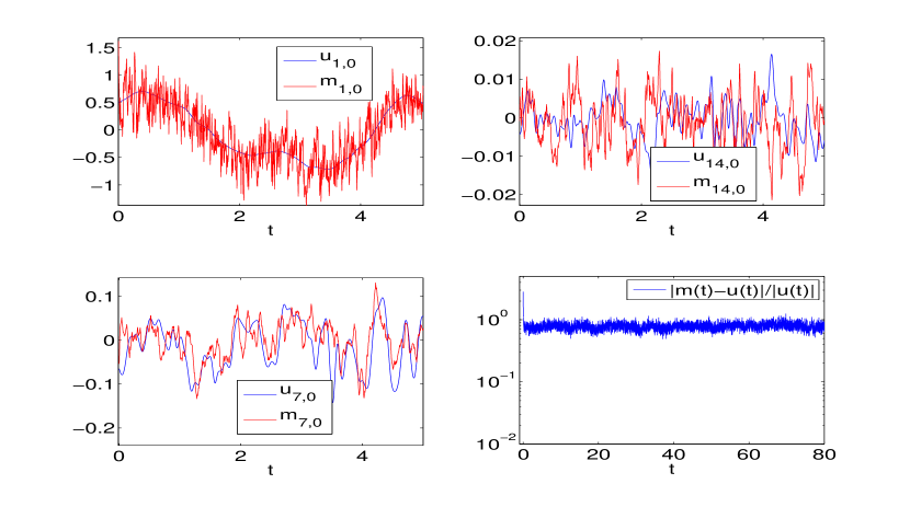
Figure 1: Trajectories of various modes of the estimator $\widehat{m}$ and the signal $u$ are depicted above for $\beta=0$ and $\sigma_{0}=0.05$, along with the total relative error in the $L^{2}$ norm, $|\widehat{m}-u|/|u|$.

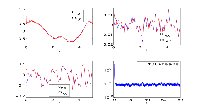
Figure 2: Trajectories of various modes of the estimator $\widehat{m}$ and the signal $u$ are depicted above for $\beta=0$ and $\sigma_{0}=0.005$, along with the relative error in the $L^{2}$ norm, $|\widehat{m}-u|/|u|$.

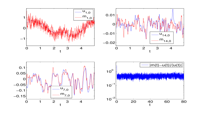
Figure 3: Trajectories of various modes of the estimator $\widehat{m}$ and the signal $u$ are depicted above for $\beta=1$ and $\sigma_{0}=0.05$, along with the relative error in the $L^{2}$ norm, $|\widehat{m}-u|/|u|$.

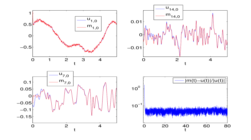
Figure 4: Trajectories of various modes of the estimator $\widehat{m}$ and the signal $u$ are depicted above for $\beta=1$ and $\sigma_{0}=0.005$, along with the relative error in the $L^{2}$ norm, $|\widehat{m}-u|/|u|$.

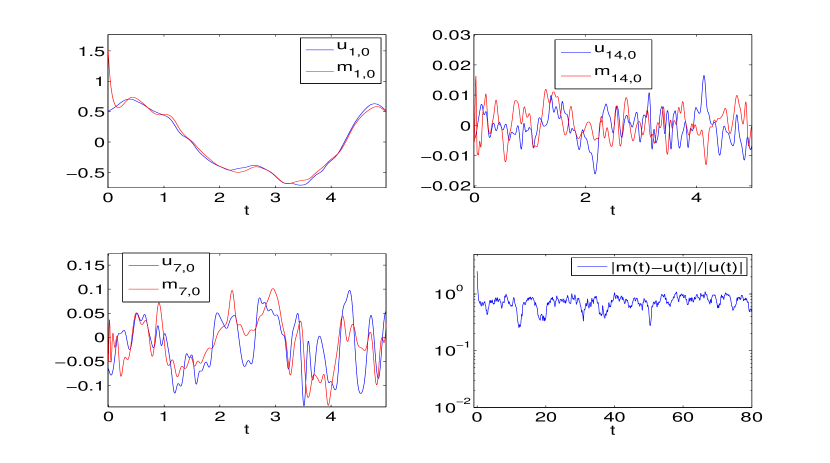
Figure 5: Trajectories of various modes of the estimator $\widehat{m}$ and the signal $u$ are depicted above for $\sigma_{0}=0$ and $\omega=10$, along with the relative error in the $L^{2}$ norm, $|\widehat{m}-u|/|u|$.

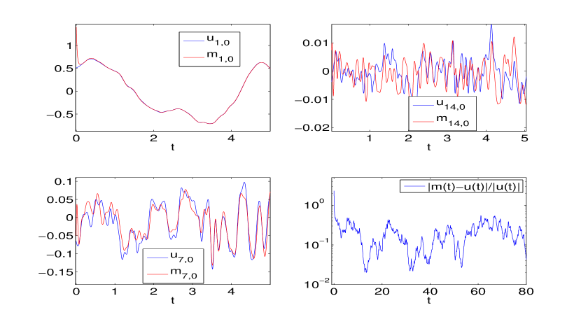
Figure 6: Trajectories of various modes of the estimator $\widehat{m}$ and the signal $u$ are depicted above for $\sigma_{0}=0$ and $\omega=30$, along with the relative error in the $L^{2}$ norm, $|\widehat{m}-u|/|u|$.

6.2 Forward Stability

This section will provide numerical evidence supporting Theorem 4.5. In order to investigate the stability of estimators we reproduce ensembles of solutions of equation (21), for a fixed realization of $W(t)$, and a family of initial conditions. We let $\beta=0$ throughout this section, and we always choose values of $\alpha$ which ensure that the trace class condition on the noise, $4\alpha+2\beta>1$, is satisfied.

Let $m^{(k)}(t)$ be the solution at time $t$ of (21) where the initial conditions are drawn from a Gaussian whose covariance is proportional to the model covariance: $m^{(k)}(0)\sim\mathcal{N}(0,30^{2}{\widehat{C}})$. First we consider $\alpha=1/2$. Figure 7 corresponds to parameters given in Fig. 1 of section 6.1. The top figure simply shows the ensemble of trajectories, while the bottom figure shows the convergence of $|m^{(k)}(t)-m^{(1)}(t)|/|m^{(1)}(t)|$ for $k>1$. Notice the trajectories converge to each other, indicating stability. But, the trajectories here do not converge to the truth (or driving signal). This is because the neighbourhood of the signal which bounds the estimators is not small. The next image, Fig. 8, shows results for the smaller value of $\sigma_{0}=0.005$ corresponding to Fig. 2 of section 6.1. Notice the rate of convergence of the trajectories to each other (bottom) is very similar to the previous case, indicating that there is again stability. However, this time the neighbourhood of the signal which bounds the estimators is small, and so they are indeed accurate. Fig. 9 shows the results for the larger value of $\alpha=1$ (still with $\beta=0$). In this case, there is no stability, i.e. the trajectories do not converge to each other (bottom), and also no convergence to the truth (bottom right of the top panels), although all trajectories do remain in a neighbourhood of the truth and the low wavevector modes converge (top left), so there is accuracy with a large bound. Furthermore, the distance of the trajectories from each other is similar to the distance from the truth, so the attractor in this case may be similar to the attractor of the underlying Navier-Stokes equation.

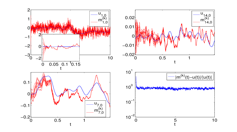
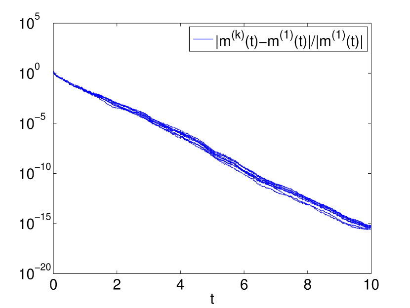
Figure 7: The above panels correspond to Fig. 1 from the text, except illustrating stability by an ensemble of estimators. The top set of panels are the same as in Fig. 1, while the bottom panel shows stability by convergence of the estimators to each other.

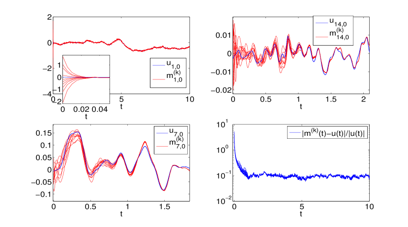
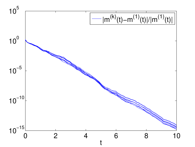
Figure 8: The above panels correspond to Fig. 2 from the text, except illustrating stability by an ensemble of estimators. The top set of panels are the same as in Fig. 2, while the bottom panel shows stability by convergence of the estimators to each other.

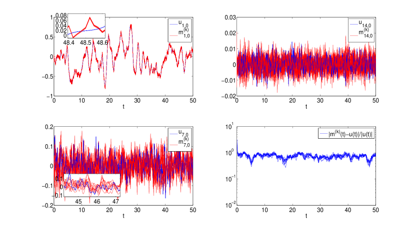
Figure 9: The above panels correspond to the same parameter values as above Fig. 8, except $\alpha=1$. Panels are the same. There is not stability in this case.

6.3 Pullback Accuracy and Stability

Finally, in this section, we illustrate Theorem 5.7. As the subtle nuance differences between forward and pullback accuracy and stability ellude standard numerical simulation, we do not feel it is appropriate to explore this in further detail numerically. So, this section will be brief. We include a single image illustrating the equivalence of the above experiments in Figures 8, 7, and 9 to the traditional notion of pullback attractor in the case that the attractor is a point: Figure 10.

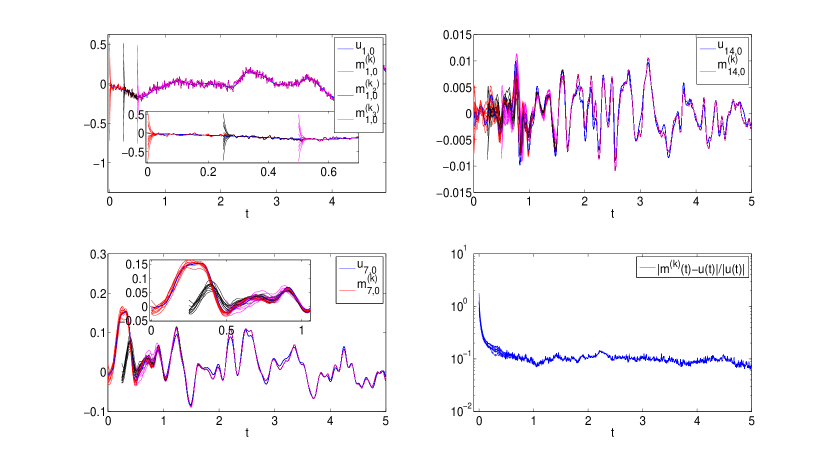
Figure 10: The same as Figure 8, except the initial ensemble is initiated at 3 separate times: $t_{1},t_{2},$ and $t_{3}$. Clearly the only relevant interval of time is for $t>t_{3}$. All trajectories converge to each other.

7 Conclusions

Data assimilation is important in a range of physical applications where it is of interest to use data to improve output from computational models. Analysis of the various algorithms used in practice is in its infancy. The work herein contains analysis of an algorithm, 3DVAR, which is prototypical of more complex Gaussian approximations that are widely used in applications. In particular we have studied the high frequency in time observation limit of 3DVAR, leading to a stochastic PDE. We have demonstrated mathematically how variance inflation, widely used by practitioners, stabilizes, and makes accurate, this filter, complementing the theory in [5] which concerns low frequency in time observations. It is to be expected that the analytical tools developed here and in [5] can be built upon to study more complex algorithms, such as the extended and ensemble Kalman filters, variants on which are used in operational weather forecasting. This will form a focus of our future work.

References

- [1] L. Arnold. Random Dynamical Systems. Springer, New York, 1998.
- [2] A. Bain and D. Crişan. Fundamentals of Stochastic Filtering. Springer Verlag, 2008.
- [3] A. Bennett. Inverse Modeling of the ocean and Atmosphere. Cambridge, 2002.
- [4] A. Beskos, D. Crisan, and A. Jasra. On the stability of sequential monte carlo methods in high dimensions. arXiv preprint arXiv:1103.3965, 2011.
- [5] CEA Brett, KF Lam, KJH Law, DS McCormick, MR Scott, and AM Stuart. Stability of filters for the Navier-Stokes equation. Arxiv preprint arXiv:1110.2527, 2011.
- [6] A. Carrassi, M. Ghil, A. Trevisan, and F. Uboldi. Data assimilation as a nonlinear dynamical systems problem: Stability and convergence of the prediction-assimilation system. Chaos: An Interdisciplinary Journal of Nonlinear Science, 18:023112, 2008.
- [7] A. Chorin, M. Morzfeld, and X. Tu. Implicit particle filters for data assimilation. Communications in Applied Mathematics and Computational Science, page 221, 2010.
- [8] P. Constantin and C. Foiaş. Navier-Stokes equations. University of Chicago Press, 1988.
- [9] H. Crauel, Debussche A., and F. Flandoli. Random attractors. J. Dynam. Differential Equations, 9:307–341, 1995.
- [10] H. Crauel and F. Flandoli. Attractor for random dynamical systems. Prob. Theory and Relat. Fields, 100:365–393, 1994.
- [11] G. Da Prato and J. Zabczyk. Ergodicity for infinite dimensional systems, volume 229. Cambridge Univ Pr, 1996.
- [12] G. Da Prato and J. Zabczyk. Stochastic equations in infinite dimensions. Cambridge Univ Pr, 2008.
- [13] A. Doucet, N. De Freitas, and N. Gordon. Sequential Monte Carlo methods in practice. Springer Verlag, 2001.
- [14] A. Es-Sarhir and W. Stannat. Improved moment estimates for invariant measures of semilinear diffusions in hilbert spaces and applications. J. Funct. Anal., 259(5):1248–1272, 2010.
- [15] G. Evensen. Data Assimilation: the Ensemble Kalman Filter. Springer Verlag, 2009.
- [16] F. Flandoli. Dissipativity and invariant measures for stochastic navier-stokes equations. NoDEA, Nonlinear Differ. Equ. Appl., 1(4):403–423, 1994.
- [17] F. Flandoli and D. Gatarek. Martingale and stationary solutions for stochastic navier-stokes equations. Probab. Theory Relat. Fields, 102(3):367–391, 1995.
- [18] F. Flandoli and B. Maslowski. Ergodicity of the 2-d navier-stokes equation under random perturbations. Commun. Math. Phys., 172(1):119–141, 1995.
- [19] M. Hairer and J.C. Mattingly. Ergodicity of the 2D Navier-Stokes equations with degenerate stochastic forcing. Annals of Mathematics, 164:993–1032, 2006.
- [20] J. Harlim and AJ Majda. Filtering nonlinear dynamical systems with linear stochastic models. Nonlinearity, 21:1281, 2008.
- [21] A.C. Harvey. Forecasting, Structural Time Series Models and the Kalman filter. Cambridge Univ Pr, 1991.
- [22] K. Hayden, E. Olson, and E.S. Titi. Discrete data assimilation in the Lorenz and 2d Navier-Stokes equations. Physica D: Nonlinear Phenomena, 2011.
- [23] E. Kalnay. Atmospheric modeling, data assimilation, and predictability. Cambridge Univ Pr, 2003.
- [24] P.E. Kloeden, E. Platen, and H. Schurz. Stochastic differential equations. Numerical Solution of SDE Through Computer Experiments, pages 63–90, 1994.
- [25] A.C. Lorenc. Analysis methods for numerical weather prediction. Quarterly Journal of the Royal Meteorological Society, 112(474):1177–1194, 1986.
- [26] A.J. Majda, J. Harlim, and B. Gershgorin. Mathematical strategies for filtering turbulent dynamical systems. Dynamical Systems, 27(2):441–486, 2010.
- [27] J.C. Mattingly. Exponential convergence for the stochastically forced navier-stokes equations and other partially dissipative dynamics. Communications in mathematical physics, 230(3):421–462, 2002.
- [28] E. Olson and E.S. Titi. Determining modes for continuous data assimilation in 2D turbulence. Journal of statistical physics, 113(5):799–840, 2003.
- [29] J. C. Robinson. Infinite-Dimensional Dynamical Systems. Cambridge Texts in Applied Mathematics. Cambridge University Press, Cambridge, 2001.
- [30] B. Schmalfuss. Bemerkungen zur zweidimensionalen stochastischen navier-stokes-gleichung. Math. Nachr., 131:19–32, 1987.
- [31] T. Snyder, T. Bengtsson, P. Bickel, and J. Anderson. Obstacles to high-dimensional particle filtering. Monthly Weather Review., 136:4629–4640, 2008.
- [32] T.J. Tarn and Y. Rasis. Observers for nonlinear stochastic systems. Automatic Control, IEEE Transactions on, 21(4):441–448, 1976.
- [33] R. Temam. Navier-Stokes Equations and Nonlinear Functional Analysis. Number 66. Society for Industrial Mathematics, 1995.
- [34] R. Temam. Infinite-Dimensional Dynamical Systems in Mechanics and Physics, volume 68 of Applied Mathematical Sciences. Springer-Verlag, New York, second edition, 1997.
- [35] R. Temam. Navier-Stokes equations. AMS Chelsea Publishing, Providence, RI, 2001.
- [36] Z. Toth and E. Kalnay. Ensemble forecasting at NCEP and the breeding method. Monthly Weather Review, 125:3297, 1997.
- [37] A. Trevisan and L. Palatella. Chaos and weather forecasting: the role of the unstable subspace in predictability and state estimation problems. International Journal of Bifurcation and Chaos, 21(12):3389–3415, 2011.
- [38] P.J. Van Leeuwen. Particle filtering in geophysical systems. Monthly Weather Review, 137:4089–4114, 2009.
- [39] PJ van Leeuwen. Nonlinear data assimilation in geosciences: an extremely efficient particle filter. Quarterly Journal of the Royal Meteorological Society, 136(653):1991–1999, 2010.