Fast evaluation of asymptotic waveforms
from gravitational perturbations

Abstract

In the context of blackhole perturbation theory, we describe both exact evaluation of an asymptotic waveform from a time series recorded at a finite radial location and its numerical approximation. From the user’s standpoint our technique is easy to implement, affords high accuracy, and works for both axial (Regge-Wheeler) and polar (Zerilli) sectors. Our focus is on the ease of implementation with publicly available numerical tables, either as part of an existing evolution code or a post-processing step. Nevertheless, we also present a thorough theoretical discussion of asymptotic waveform evaluation and radiation boundary conditions, which need not be understood by a user of our methods. In particular, we identify (both in the time and frequency domains) analytical asymptotic waveform evaluation kernels, and describe their approximation by techniques developed by Alpert, Greengard, and Hagstrom. This paper also presents new results on the evaluation of far-field signals for the ordinary (acoustic) wave equation. We apply our method to study late-time decay tails at null-infinity, “teleportation” of a signal between two finite radial values, and luminosities from extreme-mass-ratio binaries. Through numerical simulations with the outer boundary as close in as $r=30M$, we compute asymptotic waveforms with late-time $t^{-4}$ decay ($\ell=2$ perturbations), and also luminosities from circular and eccentric particle-orbits that respectively match frequency domain results to relative errors of better than $10^{-12}$ and $10^{-9}$. Furthermore, we find that asymptotic waveforms are especially prone to contamination by spurious junk radiation.

I Introduction

Asymptotic-waveform evaluation (AWE) is a long standing challenge in the computation of waves. Whether for acoustic, electromagnetic, or gravitational waves the goal is to identify the far-field or asymptotic signal radiated to future null infinity $\mathscr{I}^{+}$ using only knowledge of the solution on a truncated, spatially finite, computational domain. For the unit-speed ordinary wave equation, the far-field signal is $f(u,\theta,\phi)=\lim_{r\rightarrow\infty}r\psi(u,r,\theta,\phi)$, where $\psi(u,r,\theta,\phi)$ is a solution to the wave equation written with respect to retarded-time $u=t-r$ and spherical polar coordinates $(r,\theta,\phi)$. Continuing with this example, we view computation of $r_{\infty}\psi(u,r_{\infty},\theta,\phi)$ as AWE, so long as the evaluation radius $r_{\infty}$ can be taken arbitrarily large, even if ultimately finite. Indeed, for the ordinary wave equation the asymptotic signal and signal at $r_{\infty}=10^{15}$ are identical to about double precision machine epsilon (see Appendix A for the error estimate). The asymptotic signal we compute corresponds to observation on the timelike hyper-cylinder $r=r_{\infty}$. In the perturbative gravitational setting considered here, with $r_{\infty}=2M\left(1\times 10^{15}\right)$ in terms of the Schwarzschild mass $M$, such observations take place in the astrophysical zone Leaver ; Barack1999 ; Purrer:2004nq . An observation in the astrophysical zone is better approximated as taking place at $\mathscr{I}^{+}$ rather than future timelike infinity $i^{+}$ Zenginoglu:2008wc ; Leaver ; Purrer:2004nq ; Barack1999 . For this reason, and for clarity of exposition, throughout this paper we refer to such observations as taking place at $\mathscr{I}^{+}$.

Identifying the gravitational wave signal at $\mathscr{I}^{+}$ is of both theoretical and practical importance. Theoretically, in the context of asymptotically flat spacetimes Sachs Sachs:1962 identified the asymptotic metric factors corresponding to $f(u,\theta,\phi)$ for gravitation, and exploited this identification in his discussion of the radiative degrees of freedom for general relativity. Using Geroch’s calculation framework Geroch , Ashtekar and Streubel expanded on the Sachs approach in their fundamental analysis AshtekarStreubel of the symplectic structure of radiative modes and gravitational flux in general relativity. Several works DrayStreubel ; Dray ; Shaw then investigated the general charge integral (where the integration is over a two-surface “cut” of $\mathscr{I}^{+}$) corresponding to the Ashtekar-Streubel flux. The practical importance of AWE stems from the upcoming generation of advanced-sensitivity ground-based gravitational wave interferometer detectors (i.e., advanced LIGO, advanced Virgo, and KAGRA) KAGRA_web ; LIGO_web ; VIRGO_web ; GEO_web and anticipated space-based detectors like LISA LISA_web ; ESA_web . These instruments are well-modeled as idealized observers located at $\mathscr{I}^{+}$.

While the problem of AWE for gravitation shares difficulties with its counterparts for the ordinary wave and Maxwell equations, for example the slow fall-off of the waves (in our case metric perturbations) in powers of $1/r$, the gravitational problem is further complicated by the backscattering of waves, coordinate (gauge) issues, and non-linearities. For a perturbed Schwarzschild blackhole, covariant and gauge invariant approaches exist for the construction of “master functions” from the spacetime metric perturbations (see, for example, Sarbach:2001qq ; Martel_CovariantPert ; SopuertaLaguna ). In the asymptotic limit these master functions specify the gravitational waveform. Here we consider the wave equations which directly govern these master functions. In this perturbative setting, AWE is precisely the technique (perhaps extrapolation, for example) used to compute the master functions at arbitrarily large distances from the central blackhole. This paper introduces a new technique based on signal teleportation between two finite radial values.

A straightforward and longstanding approach to AWE in both full general relativity Pollney:2009yz ; Boyle2009 and perturbative settings Sundararajan:2007jg has been to record relevant field quantities at a variety of radii, perform a numerical fit, and then extrapolate to larger radii. However, the accuracy of this method ultimately relies on an Ansatz for the expected fall-off of the field with larger $r$, as well as recording field values at multiple and preferably large values of $r$ Pollney:2009ut . An alternative approach, known as Cauchy characteristic extraction, is to record geometrical data from a Cauchy evolution on a world-tube, which is later used as interior boundary data for a second characteristic evolution whose coordinates have been compactified to formally include $\mathscr{I}^{+}$ within the numerical grid Bishop ; Reisswig:2009us ; Babiuc:2010ze ; Winicour_LRR . When the background coordinates are fixed, $\mathscr{I}^{+}$ can be directly included within a Cauchy evolution by a geometric prescription using hyperboloidal methods Zenginoglu:2008wc ; Zenginoglu:2007jw ; Zenginoglu:2009hd ; Zenginoglu:2009ey ; Zenginoglu:2010cq ; Zenginoglu:2010zm ; Bernuzzi:2011aj ; Zenginoglu:2011zz . Another approach due to Abrahams and Evans shows how one may exactly evaluate asymptotic waveforms from gravitational multipoles for general relativity linearized about flat spacetime AE1 ; AE2 . This paper presents a new analytical and numerical method to evaluate asymptotic gravitational waveforms from perturbations of a non-spinning (Schwarzschild) blackhole. It also presents new results on the asymptotic signal evaluation problem for the acoustic (i.e. ordinary) wave equation. Our approach is most similar to that of Abrahams and Evans. Essentially, we reformulate their approach in a way which subsequently generalizes to blackhole perturbations. However, while our approach generalizes the Abrahams-Evans one to a curved background spacetime, we do not match their careful discussion of gauge issues.

For the Einstein equations linearized about Minkowski spacetime in the Lorenz gauge the trace-reversed metric perturbation obeys the flatspace (ordinary d’Alembertian) tensor wave equation. Therefore, these perturbations are akin to solutions of either the ordinary wave equation or the Maxwell equations; solutions characterized by the sharp Huygen’s principle and, therefore, which possess secondary lacunae PetropavlovskyTsynkov : given trivial initial data and an inhomogeneous source which is bounded in space and time, the solution vanishes on the intersection of all forward light cones whose vertices sweep over the support of the source. The secondary lacunae is a region of spacetime which is “dark” because all waves have already passed. Similar statements hold for the homogeneous case with non-trivial initial data of compact support. Actually, for the Maxwell case with certain sources, the solution may have a quasi-lacunae featuring a late-time static electric field PetropavlovskyTsynkov .

Wave propagation on a curved spacetime is more complicated due to the backscattering of waves off of curvature. Even within the relatively simple setting of perturbations of Schwarzschild blackholes, backscattering effects are present and the resulting late-time “tails” Price1972 ; DSS2011 have been extensively studied both theoretically and numerically. Backscattering confounds our intuitive sense of “outgoing” and “ingoing”; one might reasonably take the viewpoint that a partially backscattered wave has both outgoing and ingoing pieces. Nevertheless, for the linear master equations which describe perturbations of Schwarzschild blackholes, there is an unambiguous notion of “outgoing”, provided initial data of compact support. Away from the support of the initial data, Laplace transformation of a master equation (1) yields a homogeneous second-order ODE, which therefore has two linearly independent solutions, $\widehat{\Psi}^{(1)}(s,r)$ and $\widehat{\Psi}^{(-1)}(s,r)$, where $s$ is Laplace frequency. Here we have suppressed harmonic indices $(\ell,m)$ and assumed that the area radius $r$ is the independent spatial variable. We may assume that $\widehat{\Psi}^{(\pm 1)}(s,r)\sim\exp(\mp sr_{*})$ as $r,r_{*}\rightarrow\infty$, where $r_{*}$ is the Regge-Wheeler tortoise coordinate defined below. At a radial location beyond the support of the initial data, the frequency-domain solution has the form $\alpha(s)\widehat{\Psi}^{(+1)}(s,r)$, where the details of the initial data are buried in the coefficient $\alpha(s)$. Physically, this notion of “outgoing” would perhaps be better characterized as “asymptotically outgoing”. Nevertheless, provided the solution has this form, we can derive at a finite radius both time-domain boundary conditions Lau1 ; Lau2 ; Lau3 and an AWE procedure. The strategy in both cases is to write down the exact conditions/procedure in the frequency domain, and then accurately approximate this exact relationship in a fashion that allows for simple inversion under the inverse Laplace transform. For the case of boundary conditions, one approximates the exact Dirichlet-to-Neumann map as a rational function (in fact a sum of simple poles) along the axis of imaginary Laplace frequency (the inversion contour). The exact time-domain boundary condition is a history-dependent convolution, which maybe approximated to machine precision as a convolution involving a kernel given by a small sum of exponentials. As we show, this type of kernel effectively localizes the history dependence.

Our reformulation of the Abrahams-Evans procedure (and its generalization to curved spacetimes) features a similar history-dependent convolution involving a sum-of-exponentials time-domain kernel. Section III demonstrates that, in the (Laplace) frequency domain, an AWE kernel is exactly expressible as an “integral over boundary kernels”, thereby allowing us to leverage existing codes and knowledge for generating and approximating boundary kernels. While the construction of AWE kernels is computationally intensive, this is an offline cost. Once the kernel has been calculated, efficient and accurate AWE can be implemented within an existing code in a non-intrusive manner. Furthermore, AWE can be effected as a post-processing step on existing data recorded at a fixed radial location. Kernels used in this paper, as well as others, will be available at Kernel_web1 .

This paper is organized as follows. Section II provides a self-contained guide on using boundary and AWE kernels in either existing codes or data post-processing. Towards this end, Section II.3 considers the numerical evolution of late time tails from an approximate asymptotic signal which we find to decay at the rate predicted for $\ell=2$ perturbations at $\mathscr{I}^{+}$. Section III presents the theoretical underpinnings of both radiation boundary conditions and waveform teleportation, considering both wave propagation on flat (Minkowski) and Schwarzschild spacetime. For $\ell=2$, $3$, $64$ perturbations, Section IV.1 considers accurate signal teleportation to a finite (near-field) radial value. In Section IV.2 we apply our method to compute gravitational waveforms and luminosities from extreme mass ratio binary systems, finding excellent agreement with frequency domain computations. In these studies we have observed that spurious junk radiation is problematic for accurate $\mathscr{I}^{+}$ computations. Finally, we conclude in Section V by discussing open issues, both theoretical and practical.

II Implementation how-to guide

Our aim in this section is not to give a derivation of our AWE method. Rather, adopting the simplest possible evolution scheme and coordinates, we focus on how AWE is implemented. By presenting an implementation of our AWE method for a simple scheme, we hope to convey the key points to the reader, who will then grasp how to implement the method within their own evolution scheme. Since our implementation of AWE relies on certain radiation boundary conditions (RBC), themselves essential when working on a spatially finite domain, we first describe how to implement these within our simple scheme. Here we do not discuss our RBC and AWE methods for different background coordinate systems (i.e. Kerr-Schild or hyperboloidal foliations), but return to this issue in Appendix C.

Multipole gravitational perturbations of a Schwarzschild blackhole are described by the Regge-Wheeler (axial) and Zerilli (polar) formalisms RW ; ZER . In geometric units the corresponding “master” wave equations have the form

$$\frac{\partial^{2}\Psi}{\partial t^{2}}-\frac{\partial^{2}\Psi}{\partial r_{*}^{2}}+V^{\mathrm{RW,Z}}(r)\Psi=S,$$ (1)

where $S(t,r)$ is a possible source and in terms of the blackhole mass $M$ the Regge-Wheeler tortoise coordinate is $r_{*}=r+2M\log(\frac{1}{2}M^{-1}r-1)$, which we also denote by $x$. Until Section IV.2, we alway choose $S=0$ for the source. Expressions for the Zerilli $V^{\mathrm{Z}}(r)$ and Regge-Wheeler $V^{\mathrm{RW}}(r)$ potentials are given in, for example, Eqs. (2) and (3) of Ref. FHL . Both potentials depend on the orbital angular index $\ell$. We have suppressed this index on $V(r)$, as well as the orbital and azimuthal indices $(\ell,m)$ on the mode $\Psi$ and source $S$.

II.1 Simple evolution algorithm with RBC

Most numerical schemes for evolution of (1) employ some form of “auxiliary variables”, for example the variables $\Psi,\Pi\equiv-\partial_{t}\Psi,\Phi\equiv\partial_{x}\Psi$. However, for transparency here we use “characteristic variables”:

$$\Psi,\qquad W=-\Pi-\Phi,\qquad X=-\Pi+\Phi,$$ (2)

for which the evolution equations are

$$\partial_{t}\Psi=\frac{1}{2}(W+X),\quad\partial_{t}W=-\partial_{x}W-V(r(x))\Psi,\quad\partial_{t}X=\partial_{x}X-V(r(x))\Psi.$$ (3)

These equations show that $W$ propagates left-to-right ($\nearrow$) and $X$ propagates right-to-left ($\nwarrow$). While from the theoretical standpoint we prefer to view fields, for example $\Psi(t,r)$, as depending spatially on $r$, from a computationally standpoint we discretize Eqs. (3) in $x$. Therefore, suppose the computational domain is the interval $[a,b]$ in tortoise coordinate $x$, corresponding to the interval $[r_{a},r_{b}]$ in Schwarzschild radius $r$. Boundary conditions must be specified for $W$ at $x=a$ and for $X$ at $x=b$. We discretize (3) using first-order upwind stencils in space, and the forward Euler method in time. Respectively, let $\{t_{n}\}$ and $\{x_{k}\}_{k=0}^{K}$ denote uniformly spaced temporal and spatial grid points such that $\Delta x=x_{k+1}-x_{k}$. Moreover, let $V_{k}\equiv V(r(x_{k}))$ and $\Psi^{n}_{k}\simeq\Psi(t_{n},r(x_{k}))$, with the same notation for the other fields. Then the scheme for updating the fields at all $x_{k}$ from time $t_{n}$ to time $t_{n+1}=t_{n}+\Delta t$ is given by Algorithm 1.

Algorithm 1 Finite difference scheme for Eqs. (3)

1:$\Psi^{n+1}_{0}=\Psi^{n}_{0}+(\Delta t/2)\big{[}W^{n}_{0}+X^{n}_{0}\big{]}$

2:$W^{n+1}_{0}=W_{a}^{n+1}$ $\triangleright$ Boundary condition at $a$

3:$X^{n+1}_{0}=X^{n}_{0}+(\Delta t/\Delta x)\big{(}X^{n}_{1}-X^{n}_{0}\big{)}-\Delta tV_{0}\Psi^{n}_{0}$

4:for $k=1\text{ \bf{to} }K-1$ do

5:            $\Psi^{n+1}_{k}=\Psi^{n}_{k}+(\Delta t/2)\big{[}W^{n}_{k}+X^{n}_{k}\big{]}$

6:            $W^{n+1}_{k}=W^{n}_{k}-(\Delta t/\Delta x)\big{(}W^{n}_{k}-W^{n}_{k-1}\big{)}-\Delta tV_{k}\Psi^{n}_{k}$

7:            $X^{n+1}_{k}=X^{n}_{k}+(\Delta t/\Delta x)\big{(}X^{n}_{k+1}-X^{n}_{k}\big{)}-\Delta tV_{k}\Psi^{n}_{k}$

8:end for

9:$\Psi^{n+1}_{K}=\Psi^{n}_{K}+(\Delta t/2)\big{(}W^{n}_{K}+X^{n}_{K}\big{)}$

10:$W^{n+1}_{K}=W^{n}_{K}-(\Delta t/\Delta x)\big{(}W^{n}_{K}-W^{n}_{K-1}\big{)}-\Delta tV_{K}\Psi^{n}_{K}$

11:$X^{n+1}_{K}=X_{b}^{n+1}$ $\triangleright$ Boundary condition at $b$

To complete the scheme, we must specify both $W_{a}^{n}\simeq W(t_{n},r_{a})$ and $X_{b}^{n}\simeq X(t_{n},r_{b})$ as functions of (discrete) time. So long as $a\ll 0$, the inner boundary value of the potential $V(r)$ near $r=r_{a}$ is zero to machine precision, and the Sommerfeld boundary condition $W_{a}^{n}=0,\forall n$ is highly accurate. The RBC at $x=b$ is determined by a Laplace convolution,

$$X(t,r_{b})=\frac{f(r_{b})}{r_{b}}\int_{0}^{t}\Xi(t-t^{\prime},r_{b})\Psi(t^{\prime},r_{b})dt^{\prime},$$ (4)

where $f(r)=1-2M/r$ and the boundary time-domain kernel is

$$\Xi(t,r_{b})=\sum_{q=1}^{d}\frac{\gamma_{q}(\rho_{b})}{2M}\Xi_{q}(t,r_{b}),\qquad\Xi_{q}(t,r_{b})=\exp\left(\frac{\beta_{q}(\rho_{b})t}{2M}\right).$$ (5)

The parameters $\{(\gamma_{q}(\rho_{b}),\beta_{q}(\rho_{b}))\}_{q=1}^{d}$ depend on the rescaled boundary radius $\rho_{b}=(2M)^{-1}r_{b}$ (as well as the orbital index $\ell$ which is suppressed) and they are listed in numerical tables, such as those given in the Appendix D. Some of the parameters $\{(\gamma_{q},\beta_{q})\}_{q=1}^{d}$ are complex, but the kernel $\Xi(t,r_{b})$ is real. We stress that, insofar as implementation of the convolution (4) is concerned, the origin of these numbers is unimportant. Defining, for example, $\Psi_{b}(t)=\Psi(t,r_{b})$, we write (4) as $X_{b}(t)=r_{b}^{-1}f(r_{b})(\Xi(\cdot,r_{b})*\Psi_{b})(t)$. With a similar notation, the constituent convolution $(\Xi_{q}*\Psi_{b})\equiv(\Xi_{q}(\cdot,r_{b})*\Psi_{b})(t)$ obeys an ODE at the boundary,

$$\frac{d}{dt}(\Xi_{q}*\Psi_{b})=\big{[}(2M)^{-1}\beta_{q}(\Xi_{q}*\Psi_{b})+\Psi_{b}\big{]}.$$ (6)

These $d$ ODE can be integrated along side the system (3). Indeed, we define $(\Xi_{q}*\Psi_{b})^{n}\simeq(\Xi_{q}*\Psi_{b})(t_{n})$ and complete our scheme as follows.

Algorithm 2 Finite difference scheme for Eqs. (3) with RBC

1:for $q=1\text{ \bf{to} }d$ do $\triangleright$ First update constituent convolutions

2:            $(\Xi_{q}*\Psi_{b})^{n+1}=(\Xi_{q}*\Psi_{b})^{n}+\Delta t\big{[}(2M)^{-1}\beta_{q}(\Xi_{q}*\Psi_{b})^{n}+\Psi^{n}_{K}\big{]}$

3:end for

4:$X_{b}^{n+1}=(2Mr_{b})^{-1}f(r_{b})\sum_{q=1}^{d}\gamma_{q}(\Xi_{q}*\Psi_{b})^{n+1}$

5:$W_{a}^{n+1}=0$

6:Run Algorithm 1 with $W_{a}^{n+1}$ and $X_{b}^{n+1}$ given by above values.

II.2 Evaluation of the asymptotic waveform

Our approach to AWE is similar to the described implementation of radiation boundary conditions. We introduce new parameters $\{(\gamma^{E}_{q}(\rho_{b},\rho_{\infty}),\beta^{E}_{q}(\rho_{b},\rho_{\infty}))\}_{q=1}^{d^{E}}$ and a new kernel

$$\Xi^{E}(t,r_{b},r_{\infty})=\sum_{q=1}^{d^{E}}\frac{\gamma^{E}_{q}(\rho_{b},\rho_{\infty})}{2M}\Xi^{E}_{q}(t,\rho_{b},\rho_{\infty}),\qquad\Xi^{E}_{q}(t,\rho_{b},\rho_{\infty})=\exp\left(\frac{\beta^{E}_{q}(\rho_{b},\rho_{\infty})t}{2M}\right).$$ (7)

The parameters $\{(\gamma^{E}_{q}(\rho_{b},\rho_{\infty}),\beta^{E}_{q}(\rho_{b},\rho_{\infty})\}_{q=1}^{d^{E}}$ also depend on $\ell$, but this dependence has been suppressed. The $E$ here stands for “evaluation” and differentiates this kernel from the RBC one. This evaluation kernel enacts teleportation (the term is defined in Section III) of the waveform from the boundary radius $r_{b}=2M\rho_{b}$ to the evaluation radius $r_{\infty}=2M\rho_{\infty}\gg r_{b}$ (from $b$ to $x_{\infty}$ in tortoise coordinate). As discussed below, the choice $r_{\infty}=\infty$ is formally possible (see Sec. V); however, in this paper $r_{\infty}$ is an arbitrarily large, albeit finite, radius. To ensure the signals recovered at $r_{\infty}$ and $\mathscr{I}^{+}$ are identical to about machine precision, we choose $r_{\infty}=2M(1\times 10^{15})$ for double precision simulations, and would choose $r_{\infty}=2M(1\times 10^{30})$ for quadruple precision simulations. We then approximate the asymptotic waveform as

$$\Psi_{\infty}(t):=\Psi(t+(x_{\infty}-b),r_{\infty})\simeq\int_{0}^{t}\Xi^{E}(t-t^{\prime},r_{b},r_{\infty})\Psi(t^{\prime},r_{b})dt^{\prime}+\Psi(t,r_{b}).$$ (8)

The offset by $\Psi(t,r_{b})$ in this formula stems from a technicality explained in Section III.1. As before, this formula can be implemented through integration of ODE at the boundary, only now these ODE are not coupled to the numerical evolution. With $(\Xi_{q}^{E}*\Psi_{b})^{n}\simeq(\Xi_{q}^{E}(\cdot,r_{b})*\Psi_{b})(t_{n})$ and $\Psi_{\infty}^{n}\simeq\Psi_{\infty}(t_{n})$, the algorithm using forward Euler is as follows.

Algorithm 3 Evaluation of asymptotic waveform, placed after field update

1:for $q=1\text{ \bf{to} }d^{E}$ do

2:            $(\Xi_{q}^{E}*\Psi_{b})^{n+1}=(\Xi_{q}^{E}*\Psi_{b})^{n}+\Delta t\big{[}(2M)^{-1}\beta_{q}^{E}(\Xi_{q}^{E}*\Psi_{b})^{n}+\Psi^{n}_{K}\big{]}$

3:end for

4:$\Psi_{\infty}^{n+1}=(2M)^{-1}\sum_{q=1}^{d}\gamma_{q}^{E}(\Xi_{q}^{E}*\Psi_{b})^{n+1}+\Psi^{n+1}_{K}$

The following condition would yield particularly efficient AWE:

$$d^{E}=d,\quad\beta^{E}_{q}(\rho_{b},\rho_{\infty})=\beta_{q}(\rho_{b}),\quad\forall q,\text{ (preferred, but perhaps {\em not} possible).}$$ (9)

Indeed, integration of the same ODE (6) at the boundary would then determine both the RBC and AWE. In this case, steps 1 through 3 of Algorithm 3 have already been carried out in Algorithm 2. However, the assumption in (9) may not always be possible, and even when possible appears to yield less accurate teleportation kernels. We have constructed $\ell=2$ AWE kernels which satisfy (9) (an example is given in the Appendix D); however, relative to our best kernels, they indeed yield less accuracy. Moreover, we have been unable to achieve (9) for $\ell=64$ teleportation kernels. Therefore, in this paper we will not assume (9).

Remark. If $\Psi$ is itself complex (as is the case in applications), then round-off issues will lead to mixing of the real and imaginary parts in the simple algorithms above. In this case, we advocate splitting the complex exponentials which make up $\Xi$ and $\Xi^{E}$ into manifestly real expressions involving sine and cosine terms. Such splitting amounts to extra bookkeeping, but hardly complicates the above treatment.

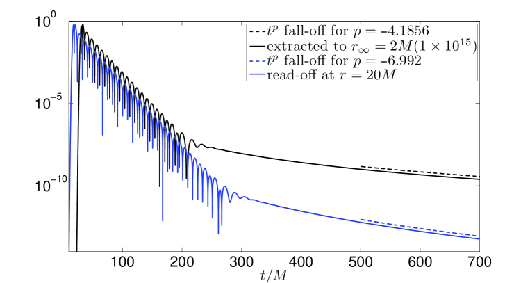
Figure 1: Quasinormal ringing and decay tails. Each dashed curve corresponds to power law decay, with the indicated rate determined by a least squares fit of the field over the time window $[500,700]M$. The time shift for the asymptotic waveform has not been included.

II.3 Numerical experiment: quasinormal ringing and decay tails

Section IV documents the results of several numerical experiments which validate and test our methods. This subsection also describes a numerical experiment, although here with the goal of providing further assistance toward implementation. An interested reader might first repeat the experiment described below.

We consider the $\ell=2$ Regge-Wheeler equation and Gaussian initial data

$$\Psi=e^{-[2-x/(2M)]^{2}},\quad\Phi=\frac{4M-x}{2M^{2}}e^{-[2-x/(2M)]^{2}},\quad\Pi=\Phi(0,r(x)).$$ (10)

For this experiment the computational $x$-domain is $[a,b]$, where $a=-200M$ and $b=30M+2M\log(14)$ corresponds to $\rho_{b}=r_{b}/(2M)=15$. We evolve the data (10) until time $t=600M$, with a Sommerfeld boundary condition at $x=a$ and the convolution boundary condition (4) at $x=b$. Table 3 in Appendix D lists the 26 pole RBC kernel $\Xi$ used for this convolution. Instead of Algorithm 1 we use a multidomain Chebyshev collocation method with classical Runge Kutta 4 as the timestepper.

During the simulation we record as a time series both the field $\Psi(t,20M)$ and $\Psi(t,r_{b})$. Through the convolution (8) determined by Table 5 in Appendix D, the field $\Psi(t,r_{b})$ is teleported from $r_{b}=30M$ to $r_{\infty}=2M(1\times 10^{15})$ providing a time series which approximates the asymptotic waveform $\Psi_{\infty}(t)$. In absolute value $\Psi(t,20M)$ (solid blue line) and $\Psi_{\infty}(t)$ (solid black line) are depicted in Fig. 1. The time shift for the teleported waveform has not been included, and we have chosen to record $\Psi(t,20M)$ at $r=20M<r_{b}$ only to ensure that the time series in the plot do not lie on top of each other at early times. These series exhibit the phenomena of quasinormal ringing and late time decay tails. Each dashed curve in the figure corresponds to power law decay, with the indicated rate determined by a least squares fit based on the numerical decay of the field over dashed curve’s time window. The decay rates $p=-7$ and $p=-4$ are respectively the theoretical predictions gundlach1994late ; Barack:1998bw ; Zenginoglu:2009ey for a finite radius and $\mathscr{I}^{+}$.

Figure 2 shows the decay rate computed from $p=\partial_{\mathrm{ln}t}\mathrm{ln}|\Psi_{\infty}(t)|$ for the teleported signal with the evolution carried out to $t=25000M$. As a post-processing procedure, generation of this figure from existing data would take a few seconds. The decay for the teleported signal asymptotically approaches $p=-4$ at later times. The teleported pulse corresponds to a time series recorded along the wordline $(t_{\mathrm{obs}}+x_{\infty}-b,r_{\infty})$ by an observer safely within the astrophysical zone. Here $x_{\infty}-b$ is the time shift, and the astrophysical zone is defined as the region where $t_{\mathrm{obs}}\ll r_{\infty}$, with $t_{\mathrm{obs}}$ the time elapsed after the pulse’s leading edge passes our fictitious observer Leaver ; Purrer:2004nq ; Barack1999 . Since an observation in the astrophysical zone is well approximated as taking place at $\mathscr{I}^{+}$, the observed $-4$ decay rate is expected. For very late times the decay rate should settle towards $-7$, although extended precision might be necessary to capture the transition.

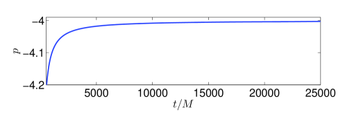
Figure 2: Tail decay rate for the teleported signal. The rate $p$ for $\Psi_{\infty}(t)\propto t^{p}$ has been computed using logarithmic difference quotients based on $\partial_{\ln t}\ln|\Psi_{\infty}(t)|$.

III Theoretical discussion

To fix ideas and motivate the new method, the next subsection describes AWE for flatspace multipole solutions of the ordinary 3+1 wave equation, formally the $M=0$ case of Eq. (1). Formulas derived in the next subsection motivate similar ones given for blackhole perturbations in subsection III.2.

III.1 Flatspace waves

This subsection describes (i) outgoing multipole solutions to the flatspace radial wave equation, (ii) the exact RBC obeyed by outgoing multipoles, and (iii) the relationship between this RBC and AWE for outgoing multipoles. Throughout this subsection, we often choose $\ell=2$ as a representative example, but similar (obvious) results hold for any multipole-order $\ell$.

III.1.1 Structure of outgoing and ingoing flatspace multipoles

General outgoing ($\epsilon=1$) and ingoing ($\epsilon=-1$) order-$\ell$ multipole solutions of the 3+1 wave equation $(-\partial_{t}^{2}+\partial_{x}^{2}+\partial_{y}^{2}+\partial_{z}^{2})\psi=0$ have the form (see, for example, Refs. Burke ; gundlach1994late )

$$\psi(t,x,y,z)=\frac{1}{r}\Psi^{(\epsilon)}_{\ell}(t,r)Y_{\ell m}(\theta,\phi),\quad\Psi^{(\epsilon)}_{\ell}(t,r)=\sum_{k=0}^{\ell}\frac{\epsilon^{k}}{r^{k}}c_{\ell k}f^{(\ell-k)}(t-\epsilon r),\quad c_{\ell k}=\frac{1}{2^{k}k!}\frac{(\ell+k)!}{(\ell-k)!},$$ (11)

where we have suppressed the azimuthal index $m$ on the “mode” $\Psi^{(\epsilon)}_{\ell}(t,r)$. In Eq. (11) $f^{(p)}(u)$ is the $p$th derivative of an underlying function $f(u)$ of retarded time $u=t-r$, and similarly for $f^{(p)}(v)$, where $v=t+r$ is advanced time. In (11) we view $(x,y,z)$ as place holders for $(r\sin\theta\cos\phi,r\sin\theta\sin\phi,r\cos\theta)$. For both $\epsilon=\pm 1$ cases the mode obeys the flatspace radial wave equation

$$\frac{\partial^{2}\Psi^{(\epsilon)}_{\ell}}{\partial t^{2}}-\frac{\partial^{2}\Psi^{(\epsilon)}_{\ell}}{\partial r^{2}}+\frac{\ell(\ell+1)}{r^{2}}\Psi^{(\epsilon)}_{\ell}=0,$$ (12)

and, specializing to the representative example, the outgoing quadrupole is

$$\Psi^{(1)}_{2}(t,r)=f^{\prime\prime}(t-r)+\frac{3}{r}f^{\prime}(t-r)+\frac{3}{r^{2}}f(t-r).$$ (13)

We are interested in the $(\epsilon=1)$ outgoing case, and so now write $\Psi_{\ell}(t,r)$ to mean $\Psi^{(1)}_{\ell}(t,r)$.

Given a fixed radius $r_{b}$ which specifies the outer boundary, consider the following assumption on the initial data (one of compact support):

$$\Psi_{\ell}(0,r)=0=(\partial_{t}\Psi_{\ell})(0,r),\qquad r>r_{b}-\delta,\qquad\text{for any small }\delta>0.$$ (14)

Provided that (14) holds, in the region $r\geq r_{b}$ Laplace transformation of an outgoing mode $\Psi_{\ell}(t,r)$ yields

$$\widehat{\Psi}_{\ell}(s,r)=a(s)s^{\ell}e^{-sr}W_{\ell}(sr),\quad W_{\ell}(z)=\sum_{k=0}^{\ell}\frac{c_{\ell k}}{z^{k}},$$ (15)

where $z=sr$ and

$$a(s)\equiv e^{sr}\int_{0}^{\infty}e^{-st}f(t-r)dt=\int_{-r_{b}}^{\infty}e^{-su}f(u)du.$$ (16)

Notice that $a(s)$ is indeed independent of $r$. For the quadrupole case, we have

$$\widehat{\Psi}_{2}(s,r)=a(s)s^{2}e^{-sr}W_{2}(sr),\qquad W_{2}(z)=1+\frac{3}{z}+\frac{3}{z^{2}}$$ (17)

[compare this expression with Eq. (13)].

To obtain (15) and (16), we have used (14) as follows. First consider the Laplace transform of $f^{(\ell-k)}(t-r)$ which appears in (11). Repeated integration by parts generates $t=0$ boundary terms of the form $f^{(\ell-k-p)}(-r)$ for $1\leq p\leq\ell-k$. All such terms vanish, as can be shown by the following identity:

$$f(t-r)=(-1)^{\ell}\frac{2^{\ell}}{(2\ell)!}\left[r^{2}\left(\partial_{t}+\partial_{r}\right)\right]^{\ell}\Psi_{\ell}(t,r).$$ (18)

Since the initial data $\Psi_{\ell}$ and $\partial_{t}\Psi_{\ell}$ vanishes on an open spatial neighborhood of the spatial point with coordinate $r\geq r_{b}$, in fact $\Psi_{\ell}$ vanishes in an open spacetime neighborhood of the spacetime point with coordinates $(0,r)$. Therefore, all derivatives of $\Psi_{\ell}$ vanish in the same neighborhood, which implies $f^{(\ell-k-p)}(-r)=0$. This implication stems from repeated differentiation of (18) with $t=0$ enforced afterward.

The previous argument establishes that

$$\int^{\infty}_{0}e^{-st}f^{(\ell-k)}(t-r)dt=s^{\ell-k}e^{-sr}\int^{\infty}_{-r}e^{-su}f(u)du.$$ (19)

The lower limit $-r$ of integration can now be replaced with $-r_{b}$. Indeed, (14) implies that $\Psi(t,r)=0$ for $0\leq t<\delta+(r-r_{b})$ and $r\geq r_{b}$. Using (18), we conclude that $f(u)=0$ for $-r\leq u\leq-r_{b}$. Therefore, the right-hand side of the last equation is $a(s)s^{\ell-k}e^{-sr}$.

III.1.2 Radiation boundary conditions for flatspace multipoles

We continue to derive expressions for $r\geq r_{b}$ where the assumption (14) of compact support holds. The explicit expression (15) for $\widehat{\Psi}_{\ell}(s,r)$ determines an exact frequency-domain boundary condition

$$s\widehat{\Psi}_{\ell}(s,r)+\partial_{r}\widehat{\Psi}_{\ell}(s,r)=\frac{1}{r}\widehat{\Omega}_{\ell}(s,r)\widehat{\Psi}_{\ell}(s,r),$$ (20)

where the frequency-domain radiation kernel $\widehat{\Omega}_{\ell}(s,r)$ defines the Sommerfeld residual. Indeed, the operator on the left-hand of (20) corresponds to the Sommerfeld operator $\partial_{t}+\partial_{r}$ in the time-domain. If $\ell=0$, then $\widehat{\Omega}_{\ell}(s,r)=0$; otherwise a simple computation based on Eqs. (15,20) shows that the frequency-domain kernel is given by (with the prime indicating differentiation in argument):

$$\widehat{\Omega}_{\ell}(s,r)\equiv sr\frac{W^{\prime}_{\ell}(sr)}{W_{\ell}(sr)}=\sum_{k=1}^{\ell}\frac{b_{\ell,k}/r}{s-b_{\ell,k}/r},$$ (21)

where $\{b_{\ell,k}:1\leq k\leq\ell\}$ are the roots of $W_{\ell}(z)$, all of which are simple. For the quadrupole case

$$\widehat{\Omega}_{2}(s,r)=\frac{z_{+}/r}{s-z_{+}/r}+\frac{z_{-}/r}{s-z_{-}/r},\quad z_{\pm}=-\frac{3}{2}\pm\mathrm{i}\frac{\sqrt{3}}{2},$$ (23)

where $z_{+}=b_{2,1}$ and $z_{-}=b_{2,2}$ solve $W_{2}(z_{\pm})=0$.

The time-domain RBC is the inverse Laplace transform of (20), i.e. the Laplace convolution GroteKeller1 ; GroteKeller2 ; Sofronov1 ; Sofronov2 ; AGH

$$\partial_{t}\Psi_{\ell}+\partial_{r}\Psi_{\ell}=\frac{1}{r}\int_{0}^{t}\Omega_{\ell}(t-t^{\prime},r)\Psi_{\ell}(t^{\prime},r)dt^{\prime},\quad\Omega_{\ell}(t,r)=\sum_{k=1}^{\ell}\frac{b_{\ell,k}}{r}\exp\left(\frac{b_{\ell,k}t}{r}\right).$$ (24)

Subject to our assumption (14) of compact support, the outgoing multipole [$\epsilon=1$ in Eq. (11)] obeys Eq. (24) exactly, as can also be shown via direct calculation using repeated integration by parts; see Appendix B. If, on the other hand, assumption (14) does not hold, then Eq. (24) is violated, but only by terms which decay exponentially fast in $t$; again, see Appendix B.

III.1.3 Asymptotic waveform evaluation and teleportation for flatspace multipoles

For a generic outgoing solution, it is possible to recover the profile function $f(t-r)$ and asymptotic waveform

$$\Psi_{\ell}(t,r)\sim f^{(\ell)}(t-r),\qquad r\rightarrow\infty,$$ (25)

via data recorded solely at a finite and fixed radial location, again taken as $r=r_{b}$. Let us consider the $\ell=2$ case as a concrete example. Generalization to higher $\ell$ is straightforward. Equation (13) suggests that we solve the ODE initial value problem

$$y^{\prime\prime}+\frac{3}{r}y^{\prime}+\frac{3}{r^{2}}y=\Psi_{2}(t,r),\qquad y(0)=0=y^{\prime}(0),\qquad(\ell=2\text{ problem})$$ (26)

in which case $f(u)=y(u+r)$.

In a pioneering series of papers AE1 ; AE2 , Abrahams and Evans showed how the above procedure carries over to the theory of gravitational multipoles for general relativity linearized about flat spacetime. We now re-examine the basic idea behind Abrahams-Evans AWE from the standpoint of Laplace convolution, and will consider two kernels: one $\Theta_{\ell}$ for evaluation of the underlying function $f(u)$ and another $\Phi_{\ell}$ more suited for evaluation of the waveform $f^{(\ell)}(u)$. Our implementations have mostly relied on the $\Phi_{\ell}$ kernel.

Continuing with the $\ell=2$ example, we introduce a frequency-domain profile evaluation kernel $\widehat{\Theta}_{2}(s,r)$ tailored to satisfy

$$\widehat{\Theta}_{2}(s,r)\widehat{\Psi}_{2}(s,r)=a(s)e^{-sr}=\widehat{y}(s).$$ (27)

That is, the product of $\widehat{\Theta}_{2}(s,r)$ and $\widehat{\Psi}_{2}(s,r)$ is $\int_{0}^{\infty}e^{-st}f(t-r)dt$ [cf. Eq. (16)]. Comparison with (17) immediately shows that

$$\widehat{\Theta}_{2}(s,r)=\frac{1}{s^{2}W_{2}(sr)}=\frac{\mathrm{i}r}{\sqrt{3}}\left[\frac{1}{s-z_{-}/r}-\frac{1}{s-z_{+}/r}\right].$$ (28)

The corresponding time-domain profile evaluation kernel is

$$\Theta_{2}(t,r)=\frac{\mathrm{i}r}{\sqrt{3}}\left[\exp\left(\frac{z_{-}t}{r}\right)-\exp\left(\frac{z_{+}t}{r}\right)\right],$$ (29)

and $y(t)=(\Theta_{2}(\cdot,r)*\Psi_{2}(\cdot,r))(t)$ solves the Abrahams-Evans initial value problem (26). Essentially the same arguments show that the order-$\ell$ profile evaluation kernel is

$$\widehat{\Theta}_{\ell}(s,r)=\frac{1}{s^{\ell}W_{\ell}(sr)}.$$ (30)

Despite appearances, the kernel is regular at $s=0$. For example, $1/W_{2}(sr)\sim(sr)^{2}/3$, and in general $1/W_{\ell}(sr)\sim(sr)^{\ell}/c_{\ell\ell}$, as $s\rightarrow 0$.

Direct evaluation of the asymptotic waveform is also possible. Teleportation by a positive shift $r_{2}-r_{1}$ means conversion of $\Psi(t,r_{1})$ to $\Psi(t+(r_{2}-r_{1}),r_{2})$, and it might correspond to a small finite shift $r_{2}-r_{1}$. However, when $r_{2}$ is suitably large, we write $r_{\infty}$ for $r_{2}$ and view teleportation as an AWE procedure (in which case typically $r_{1}=r_{b}$, and it is the boundary waveform $\Psi(t,r_{b})$ which is teleported). Teleportation is accomplished with a frequency-domain teleportation kernel

$$\widehat{\Phi}_{\ell}(s,r_{1},r_{2})=-1+\frac{W_{\ell}(sr_{2})}{W_{\ell}(sr_{1})}$$ (31)

rigged to satisfy

$$e^{s(r_{2}-r_{1})}\widehat{\Psi}_{\ell}(s,r_{2})=\widehat{\Phi}_{\ell}(s,r_{1},r_{2})\widehat{\Psi}_{\ell}(s,r_{1})+\widehat{\Psi}_{\ell}(s,r_{1}).$$ (32)

We have included the $-1$ factor in (31) to ensure that $\widehat{\Phi}_{\ell}(s,r_{1},r_{2})$ has a well-defined inverse Laplace transform $\Phi_{\ell}(t,r_{1},r_{2})$. In the time domain we recover the desired property

$$\Psi_{\ell}(t+(r_{2}-r_{1}),r_{2})=(\Phi_{\ell}(\cdot,r_{1},r_{2})*\Psi_{\ell}(\cdot,r_{1}))(t)+\Psi_{\ell}(t,r_{1}).$$ (33)

Adjusting for the $(r_{2}-r_{1})$ time delay, this formula allows for conversion of the signal at $r_{1}$ to the signal at $r_{2}$. Since $r_{2}\leq\infty$, this method can also be used for evaluation of the asymptotic waveform $f^{(\ell)}(u)$. We refer to the $r_{2}=\infty$ case $\widehat{\Phi}_{\ell}(s,r_{1},\infty)$ as the frequency-domain waveform evaluation kernel.

The relationship between RBC and AWE/teleportation kernels is a key insight of this paper, and the one which is exploited to numerically construct AWE/teleportation kernels. For example, the profile evaluation kernel can be written as

$$\widehat{\Theta}_{\ell}(s,r)=\frac{1}{s^{\ell}}\underbrace{\exp\left[\int_{r}^{\infty}\frac{\widehat{\Omega}_{\ell}(s,\eta)}{\eta}d\eta\right]}_{1/W_{\ell}(sr)}.$$ (34)

That the underbraced quantity is indeed $1/W_{\ell}(sr)$ follows easily from the identity $\eta^{-1}\widehat{\Omega}_{\ell}(s,\eta)=\partial_{\eta}\log W_{\ell}(s\eta)$, that is essentially the definition (21). The integration in (34) can of course be carried out, recovering (28) for the $\ell=2$ case; however, when considering similar expressions for blackhole perturbations at least some of the integration will be performed by numerical quadrature. Similarly, one can express the teleportation kernel through

$$\widehat{\Phi}_{\ell}(s,r_{1},r_{2})=-1+\underbrace{\exp\left[\int_{r_{1}}^{r_{2}}\frac{\widehat{\Omega}_{\ell}(s,\eta)}{\eta}d\eta\right]}_{W_{\ell}(sr_{2})/W_{\ell}(sr_{1})}.$$ (35)

In Section III.2 we introduce the analogous kernels for waveform teleportation in the Regge-Wheeler and Zerilli formalisms. As mentioned, we have mostly used the $\Phi_{\ell}$ kernels.

III.1.4 Efficiency and storage

Here we comment on RBC and AWE for the ordinary 3+1 wave equation from the standpoint of efficiency and storage as $\ell\rightarrow\infty$, both summarizing known results for RBC AGH and considering these issues for AWE. Let $\lambda$ represent a characteristic wavelength, say determined by the initial data or inputted boundary conditions. For numerical evolution to a fixed final time $T$, an implementation of the exact flatspace RBC (24) (with a kernel comprised of $\ell$ exponentials) has the following work and storage requirements:

$$\mathrm{Work}_{\mathrm{exactRBC}}=O(\lambda^{-1}\ell T),\qquad\mathrm{Storage}_{\mathrm{exactRBC}}=O(\ell).$$ (36)

These scalings are deduced from the cost of integrating $\ell$ ODE of the form (6) with approximately $\lambda^{-1}T$ timesteps.

A spatially and temporally resolved numerical integration (with arbitrary boundary conditions) of Eq. (12) on a radial domain of fixed size corresponds to the following work and storage scalings: $O(\lambda^{-2}T)$ and $O(\lambda^{-1})$. Indeed, a resolved spatial discretization of Eq. (12) yields a coupled system of approximately $\lambda^{-1}$ ODE. As more spatial/temporal resolution is typically required for large $\ell$ solutions, it is reasonable to view $\lambda^{-1}\simeq\ell$, in which case the scalings for the interior solver are comparable to (36). However, implementation of the exact RBC is still preferable to choosing the computational domain so large that the outer boundary is casually disconnected from the wordline of an interior “detector”. Spatial discretization after such domain enlargement yields $\lambda^{-1}T$ coupled ODE, whence $O(\lambda^{-2}T^{2})$ and $O(\lambda^{-1}T)$ for the work and storage.

Kernel compression yields a more efficient implementation of RBC. As proven in Ref. AGH , the kernel $\widehat{\Omega}_{\ell}(s,r)$ admits a rational approximation

$$\widehat{\Xi}_{\ell}(s,r)=\sum_{n=1}^{d}\frac{\gamma_{\ell,n}/r}{s-\beta_{\ell,n}/r},\qquad\sum_{s\in\mathrm{i}\mathbb{R}}\left|\frac{\widehat{\Omega}_{\ell}(s,r)-\widehat{\Xi}_{\ell}(s,r)}{\widehat{\Omega}_{\ell}(s,r)}\right|<\varepsilon,$$ (37)

where $\varepsilon$ is a prescribed tolerance and the number of approximating poles scales like AGH

$$d=O\big{(}\log\nu\log(1/\varepsilon)+\log^{2}\nu+\nu^{-1}\log^{2}(1/\varepsilon)\big{)}$$ (38)

as $\nu=\ell+1/2\rightarrow\infty$ and $\varepsilon\rightarrow 0^{+}$. The frequency domain bound in (37) implies a long-time bound on the relative convolution error in the time-domain, see Appendix A. Since $d$ grows sublinearly in $\ell$ and $1/\varepsilon$, the approximation $\widehat{\Xi}_{\ell}(s,r)$ [likewise its inverse Laplace transform $\Xi_{\ell}(t,r)$] is called a compressed kernel. An implementation of Laplace convolution RBC based on compressed kernels $\Xi_{\ell}(t,r)$ scales like

$$\mathrm{Work}_{\mathrm{compressedRBC}}=O(\lambda^{-1}dT),\qquad\mathrm{Storage}_{\mathrm{compressedRBC}}=O(d),$$ (39)

with clear performance in the large-$\ell$ limit.

The proof of (38) relies on the large-$\ell$ asymptotics AGH ; Olver of the roots $\{b_{\ell,k}:k=1,\dots,\ell\}$ of $K_{\ell+1/2}(z)$. Precisely, as $\ell\rightarrow\infty$ the scaled roots $b_{\ell,k}/(\ell+1/2)$ accumulate on a curve $\mathcal{C}$ given by AGH ; Olver

$$z(\lambda)=-\sqrt{\lambda^{2}-\lambda\tanh\lambda}\pm\mathrm{i}\sqrt{\lambda\coth\lambda-\lambda^{2}},\qquad\lambda\in[0,\lambda_{0}],\qquad\tanh\lambda_{0}=1/\lambda_{0}.$$ (40)

Since the pole locations appearing in both the exact flatspace RBC and AWE kernels are $\{b_{\ell,k}/r:k=1,\dots,\ell\}$, we conjecture that an implementation of AWE based on kernel compression formally satisfies the scalings (39). However, we are unsure if these scalings hold in practice.

As a nascent investigation, we consider compressed kernels for $\ell=64$ flatspace RBC and teleportation. Figure 3 plots scaled pole locations for a 20-pole compressed kernel $\widehat{\Xi}_{64}(s,15)$ which approximates $\widehat{\Omega}_{64}(s,15)$ and for 20, 28, and 36-pole versions of a compressed kernel $\widehat{\Xi}{}^{E}_{64}(s,15,240)$ which approximates $\widehat{\Phi}_{64}(s,15,240)$. Here we have scaled all pole locations by a factor $r/(\ell+1/2)=15/64.5$ in order to plot them relative to the curve $\mathcal{C}$, on which the actual scaled zeros $b_{64,k}/64.5$ lie (at least to the eye). Figure 3 shows that, compared with poles for compressed teleportation kernels, the poles for the compressed RBC kernel lie much closer to $\mathcal{C}$. Nevertheless, for both compressed RBC and teleportation kernels as the number of approximating poles increases (corresponding to a smaller tolerance $\varepsilon$), more of the approximating poles “lock on” to $\mathcal{C}$. This behavior is evident in the right blow-up plot, where for 20, 28, and 32-pole compressed teleportation kernels, we respectively find 0(circles), 1(diamond), and 3(squares) “locked-on” poles. Moreover, at least to the eye, these correspond to “locked-on” poles (crosses) for the compressed RBC kernel. Sec. III.2.4 briefly discusses these issues for the gravitational case.

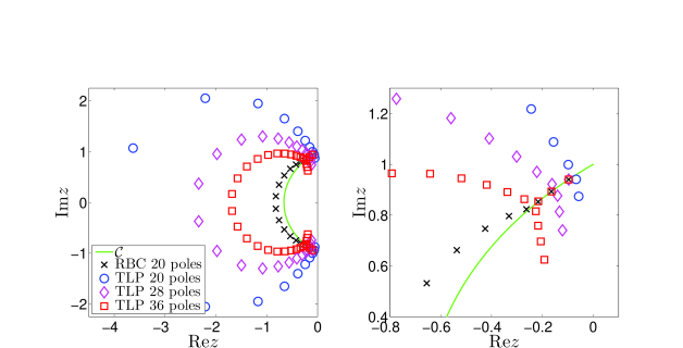
Figure 3: Scaled pole locations for compressed kernels. Here TLP means teleportation, and the curve $\mathcal{C}$ is described by the parameterization $z(\lambda)$ given in (40). In the blow-up plot there is a cross-diamond-square coalescence on $\mathcal{C}$ (near its right end). See the text for further explanation.

III.2 Blackhole perturbations

We consider the following rescaled versions of the generic master equation (1) (retaining the same stem letter $V$ for the potentials):

$$\frac{\partial^{2}\Psi_{\ell}}{\partial\tau^{2}}-\frac{\partial^{2}\Psi_{\ell}}{\partial\rho_{*}^{2}}+V^{\mathrm{RW,Z}}_{\ell}(\rho)\Psi_{\ell}=0,$$ (41)

here in terms of rescaled coordinates

$$\rho=r/(2M),\quad\tau=t/(2M),\quad\rho_{*}=\rho+\log(\rho-1).$$ (42)

Expressions for the Regge-Wheeler $V^{\mathrm{RW}}_{\ell}(\rho)$ and Zerilli $V^{\mathrm{Z}}_{\ell}(\rho)$ potentials are given in Eqs. (3) and (4) of Ref. Lau3 (expressions in terms of $r$ rather than $\rho$ are given in FHL ). The formulas we present here hold for both formalisms, and have been drawn from Refs. Lau1 ; Lau2 ; Lau3 . As before in our analysis of the flatspace radial wave equation, here we also suppress the azimuthal index $m$ on $\Psi_{\ell}$.

III.2.1 Structure of outgoing solutions

With $\sigma=2Ms$ the rescaled Laplace frequency, formal Laplace transformation of (1) yields

$$-\frac{d^{2}\widehat{\Psi}_{\ell}}{d\rho_{*}^{2}}+V^{\mathrm{RW,Z}}_{\ell}(\rho)\widehat{\Psi}_{\ell}+\sigma^{2}\widehat{\Psi}_{\ell}=0,$$ (43)

Outgoing solutions of the last equation can be expressed as an asymptotic series about $\rho=\infty$,

$$\widehat{\Psi}_{\ell}(\sigma,\rho)=a(\sigma)\sigma^{\ell}e^{-\sigma\rho_{*}}W_{\ell}(\sigma\rho,\sigma),\qquad W_{\ell}(\sigma\rho,\sigma)\mathop{\sim}_{\scriptstyle\rho\rightarrow\infty}1$$ (44)

[cf. Eq. (15) for a flatspace multipole]. Notice that $W_{\ell}(\sigma\rho,\sigma)=W_{\ell}(sr,2Ms)$, and so formally the flatspace expression $W_{\ell}(sr)=W_{\ell}(sr,0)$.

III.2.2 Radiation boundary conditions

We again assume initial data of compact support, namely that $\Psi_{\ell}(0,\rho)=0=(\partial_{\tau}\Psi_{\ell})(0,\rho)$ for $\rho>\rho_{b}-\delta$, where $\rho_{b}$ specifies the outer boundary. We now work with any $\rho\geq\rho_{b}$, in terms of which exact radiation conditions satisfied by a generic asymptotically outgoing multipole (44) have the following frequency-domain and time-domain forms Lau1 ; Lau2 ; Lau3 :

$$\sigma\widehat{\Psi}_{\ell}+\partial_{\rho_{*}}\widehat{\Psi}_{\ell}=\frac{1}{\rho}\left(1-\frac{1}{\rho}\right)\widehat{\omega}_{\ell}\widehat{\Psi}_{\ell}\iff\partial_{\tau}\Psi_{\ell}+\partial_{\rho_{*}}\Psi_{\ell}=\frac{1}{\rho}\left(1-\frac{1}{\rho}\right)\omega_{\ell}*\Psi_{\ell},$$ (45)

where the frequency domain radiation kernel is

$$\widehat{\omega}_{\ell}(\sigma,\rho)\equiv\sigma\rho\frac{W^{\prime}_{\ell}(\sigma\rho,\sigma)}{W_{\ell}(\sigma\rho,\sigma)},$$ (46)

with the prime denoting differentiation in the first argument.

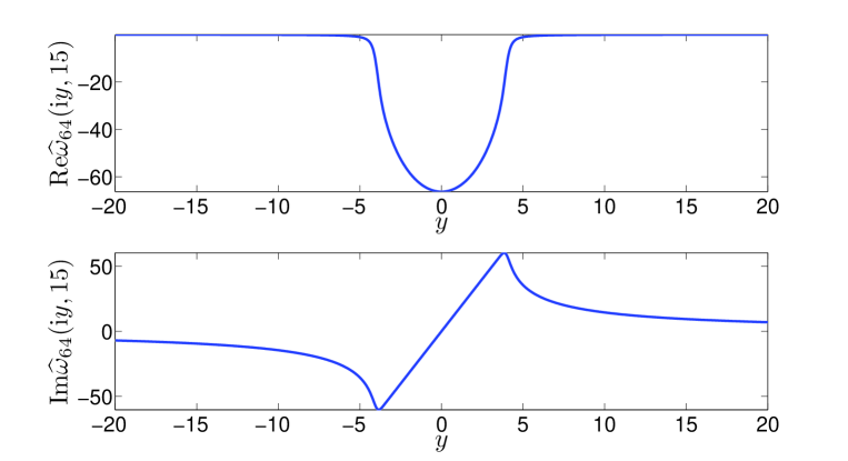
Figure 4: Profiles for an $\rho=15$, $\ell=64$ Regge-Wheeler frequency domain RBC kernel.

Refs. Lau1 ; Lau3 have argued that the kernel $\widehat{\omega}_{\ell}(\sigma,\rho)$ has the following “sum of poles” representation:

$$\widehat{\omega}_{\ell}(\sigma,\rho)=\widehat{\omega}_{\ell}^{\mathrm{pole}}(\sigma,\rho)+\widehat{\omega}_{\ell}^{\mathrm{cut}}(\sigma,\rho)\equiv\sum_{k=1}^{N_{\ell}}\frac{\sigma_{\ell,k}^{\prime}(\rho)}{\sigma-\sigma_{\ell,k}(\rho)}-\frac{1}{\pi}\int_{0}^{\infty}\frac{f_{\ell}(\chi;\rho)}{\sigma+\chi}d\chi,$$ (47)

where $f_{\ell}(\chi;\rho)\equiv\mathrm{Im}\widehat{\omega}_{\ell}(\chi e^{\mathrm{i}\pi},\rho)$ and the $\sigma_{\ell,k}(\rho)$ are simple roots of $W_{\ell}(\sigma\rho,\sigma)$ (analogous to the roots $b_{\ell,k}/r$ of $W_{\ell}(sr)$ in the flatspace case). At least for $\rho\geq 15$, the integer $N_{\ell}=\ell$ or $\ell+1$, when $\ell$ is respectively even or odd Lau1 ; Lau3 . The origin of the extra root, relative to the flatspace case, in the odd-$\ell$ case is discussed in Ref. Lau3 .

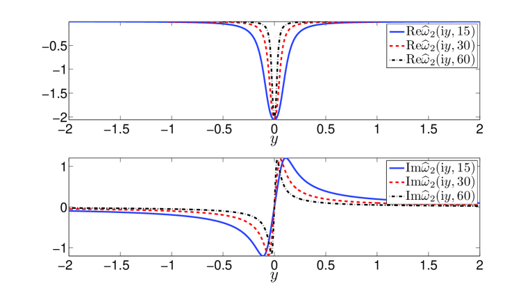
Figure 5: Profiles for $\ell=2$ Regge-Wheeler frequency domain RBC kernels. As $\rho$ increases these profiles shrink towards the origin (the same phenomena occurs for the flatspace RBC kernels).

Insofar as numerical implementation is concerned, a key requirement is the ability to evaluate the profiles $\mathrm{Re}\widehat{\omega}_{\ell}(\mathrm{i}y,\rho)$ and $\mathrm{Im}\widehat{\omega}_{\ell}(\mathrm{i}y,\rho)$ for $y\in\mathbb{R}$. These evaluations are along the imaginary $\sigma$-axis, typically the inversion contour for the inverse Laplace transform. Accurate methods for such evaluation have been described in Lau1 . In fact, these methods are not based on the sum-of-poles representation (47), but this issue is of no concern here. For example, the profiles for an $\rho=15$, $\ell=64$ Regge-Wheeler kernel are shown in Fig. 4. As $\rho$ increases these profiles “shrink” towards the origin (as do the corresponding flatspace profiles), and this phenomena is documented in Fig. 5. With the ability to numerically generate the profiles $\mathrm{Re}\widehat{\omega}_{\ell}(\mathrm{i}y,\rho)$ and $\mathrm{Im}\widehat{\omega}_{\ell}(\mathrm{i}y,\rho)$, we are then able to construct approximate kernels via Alpert-Greengard-Hagstrom (AGH) compression AGH . Here a compressed kernel is a sum of simple poles,

$$\widehat{\xi}_{\ell}(\sigma,\rho)\equiv\sum_{q=1}^{d}\frac{\gamma_{\ell,q}(\rho)}{\sigma-\beta_{\ell,q}(\rho)}\simeq\widehat{\omega}_{\ell}(\sigma,\rho),\qquad\mathrm{Re}\beta_{\ell,q}(\rho)<0,\forall q,$$ (48)

where the approximation $\widehat{\xi}_{\ell}(\sigma,\rho)$ satisfies

$$\left|\widehat{\omega}_{\ell}(\sigma,\rho)-\widehat{\xi}_{\ell}(\sigma,\rho)\right|<\varepsilon\left|\widehat{\omega}_{\ell}(\sigma,\rho)\right|,\qquad\sigma\in\mathrm{i}\mathbb{R},$$ (49)

with $\varepsilon$ a prescribed tolerance. The number $d$ clearly depends on $\varepsilon$ and $\ell$, and the numbers $\beta_{\ell,q}$ and $\gamma_{\ell,q}$ depend both on the boundary radius $\rho$ (as indicated) and on $\ell$ (the dependence on which we have restored here). The modifier compressed in the description of $\widehat{\xi}_{\ell}(\sigma,\rho)$ is apt. Indeed, as described in Sec. III.1.4, for the ordinary wave equation the exact frequency domain kernel admits a similar rational approximation with $d$ scaling as (38). Similar scaling has been observed empirically for approximations $\widehat{\xi}_{\ell}(\sigma,\rho)$ of blackhole kernels $\widehat{\omega}_{\ell}(\sigma,\rho)$ Lau1 .

Algorithm 4 summarizes our implementation of AGH compression (see Ref. Lau2 for a complete description). Let us further comment on Algorithm 4, with numbers appropriate for $\ell=2$. Typically $y_{\mathrm{max}}=300/\rho$ for step 1. For step 2 we have typically chosen 10 to 20 adaptive levels centered around the origin with 65 points at the bottom level, about $10^{3}$ grid points $y_{j}$ in all. Fig. 6 depicts an example $y$-grid. For step 3 the evaluation at each $y_{j}$ requires ODE integration in the complex plane with upwards of $10^{10}$ floating point operations in double precision (more in quad precision). Step 5 is a confirmation step meant to verify (49). Ideally, this confirmation takes place with a much larger $y$-window than $[-y_{\mathrm{max}},y_{\mathrm{max}}]$, and on a different (dense and uniform) $y$-grid. This step involves further ODE integration and is therefore as or more expensive than step 3.

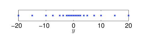
Figure 6: $y$-grid to evaluate the profiles $\mathrm{Re}\widehat{\omega}_{2}(\mathrm{i}y_{j},\rho)$ and $\mathrm{Im}\widehat{\omega}_{2}(\mathrm{i}y_{j},\rho),\forall j$. This grid has 21 points, 4 adaptive levels, and 9 points at the bottom level.

Algorithm 4 Steps for compressing an RBC kernel.

INPUT: $\ell$, $\rho=\rho_{b}$, $d$ (orbital index, dimensionless boundary radius, desired number of poles)
OUTPUT: $\{\beta_{\ell,q}(\rho),\gamma_{\ell,q}(\rho):q=1,\dots,d\}$ (compressed kernel)

1:Choose an approximation window $[-y_{\mathrm{max}},y_{\mathrm{max}}]$ on the $\sigma=\mathrm{i}y$ imaginary axis.

2:Partition $[-y_{\mathrm{max}},y_{\mathrm{max}}]$ to form a $y$-grid, typically with mesh refinement at the origin.

3:Numerically evaluate the profiles $\mathrm{Re}\widehat{\omega}_{2}(\mathrm{i}y_{j},\rho)$ and $\mathrm{Im}\widehat{\omega}_{2}(\mathrm{i}y_{j},\rho)$ on the $y$-grid.

4:Compute the numbers $\{\beta_{\ell,q}(\rho),\gamma_{\ell,q}(\rho):q=1,\dots,d\}$ by AGH compression.

5:Using $\{\beta_{\ell,q}(\rho),\gamma_{\ell,q}(\rho):q=1,\dots,d\}$, verify (49). If not verified, repeat with $d\leftarrow d+1$.

From the standpoint of implementation, the representation (48) is crucial, since it implies that the time-domain convolution can be approximately evaluated via integration of ODE at the boundary. For a typical explicit ODE scheme and a sufficiently small time-step, integration of these ODE is numerically stable since the relevant poles in (48) lie in the left-half plane. Let $\xi_{\ell}(\tau,\rho)$ be the inverse Laplace transform of $\widehat{\xi}_{\ell}(\sigma,\rho)$ with respect to $\sigma$. Then the approximate time-domain kernel $\Xi_{\ell}(t,r)\equiv(1/2M)\xi_{\ell}(t/(2M),r/(2M))$ appearing in (4) is the inverse Laplace transform (with respect to $s$) of

$$\widehat{\Xi}_{\ell}(s,r)=\sum_{q=1}^{d}\frac{\gamma_{\ell,q}(\rho)}{2M}\widehat{\Xi}_{\ell,q}(s,r),\qquad\widehat{\Xi}_{\ell,q}(s,r)=\frac{1}{s-(2M)^{-1}\beta_{\ell,q}(\rho)},$$ (50)

where, unlike in Section II, here $\ell$-dependence has not been suppressed.

III.2.3 Asymptotic waveform evaluation and teleportation

Similar to before, we introduce two kernels: (i) one $\theta_{\ell}$ for evaluation of an underlying profile, and (ii) another $\phi_{\ell}$ for AWE/teleportation of the waveform. The first type of kernel is defined by [cf. Eq. (34)]

$$\widehat{\theta}_{\ell}(\sigma,\rho)=\frac{1}{\sigma^{\ell}}\underbrace{\exp\left[\int_{\rho}^{\infty}\frac{\widehat{\omega}_{\ell}(\sigma,\eta)}{\eta}d\eta\right]}_{1/W_{\ell}(\sigma\rho,\sigma)}\,,$$ (51)

and satisfies $\widehat{\theta}_{\ell}(\sigma,\rho)\widehat{\Psi}_{\ell}(\sigma,\rho)=a(\sigma)\exp(-\sigma\rho_{*})$, as can be seen directly from Eq. (44). We can not analytically perform the integration here. However, the pole part of the kernel can be exactly integrated to remove the singularity. Indeed, we find

$$\widehat{\theta}_{\ell}(\sigma,\rho)=\frac{\exp\left[\int_{\rho}^{\infty}\frac{\widehat{\omega}_{\ell}^{\mathrm{cut}}(\sigma,\eta)}{\eta}d\eta\right]}{\sigma^{\ell}\exp\left[-\int_{\rho}^{\infty}\frac{\widehat{\omega}_{\ell}^{\mathrm{pole}}(\sigma,\eta)}{\eta}d\eta\right]}=\frac{\exp\left[\int_{\rho}^{\infty}\widehat{\omega}_{\ell}^{\mathrm{cut}}(\sigma,\eta)\eta^{-1}d\eta\right]}{\prod_{k=1}^{N_{\ell}}\big{[}\sigma-\sigma_{\ell,k}(\rho)\big{]}}.$$ (52)

Teleportation $(\rho_{1}\rightarrow\rho_{2}\leq\infty)$ is defined through the kernel [cf. Eq. (35)]

$$\widehat{\phi}_{\ell}(\sigma,\rho_{1},\rho_{2}) =-1+\underbrace{\exp\left[\int_{\rho_{1}}^{\rho_{2}}\frac{\widehat{\omega}_{\ell}(\sigma,\eta)}{\eta}d\eta\right]}_{W_{\ell}(\sigma\rho_{2},\sigma)/W_{\ell}(\sigma\rho_{1},\sigma)}.$$ (53)

Adjusting for the $(\rho^{*}_{2}-\rho^{*}_{1})$ time delay, this kernel allows for conversion of the signal at $\rho_{1}$ to the signal at $\rho_{2}$, as it satisfies

$$e^{\sigma(\rho^{*}_{2}-\rho^{*}_{1})}\widehat{\Psi}_{\ell}(\sigma,\rho_{2})=\widehat{\phi}_{\ell}(\sigma,\rho_{1},\rho_{2})\widehat{\Psi}_{\ell}(\sigma,\rho_{1})+\widehat{\Psi}_{\ell}(\sigma,\rho_{1}).$$ (54)

In the time domain we therefore recover the desired property

$$\Psi_{\ell}(\tau+(\rho^{*}_{2}-\rho^{*}_{1}),\rho_{2})=(\phi_{\ell}(\cdot,\rho_{1},\rho_{2})*\Psi_{\ell}(\cdot,\rho_{1}))(\tau)+\Psi_{\ell}(\tau,\rho_{1}).$$ (55)

Exact evaluation of the asymptotic waveform corresponds to $\rho_{2}=\infty$.

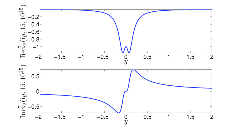
Figure 7: Teleportation kernel $\widehat{\phi}_{2}(\mathrm{i}y,15,10^{15})$ for $\rho_{1}=15\rightarrow\rho_{2}=10^{15}$.

Let us describe how we numerically approximate $\widehat{\phi}_{\ell}(\sigma,\rho_{1},\rho_{2})$ as a pole sum $\widehat{\xi}_{\ell}^{E}(\sigma,\rho_{1},\rho_{2})$. A simple version of the procedure is to follow the steps listed in Algorithm 4, replacing step 3 with evaluations of the profiles $\mathrm{Re}\widehat{\phi}_{\ell}(\mathrm{i}y_{j},\rho_{1},\rho_{2})$ and $\mathrm{Im}\widehat{\phi}_{\ell}(\mathrm{i}y_{j},\rho_{1},\rho_{2})$. To generate these profiles, we use (53), and for each $y_{j}$ evaluation point perform the $\eta$ integration using a composite Gauss-Kronrod rule. Assuming $[A,B]$ is one subinterval of $[\rho_{1},\rho_{2}]$ in the composite rule, the details are as follows. Let $\eta=AB/[(B-A)q+A]$ for $q\in[0,1]$, so that

$$\int_{A}^{B}\frac{\widehat{\omega}_{\ell}(\mathrm{i}y_{j},\eta)}{\eta}d\eta\simeq\sum_{p=1}^{N_{\mathrm{GK}}}\frac{\widehat{\omega}_{\ell}\big{(}\mathrm{i}y_{j},AB/[(B-A)q_{p}+A]\big{)}}{q_{p}+A/(B-A)}w_{p},$$ (56)

where $(q_{p},w_{p})_{p=1}^{N_{\mathrm{GK}}}$ are the 15 nodes and weights for the Gauss-Kronrod rule relative to $[0,1]$, and by the above equation we mean the same rule is separately applied to the real and imaginary parts of $\widehat{\omega}_{\ell}(\mathrm{i}y_{j},\eta)$. This numerical integration is accurate, because, in fact, for each grid-point $y_{j}$ integration of both Re$\widehat{\omega}_{\ell}(\mathrm{i}y_{j},\eta)$ and Im$\widehat{\omega}_{\ell}(\mathrm{i}y_{j},\eta)$ always involves terms of the same sign. With $N_{C}$ denoting the number composite subintervals, profiles for the RBC kernels on the $y$-grid must be computed $N_{\mathrm{GK}}\cdot N_{C}$ times. If $\rho_{2}=\infty$ the last composite interval might be handled through a semi-infinite quadrature. Approximation of $\widehat{\theta}_{\ell}(\sigma,\rho)$ follows a procedure similar (although more complicated) to the one outlined above for $\widehat{\phi}_{\ell}(\sigma,\rho_{1},\rho_{2})$.

Unfortunately, this simple procedure becomes too costly when $\rho_{2}\gg\rho_{1}$. The problem is two-fold. First, $N_{C}$ must be chosen large. Second, and more serious, the approximation window $[-y_{\mathrm{max}},y_{\mathrm{max}}]$ is fixed by the profiles for $\rho_{1}$ (the “widest” profiles in the integration). However, since, as seen from Fig. 5, the RBC profiles shrink as $\rho$ increases, the $y$-grid needs many adaptive levels to resolve the contribution to the $\eta$-integration from the profiles at and near $\rho_{2}$. The $y$-grid then must have a large number of points, on which $N_{\mathrm{GK}}\cdot N_{C}$ complex function evaluations are made (with each such evaluation costing $\simeq 10^{7}$ floating point operations). To bypass this issue, we follow another rather complicated procedure, whereby the interval $[\rho_{1},\rho_{2}]$ is first broken up into $\mathcal{N}$ chunks $[\rho_{\alpha},\rho_{\alpha+1}]$ which are typically decades like $[10^{\alpha},10^{\alpha+1}]$ if $\rho_{2}$ is very large. Each chunk has its own approximation window $[-y^{\alpha}_{\mathrm{max}},y^{\alpha}_{\mathrm{max}}]$ and (relatively small) $y^{\alpha}$-grid, and we choose these to conform with how shrunken the profiles are for $\rho\simeq\rho_{\alpha}$. Next, using the relatively simple procedure described in the last paragraph, for each of the $\mathcal{N}$ chunks we construct a compressed kernel (table) which approximates $\widehat{\phi}_{\ell}(\mathrm{i}y,\rho_{\alpha},\rho_{\alpha+1})$ as a sum of poles $\widehat{\xi}_{\ell}^{E}(\mathrm{i}y,\rho_{\alpha},\rho_{\alpha+1})$. The last step is to generate profiles (for the compression algorithm) on a large $y$-grid associated with a wide approximation window and sufficient resolution near the origin. However, these evaluations are now done via combination of all $\mathcal{N}$ tables. Therefore, they are drastically faster, since they are carried out through auxiliary evaluations made with the $\mathcal{N}$ distinct pole sums (rather than ODE integration). Finally, we note that the physical teleportation kernel used in a numerical simulation is

$$\Xi^{E}_{\ell}(t,r_{1},r_{2})=\frac{1}{2M}\xi^{E}_{\ell}(t/(2M),r_{1}/(2M),r_{2}/(2M)),\qquad$$ (57)

where $\xi_{\ell}^{E}(\tau,\rho_{1},\rho_{2})$ is the inverse Laplace transform (with respect to $\sigma$) of $\widehat{\xi}_{\ell}^{E}(\sigma,\rho_{1},\rho_{2})$.

III.2.4 Efficiency and storage

As either $\ell$ or $\varepsilon^{-1}$ becomes large the scaling observed in Lau1 for compressed, blackhole, RBC kernels appears similar to the flatspace result (38) described in Sec. III.1.4. However, we stress that these are empirical observations, and there is no corresponding proof of (38) or a similar result in the blackhole case. Nevertheless, provided that the number of approximating exponentials in the blackhole case indeed grows sublinearly with both $\ell$ and the inverse $1/\varepsilon$ of the relative approximation error [cf. Eq. (49)], our implementation of RBC satisfies the same efficient scalings (39) established for flatspace compressed kernels.

One might similarly ask whether or not our implementation of AWE for blackholes satisfies these scalings; we do not have an answer for this question, but here consider kernels from the $\ell=64$ teleportation experiment considered later in Section IV.1. Let us focus on the compressed (frequency domain) kernels $\widehat{\xi}{}_{64}(\sigma,15)$ and $\widehat{\xi}{}_{64}(\sigma,15,240)$, respectively for RBC at $\rho_{b}=15$ and teleportation from $\rho_{1}=15$ to $\rho_{2}=240$. Figure 4 has already depicted the profiles from which the 25-pole approximation $\widehat{\xi}{}_{64}(\sigma,15)$ is constructed. Notice that the approximation $\widehat{\xi}{}_{64}(\sigma,15,240)$ has 32 poles, whereas the corresponding exact flatspace teleportation kernel would have 64 poles. Similar reduction for the $\ell=64$ occurred for compressed flatspace kernels considered earlier. As depicted in Fig. 8 and similar to the situation encountered in Fig. 3, the pole locations for $\widehat{\xi}{}_{64}(\sigma,15)$ and $\widehat{\xi}{}_{64}(\sigma,15,240)$ are different. Finally, we remark that we have tried to enforce the condition that the teleportation kernel has the same pole locations as the RBC kernel [cf. the discussion around Eq. (9)]; however, we are then unable to achieve a compressed kernel with any accuracy whatsoever.

The previous paragraph has considered the large-$\ell$, small-$\varepsilon$ limits. However, in this paper we mostly consider $\varepsilon$ fixed (typically machine precision) and small $\ell$, in which case, as we have seen, $d>\ell$. We remark that this situation is similar to the case of ordinary wave propagation on $2+1$ flat spacetime. In that setting the low-$n$ (Fourier index) “circle kernels” are also expensive to evaluate, with scalings similar to (38) only exhibited in the large $n$ limit AGH .

While the previous discussion has presented scalings for various limits, in practice our implementation of RBC/teleportation for $\ell=2,3,$ and $64$ amounts to adding on the order of 20 to 30 points to the spatial domain, and modest increase in work and storage costs for the numerical experiments considered here.

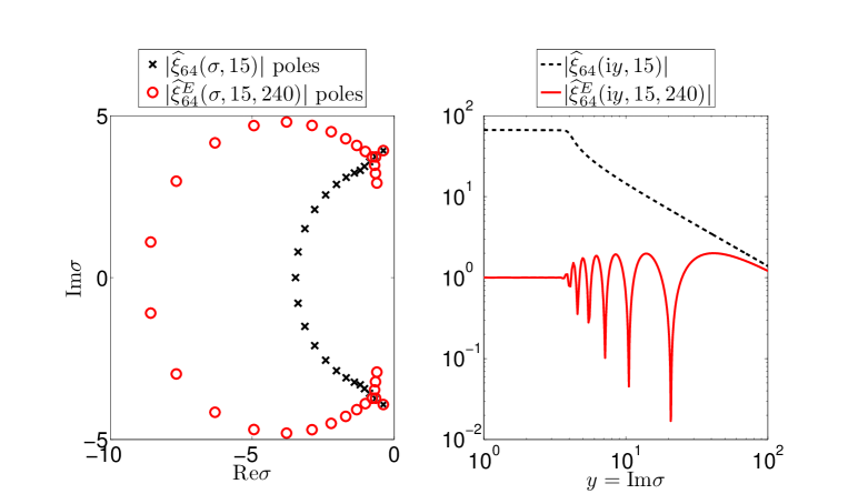
Figure 8: Compressed RBC and teleportation kernels for $\ell=64$. The right pane plots the modulus of the kernels for positive $y$. For the RBC kernel (dotted line) this corresponds to the modulus of the combined profiles shown in Fig. 4, but here with only half of the domain for the independent variable $y$.

IV Numerical Experiments

To carry out numerical simulations, we have used both the nodal Legendre discontinuous Galerkin method described in Ref. FHL (further details of this method will not be given here) and a nodal Chebyshev method. Both methods feature multiple subdomains and upwinding.

IV.1 Pulse teleportation

First consider the $\ell=2$ Regge-Wheeler equation with the same initial data (10) given in Subsection II.3. Using our multidomain nodal Chebyshev method, we perform five separate evolutions on domains with outer boundaries taken as the $b$ values corresponding to $r_{b}=30M$, $60M$, $120M$, $240M$, and $480M$. We have respectively used 32, 37, 45, 62, and 95 subintervals of uniform size, and in each case with 32 Chebyshev-Lobatto points per subinterval. Therefore, the spatial resolution for each evolution is comparable to the others. Evolutions are performed by the classical 4-stage explicit Runge Kutta method with timestep $\Delta t\simeq M(2.6794\times 10^{-4})$. For each evolution the inner boundary is $a=-200M$, and therefore the Sommerfeld boundary condition $-(\Pi+\Phi)=0$ at the inner boundary is essentially exact. For all choices of outer boundary $b$ we adopt the Laplace convolution RBC (4). Tables for $r_{b}=30M$, $60M$, $120M$, $240M$, and $480M$ respectively have 19, 19, 19, 18, and 17 poles, with each table computed in quadruple precision to satisfy the tolerance $\varepsilon=10^{-15}$. These tables are available at Kernel_web1 .

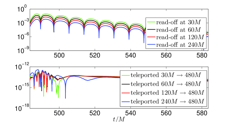
Figure 9: Errors in read-off and teleported $\ell=2$ waveforms relative to read-off waveform at $r_{2}=480M$.

In all cases the field $\Psi(t,r_{b})$ is recorded as a time series at the boundary $b$, and in all cases but the last ($b$ corresponding to $r_{b}=480M$) we “teleport” the field from $r_{1}=r_{b}$ to $r_{2}=480M$. Each approximate teleportation kernel $\Xi^{E}_{2}\simeq\Phi_{2}$ features the same pole locations as the corresponding approximate RBC kernel $\widehat{\Xi}\simeq\Omega_{2}$. For the last $r_{b}=480M$ simulation we simply record the field at the boundary, with this record then serving as a reference time series. We account for time delays by starting all recorded times series (whether read off or teleported) at time $b-6M$.

The top panel in Figure 9 plots the errors in the waveforms recorded at the different $b$ boundaries as compared to the reference $r_{b}=480M$ waveform; as expected the systematic errors are large. The bottom panel plots the errors in the ($r_{1}=r_{b}$ to $r_{2}=480M$) teleported time series relative to the reference time series. With the reference time series viewed as the “asymptotic signal”, this “AWE” clearly yields 10 or more digits of accuracy relative to simple read-off. We have found similar results using other “pulses” based on polynomial, Lorentzian, and trigonometric profiles (in all case with the initial data initially supported away from the boundary, either exactly or to machine precision).

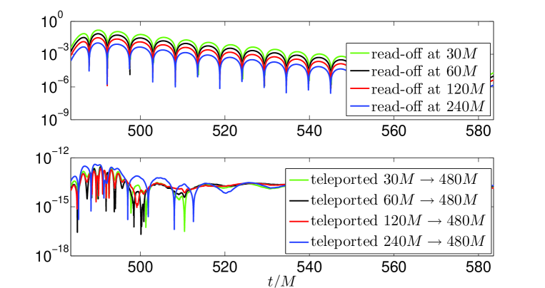
Figure 10: Errors in read-off and teleported $\ell=3$ waveforms relative to read-off waveform at $r_{2}=480M$.

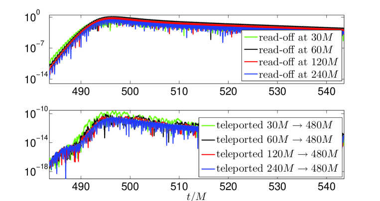
Figure 11: Errors in read-off and teleported $\ell=64$ waveforms relative to read-off waveform at $r_{2}=480M$.

We repeat the experiment for two different $\ell$ values. First, for $\ell=3$ we adopt the same initial data and experimental setup, except for the numerical tables which specify the RBC and teleportation kernels. For the $\ell=3$ experiment the number of poles for the RBC tables is either 15 or 16, and the number of poles for teleportation tables ranges from 15 to 20. The results, shown in Fig. 10, are comparable to those for $\ell=2$. Lastly, we repeat the experiment for $\ell=64$. For such a high $\ell$ the evolutions are much more expensive, due to finer oscillations in both space and time. We now use 42 points per subdomain, with the number of subdomains typically increased by a factor of 2 or 3 relative to the numbers given above for $\ell=2$. Moreover, we adopt the timestep $\Delta t=M(4.0461\times 10^{-5})$ and inner boundary $a=-80M$ which is casually disconnected from each waveform read-off/teleportation at the outer boundary. For $\ell=64$ our RBC tables have between 23 and 25 poles, and our teleportation tables between 30 and 32 poles. While these tables are large, note that even the corresponding exact flatspace RBC kernels would have 64 poles. Hence, in this experiment the savings afforded by kernel compression is already evident. Results are depicted in Fig. 11.

IV.2 Luminosities from extreme-mass-ratio binaries

An extreme mass ratio binary (EMRB) is a system comprised of a small mass-$m_{p}$ compact object (the “particle”) orbiting a much larger mass-$M$ blackhole, where the mass ratio $m_{p}/M\ll 1$. EMRB systems are expected to emit gravitational radiation in a low frequency band ($10^{-5}$ to $10^{-1}$ Hz), and therefore offer the promise of detection by a space-based gravitational wave observatory like the earlier proposed LISA project ScottHughes_LISA . Located within the solar system, such an observatory would be well approximated as positioned at $\mathscr{I}^{+}$ relative to expected sources.

A standard method for studying EMRBs uses the perturbation theory of Schwarzschild blackholes in an approximation which treats the particle as a point-like Dirac delta function. The particle follows a timelike geodesic in the background Schwarzschild spacetime and is responsible for generating small metric perturbations which radiate away (see Refs. Martel_CovariantPert ; SopuertaLaguna ; Sarbach:2001qq for modern accounts of the subject). Here we note that the axial metric perturbations for each $(\ell,m)$ mode may be combined to form a gauge invariant scalar quantity $\Psi_{\ell m}^{\mathrm{CPM}}$ which obeys Eq. (1) with the Regge-Wheeler potential $V^{\mathrm{RW}}(r)$ and a distributional forcing term $S_{\ell m}^{\mathrm{CPM}}(t,r)$. Likewise, the polar metric perturbations for each $(\ell,m)$ mode may be combined to form a gauge invariant scalar quantity $\Psi_{\ell m}^{\mathrm{Z}}$ which obeys Eq. (1) with the Zerilli potential $V^{\mathrm{Z}}(r)$ and a distributional forcing term $S_{\ell m}^{\mathrm{Z}}(t,r)$. Both $S^{\mathrm{Z}}_{\ell m}$ and $S^{\mathrm{CPM}}_{\ell m}$ are built from linear combinations of an $(\ell,m)$ mode decomposition of the stress-energy tensor and, as such, depend on the particle trajectory $(r_{p}(t),\pi/2,\phi_{p}(t))$ in the equatorial plane. Bounded and stable orbits are characterized by an eccentricity constant $e$ and a semi-latus rectum constant $p$. Upon specification of $(e,p)$, the resulting trajectory is found by integrating the relevant system of ODEs given in Eq. (5) of Ref. FHL . Appendix C of FHL gives exact expressions for $S_{\ell m}^{\mathrm{CPM,Z}}$ (see also SopuertaLaguna ; Hopper:2010uv ).

With both $S_{\ell m}^{\mathrm{CPM,Z}}$ specified, we numerically solve for $\Psi_{\ell m}^{\mathrm{CPM,Z}}$, starting with trivial initial data and smoothly turning on the source term $S_{\ell m}(t,r)$ over a timescale $\tau\simeq 150M$ to $450M$ to prohibit static Jost junk solutions which may appear in some formulations when using inconsistent initial data Field2010 ; PhysRevD.83.061503 . Respectively, Sommerfeld and Laplace convolution RBC are enforced at the left and right physical boundaries (cf. Sec. II.1). The computational domain is given by the interval $[-400M,b]$, where the tortoise coordinate value $b$ corresponds to $r_{b}=60M$ in Schwarzschild radius. Notice that as an approximation to the asymptotic signal at $\mathscr{I}^{+}$, the waveform read-off at $r_{b}$ will have an $O(r_{b}^{-1})$ systematic error, suggesting relative errors greater than one percent for $r_{b}=60M$. For our simulations, we have chosen $16$ and $3$ subdomains to the left and right of the delta function respectively and represent the numerical solution by an order-$40$ or order-$46$ polynomial on each subdomain. The distributional source terms $S_{\ell m}^{\mathrm{CPM,Z}}$ determine jump conditions in the fields $\Psi_{\ell m}^{\mathrm{CPM,Z}}$ at the particle location which we impose as junction conditions between subintervals  FHL , with the motion of the particle incorporated through a time-dependent coordinate transformation. Our particular choice of $r_{b}=60M$ ensures that the particle does not come too close to the outer computational boundary which might lead to over stretching of the coordinates. Temporal integration is carried out with a classical fourth-order Runge-Kutta method with timestep $\Delta t=M(5\times 10^{-3})$.

Computation of the luminosities for a particular orbit of the perturbing particle is a standard benchmark test. For each $(\ell,m)$ mode the energy and angular momentum luminosities at $\mathscr{I}^{+}$ (denoted by $\infty$) and at the event horizon $r=2M$ (denoted by $H$) are given by

$${\stackrel{{\scriptstyle\smash[b]{{}_{\vbox{\hbox{\large.}}}}}}{{E}}}{}^{\infty,H}_{\ell m} =\frac{1}{64\pi}\frac{\left(\ell+2\right)!}{\left(\ell-2\right)!}\left<|{\stackrel{{\scriptstyle\smash[b]{{}_{\vbox{\hbox{\large.}}}}}}{{\Psi}}}{}_{\ell m}^{\mathrm{Z}}|^{2}+|{\stackrel{{\scriptstyle\smash[b]{{}_{\vbox{\hbox{\large.}}}}}}{{\Psi}}}{}_{\ell m}^{\mathrm{CPM}}|^{2}\right>,$$ (58a)

$${\stackrel{{\scriptstyle\smash[b]{{}_{\vbox{\hbox{\large.}}}}}}{{L}}}{}^{\infty,H}_{\ell m} =\frac{\mathrm{i}m}{64\pi}\frac{\left(\ell+2\right)!}{\left(\ell-2\right)!}\left<{\stackrel{{\scriptstyle\smash[b]{{}_{\vbox{\hbox{\large.}}}}}}{{\Psi}}}{}^{\mathrm{Z}}_{\ell m}\bar{\Psi}^{\mathrm{Z}}_{\ell m}+{\stackrel{{\scriptstyle\smash[b]{{}_{\vbox{\hbox{\large.}}}}}}{{\Psi}}}{}_{\ell m}^{\mathrm{CPM}}\bar{\Psi}^{\mathrm{CPM}}_{\ell m}\right>,$$ (58b)

where the average $\left<A(t)\right>$ of a time series $A(t)$ is computed as

$$\langle A\rangle\equiv\frac{1}{T_{2}-T_{1}}\int_{T_{1}}^{T_{2}}A(t)dt,\qquad T_{2}-T_{1}=T_{r}.$$ (59)

Here $T_{r}$ is the period of radial oscillation for the particle orbit.

Before presenting our numerical results, we remark on the potential sources of error in an evaluated asymptotic waveform. At $b$ we record both $\Psi_{\ell m}^{\mathrm{CPM,Z}}(t,b)$ and their first temporal derivatives as a time-series. With the numerical setup described above, the relative pointwise error associated with these read-off waveforms is better than $10^{-10}$. An additional source of (systematic) error is due to trivial initial data which, both incorrect and inconsistent, is known to generate spurious junk. At a finite and fixed radial location, spurious junk radiation propagates away (the potential for static Jost junk is discussed in Ref. Field2010 ), although due to backscattering a “junk error tail” may develop which decays more slowly. Tail fields are expected to fall off like $t^{-4}$ at $\mathscr{I}^{+}$, and $t^{-7}$ at a fixed (much smaller) radial value. Evidently, the situation is worse at $\mathscr{I}^{+}$ where junk error tails decay more slowly. Additionally, we often need to average luminosity quantities over long periods of time. Taken together, these facts conspire to make the temporal average of a $\mathscr{I}^{+}$ waveform especially prone to contamination by junk error tails, even at late times and especially when high accuracy is desired. Unfortunately, simply waiting for junk errors to die out may not be practical, because ODE and PDE numerical integrators typically introduce numerical errors which grow linearly with time. While convolution with an approximate teleportation kernel will introduce additional error, we believe that the dominant errors in our asymptotic waveforms stem from numerical method error and spurious junk.

$m$	Alg.	${\stackrel{{\scriptstyle\smash[b]{{}_{\vbox{\hbox{\large.}}}}}}{{E}}}{}^{\infty}_{2m}$		${\stackrel{{\scriptstyle\smash[b]{{}_{\vbox{\hbox{\large.}}}}}}{{E}}}{}^{H}_{2m}$		${\stackrel{{\scriptstyle\smash[b]{{}_{\vbox{\hbox{\large.}}}}}}{{L}}}{}^{\infty}_{2m}$		${\stackrel{{\scriptstyle\smash[b]{{}_{\vbox{\hbox{\large.}}}}}}{{L}}}{}^{H}_{2m}$
0	FR	1.27486196317	$\times 10^{-8}$	1.66171571270	$\times 10^{-8}$	0		0
	AWE	1.27486196187	$\times 10^{-8}$	1.66171571269	$\times 10^{-8}$	0		0
1	FR	1.15338054092	$\times 10^{-6}$	3.08063328605	$\times 10^{-7}$	1.44066000650	$\times 10^{-5}$	2.77518962557	$\times 10^{-6}$
	AWE	1.15338054091	$\times 10^{-6}$	3.08063328606	$\times 10^{-7}$	1.44066000619	$\times 10^{-5}$	2.77518962558	$\times 10^{-6}$
2	FR	1.55967717209	$\times 10^{-4}$	1.84497995136	$\times 10^{-6}$	2.07778922470	$\times 10^{-3}$	1.85014840343	$\times 10^{-5}$
	AWE	1.55967717211	$\times 10^{-4}$	1.84497995135	$\times 10^{-6}$	2.07778922439	$\times 10^{-3}$	1.85014840342	$\times 10^{-5}$

Table 1: Mode-by-mode $\ell=2$ luminosities for the eccentric orbit described in the text. For a particle of mass $m_{p}$ these values should be scaled by $m_{p}^{2}$. The table compares our asymptotic-waveform evaluation (AWE) method with the accurate frequency domain (FR) luminosities. FR results refer to Table III of Ref. Hopper:2010uv and are quoted to a relative error of $10^{-12}$. For this experiment the outer boundary is $r_{b}=60M$.

Through $r_{b}\rightarrow r_{\infty}=2M(1\times 10^{15})$ teleportation, we approximately obtain the signals $\Psi_{\ell m}^{\mathrm{CPM,Z}}$ at $\mathscr{I}^{+}$, and with these signals compute the energy and angular momentum luminosities (58a,b). The orbital parameters $(e,p)=(0.764124,8.75455)$ and initial location $(r_{p},\phi_{p})=((pM)/(1+e\cos(\pi/2)),0)$ specify the particle’s path. As described above, we slowly turn-on the distributional source over a timescale of $\tau\simeq 150M$ to $450M$. A physically meaningful luminosity measurement will not depend on our choice of $\tau$, and from this consideration we find that by $3000M$ the spurious junk’s effect is minimal. Table 1 compares the $\ell=2$ luminosity measurements at $\mathscr{I}^{+}$ with the accurate frequency-domain results reported in Ref. Hopper:2010uv . We match their stated accuracy to better than $9$ digits.

As our final experiment we consider a circular orbit specified by the orbital parameters $(e,p)=(0,10)$. Circular-orbit luminosity measurements are time-independent, thereby allowing us to (i) better understand the influence of junk error tails on $\mathscr{I}^{+}$ waveforms and (ii) estimate errors due to our AWE procedure in a clean setting. With the same numerical parameters used for our eccentric orbit simulations, we compute $\ell=2$ luminosities at $\mathscr{I}^{+}$ and compare them to accurate frequency-domain results generated with the code described in Ref. Hopper:2010uv . By $T=6000M$ our results agree with the frequency-domain results to within a relative difference of less than $10^{-12}$. Furthermore, we find the same level of agreement when the outer boundary is moved inward to $r_{b}=30M$, in which case we use the teleportation/RBC kernel tables given in Appendix D (with the longer teleportation table for AWE).

As the final measurement time is taken earlier, the agreement becomes progressively worse due to spurious junk radiation. Indeed, the solid black line in Fig. 12 (left) plots the relative error $|{\stackrel{{\scriptstyle\smash[b]{{}_{\vbox{\hbox{\large.}}}}}}{{E}}}{}^{\infty}_{22}(t)-{\stackrel{{\scriptstyle\smash[b]{{}_{\vbox{\hbox{\large.}}}}}}{{E}}}{}^{\infty}_{22,\mathrm{FR}}|\big{/}{\stackrel{{\scriptstyle\smash[b]{{}_{\vbox{\hbox{\large.}}}}}}{{E}}}{}^{\infty}_{22,\mathrm{FR}}$ as a time-series, where ${\stackrel{{\scriptstyle\smash[b]{{}_{\vbox{\hbox{\large.}}}}}}{{E}}}{}^{\infty}_{22,\mathrm{FR}}$ is the frequency-domain value. For comparison we also compute a “luminosity” quantity ${\stackrel{{\scriptstyle\smash[b]{{}_{\vbox{\hbox{\large.}}}}}}{{E}}}{}^{b}_{22}(t)$ from ${\stackrel{{\scriptstyle\smash[b]{{}_{\vbox{\hbox{\large.}}}}}}{{\Psi}}}{}_{22}^{\mathrm{Z}}(t,b)$. The solid black line in Fig. 12 (left) shows the relative error $|{\stackrel{{\scriptstyle\smash[b]{{}_{\vbox{\hbox{\large.}}}}}}{{E}}}{}^{b}_{22}(t)-{\stackrel{{\scriptstyle\smash[b]{{}_{\vbox{\hbox{\large.}}}}}}{{E}}}{}^{b}_{22}(6500M)|\big{/}{\stackrel{{\scriptstyle\smash[b]{{}_{\vbox{\hbox{\large.}}}}}}{{E}}}{}^{b}_{22}(6500M)$, where ${\stackrel{{\scriptstyle\smash[b]{{}_{\vbox{\hbox{\large.}}}}}}{{E}}}{}^{b}_{22}(6500M)$ is a late-time computation less contaminated by spurious junk. Comparing the black and red lines, we see that the junk error tails at $\mathscr{I}^{+}$ persist longer than those at the outer boundary $b$. This observation suggests that spurious junk radiation is a stubborn problem for high accuracy studies. The right panel of Fig. 12 indicates that the energy luminosity errors (due to spurious junk) respectively decay as $t^{-8}$ and $t^{-5}$ for a fixed radial value and $\mathscr{I}^{+}$. If we view ${\stackrel{{\scriptstyle\smash[b]{{}_{\vbox{\hbox{\large.}}}}}}{{\Psi}}}{}_{\mathrm{exact}}$ as either ${\stackrel{{\scriptstyle\smash[b]{{}_{\vbox{\hbox{\large.}}}}}}{{\Psi}}}{}_{22}(6500,b)$ or ${\stackrel{{\scriptstyle\smash[b]{{}_{\vbox{\hbox{\large.}}}}}}{{\Psi}}}{}_{22}^{\infty}$, then these rates are consistent with the expected decay rate for field error tails $\Psi_{\text{junk tail}}$ and the relationship for a numerically computed energy luminosity ${\stackrel{{\scriptstyle\smash[b]{{}_{\vbox{\hbox{\large.}}}}}}{{E}}}{}\propto|{\stackrel{{\scriptstyle\smash[b]{{}_{\vbox{\hbox{\large.}}}}}}{{\Psi}}}{}_{\mathrm{exact}}+{\stackrel{{\scriptstyle\smash[b]{{}_{\vbox{\hbox{\large.}}}}}}{{\Psi}}}{}_{\text{junk tail}}|^{2}\simeq|{\stackrel{{\scriptstyle\smash[b]{{}_{\vbox{\hbox{\large.}}}}}}{{\Psi}}}{}_{\mathrm{exact}}|^{2}+2\mathrm{Re}\big{(}{\stackrel{{\scriptstyle\smash[b]{{}_{\vbox{\hbox{\large.}}}}}}{{\Psi}}}{}_{\mathrm{exact}}{\stackrel{{\scriptstyle\smash[b]{{}_{\vbox{\hbox{\large.}}}}}}{{\Psi}}}{}_{\text{junk tail}}\big{)}$.

$m$	Alg.	${\stackrel{{\scriptstyle\smash[b]{{}_{\vbox{\hbox{\large.}}}}}}{{E}}}{}^{\infty}_{2m}$		${\stackrel{{\scriptstyle\smash[b]{{}_{\vbox{\hbox{\large.}}}}}}{{E}}}{}^{H}_{2m}$		${\stackrel{{\scriptstyle\smash[b]{{}_{\vbox{\hbox{\large.}}}}}}{{L}}}{}^{\infty}_{2m}$		${\stackrel{{\scriptstyle\smash[b]{{}_{\vbox{\hbox{\large.}}}}}}{{L}}}{}^{H}_{2m}$
1	FR	1.93160935116	$\times 10^{-7}$	1.22691683145	$\times 10^{-9}$	6.10828509933	$\times 10^{-6}$	3.87985168700	$\times 10^{-8}$
	AWE	1.93160935114	$\times 10^{-7}$	1.22691683145	$\times 10^{-9}$	6.10828509953	$\times 10^{-6}$	3.87985168700	$\times 10^{-8}$
2	FR	5.36879547910	$\times 10^{-5}$	1.13082774691	$\times 10^{-8}$	1.69776220056	$\times 10^{-3}$	3.57599132155	$\times 10^{-7}$
	AWE	5.36879547910	$\times 10^{-5}$	1.13082774691	$\times 10^{-8}$	1.69776220057	$\times 10^{-3}$	3.57599132154	$\times 10^{-7}$

Table 2: Mode-by-mode $\ell=2$ luminosities for the circular orbit described in the text. For a particle of mass $m_{p}$ these values should be scaled by $m_{p}^{2}$. The table compares our asymptotic-waveform evaluation (AWE) results with frequency domain (FR) results computed by the code described in Ref. Hopper:2010uv . We are grateful to S. Hopper for generating these previously unpublished FR luminosity values.

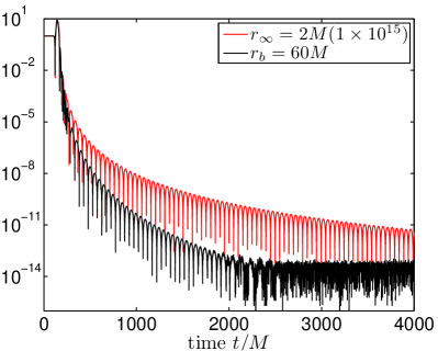
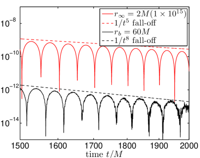
Figure 12: Energy luminosity errors due to spurious junk radiation. Both panels show $|{\stackrel{{\scriptstyle\smash[b]{{}_{\vbox{\hbox{\large.}}}}}}{{E}}}{}^{\infty}_{22}(t)-{\stackrel{{\scriptstyle\smash[b]{{}_{\vbox{\hbox{\large.}}}}}}{{E}}}{}^{\infty}_{22,\mathrm{FR}}|/{\stackrel{{\scriptstyle\smash[b]{{}_{\vbox{\hbox{\large.}}}}}}{{E}}}{}^{\infty}_{22,\mathrm{FR}}$ (red line, $r_{\infty}$) and $|{\stackrel{{\scriptstyle\smash[b]{{}_{\vbox{\hbox{\large.}}}}}}{{E}}}{}^{b}_{22}(t)-{\stackrel{{\scriptstyle\smash[b]{{}_{\vbox{\hbox{\large.}}}}}}{{E}}}{}^{b}_{22}(6500M)|/{\stackrel{{\scriptstyle\smash[b]{{}_{\vbox{\hbox{\large.}}}}}}{{E}}}{}^{b}_{22}(6500M)$ (black line, $r_{b}$) as a time-series. Comparing the black and red lines, we see that the energy luminosity error (due to spurious junk) is particularly persistent at $\mathscr{I}^{+}$. See the text for further explanation.

V Conclusions

In the context of the Regge-Wheeler/Zerilli (describing blackhole perturbations) and ordinary (describing acoustic phenomena) wave equations we have developed a procedure for obtaining the asymptotic far-field signal from a time-series recorded at a finite radial value located beyond the spatial compact support of the initial data. Furthermore, we have viewed asymptotic waveform evaluation as a limiting case of signal teleportation between two finite radial values. For each of these wave equations our steps are to (i) write down the exact relationship for teleportation in the Laplace frequency domain, (ii) approximate this relationship along the inversion contour (of the inverse Laplace transform) by a sum of simple poles, and (iii) then represent, through inversion, the asymptotic signal as a convolution [cf. Eq. (8)] of the solution with time-domain kernel [cf. Eq. (7)] comprised of damped exponentials. A similar recipe might be used both to impose boundary conditions for and evaluate asymptotic waveforms from perturbations of a Kerr blackhole. The Teukolsky equation describing such perturbations is, like the cases treated in this paper, separable in the frequency domain.

Through pre-computed numerical tables specifying each exponential’s strength and damping rate, we have demonstrated that accurate asymptotic waveform evaluation through teleportation can be easily implemented. Our simulations based on these numerical tables correctly exhibit $t^{-4}$ as the asymptotic decay rate for $\ell=2$ tails. We have also performed generic-orbit, extreme-mass-ratio, binary simulations. From the solution recorded as close as $30M$ and $60M$, we compute far-field luminosities which agree with accurate frequency domain results to a relative error of better than $10^{-9}$ ($10^{-12}$ for circular orbits). Our studies indicate that spurious junk radiation is particularly problematic for $\mathscr{I}^{+}$ computations, because far-field luminosity errors (due to spurious junk) decay at a slow rate. These results have been achieved without a compactification scheme to include $\mathscr{I}^{+}$ in the computational domain. Instead, they have relied on a Laplace convolution (8) which, decoupled from a numerical evolution, can also be carried out as a post-processing step on an existing time series. Finally, we have demonstrated effective signal teleportation between two finite radial locations, for $\ell=2,3,64$ and with relative errors $\simeq 10^{-10}$. These demonstrations are a powerful test of our AWE/teleportation method’s accuracy as well as a practical sanity check of its implementation.

As discussed in Sec. III.2.4, our Laplace-convolution RBC and AWE methods would seem efficient from work and storage standpoints. Lower $\ell$ kernels appear similar to the case of ordinary wave propagation on $2+1$ flat spacetime. In that setting the low-$n$ (Fourier index) “circle kernels” are also expensive to evaluate to account for tail-like phenomena. In any case, for the $\ell=2,3,64$ cases considered in this paper a kernel’s overall computational cost is roughly equivalent to to adding 20 to 30 points to the spatial domain. Moreover, it is non-intrusive, requiring no grid stretching or supplemental coordinate transformations, and may be carried out at any radial value beyond the spatial compact support of the initial data and sources. Finally, in their frequency-domain form, our kernels might be used to implement radiation boundary conditions and AWE in frequency-domain codes. Here we envision that the kernels would first undergo a “Wick rotation” prior to use.

While the results of this paper are encouraging, we believe that further careful study is merited. First, the task of computing teleportation/AWE tables is daunting for a number of reasons. The main one is cost. Here we refer to the offline cost in generating a table, not the cost incurred by the user implementing AWE with such a table. As discussed in Sec. III.2.3, generation of AWE kernels costs upwards of $10^{13}$ floating point operations. Moreover, since the cost is offline, with the resulting numerical table then “good for all time”, we believe the process should be carried out in quadruple precision in order to achieve $\varepsilon=10^{-15}$ error tolerances. This further adds to the cost. Due to the difficulties associated with the computation of AWE tables, we have not adequately isolated all sources of error in their construction. A systematic and optimized procedure for computing kernels would greatly reduce the offline costs. One possibility is an application specific quadrature rule. So far, we have employed the familiar Gauss-Kronrod rule, which is designed for high-order integration of polynomials. We might instead design a quadrature rule which is exact for the corresponding flatspace kernels Antil:ROQ .

We plan to construct a family of RBC and AWE tables for general use: Regge-Wheeler and Zerilli tables likely for $2\leq\ell\leq 64$, boundary radii $\rho_{b}=15,30,60,120$, and an evaluation radius $\rho_{\infty}=1\times 10^{15}$ (or $\rho_{\infty}=\infty$ with a semi-infinite quadrature rule, see Sec. III.2.3). All kernels used in this paper, as well as these others, will be available at Kernel_web1 .

VI Acknowledgements

This work has been substantially supported by NSF grant No. PHY 0855678 to the University of New Mexico; AGB and SRL gratefully acknowledge this support. AGB’s contributions to this work were also supported by NSF Grant No. 0739417 as an Undergraduate Research Project supervised by SRL. SEF acknowledges support from the Joint Space Science Institute, NSF Grants No. PHY 1208861 and No. PHY 1005632 to the University of Maryland, and NSF grant No. PHY05-51164 to the University of California at Santa Barbara. SRL is also grateful for support from the Erwin Schrödinger Institute for Mathematical Physics, Vienna, during the workshop Dynamics of General Relativity Analytical and Numerical Approaches, 4 July to 2 September, 2011. SEF thanks the Kavli Institute for Theoretical Physics, University of California at Santa Barbara, where this work was completed, for its hospitality. We are grateful for comments from M. Blair, P. Cañizares, M. Cao, C. Evans, T. Hagstrom, S. Hopper, L. Lehner, M. Tiglio, B. Whiting, and A. Zenginoğlu. We further thank A. Zenginoğlu for comments on the manuscript, and SRL particularly thanks C. Evans for discussions early on in the development of RBCs which also influenced the ideas presented here.

Appendix A Error estimates

Suppose that we have an “exact” kernel $B(t)$ and an associated Laplace convolution

$$(B*\Psi)(t)=\int_{0}^{t}B(t-t^{\prime})\Psi(t^{\prime})dt^{\prime}.$$ (60)

We then have the following result for the relative convolution error associated with using an approximate kernel $A(t)$ in place of $B(t)$:

$$\|A*\Psi-B*\Psi\|_{L_{2}(0,\infty)}\leq\sup_{s\in\mathrm{i}\mathbb{R}}\frac{|\widehat{A}(s)-\widehat{B}(s)|}{|\widehat{B}(s)|}\|B*\Psi\|_{L_{2}(0,\infty)},$$ (61)

provided that $\widehat{B}(s)\neq 0$ holds for all $s\in\mathrm{i}\mathbb{R}$. If this condition fails, we have instead

$$\|A*\Psi-B*\Psi\|_{L_{2}(0,\infty)}\leq(2\pi)^{-1/2}\sup_{s\in\mathrm{i}\mathbb{R}}|\widehat{A}(s)-\widehat{B}(s)|\cdot\|\Psi\|_{L_{2}(0,\infty)},$$ (62)

Before discussing their consequences, let us verify (61) and (62).

A Laplace convolution may be viewed as a Fourier convolution, that is

$$\int_{0}^{t}B(t-t^{\prime})\Psi(t^{\prime})dt^{\prime}=\int_{-\infty}^{\infty}B(t-t^{\prime})\Psi(t^{\prime})dt^{\prime},$$ (63)

if we adopt that viewpoint that $B(t)$ and $\Psi(t)$ are causal functions, i.e. $B(t)=B(t)\theta(t)$ and $\Psi(t)=\Psi(t)\theta(t)$, where $\theta(t)$ is the Heaviside step function. With this viewpoint, the Fourier transform of $\Psi(t)$, for example, is

$$\widetilde{\Psi}(\omega)=\frac{1}{\sqrt{2\pi}}\int_{0}^{\infty}\exp(-\mathrm{i}\omega t)\Psi(t)dt,$$ (64)

with the following formal relationship holding between the Fourier and Laplace transforms:

$$\widetilde{\Psi}(\omega)=\frac{1}{\sqrt{2\pi}}\widehat{\Psi}(\mathrm{i}\omega).$$ (65)

To establish (61), we view $A*\Psi$ and $B*\Psi$ as Fourier convolutions of casual functions (each convolution is again a causal function), and with the Parseval and Fourier convolution theorems find that

$$\begin{split}\|A*\Psi-B*\Psi\|_{L_{2}(0,\infty)}&=\|A*\Psi-B*\Psi\|_{L_{2}(\mathbb{R})}\\ &=\|\widetilde{A}\widetilde{\Psi}-\widetilde{B}\widetilde{\Psi}\|_{L_{2}(\mathbb{R})}\\ &\leq\sup_{\omega\in\mathbb{R}}\left|\frac{\widetilde{A}(\omega)-\widetilde{B}(\omega)}{\widetilde{B}(\omega)}\right|\|\widetilde{B}\widetilde{\Psi}\|_{L_{2}(\mathbb{R})}\\ &=\sup_{s\in\mathrm{i}\mathbb{R}}\left|\frac{\widehat{A}(s)-\widehat{B}(s)}{\widehat{B}(s)}\right|\|\widetilde{B}\widetilde{\Psi}\|_{L_{2}(\mathbb{R})}.\end{split}$$ (66)

Using the inverse Fourier transform on the final term to work backwards (again with the Parseval and Fourier convolution theorems), we obtain (61). The alternative estimate (62) follows by nearly the same calculation.

We view (61) as an estimate for either of the error quantities

$$\mathcal{E}_{1} \equiv\big{\|}\Omega_{\ell}(\cdot,r_{b})*\Psi_{\ell}(\cdot,r_{b})-\Xi_{\ell}(\cdot,r_{b})*\Psi_{\ell}(\cdot,r_{b})\|_{L_{2}(0,\infty)}$$ (67a)

$$\mathcal{E}_{2} \equiv\big{\|}\Phi_{\ell}(\cdot,r_{b},r_{\infty})*\Psi_{\ell}(\cdot,r_{b})-\Xi^{E}_{\ell}(\cdot,r_{b},r_{\infty})*\Psi_{\ell}(\cdot,r_{b})\|_{L_{2}(0,\infty)},$$ (67b)

and (62) as an estimate for

$$\mathcal{E}_{3} \equiv\big{\|}\Phi_{\ell}(\cdot,r_{b},r_{\infty})*\Psi_{\ell}(\cdot,r_{b})-\Phi_{\ell}(\cdot,r_{b},\infty)*\Psi_{\ell}(\cdot,r_{b})\|_{L_{2}(0,\infty)}.$$ (68)

Quantities (67a,b) measure the quality of our numerical approximations for RBC and teleportation kernels, while (68) measures the quality of using the exact waveform at a large (but finite) radius $r_{\infty}\neq\infty$ as an approximation for the asymptotic waveform at $\mathscr{I}^{+}$. We only present details for (67a) and (68).

To use the estimate (61) for (67a), let $B(t)=\Omega_{\ell}(t,r_{b})$ and $A(t)=\Xi_{\ell}(t,r_{b})$. Using Algorithm 4 we approximate $\widehat{B}(\mathrm{i}y)=\widehat{\Omega}_{\ell}(\mathrm{i}y,r)$ along the axis of imaginary Laplace frequency, demanding that

$$\sup_{y\in\mathbb{R}}\frac{|\widehat{\Omega}_{\ell}(\mathrm{i}y,r)-\widehat{\Xi}_{\ell}(\mathrm{i}y,r)|}{|\widehat{\Omega}_{\ell}(\mathrm{i}y,r)|}<\varepsilon.$$ (69)

Here $\widehat{\Xi}_{\ell}(\mathrm{i}y,r)=\widehat{A}(\mathrm{i}y)$ is a sum of simple poles specified by one of our numerical tables, and $\varepsilon$ is the desired tolerance. This formula is essentially (49) written earlier in dimensionless variables for the blackhole case. With the above identifications, Eqs. (69) and (61) yield

$$\mathcal{E}_{1}<\varepsilon\big{\|}\Omega_{\ell}(\cdot,r_{b})*\Psi_{\ell}(\cdot,r_{b})\|_{L_{2}(0,\infty)}.$$ (70)

Note that (69) is an a posteriori bound; it is verified in step 5 of Algorithm 4.

To facilitate the analysis for (68), we use $r_{1}$ and $r_{2}$ in place of $r_{b}$ and $r_{\infty}$, with $B(t)=\Phi_{\ell}(t,r_{1},\infty)$ and $A(t)=\Phi_{\ell}(t,r_{1},r_{2})$. Now referring to the absolute estimate (62), we must control the factor

$$\big{|}\widehat{A}(s)-\widehat{B}(s)\big{|}=\left|\frac{W(sr_{2},2Ms)}{W(sr_{1},2Ms)}-\frac{1}{W(sr_{1},2Ms)}\right|,$$ (71)

here expressed for the blackhole case [cf. Eq. (53)]. Further analysis of the blackhole case would presumably rely on the known asymptotic expansions (see footnote 4) for $W(sr,2Ms)=W(\sigma\rho,\sigma)$, but would seem difficult. Therefore, to proceed, we switch to the simpler flatspace case by setting $M=0$ and using the formal result $W(sr,0)=W(sr)$. The expression (15) for $W_{\ell}(sr)$ then gives

$$\big{|}\widehat{A}(s)-\widehat{B}(s)\big{|}=\left|\frac{\sum_{k=1}^{\ell}c_{\ell k}(sr_{2})^{-k}}{\sum_{j=0}^{\ell}c_{\ell j}(sr_{1})^{-j}}\right|=\left(\frac{r_{1}}{r_{2}}\right)^{\ell}\left|\frac{\sum_{k=1}^{\ell}c_{\ell k}(sr_{2})^{\ell-k}}{\sum_{j=0}^{\ell}c_{\ell j}(sr_{1})^{\ell-j}}\right|.$$ (72)

We now show that

$$\sup_{s\in\mathrm{i}\mathbb{R}}\left(\frac{r_{1}}{r_{2}}\right)^{\ell}\left|\frac{\sum_{k=1}^{\ell}c_{\ell k}(sr_{2})^{\ell-k}}{\sum_{j=0}^{\ell}c_{\ell j}(sr_{1})^{\ell-j}}\right|=O(1/r_{2}).$$ (73)

To establish this claim, note that the denominator of the expression inside the operation of complex modulus is the Bessel polynomial with zeros $b_{\ell,k}$. Therefore, we expand the expression as a sum of simple poles, thereby finding

$$\sup_{s\in\mathrm{i}\mathbb{R}}\left(\frac{r_{1}}{r_{2}}\right)^{\ell}\left|\frac{\sum_{k=1}^{\ell}c_{\ell k}(sr_{2})^{\ell-k}}{\sum_{j=0}^{\ell}c_{\ell j}(sr_{1})^{\ell-j}}\right|\leq\sup_{s\in\mathrm{i}\mathbb{R}}\sum_{j=1}^{\ell}\left|\frac{\mu_{j}(r_{1},r_{2})}{sr_{1}-b_{\ell,j}}\right|\leq\sum_{j=1}^{\ell}\left|\frac{\mu_{j}(r_{1},r_{2})}{\mathrm{Re}b_{\ell,j}}\right|.$$ (74)

The residue formula for a simple pole shows that each coefficient in the expansion obeys $\mu_{j}(r_{1},r_{2})=O(1/r_{2})$, establishing the claim. These calculations show that (returning to $r_{b}$ and $r_{\infty}$ for $r_{1}$ and $r_{2}$)

$$\mathcal{E}_{3}=O(1/r_{\infty})\|\Psi_{\ell}(\cdot,r_{b})\big{\|}_{L_{2}(0,\infty)}.$$ (75)

While we have not proved a similar formula for the blackhole case, this formula (an a priori estimate) has motivated our choice $r_{\infty}=2M(1\times 10^{15})$ for double precision arithmetic.

Appendix B Derivation of NRBC without Laplace transform

This appendix derives the nonlocal nonreflecting boundary condition (24) without appealing to the Laplace transform. In order to elucidate the main ideas, we choose to focus on the representative $\ell=2$ case; the derivation for generic $\ell$ is more cumbersome but similar. The Sommerfeld residual for the solution (13) is

$$\partial_{t}\Psi_{2}+\partial_{r}\Psi_{2}=-\frac{3}{r^{2}}f^{(1)}(t-r)-\frac{6}{r^{3}}f(t-r),$$ (76)

and we will show that this equation can be expressed as

$$\partial_{t}\Psi_{2}+\partial_{r}\Psi_{2}=\frac{1}{r}\int_{0}^{t}\Omega_{2}(t-t^{\prime},r)\Psi_{2}(t^{\prime},r)dt^{\prime}$$ (77)

$$-\exp\Big{(}-\frac{3t}{2r}\Big{)}\Big{\{}\sin\Big{(}\frac{\sqrt{3}t}{2r}\Big{)}\Big{[}\frac{\sqrt{3}}{r^{2}}f^{(1)}(-r)\Big{]}+\cos\Big{(}\frac{\sqrt{3}t}{2r}\Big{)}\Big{[}\frac{3}{r^{2}}f^{(1)}(-r)+\frac{6}{r^{3}}f(-r)\Big{]}\Big{\}},$$

where the $\ell=2$ time-domain kernel is [cf. (23)]

$$\Omega_{2}(t,r)=\frac{z_{+}}{r}\exp\left(\frac{z_{+}}{r}t\right)+\frac{z_{-}}{r}\exp\left(\frac{z_{-}}{r}t\right),\quad z_{\pm}=-\frac{3}{2}\pm\mathrm{i}\frac{\sqrt{3}}{2}.$$ (78)

Let us postpone establishing (77), and first consider its consequences. If we assume (14) and evaluate (77) at $r=r_{b}$, then the last two terms on the righthand side vanish and we have the desired result

$$\big{[}\partial_{t}\Psi_{2}(t,r)+\partial_{r}\Psi_{2}(t,r)\big{]}\big{|}_{r=r_{b}}=\frac{1}{r_{b}}\big{[}\Omega_{2}(\cdot,r_{b})*\Psi_{2}(\cdot,r_{b})\big{]}(t).$$ (79)

Indeed, from (i) the identity

$$f(t-r)=\frac{1}{6}r^{2}(\partial_{t}+\partial_{r})r^{2}(\partial_{t}+\partial_{r})\Psi_{2}(t,r)$$ (80)

and the assumptions that (ii) $\Psi_{2}(0,r)=0=(\partial_{t}\Psi_{2})(0,r)$ in a neighborhood of $r_{b}$ and (iii) $\Psi_{2}$ obeys the radial wave equation, we conclude that $f^{(1)}(-r_{b})=0=f(-r_{b})$. Therefore, as claimed, the $\ell=2$ case of (24) holds exactly subject to our assumption (14) on the initial data. Note that, even if (14) does not hold, the last term in (77) decays exponentially.

Now let us verify (77), assuming only the outgoing solution (13) without any restriction on the initial data. That is, we only assume that $\Psi_{2}=\Psi_{2}^{(1)}$, with no contribution from $\Psi_{2}^{(-1)}$ [cf. (11)]. First consider the quadratic polynomial

$$p(z)\equiv\sqrt{\frac{2z}{\pi}}z^{2}e^{z}K_{5/2}(z)=z^{2}+3z+3,\qquad p(z_{\pm})=0,$$ (81)

where $K_{\nu}(z)$ is the MacDonald function (cf. footnote 2). We appeal to the form (13) of $\Psi_{2}$, and via integration by parts shift all time derivatives off of $f$ and onto the exponentials. For generic $z$ (either $z_{+}$ or $z_{-}$) the calculation gives

$$\begin{split}\frac{z}{r^{2}}\int_{0}^{t}\exp\left[\frac{z}{r}(t-t^{\prime})\right]&\left[f^{(2)}(t^{\prime}-r)+\frac{3}{r}f^{(1)}(t^{\prime}-r)+\frac{3}{r^{2}}f(t^{\prime}-r)\right]\mathrm{d}t^{\prime}\\ &=\frac{z}{r^{2}}f^{(1)}(t-r)+\frac{1}{r^{3}}\big{(}z^{2}+3z\big{)}f(t-r)\\ &-\exp\left(\frac{z}{r}t\right)\left[\frac{z}{r^{2}}f^{(1)}(-r)+\frac{1}{r^{3}}\big{(}z^{2}+3z\big{)}f(-r)\right]\\ &+(z^{2}+3z+3)\frac{z}{r^{4}}\int_{0}^{t}\exp\left[\frac{z}{r}(t-t^{\prime})\right]f(t^{\prime}-r)\mathrm{d}t^{\prime}.\end{split}$$ (82)

Since $z$ is either $z_{+}$ or $z_{-}$, the prefactor in the last term is $p(z_{\pm})=0$. Therefore,

$$\begin{split}\frac{z_{+}}{r^{2}}\int_{0}^{t}\exp&\left[\frac{z_{+}}{r}(t-t^{\prime})\right]\Psi_{2}(t^{\prime},r)\mathrm{d}t^{\prime}+\frac{z_{-}}{r^{2}}\int_{0}^{t}\exp\left[\frac{z_{-}}{r}(t-t^{\prime})\right]\Psi_{2}(t^{\prime},r)\mathrm{d}t^{\prime}\\ &=\frac{1}{r^{2}}(z_{+}+z_{-})f^{(1)}(t-r)+\frac{1}{r^{3}}(z_{+}^{2}+3z_{+}+z_{-}^{2}+3z_{-})f(t-r)\\ &-\exp\left(\frac{z_{+}}{r}t\right)\left[\frac{z_{+}}{r^{2}}f^{(1)}(-r)+\frac{1}{r^{3}}\big{(}z_{+}^{2}+3z_{+}\big{)}f(-r)\right]\\ &-\exp\left(\frac{z_{-}}{r}t\right)\left[\frac{z_{-}}{r^{2}}f^{(1)}(-r)+\frac{1}{r^{3}}\big{(}z_{-}^{2}+3z_{-}\big{)}f(-r)\right].\end{split}$$ (83)

Combination of the last result with $z_{\pm}=-\frac{1}{2}(3\mp\mathrm{i}\sqrt{3})$ then gives

$$\frac{1}{r}\int_{0}^{t}\Omega_{2}(t-t^{\prime},r)\Psi_{2}(t^{\prime},r)dt^{\prime}=-\frac{3}{r^{2}}f^{(1)}(t-r)-\frac{6}{r^{3}}f(t-r)$$ (84)

$$+\exp\Big{(}-\frac{3t}{2r}\Big{)}\Big{\{}\sin\Big{(}\frac{\sqrt{3}t}{2r}\Big{)}\Big{[}\frac{\sqrt{3}}{r^{2}}f^{(1)}(-r)\Big{]}+\cos\Big{(}\frac{\sqrt{3}t}{2r}\Big{)}\Big{[}\frac{3}{r^{2}}f^{(1)}(-r)+\frac{6}{r^{3}}f(-r)\Big{]}\Big{\}},$$

from which we immediately get (77).

Appendix C RBC for other foliations of Schwarzschild

In terms of the standard time slices and area radius the Schwarzschild line-element is

$$ds^{2}=-fdt^{2}+f^{-1}dr^{2}+r^{2}d\theta^{2}+\sin^{2}\theta d\phi^{2},\qquad f\equiv 1-2M/r.$$ (85)

Define the outgoing (future and outward pointing) null vector

$$z^{+}\equiv\frac{1}{f^{1/2}}\frac{\partial}{\partial t}+f^{1/2}\frac{\partial}{\partial r}\implies f^{1/2}z^{+}=\frac{\partial}{\partial t}+\frac{\partial}{\partial x},$$ (86)

again where $x=r_{*}$ is the tortoise coordinate. The exact RBC for these coordinates is essentially (45), with appropriate rescalings by $2M$ factors. In particular, with $\Omega_{\ell}(t,r)=(2M)^{-1}\omega_{\ell}(t/(2M),r/(2M))$, we write the RBC as

$$f^{1/2}z^{+}[\Psi]=r^{-1}f(\Omega_{\ell}*\Psi),$$ (87)

where $f^{1/2}z^{+}[\Psi]=X$ from (2). To implement the boundary condition, we approximate it through the replacement $\Omega_{\ell}\rightarrow\Xi_{\ell}$.

Following Zenginoğlu’s Zenginoglu:2009ey analysis, we now consider a change of time slices defined by the new time variable

$$\lambda=t-h(r),$$ (88)

where $h(r)$ is the height function. In terms of $\lambda$ the line-element becomes

$$ds^{2}=-N^{2}d\lambda^{2}+g_{rr}(dr+V^{r}d\lambda)(dr+V^{r}d\lambda)+r^{2}d\theta^{2}+\sin^{2}\theta d\phi^{2},$$ (89)

where the lapse, radial lapse, and radial component of the shift vector are respectively

$$N^{2}=\frac{f}{1-(fH)^{2}},\qquad\sqrt{g_{rr}}=\frac{1}{N},\qquad V^{r}=-fHN^{2}.$$ (90)

Here $H=dh/dr$ is the derivative of the height function. Define the outgoing ($+$) and incoming ($-$) null vectors

$$w^{\pm}\equiv\frac{1}{N}\frac{\partial}{\partial\lambda}-\left(\frac{V^{r}}{N}\mp\frac{1}{\sqrt{g_{rr}}}\right)\frac{\partial}{\partial r}.$$ (91)

Then $z^{+}=\exp(\vartheta)w^{+}$ and $w^{+}=\exp(-\vartheta)z^{+}$, where the boost angle is

$$\vartheta=\frac{1}{2}\log\left[\frac{1+\sqrt{g_{rr}}N^{-1}V^{r}}{1-\sqrt{g_{rr}}N^{-1}V^{r}}\right]=\frac{1}{2}\log\left[\frac{1-NfH\sqrt{1-(fH)^{2}}}{1+NfH\sqrt{1-(fH)^{2}}}\right].$$ (92)

Therefore, with respect to the new slices the exact RBC is

$$w^{+}[\Psi]=r^{-1}e^{-\vartheta}f^{1/2}(\Omega_{\ell}*\Psi),$$ (93)

and it can similarly be approximated through the replacement $\Omega_{\ell}\rightarrow\Xi_{\ell}$. As given by Zenginoğlu Zenginoglu:2009ey , the $H$ functions for ingoing Eddington-Finkelstein and constant mean curvature foliations are respectively

$$H_{\mathrm{iEF}}=-\frac{2M}{r-2M},\qquad H_{\mathrm{CMC}}=\frac{J}{f\sqrt{J^{2}+f}},$$ (94)

where $J\equiv\frac{1}{3}Kr-Cr^{-2}$ in terms of the trace $K$ of the extrinsic curvature tensor (based on Wald’s definition Wald of the tensor) and constant $C$ of integration.

Appendix D Numerical Tables

This appendix collects the tables used for the numerical simulation documented in Subsection II.3. Table 3 determines the kernel $\Xi_{2}(t,30M)$ which approximates the exact kernel $\Omega_{2}(t,30M)=(2M)^{-1}\omega_{2}(t/(2M),15)$. The 19 locations $\beta_{2,q}$ and strengths $\gamma_{2,q}$ which make up this table have been computed in quadruple precision and satisfy the tolerance Lau3 $\varepsilon=10^{-15}$. Entries of 0.00e+00 correspond to outputs from the Alpert-Greengard-Hagstrom compression algorithm which are typically in the range $10^{-70}$ to $10^{-100}$.

We provide two different approximations for the time-domain teleportation kernel $\Phi_{2}(t,30M,2M(1\times 10^{15}))=(2M)^{-1}\phi_{2}(t/(2M),15,1\times 10^{15})$, each denoted $\Xi^{E}_{2}(t,30M,2M(1\times 10^{15}))$. Table 4 determines the first $\Xi^{E}_{2}(t,30M,2M(1\times 10^{15}))$. For this table notice that the 19 locations $\beta^{E}_{2,q}$ exactly match the $\beta_{2,q}$ listed in Table 3. Therefore, with this table the teleportation can be performed without evolving supplemental convolutions. However, we believe the tolerance for this table is only $\varepsilon=5\times 10^{-9}$. Table 5 determines the second $\Xi^{E}_{2}(t,30M,2M(1\times 10^{15}))$ which now has 26 locations $\beta^{E}_{2,q}$ and strengths $\gamma^{E}_{2,q}$. Use of this table for teleportation with the RBC specified by Table 3 requires the evolution of 26 extra convolutions. However, we believe that this second approximate kernel satisfies a tolerance of $\varepsilon=2\times 10^{-14}$.

      Regge-Wheeler RBC table for ell = 2 and rho = 15.0   Gamma strengths                                  Beta locations  -2.6076002831928367e-08 +0.00e+00                -5.4146529341487581e-01 +0.00e+00  -1.7937477396220654e-06 +0.00e+00                -4.1310954989396476e-01 +0.00e+00  -3.2816441859083765e-05 +0.00e+00                -3.1911338482076557e-01 +0.00e+00  -2.8179763264971427e-04 +0.00e+00                -2.4711219871899659e-01 +0.00e+00  -1.4509759948015657e-03 +0.00e+00                -1.9108163722923471e-01 +0.00e+00  -4.4918693070976545e-03 +0.00e+00                -1.4749601558718450e-01 +0.00e+00  -5.6790046261682662e-03 +0.00e+00                -1.1366299945908588e-01 +0.00e+00  -2.0012016782502274e-03 +0.00e+00                -8.6476935381164341e-02 +0.00e+00  -2.9649254206011509e-04 +0.00e+00                -6.4512065175451036e-02 +0.00e+00  -3.2913867328382246e-05 +0.00e+00                -4.7332374442044557e-02 +0.00e+00  -3.2675049152330702e-06 +0.00e+00                -3.4115775484663602e-02 +0.00e+00  -2.8887585153331239e-07 +0.00e+00                -2.4048935704759654e-02 +0.00e+00  -2.1640495893086479e-08 +0.00e+00                -1.6468632919283480e-02 +0.00e+00  -1.2772861871474360e-09 +0.00e+00                -1.0845690423058696e-02 +0.00e+00  -5.3164468909323526e-11 +0.00e+00                -6.7552918597864947e-03 +0.00e+00  -1.2736896522814067e-12 +0.00e+00                -3.8525630196891325e-03 +0.00e+00  -1.0598024220301938e-14 +0.00e+00                -1.8481215040788866e-03 +0.00e+00  -8.9530431033189126e-02 +6.2063746326002998e-02  -9.4779490815239023e-02 +5.9927979877488720e-02  -8.9530431033189126e-02 -6.2063746326002998e-02  -9.4779490815239023e-02 -5.9927979877488720e-02     

Table 3: Radiation boundary conditions. As indicated this table corresponds the $r_{b}=30M$ and $\ell=2$.

      Regge-Wheeler extraction table for ell = 2 and rho1 = 15.0 to rho2 = 1.0e+15   GammaE strengths                                 BetaE locations  -1.7576263057679588e-08 +0.00e+00                -5.4146529341487581e-01 +0.00e+00  -6.4180514293201244e-08 +0.00e+00                -4.1310954989396476e-01 +0.00e+00  -6.2732971050093645e-06 +0.00e+00                -3.1911338482076557e-01 +0.00e+00  -6.9363117988987985e-05 +0.00e+00                -2.4711219871899659e-01 +0.00e+00  -5.7180637750793345e-04 +0.00e+00                -1.9108163722923471e-01 +0.00e+00  -2.7884247577175825e-03 +0.00e+00                -1.4749601558718450e-01 +0.00e+00  -5.8836792033570406e-03 +0.00e+00                -1.1366299945908588e-01 +0.00e+00  -3.6549136132892194e-03 +0.00e+00                -8.6476935381164341e-02 +0.00e+00  -1.0498746767499628e-03 +0.00e+00                -6.4512065175451036e-02 +0.00e+00  -2.4204781878995181e-04 +0.00e+00                -4.7332374442044557e-02 +0.00e+00  -5.5724464176629910e-05 +0.00e+00                -3.4115775484663602e-02 +0.00e+00  -1.2157296793548960e-05 +0.00e+00                -2.4048935704759654e-02 +0.00e+00  -2.6651813247193486e-06 +0.00e+00                -1.6468632919283480e-02 +0.00e+00  -4.8661708981182769e-07 +0.00e+00                -1.0845690423058696e-02 +0.00e+00  -8.6183677612060044e-08 +0.00e+00                -6.7552918597864947e-03 +0.00e+00  -9.3735071189910810e-09 +0.00e+00                -3.8525630196891325e-03 +0.00e+00  -8.7881787023094076e-10 +0.00e+00                -1.8481215040788866e-03 +0.00e+00  -9.1164536027591433e-02 -5.3953709155198780e-02  -9.4779490815239023e-02 +5.9927979877488720e-02  -9.1164536027591433e-02 +5.3953709155198780e-02  -9.4779490815239023e-02 -5.9927979877488720e-02     

Table 4: Teleportation table for AWE. Note that the locations in this table match those in Table 3.

      Regge-Wheeler extraction table for ell = 2 and rho1 = 15.0 to rho2 = 1.0e+15   GammaE strengths                                 BetaE locations  -2.7644898994070847e-08 +0.00e+00                -4.7566048766905883e-01 +0.00e+00  -2.0673535427889927e-06 +0.00e+00                -3.5108913199590891e-01 +0.00e+00  -4.2379338886728862e-05 +0.00e+00                -2.6424678470854152e-01 +0.00e+00  -4.3426207863682094e-04 +0.00e+00                -2.0004528999326085e-01 +0.00e+00  -2.5469795864949394e-03 +0.00e+00                -1.5187870767201261e-01 +0.00e+00  -6.0248402659888447e-03 +0.00e+00                -1.1566719641292256e-01 +0.00e+00  -3.8754717050848465e-03 +0.00e+00                -8.7364683652498221e-02 +0.00e+00  -1.0839648026423402e-03 +0.00e+00                -6.4996045764038071e-02 +0.00e+00  -2.5061924186508839e-04 +0.00e+00                -4.7886373485938064e-02 +0.00e+00  -5.8503552767044972e-05 +0.00e+00                -3.4988356300604928e-02 +0.00e+00  -1.4014861186166239e-05 +0.00e+00                -2.5326730622776284e-02 +0.00e+00  -3.3862132702752687e-06 +0.00e+00                -1.8135330085424492e-02 +0.00e+00  -8.0926034459750484e-07 +0.00e+00                -1.2824248788413890e-02 +0.00e+00  -1.8800680938314195e-07 +0.00e+00                -8.9386729575681410e-03 +0.00e+00  -4.1796375696032426e-08 +0.00e+00                -6.1274292303408907e-03 +0.00e+00  -8.7558713932917318e-09 +0.00e+00                -4.1196547786942856e-03 +0.00e+00  -1.7001775199292710e-09 +0.00e+00                -2.7071621335894381e-03 +0.00e+00  -3.0014940247349529e-10 +0.00e+00                -1.7308275437738592e-03 +0.00e+00  -4.7007801744202052e-11 +0.00e+00                -1.0699222812596474e-03 +0.00e+00  -6.3144518165051684e-12 +0.00e+00                -6.3367274917212608e-04 +0.00e+00  -6.9169662522379380e-13 +0.00e+00                -3.5455566302145149e-04 +0.00e+00  -5.6820400420323507e-14 +0.00e+00                -1.8296880288072223e-04 +0.00e+00  -2.9748099840520155e-15 +0.00e+00                -8.2999833632165545e-05 +0.00e+00  -6.5083672189429277e-17 +0.00e+00                -2.9042514390090429e-05 +0.00e+00  -9.1164550073798437e-02 -5.3953205902806563e-02  -9.4779494659287755e-02 +5.9928005360963245e-02  -9.1164550073798437e-02 +5.3953205902806563e-02  -9.4779494659287755e-02 -5.9928005360963245e-02     

Table 5: Teleportation table for AWE. This table is a more accurate approximation to the kernel also approximated by Table 4.

References

- (1) E. W. Leaver, Solutions to a generalized spheroidal wave equation: Teukolsky’s equations in general relativity, and the two-center problem in molecular quantum mechanics, J. Math. Phys. 27 (1986) 1238-1265.
- (2) L. Barack, Late time dynamics of scalar perturbations outside black holes. I. A shell toy model, Phys. Rev. D 59 (1999) 044016 (20 pages).
- (3) M. Pürrer, S. Husa, and P. C. Aichelburg, News from critical collapse: Bondi mass, tails, and quasinormal modes, Phys. Rev. D 71 (2005) 104005 (13 pages).
- (4) A. Zenginoğlu, A hyperboloidal study of tail decay rates for scalar and Yang-Mills fields, Class. Quantum Grav. 25 (2008) 175013 (13 pages).
- (5) R. Sachs, Asymptotic Symmetries in Gravitational Theory, Phys. Rev. 128 (1962) 2851-2864.
- (6) R. Geroch in Asymptotic Structure of Space-Time, edited by F. P. Esposito and L. Witten (Plenum Press, New York, 1977).
- (7) A. Ashtekar and M. Streubel, Symplectic Geometry of Radiative Modes and Conserved Quantities at Null Infinity, Proc. R. Soc. A, vol. 376, no. 1767 (1981) 585-607.
- (8) T. Dray and M. Streubel, Angular momentum at null infinity, Class. Quantum Grav. 1 (1984) 15-26.
- (9) T. Dray, Momentum flux at null infinity, Class. Quantum Grav. 2 (1985) L7-L10.
- (10) W. T. Shaw, Symplectic geometry of null infinity and two-surface twistors, Class. Quantum Grav. 1 (1984) L33-L37.
- (11) KAGRA website: gwcenter.icrr.u-tokyo.ac.jp/en
- (12) LIGO website: www.ligo.caltech.edu
- (13) Virgo website: wwwcascina.virgo.infn.it
- (14) GEO600 website: www.geo600.org
- (15) LISA website: lisa.nasa.gov
- (16) ESA website: www.esa.int
- (17) O. Sarbach and M. Tiglio, Gauge-invariant perturbations of Schwarzschild blackholes in horizon-penetrating coordinates, Phys. Rev. D 64 (2001) 084016 (15 pages).
- (18) K. Martel and E. Poisson, Gravitational perturbations of the Schwarzschild spacetime: A practical covariant and gauge-invariant formalism, Phys. Rev. D 71 (2005) 104003 (13 pages). Expanded version available as arXiv:gr-qc/0502028.
- (19) C. F. Sopuerta and P. Laguna, Finite element computation of the gravitational radiation emitted by a pointlike object orbiting a nonrotating black hole, Phys. Rev. D 73 (2006) 044028 (17 pages).
- (20) D. Pollney, C. Reisswig, E. Schnetter, N. Dorband, and P. Diener, High accuracy binary black hole simulations with an extended wave zone, Phys. Rev. D 83 (2011) 044045 (21 pages).
- (21) M. Boyle and A. H. Mroué, Extrapolating gravitational-wave data from numerical simulations, Phys. Rev. D 80 (2009) 124045 (14 pages).
- (22) P. A. Sundararajan, G. Khanna, and S. A. Hughes, Towards adiabatic waveforms for inspiral into Kerr black holes: A new model of the source for the time domain perturbation equation, Phys. Rev. D 76 (2007) 104005 (20 pages).
- (23) D. Pollney, C. Reisswig, N. Dorband, E. Schnetter, and P. Diener, Asymptotic falloff of local waveform measurements in numerical relativity, Phys. Rev. D 80 (2009) 121502(R) (5 pages).
- (24) N. T. Bishop, R. Gómez, L. Lehner, J. Winicour, Cauchy-characteristic extraction in numerical relativity, Phys. Rev. D 54 (1996) 6153-6165.
- (25) C. Reisswig, N. T. Bishop, D. Pollney, and B. Szilágyi, Unambiguous Determination of Gravitational Waveforms from Binary Black Hole Mergers, Phys. Rev. Lett. 103 (2009) 221101 (4 pages).
- (26) M. C. Babiuc, B. Szilágyi, J. Winicour, and Y. Zlochower, Characteristic extraction tool for gravitational waveforms, Phys. Rev. D 84 (2011) 044057 (23 pages).
- (27) J. Winicour, Characteristic Evolution and Matching, Living Rev. Relativity 15, (2012), 2. www.livingreviews.org/lrr-2012-2
- (28) A. Zenginoğlu, Hyperboloidal foliations and scri-fixing, Class. Quantum Grav. 25 (2008) 145002 (19 pages).
- (29) A. Zenginoğlu and M. Tiglio, Spacelike matching to null infinity, Phys. Rev. D 80 (2009) 024044 (11 pages).
- (30) A. Zenginoğlu, Asymptotics of Schwarzschild black hole perturbations, Class. Quantum Grav. 27 (2010) 045015 (15 pages).
- (31) A. Zenginoğlu, Hyperboloidal layers for hyperbolic equations on unbounded domains, J. Comput. Phys. 230, (2011) 2286-2302.
- (32) A. Zenginoğlu and L. E. Kidder, Hyperboloidal evolution of test fields in three spatial dimensions, Phys. Rev. D 81 (2010) 124010 (10 pages)
- (33) S. Bernuzzi, A. Nagar, and A. Zenginoğlu, Binary black hole coalescence in the large-mass-ratio limit: The hyperboloidal layer method and waveforms at null infinity, Phys. Rev. D 84 (2011) 084026 (22 pages).
- (34) A. Zenginoğlu G. Khanna, Null Infinity Waveforms from Extreme-Mass-Ratio Inspirals in Kerr Spacetime, Phys. Rev. X 1 (2011) 021017 (15 pages).
- (35) A. M. Abrahams and C. R. Evans, Reading off gravitational radiation waveforms in numerical relativity calculations: Matching to linearized gravity, Phys. Rev. D 37 (1988) 318-332.
- (36) A. M. Abrahams and C. R. Evans, Gauge-invariant treatment of gravitational radiation near the source: Analysis and numerical simulations, Phys. Rev. D 42 (1990) 2585-2594.
- (37) S. V. Petropavlovsky and S. V. Tsynkov, Quasi-lacunae of Maxwell’s Equations, SIAM J. Appl. Math. vol. 71, no. 4 (2011) 1109-1122.
- (38) R. H. Price, Nonspherical Perturbations of Relativistic Gravitational Collapse. I. Scalar and Gravitational Perturbations, Phys. Rev. D 5 (1972) 2419-2438.
- (39) R. Donninger, W. Schlag, and A. Soffer, A proof of Price’s Law on Schwarzschild black hole manifolds for all angular momenta, Adv. Math. 226 (2011) 484-540.
- (40) S. E. Field, J. S. Hesthaven, and S. R. Lau, Discontinuous Galerkin method for computing gravitational waveforms from extreme mass ratio binaries, Class. Quantum Grav. 26 (2009) 165010 (28 pages).
- (41) S. R. Lau, Rapid evaluation of radiation boundary kernels for time-domain wave propagation on blackholes: theory and numerical methods, J. Comput. Phys. 199 (2004) 376-422.
- (42) S. R. Lau, Rapid evaluation of radiation boundary kernels for time-domain wave propagation on blackholes: implementation and numerical tests, Class. Quantum Grav 21 (2004) 4147-4192.
- (43) S. R. Lau, Analytic structure of radiation boundary kernels for blackhole perturbations, J. Math. Phys. 46 (2005) 102503 (21 pages).
- (44) Kernels available at either of the following websites: www.math.unm.edu/~lau/KernelsRWZ and www.dam.brown.edu/people/sfield/KernelsRWZ
- (45) T. Regge and J. A. Wheeler, Stability of a Schwarzschild Singularity, Phys. Rev. 108 (1957) 1063-1069.
- (46) F. J. Zerilli, Effective Potential for Even-Parity Regge-Wheeler Gravitational Perturbation Equations, Phys. Rev. Lett. 24 (1970) 737-738.
- (47) C. Gundlach, R. H. Price, and J. Pullin, Late-time behavior of stellar collapse and explosions. I. Linearized perturbations, Phys. Rev. D 49 (1994) 883-889.
- (48) L. Barack, Late time dynamics of scalar perturbations outside black holes. II. Schwarzschild geometry, Phys. Rev. D 59 (1999) 044017 (17 pages).
- (49) B. Alpert, L. Greengard, and T. Hagstrom, Rapid Evaluation of Nonreflecting Boundary Kernels for Time-Domain Wave Propagation, SIAM J. Numer. Anal. 37 (2000) 1138-1164.
- (50) I. Sofronov, Conditions for complete transparency on the sphere for the three-dimensional wave equation, Russian Acad. Sci. Dokl. Math. 46 (1993) 397-401.
- (51) I. Sofronov, Artificial boundary conditions of absolute transparency for two- and three-dimensional external time-dependent scattering problems, Euro. J. Appl. Math. 9 (1998) 561-588.
- (52) M. Grote and J. Keller, Nonreflecting boundary conditions for time dependent scattering, J. Comput. Phys. 127 (1996) 52-81.
- (53) M. Grote and J. Keller, Nonreflecting boundary conditions for Maxwell’s equations, J. Comput. Phys. 139 (1998) 327-342.
- (54) W. L. Burke, Gravitational radiation damping of slowly moving systems calculated using matched asymptotic expansions, J. Math. Phys. 12 (1971) 401-418.
- (55) F. W. J. Olver, Asymptotics and Special Functions (Academic Press, New York and London, 1974).
- (56) G. N. Watson, A Treatise on the Theory of Bessel Functions, second edition (Cambridge University Press, Cambridge, 1944).
- (57) S. Hopper and C. R. Evans, Gravitational perturbations and metric reconstruction: Method of extended homogeneous solutions applied to eccentric orbits on a Schwarzschild black hole, Phys. Rev. D 82 (2010) 084010 (21 pages).
- (58) S. A. Hughes, Lisa sources and science, Proceedings of the 7th Edoardo Amaldi Conference on Gravitational Waves, arXiv:0711.0188v1 [gr-qc] (2007).
- (59) C. T. Cunningham, R. H. Price, and V. Moncrief, Radiation from collapsing relativistic stars. I. Linearized odd-parity radiation, Astrophys. J. 224 (1978) 643-667.
- (60) S. E. Field, J. S. Hesthaven, and S. R. Lau, Persistent junk solutions in time-domain modeling of extreme mass ratio binaries, Phys. Rev. D 81 (2010) 124030 (14 pages).
- (61) J. L. Jaramillo, C. F. Sopuerta, and P. Canizares, Are time-domain self-force calculations contaminated by Jost solutions?, Phys. Rev. D 83 (2011) 061503(R) (5 pages).
- (62) R. M. Wald, General Relativity (University of Chicago Press, Chicago, 1984).
- (63) H. Antil, S. E. Field, F. Herrmann, R. H. Nochetto, and M. Tiglio, Two-step greedy algorithm for reduced order quadratures, arXiv:1210.0577 [cs.NA] (2012) (28 pages).