Bayesian Posterior Contraction Rates for Linear Severely Ill-posed Inverse Problems

Abstract We consider a class of linear ill-posed inverse problems arising from inversion of a compact operator with singular values which decay exponentially to zero. We adopt a Bayesian approach, assuming a Gaussian prior on the unknown function. The observational noise is assumed to be Gaussian; as a consequence the prior is conjugate to the likelihood so that the posterior distribution is also Gaussian. We study Bayesian posterior consistency in the small observational noise limit. We assume that the forward operator and the prior and noise covariance operators commute with one another. We show how, for given smoothness assumptions on the truth, the scale parameter of the prior, which is a constant multiplier of the prior covariance operator, can be adjusted to optimize the rate of posterior contraction to the truth, and we explicitly compute the logarithmic rate.

Key words. Gaussian prior, posterior consistency, rate of contraction, severely ill-posed problems.

2010 Mathematics Subject Classification. 62G20, 62C10, 35R30, 45Q05.

1 Introduction

Let $H$ be an infinite dimensional separable Hilbert space and let $\mathcal{L}:H\rightarrow H$ be an injective compact linear operator with non-closed range. We consider the ill-posed inverse problem of finding $u$ from data $d$, where

$$d=\mathcal{L}u+\eta,$$ (1.1)

and where $\eta$ represents noise. The problem (1.1) is called mildly or modestly ill-posed if the singular values of the forward mapping $\mathcal{L}$ decay algebraically, while it is called severely ill-posed if the singular values of $\mathcal{L}$ decay exponentially [6]. Our interest is focussed on the severely ill-posed case, and on the small observational noise limit.

The use of classical (deterministic) regularization methods for (1.1), and the small-noise limit in particular, is well-studied in both the mildly ill-posed [6] and severely ill-posed [9] cases; nonlinear inverse problems have also been studied from this perspective [6]. However, if we wish to incorporate information concerning the statistical structure of the unknown and the noise, then it is natural to adopt a Bayesian perspective. The Bayesian approach to linear ill-posed inverse problems was adopted in [7], in which the severely ill-posed problem of inverting the heat operator was considered, and then developed systematically in [17, 16]. More recently, nonlinear inverse problems have been given a Bayesian formulation [12, 20, 13, 14]. However, study of the small noise limit, known as posterior consistency in the Bayesian context, is an under-developed aspect of the Bayesian methodology for inverse problems. Our work adds to the growing literature in this area.

For mildly ill-posed linear problems, subject to Gaussian observational noise, Bayesian posterior consistency is considered in the recent papers [1, 10]. In [10], sharp contraction rates are obtained for white observational noise when the forward operator $\mathcal{L}$ and the prior covariance operator are simultaneously diagonalizable; this allows the analysis to proceed through the study of an infinite set of uncoupled scalar linear inverse problems. In [1] the setting of [10] is generalized to allow for non-white noise and operators which are not simultaneously diagonalizable, using tools from PDE theory. The paper [11] is, to the best of the authors’ knowledge, the first to study Bayesian posterior consistency for severely ill-posed problems. It concerns the one-dimensional backward heat equation with white noise, where the $j$th eigenvalue of the (self-adjoint) forward mapping decays like $\exp({-j^{2}})$ and works in the simultaneously diagonalizable paradigm of [10]. In this paper, we generalize the work in [11] by studying Bayesian posterior consistency for a class of severely ill-posed inverse problems in which the $j$th singular value of $\mathcal{L}$ decays as $\exp({-sj^{b}})$ for arbitrary positive $s$ and $b$, again working in the simultaneously diagonalizable paradigm of [10]. In addition to the backward heat equation considered in [11] ($b=2$), there are a variety of ill-posed inverse problems covered by our theory. For instance, the Cauchy problem for the Laplace equation and the Cauchy problem for the Helmholtz equation or the modified Helmholtz equation (see [21] and the references therein): the eigenvalue decay of the forward mapping for these three examples corresponds to $b=1$. Our analysis is inspired by both the problem and techniques used in [11]; however our generalized setting leads to some technical improvements in the proofs, we discuss new results relating to the equivalence of the prior and posterior and we include a numerical illustration for the Helmholtz equation.

The rest of this paper is organized as follows. In Section 2 we introduce notation and give informal calculations for the posterior mean and covariance operator. In Section 3 we characterize the posterior distribution rigorously and show that it is equivalent, in the sense of measures, to the prior – see Theorems 3.1 and 3.2. In Section 4 we present and prove the main results concerning posterior consistency, characterizing the error in the mean in Theorem 4.1, the contraction of the posterior covariance in Theorem 4.2 and putting these together to estimate posterior contraction rates in Theorem 4.3. A discussion of the convergence rates obtained in our three main theorems, which includes comments on their minimax optimality, is contained in Remark 4.4. Some technical lemmas which are essential to the proof of Theorems 4.1, 4.2 and 4.3 are attached at the end of this section. Section 5 concludes the paper with a simple example for which the theoretical analysis can be applied and includes a numerical experiment which is consistent with the theory.

2 Notation and Problem Setting

2.1 Notation

Throughout the paper, $\langle\cdot,\cdot\rangle$ and $\|\cdot\|$ denote the inner product and norm of the separable infinite dimensional Hilbert space $H$. For a self-adjoint positive operator $\Gamma$, we define the weighted inner product and the corresponding norm as follows,

$$\langle\cdot,\cdot\rangle_{\Gamma}=\langle\Gamma^{-\frac{1}{2}}\cdot,\Gamma^{-\frac{1}{2}}\cdot\rangle,\quad\|\cdot\|_{\Gamma}=\|\Gamma^{-\frac{1}{2}}\cdot\|.$$

Let $\{\varphi_{j}\}_{j=1}^{\infty}$ denote an orthonormal basis in $H$. Then we can express $u\in H$ as $u=\sum\limits_{j=1}^{\infty}u_{j}\varphi_{j}$ with $u_{j}=\langle u,\varphi_{j}\rangle$ and for $\gamma\geq 0$ we define the norm $\|.\|_{\gamma}$ by

$$\|u\|^{2}_{\gamma}:=\sum\limits_{j=1}^{\infty}u_{j}^{2}j^{2\gamma}.$$

We use $H^{\gamma},\;\gamma\geq 0$ to denote the Sobolev-like space

$$H^{\gamma}=\{u\in H:\|u\|_{\gamma}<\infty\}.$$

For $\gamma<0$, we define the spaces $H^{\gamma}$ by duality: $H^{\gamma}=(H^{-\gamma})^{\ast}$.

In the following we consider random variables drawn from Gaussian disrtibutions in $H$, denoted by $N(\theta,\Sigma)$ where the mean $\theta$ is an element of $H$ and the covariance operator $\Sigma$ is a positive definite, self-adjoint, trace class, linear operator in $H$. The operator $\Sigma$ possesses an infinite set of eigenfunctions $\{\varphi_{j}\}_{j\in\mathbb{N}}$ which correspond to positive eigenvalues $\{\sigma_{j}\}_{j\in\mathbb{N}}$ and which form an orthonormal basis of $H$. One can express a draw $y$ from $N(\theta,\Sigma)$ using the Karhunen-Loeve expansion as

$$y=\theta+\sum_{j}\sqrt{\sigma_{j}}\xi_{j}\varphi_{j},$$ (2.1)

where $\xi_{j}$ are independent and identically distributed $N(0,1)$ real random variables, [3, 20]. In particular, the expansion coefficients $y_{j}=\theta_{j}+\sqrt{\sigma_{j}}\xi_{j}$ are $N(\theta_{j},\sigma_{j})$ real variables and it is easy to see that $\mathbb{E}\big{\|}y\big{\|}^{2}=\big{\|}\theta\big{\|}^{2}+\rm Tr(\Sigma)$ and that for any bounded linear operator $T$ in $H$, $Ty$ is distributed as $N(T\theta,T\Sigma T^{\ast})$. It is also straightforward to check that if $\theta=0$ and $\sigma_{j}=j^{-2r}$ for some $r\in\mathbb{R},$ then $y\in H^{\gamma}$ almost surely, for any $\gamma<r-\frac{1}{2}$.

For two sequences $k_{j}$ and $h_{j}$ of real numbers, $k_{j}\asymp h_{j}$ means that $\frac{|k_{j}|}{|h_{j}|}$ is bounded away from zero and infinity as $j\rightarrow\infty$, $k_{j}\lesssim h_{j}$ means that $\frac{k_{j}}{h_{j}}$ is bounded as $j\rightarrow\infty$, and $k_{j}\sim h_{j}$ means that $\frac{k_{j}}{h_{j}}\rightarrow 1$ as $j\rightarrow\infty$. We will use $M$ to denote a constant which is different from occurrence to occurrence.

2.2 Bayesian setting and informal charaterization of the posterior

In this subsection we describe the assumptions underlying the Bayesian formulation of the linear inverse problem. Furthermore we provide informal calculations which motivate the expressions for the posterior mean and covariance. These will be made precise in Section 3.

We place a scaled Gaussian prior on the unknown $u$ of the form $\mu_{0}:=N(0,\tau^{2}\mathcal{C}_{0})$, where $\tau>0$ is a scale parameter and $\mathcal{C}_{0}$ is a self-adjoint, positive-definite, trace class, linear operator on $H$. We assume Gaussian observational noise in (1.1) which is independent of $u$. In particular, we model the data as

$$d=\mathcal{L}u+\frac{1}{\sqrt{n}}\xi,$$ (2.2)

where $\frac{1}{\sqrt{n}}$ is a scale parameter modelling the noise level and $\xi$ is a random variable independent of $u$ and distributed as $N(0,\mathcal{C}_{1})$. The linear operator $\mathcal{C}_{1}$ is assumed to be self-adjoint, positive-definite, bounded, but not necessarily trace class on $H$. This allows for the possibility of having irregular noise which is not in $H$. For example, the case where $\xi$ is white noise corresponds to $\mathcal{C}_{1}=I$, and can be viewed as a Gaussian random variable in $H^{-r}$ for $r>\frac{1}{2}$. Under these assumptions, the conditional distribution of $d|u$, called the data likelihood, is the translate of $N(0,\mathcal{C}_{1})$ by $\mathcal{L}u$, which is also Gaussian:

$$N(\mathcal{L}u,\frac{1}{n}\mathcal{C}_{1}).$$ (2.3)

In finite dimensions the density of the posterior distribution, that is the conditional distribution of $u|d$, is found from Bayes rule to be proportional to $\exp(-\Phi(u))$, where

$$\Phi(u)=\frac{n}{2}\|d-\mathcal{L}u\|_{\mathcal{C}_{1}}^{2}+\frac{1}{2\tau^{2}}\|u\|_{\mathcal{C}_{0}}^{2}.$$ (2.4)

This suggests that in our infinite dimensional setting, the posterior distribution is Gaussian, $\mu^{d}:=N(m,\mathcal{C})$, where the mean $m$ and covariance $\mathcal{C}$ can be informally derived from (2.4) using completion of the square:

$$\mathcal{C}^{-1}=n\mathcal{L}^{*}\mathcal{C}_{1}^{-1}\mathcal{L}+\frac{1}{\tau^{2}}\mathcal{C}_{0}^{-1},$$ (2.5)

and

$$\frac{1}{n}\mathcal{C}^{-1}m=\mathcal{L}^{*}\mathcal{C}_{1}^{-1}d.$$ (2.6)

Note that in general the last two formulae need to be interpreted weakly using the Lax-Milgram theory as in [1]. However, in the present paper we work in a diagonal setup which makes the handling of the unbounded inverse covariance operators straightforward.

Observe that the posterior mean $m$ is the minimizer of the functional $\Phi(u)$. If we define $\Phi_{0}(u)=\frac{1}{n}\Phi(u)$ and denote

$$\lambda:=\frac{1}{n\tau^{2}},$$ (2.7)

then $m$ also minimizes the functional $\Phi_{0}(u)$, that is,

$$m=\arg\min_{u}\Phi_{0}(u),$$ (2.8)

where

$$\Phi_{0}(u)=\frac{1}{2}\|d-\mathcal{L}u\|_{\mathcal{C}_{1}}^{2}+\frac{\lambda}{2}\|u\|_{\mathcal{C}_{0}}^{2}.$$

Thus the posterior mean is a Tikhonov-Phillips regularized solution in the classical sense (in fact $\Phi_{0}$ is almost surely infinite and we should really consider $\Psi_{0}=\Phi_{0}-\frac{1}{2}\big{\|}d\big{\|}^{2}_{\mathcal{C}_{1}}$ which is finite; the minimizer is unaffected). This reveals the close connection between Bayesian and classical regularization for inverse problems. In the deterministic framework, $\lambda$ is called the regularization parameter which is carefully chosen in order to balance consistency and stability. Similarly, for given inverse noise level $n$, the scale parameter $\tau$ introduced in the prior can be judiciously chosen to guarantee a small error between the posterior mean and the true unknown, as we will see in Section 4.

Posterior consistency refers, in statistical inverse problems, to studying the relationship between the result of the statistical analysis and the truth which underlies the data in either the small noise or large data limits; we concentrate on the small noise limit. We consider the standard Bayesian variant on frequentist posterior consistency [5, 8] for our severely ill-posed inverse problem. To this end we consider observations which are perturbations of the image of a fixed element $u^{\dagger}\in H$ by a scaled Gaussian additive noise, that is, we have data $d=d^{\dagger}$ of the form

$$d^{\dagger}=\mathcal{L}u^{\dagger}+\frac{1}{\sqrt{n}}\xi$$ (2.9)

where $\xi$ is a single realization of $N(0,\mathcal{C}_{1}).$ This choice of data model gives the posterior distribution as $\mu^{d^{\dagger}}_{\lambda,n}:=N(m^{\dagger},\mathcal{C})$, where $\mathcal{C}$ is given by (2.5) and $m^{\dagger}$ is given by (2.6) with $d=d^{\dagger}.$ Similar to the practice in the deterministic framework, we assume a-priori known regularity of the true solution and identify contraction rates of the posterior $\mu_{\lambda,n}^{d^{\dagger}}$ to a Dirac measure centered on the true solution, as the noise disappears ($n\to\infty$).

2.3 Model assumptions

In this subsection we present our assumptions on the operators appearing in our framework, that is, on the forward operator $\mathcal{L}$, the prior covariance operator $\mathcal{C}_{0}$ and the noise covariance operator $\mathcal{C}_{1}$.

Assumption 2.1.

The operators $\mathcal{L}$, $\mathcal{C}_{0}$ and $\mathcal{C}_{1}$ commute with one another, so that $\mathcal{L}^{*}\mathcal{L}$, $\mathcal{C}_{0}$ and $\mathcal{C}_{1}$ have the same eigenfunctions $\{\varphi_{j}\}_{j=1}^{\infty}$. The corresponding eigenvalues $\{l_{j}^{2}\}_{j=1}^{\infty}$, $\{c_{0j}\}_{j=1}^{\infty}$ and $\{c_{1j}\}_{j=1}^{\infty}$ of $\mathcal{L}^{*}\mathcal{L}$, $\mathcal{C}_{0}$ and $\mathcal{C}_{1}$ are assumed to satisfy

$$l_{j}\asymp\exp(-sj^{b}),\quad c_{0j}=j^{-2\alpha},\quad c_{1j}=j^{-2\beta},$$ (2.10)

for $s>0,b>0,\alpha>\frac{1}{2},\beta\geq 0$. Furthermore, the fixed true solution $u^{\dagger}$ belongs to $H^{\gamma}$ for some $\gamma>0$.

Remark 2.2.

As is well known in finite dimensions, in the current infinite dimensional separable Hilbert-space setting, if $\mathcal{L}$, $\mathcal{C}_{0}$ and $\mathcal{C}_{1}$ commute with one another, then $\mathcal{L}^{*}\mathcal{L}$, $\mathcal{C}_{0}$ and $\mathcal{C}_{1}$ have the same eigenfunctions $\{\varphi_{j}\}_{j=1}^{\infty}$ [15, 19].

Remark 2.3.

One can relax the assumptions on the eigenvalues of $\mathcal{C}_{0}$ and $\mathcal{C}_{1}$ to $c_{0j}\asymp j^{-2\alpha}$ and $c_{1j}\asymp j^{-2\beta}$ without affecting any of the subsequent results.

3 Characterization of the Posterior

In [17, 16] it is proved in the infinite dimensional setting that the posterior is Gaussian with covariance and mean given by

$$\mathcal{C}=\tau^{2}\mathcal{C}_{0}-\tau^{2}\mathcal{C}_{0}\mathcal{L}^{*}(\mathcal{L}\mathcal{C}_{0}\mathcal{L}^{*}+\lambda\mathcal{C}_{1})^{-1}\mathcal{L}\mathcal{C}_{0}$$ (3.1)

and

$$m=\mathcal{C}_{0}\mathcal{L}^{*}(\mathcal{L}\mathcal{C}_{0}\mathcal{L}^{*}+\lambda\mathcal{C}_{1})^{-1}d,$$ (3.2)

respectively. In general, the operator $(\mathcal{L}\mathcal{C}_{0}\mathcal{L}^{\ast}+\lambda\mathcal{C}_{1})^{-1}$ in the last two formulae needs measure theoretic clarification. However, in the simultaneously diagonalizable case considered here, the interpretation is trivial and furthermore these formulae are equivalent to the formulae (2.5) and (2.6) [20, Example 6.23]. Furthermore, since $\mathcal{L}$, $\mathcal{C}_{0}$ and $\mathcal{C}_{1}$ commute with one another, the equations (3.1) and (3.2) can be rewritten as

$$\mathcal{C}=\tau^{2}\mathcal{C}_{0}-\tau^{2}\mathcal{A}\mathcal{L}\mathcal{C}_{0}$$ (3.3)

and

$$m=\mathcal{A}d,$$ (3.4)

where $\mathcal{A}:H\rightarrow H$ is the continuous linear operator

$$\mathcal{A}=\mathcal{C}_{0}^{\frac{1}{2}}\big{(}\mathcal{C}_{0}^{\frac{1}{2}}\mathcal{L}^{*}\mathcal{L}\mathcal{C}_{0}^{\frac{1}{2}}+\lambda\mathcal{C}_{1}\big{)}^{-1}\mathcal{C}_{0}^{\frac{1}{2}}\mathcal{L}^{*}=\mathcal{C}_{0}\mathcal{L}^{*}(\mathcal{L}\mathcal{C}_{0}\mathcal{L}^{*}+\lambda\mathcal{C}_{1})^{-1}.$$

In fact even if $d\notin H$, $\mathcal{A}d$ can be defined using the diagonalization.

In the next two theorems we show that the Gaussian posterior distribution $\mu^{d}$, with covariance and mean given by (3.3) and (3.4), is a proper conditional Gaussian distribution on $H$ and is absolutely continuous with respect to the prior.

Theorem 3.1.

Suppose Assumption 2.1 holds, then: (i) the covariance operator $\mathcal{C}$ of the conditional distribution $\mu^{d}$ given by (3.3) is trace class on $H$; (ii) the mean $m$ of the conditional posterior distribution given by (3.4) is an element of $H$, almost surely with respect to the joint distribution of $(u,d).$ Thus $\mu^{d}(H)=1$.

Proof.

The fact that $\mu^{d}(H)=1$ follows from (i) and (ii) is well-known [3]. We thus prove these two points.

(i) Using the basis $\{\varphi_{j}\}$, by equation (3.3) we have that the eigenvalues of $\mathcal{C}$ are given by

$$c_{j}=\tau^{2}c_{0j}-\frac{\tau^{2}c^{2}_{0j}l_{j}^{2}}{c_{0j}l_{j}^{2}+\lambda c_{1j}}=\frac{\tau^{2}\lambda c_{0j}c_{1j}}{c_{0j}l_{j}^{2}+\lambda c_{1j}}\leq\tau^{2}c_{0j}.$$ (3.5)

Since $\mathcal{C}_{0}$ is trace class on $H$, it follows that $\mathcal{C}$ is trace class on $H$.

(ii) From (3.4) we have that,

$$\mathbb{E}\|m\|^{2} = \mathbb{E}\|\mathcal{A}d\|^{2}=\mathbb{E}\|\mathcal{A}\mathcal{L}u+\frac{1}{\sqrt{n}}\mathcal{A}\xi\|^{2}$$ (3.6)

$$= \mathbb{E}\|\mathcal{A}\mathcal{L}u\|^{2}+\frac{1}{n}\mathbb{E}\|\mathcal{A}\xi\|^{2}$$

since $\xi$ and $u$ are independent and $\xi$ has mean zero. In this simultaneously diagonalizable setting it is straightforward to see using the Karhunen-Loeve expansion, that even if $\xi$ is not in $H$ the distribution of $\mathcal{A}\xi$ is $N(0,\mathcal{A}\mathcal{C}_{1}\mathcal{A}^{*}),$ which, due to the smoothness of $\mathcal{A}$, is a random variable in $H$. It follows, again working in the basis $\{\varphi_{j}\}_{j=1}^{\infty}$, that

$$\mathbb{E}\|m\|^{2} = \mathbb{E}\|\mathcal{A}\mathcal{L}u\|^{2}+\frac{1}{n}{{\rm Tr}}(\mathcal{A}\mathcal{C}_{1}\mathcal{A}^{*})$$

$$= \sum_{j}\frac{{\tau^{2}}c_{0j}^{3}l_{j}^{4}}{(l_{j}^{2}c_{0j}+\lambda c_{1j})^{2}}+\frac{1}{n}\sum_{j}\frac{c_{0j}^{2}l_{j}^{2}c_{1j}}{(l_{j}^{2}c_{0j}+\lambda c_{1j})^{2}}$$

$$\leq \frac{{\tau^{2}}}{\lambda^{2}}\sum_{j}c_{0j}^{3}c_{1j}^{-2}l_{j}^{4}+\frac{1}{n\lambda^{2}}\sum_{j}c_{0j}^{2}c_{1j}^{-1}l_{j}^{2}$$

$$\asymp \frac{{\tau^{2}}}{\lambda^{2}}\sum_{j}j^{4\beta-6\alpha}\exp(-4sj^{b})+\frac{1}{n\lambda^{2}}\sum_{j}j^{2\beta-4\alpha}\exp(-2sj^{b})$$

$$< \infty.$$

Hence $\|m\|$ is almost surely finite, which completes the proof. ∎

Theorem 3.2.

Suppose Assumption 2.1 holds, then the posterior measure $\mu^{d}=N(m,\mathcal{C})$ with covariance and mean given by (3.3) and (3.4), respectively, is equivalent to the prior measure $\mu_{0}=N(0,\tau^{2}\mathcal{C}_{0})$, almost surely with respect to the joint distribution of $(u,d)$.

Proof.

By the Feldman-Hajek theorem [4, Theorem 2.23], to show that the Gaussian measure $\mu^{d}=N(m,\mathcal{C})$ is equivalent to $\mu_{0}=N(0,\tau^{2}\mathcal{C}_{0})$, it suffices to show:

(i) The Cameron-Martin spaces associated with $\mu^{d}$ and $\mu_{0}$ are equal, that is, $\mathscr{D}(\mathcal{C}^{-\frac{1}{2}})=\mathscr{D}(\mathcal{C}_{0}^{-\frac{1}{2}}):=E$.

(ii) The posterior mean $m$ lies in the Cameron-Martin space $E$.

(iii) The operator $T:=I-\tau^{2}\mathcal{C}^{-\frac{1}{2}}\mathcal{C}_{0}\mathcal{C}^{-\frac{1}{2}}$ is Hilbert-Schmidt.

We now check the validity of the above conditions. For (i) it is equivalent to show that there exists a constant $M$ such that

$$\langle h,\mathcal{C}h\rangle\leq M\langle h,\mathcal{C}_{0}h\rangle,\forall h\in H$$ (3.7)

and

$$\langle h,\mathcal{C}_{0}h\rangle\leq M\langle h,\mathcal{C}h\rangle,\forall h\in H;$$ (3.8)

this follows from [20, Lemma 6.15] using [4, Proposition B1]. Using the eigenbasis expansion, these are equivalent to

$$c_{j}\leq Mc_{0j}$$ (3.9)

and

$$c_{0j}\leq Mc_{j}.$$ (3.10)

From (3.5), we know that (3.9) is true with $M=\tau^{2}$. Again by (3.5), we have

$$c_{j}=\frac{\tau^{2}c_{0j}}{1+\lambda^{-1}l_{j}^{2}c_{0j}c_{1j}^{-1}}\asymp\frac{\tau^{2}c_{0j}}{1+\lambda^{-1}\exp(-2sj^{b})j^{2\beta-2\alpha}}\geq Mc_{0j},$$ (3.11)

where $M=\frac{\tau^{2}}{1+K}$ and $K$ is a constant.

For (ii), it is easy to check that $E=\mathscr{D}(\mathcal{C}_{0}^{-\frac{1}{2}})=H^{\alpha}$. The mean square expectation of the posterior mean $m$ in $H^{\alpha}$ can be estimated similarly to (3):

$$\mathbb{E}\|m\|_{H^{\alpha}}^{2} =\mathbb{E}\|\mathcal{C}_{0}^{-\frac{1}{2}}m\|^{2}=\mathbb{E}\|\mathcal{C}_{0}^{-\frac{1}{2}}\mathcal{A}d\|^{2}$$ (3.12)

$$=\mathbb{E}\|\mathcal{C}_{0}^{-\frac{1}{2}}\mathcal{A}\mathcal{L}u+\frac{1}{\sqrt{n}}\mathcal{C}_{0}^{-\frac{1}{2}}\mathcal{A}\xi\|^{2}$$

$$=\mathbb{E}\|\mathcal{C}_{0}^{-\frac{1}{2}}\mathcal{A}\mathcal{L}u\|^{2}+\frac{1}{n}{\rm Tr}(\mathcal{C}_{0}^{-\frac{1}{2}}\mathcal{A}\mathcal{C}_{1}\mathcal{A}^{*}\mathcal{C}_{0}^{-\frac{1}{2}})$$

$$=\sum_{j}\frac{\tau^{2}c_{0j}^{2}l_{j}^{{4}}}{(l_{j}^{2}c_{0j}+\lambda c_{1j})^{2}}+{\lambda}\sum_{j}\frac{c_{0j}l_{j}^{2}c_{1j}}{(l_{j}^{2}c_{0j}+\lambda c_{1j})^{2}}$$

$$\leq\frac{\tau^{2}}{\lambda^{2}}\sum_{j}c_{0j}^{2}c_{1j}^{-2}l_{j}^{{4}}+\frac{1}{{\lambda}}\sum_{j}c_{0j}c_{1j}^{-1}l_{j}^{2}$$

$$\asymp\frac{\tau^{2}}{\lambda^{2}}\sum_{j}j^{4\beta-4\alpha}\exp(-{4}sj^{b})+\frac{1}{{\lambda}}\sum_{j}j^{2\beta-2\alpha}\exp(-2sj^{b})$$

$$<\infty,$$

therefore $m\in E$ almost surely.

For (iii), using (3.5) again, we have

$$\sum_{j=1}^{\infty}{\Bigl{(}}1-\frac{\tau^{2}c_{0j}}{c_{j}}{\Bigr{)}}^{2}={\frac{1}{\lambda^{2}}}\sum_{j=1}^{\infty}c_{0j}^{2}l_{j}^{4}c_{1j}^{-2}\asymp\sum_{j=1}^{\infty}\exp(-4sj^{b})j^{4\beta-4\alpha}<\infty,$$ (3.13)

demonstrating that the operator $T$ is Hilbert-Schmidt. ∎

The preceding result is interesting because, without the assumption that the inverse problem is severely ill-posed, it is possible to construct linear inverse problems of the form considered in this paper, but for which the posterior is not absolutely continuous with respect to the prior. For example, suppose that we modify Assumption 2.1 so that the forward operator $\mathcal{L}$ has singular values that decay algebraically, $l_{j}\asymp j^{-\ell}$, but retain the same assumptions on the prior and noise covariances. Then the posterior is again Gaussian with covariance and mean given by the formulae (3.1) and (3.2). The following proposition shows that, if the noise is too smooth, then the posterior is not absolutely continuous with respect to the prior:

Proposition 3.3.

If $\beta\geq\alpha+\ell-\frac{1}{4}$ then the posterior $\mu^{d}=N(m,\mathcal{C})$ is not absolutely continuous with respect to the prior $N(0,\tau^{2}\mathcal{C}_{0})$, independently of the data $d$.

Proof.

It suffices to show that the third condition of the Feldman-Hajek theorem fails [4, Theorem 2.23]. Indeed, $\mathcal{C}$ is diagonalizable in the basis $\{\varphi_{j}\}_{j\in\mathbb{N}}$ with eigenvalues $c_{j}$ such that

$$c_{j}\asymp\frac{j^{-2\alpha-2\beta}}{j^{-2\beta}+j^{-2\ell-2\alpha}}.$$

Thus, the operator $T:=I-\tau^{2}\mathcal{C}^{-\frac{1}{2}}\mathcal{C}_{0}\mathcal{C}^{-\frac{1}{2}}$ is also diagonalizable in $\{\varphi_{j}\}_{j\in\mathbb{N}}$ with eigenvalues $t_{j}$, where

$$t_{j}=1-\frac{\tau^{2}c_{0j}}{c_{j}}\asymp j^{-2\alpha-2\ell+2\beta}.$$

Hence, the operator $T$ is Hilbert-Schmidt, if and only if the sequence $\{t_{j}\}$ is square summable, that is, if and only if $\beta<\alpha+\ell-\frac{1}{4}$. ∎

4 Posterior Contraction

In this section, we study the limiting behavior of the posterior distribution $\mu^{d^{\dagger}}_{\lambda,n}$ as the noise disappears, $n\to\infty.$ Intuitively, we expect the mass of the posterior to concentrate in a small ball centered on the fixed true solution. As in [1, 10, 11, 18], we study this problem by identifying positive numbers $\epsilon_{n}$ such that, for arbitrary positive numbers $M_{n}\rightarrow\infty$, there holds

$$\mathbb{E}^{d^{\dagger}}\mu^{d^{\dagger}}_{\lambda,n}\{u:\|u-u^{\dagger}\|\geq M_{n}\epsilon_{n}\}\rightarrow 0.$$ (4.1)

Here expectation is with respect to the random variable $d^{\dagger}$, with probability distribution given by the data likelihood $N(\mathcal{L}u^{\dagger},\frac{1}{n}\mathcal{C}_{1})$, and $\epsilon_{n}$ is called the contraction rate of the posterior distribution with respect to the $H$-norm.

By the Chebyshev inequality, we have

$$\mathbb{E}^{d^{\dagger}}\mu^{d^{\dagger}}_{\lambda,n}\{u:\|u-u^{\dagger}\|\geq M_{n}\epsilon_{n}\}\leq\frac{1}{M_{n}^{2}\epsilon_{n}^{2}}\mathbb{E}^{d^{\dagger}}{\Bigl{(}}\int\|u-u^{\dagger}\|^{2}\mu_{\lambda,n}^{d^{\dagger}}(du){\Bigr{)}},$$ (4.2)

thus if

$$\mathbb{E}^{d^{\dagger}}{\Bigl{(}}\int\|u-u^{\dagger}\|^{2}\mu_{\lambda,n}^{d^{\dagger}}(du){\Bigr{)}}\leq M_{0}\epsilon_{n}^{2},$$ (4.3)

where $M_{0}$ is a constant, we get that (4.1) holds as $M_{n}\rightarrow\infty$. The left hand side of (4.3) is the squared posterior contraction (SPC) which satisfies

$$SPC=\mathbb{E}^{d^{\dagger}}\|m^{\dagger}-u^{\dagger}\|^{2}+{\rm Tr}(\mathcal{C}),$$ (4.4)

and therefore, it is enough to estimate the mean integrated squared error (MISE) $\mathbb{E}^{d^{\dagger}}\|m^{\dagger}-u^{\dagger}\|^{2}$ and the trace of the posterior covariance operator $\mathcal{C}$.

By (3.4) we have

$$m^{\dagger}=\mathcal{A}d^{\dagger}=\mathcal{A}\mathcal{L}u^{\dagger}+\frac{1}{\sqrt{n}}\mathcal{A}\xi.$$

Meanwhile,

$$u^{\dagger}=\mathcal{A}\mathcal{L}u^{\dagger}+(I-\mathcal{A}\mathcal{L})u^{\dagger}$$

so that we get the error equation

$$e:=m^{\dagger}-u^{\dagger}=\frac{1}{\sqrt{n}}\mathcal{A}\xi+(\mathcal{A}\mathcal{L}-I)u^{\dagger}.$$

The first part of the error comes from the noise, while the second part comes from the regularization. Note that for $\lambda=0$ formally we have

$$\mathcal{A}\mathcal{L}=\mathcal{C}_{0}\mathcal{L}^{*}(\mathcal{L}^{*})^{-1}\mathcal{C}_{0}^{-1}\mathcal{L}^{-1}\mathcal{L}=I,$$

indicating that we can make the error $e$ small by ensuring that $\lambda\ll 1$ and $n\gg 1$. Since $\lambda=\frac{1}{n\tau^{2}}$ this indicates the possibility of an optimal choice of $\tau:=\tau(n)$ to ensure that $\lambda=\frac{1}{n\tau(n)^{2}}\rightarrow 0$ as $n\rightarrow\infty$ and to balance the two sources of error. In the next three theorems, respectively, we estimate the MISE, the trace of the covariance and the SPC.

Theorem 4.1 (MISE).

Under Assumption 2.1 the MISE may be estimated as follows

$$\rm MISE\left\{\begin{array}[]{ll}\asymp\frac{1}{n\lambda}(\ln\lambda^{-\frac{1}{2s}})^{-\frac{2\alpha}{b}}+(\ln\lambda^{-\frac{1}{2s}})^{-\frac{2\gamma}{b}},&b\geq 1,\\ \lesssim\frac{1}{n\lambda}(\ln\lambda^{-\frac{1}{2s}})^{-\frac{2\alpha+b-1}{b}}+(\ln\lambda^{-\frac{1}{2s}})^{-\frac{2\gamma}{b}},&b<1.\end{array}\right.$$ (4.7)

Proof.

Recalling $d^{\dagger}=\mathcal{L}u^{\dagger}+\frac{1}{\sqrt{n}}\xi$ and combining with the expression above for the error $e$, since $\xi$ is centred Gaussian, we have

$$\mathbb{E}^{d^{\dagger}}\|m^{\dagger}-u^{\dagger}\|^{2}=\frac{1}{n}\mathbb{E}\|\mathcal{A}\xi\|^{2}+\mathbb{E}^{d^{\dagger}}\|(\mathcal{A}\mathcal{L}-I)u^{\dagger}\|^{2},$$ (4.8)

from which it follows that

$$\mathbb{E}^{d^{\dagger}}\|m^{\dagger}-u^{\dagger}\|^{2}=\frac{1}{n}{\rm Tr}(\mathcal{A}\mathcal{C}_{1}\mathcal{A}^{*})+\|(\mathcal{A}\mathcal{L}-I)u^{\dagger}\|^{2}$$

$$=\frac{1}{n}\sum_{j=1}^{\infty}\frac{j^{-4\alpha-2\beta}l_{j}^{2}}{(j^{-2\alpha}l_{j}^{2}+\lambda j^{-2\beta})^{2}}+\sum_{j=1}^{\infty}\frac{\lambda^{2}j^{-4\beta}(u^{\dagger}_{j})^{2}}{(j^{-2\alpha}l_{j}^{2}+\lambda j^{-2\beta})^{2}}$$

$$=\frac{1}{n\lambda^{2}}\sum_{j=1}^{\infty}\frac{l_{j}^{2}j^{2\beta-4\alpha}}{(1+\frac{1}{\lambda}l_{j}^{2}j^{2\beta-2\alpha})^{2}}+\sum_{j=1}^{\infty}\frac{(u^{\dagger}_{j})^{2}}{(1+\frac{1}{\lambda}l_{j}^{2}j^{2\beta-2\alpha})^{2}}$$

$$:=\textrm{I}+\textrm{II}.$$ (4.9)

By Assumption 2.1, it follows that

$$\textrm{I}\asymp\frac{1}{n\lambda^{2}}\sum_{j=1}^{\infty}\frac{\exp(-2sj^{b})j^{2\beta-4\alpha}}{(1+\frac{1}{\lambda}\exp(-2sj^{b})j^{2\beta-2\alpha})^{2}},$$

and

$$\textrm{II}\asymp\sum_{j=1}^{\infty}\frac{(u^{\dagger}_{j})^{2}}{(1+\frac{1}{\lambda}\exp(-2sj^{b})j^{2\beta-2\alpha})^{2}}.$$

To estimate I and II we split the sum according to the dominating term in the denominator. Define

$$F(x;\lambda):=\frac{1}{\lambda}\exp(-2sx^{b})j^{2\beta-2\alpha},\;x\in\mathbb{R},\lambda>0,$$

and note that $F(1;\lambda)>1$, for $\lambda$ sufficiently small. Since we are considering a limit in which $\lambda\to 0$ we assume that $F(1;\lambda)>1$ henceforth. Let $J_{\lambda}$ be the unique solution of the equation $F(x;\lambda)=1$ which exceeds $1$. By Lemma 4.5, we have

$$J_{\lambda}\sim(\ln\lambda^{-\frac{1}{2s}})^{\frac{1}{b}}.$$ (4.10)

For I, if $1\leq j\leq J_{\lambda}$,

$$\frac{1}{\lambda}\exp(-2sj^{b})j^{2\beta-2\alpha}\leq 1+\frac{1}{\lambda}\exp(-2sj^{b})j^{2\beta-2\alpha}\leq 2\frac{1}{\lambda}\exp(-2sj^{b})j^{2\beta-2\alpha},$$ (4.11)

therefore

$$\frac{1}{n\lambda^{2}}\sum_{j\leq J_{\lambda}}\frac{\exp(-2sj^{b})j^{2\beta-4\alpha}}{(1+\frac{1}{\lambda}\exp(-2sj^{b})j^{2\beta-2\alpha})^{2}}\asymp\frac{1}{n}\sum_{j\leq J_{\lambda}}\exp(2sj^{b})j^{-2\beta}.$$ (4.12)

The sum on the right hand side is bounded from above by the integral in the same range, and values at both endpoints. By Lemma 4.6, we have

$$\frac{1}{n}\sum_{j\leq J_{\lambda}}\exp(2sj^{b})j^{-2\beta}$$

$$\leq\frac{1}{n}\exp(2sJ^{b}_{\lambda})J^{-2\beta}_{\lambda}+\frac{1}{n}\exp(2s)+\frac{1}{n}\int_{1}^{J_{\lambda}}\exp(2sx^{b})x^{-2\beta}dx$$

$$=\frac{1}{n}\exp(2sJ^{b}_{\lambda})J^{-2\beta}_{\lambda}+\frac{1}{n}\exp(2s)+\frac{M}{n}\exp(2sJ^{b}_{\lambda})J^{-2\beta-b+1}_{\lambda}(1+o(1))$$

$$=\left\{\begin{array}[]{ll}\frac{M}{n}\exp(2sJ^{b}_{\lambda})J^{-2\beta}_{\lambda}(1+o(1)),&b\geq 1,\\ \frac{M}{n}\exp(2sJ^{b}_{\lambda})J^{-2\beta-b+1}_{\lambda}(1+o(1)),&b<1,\end{array}\right.$$ (4.15)

Since

$$\frac{1}{n}\sum\limits_{j\leq J_{\lambda}}\exp(2sj^{b})j^{-2\beta}\geq\frac{1}{n}\exp(2sJ^{b}_{\lambda})J^{-2\beta}_{\lambda},$$

we deduce that for, $b\geq 1$,

$$\frac{1}{n}\sum_{j\leq J_{\lambda}}\exp(2sj^{b})j^{-2\beta}\asymp\frac{1}{n}\exp(2sJ^{b}_{\lambda})J^{-2\beta}_{\lambda}=\frac{1}{n\lambda}J^{-2\alpha}_{\lambda}.$$ (4.16)

For $0<b<1$ we have

$$\frac{1}{n}\sum_{j\leq J_{\lambda}}\exp(2sj^{b})j^{-2\beta}\lesssim\frac{1}{n}\exp(2sJ^{b}_{\lambda})J^{-2\beta-b+1}_{\lambda}=\frac{1}{n\lambda}J^{-2\alpha-b+1}_{\lambda}.$$ (4.17)

If $j\geq J_{\lambda}$, then $1\leq 1+\frac{1}{\lambda}\exp(-2sj^{b})j^{2\beta-2\alpha}\leq 2$, thus we have

$$\frac{1}{n\lambda^{2}}\sum_{j>J_{\lambda}}\frac{\exp(-2sj^{b})j^{2\beta-4\alpha}}{(1+\frac{1}{\lambda}\exp(-2sj^{b})j^{2\beta-2\alpha})^{2}}\asymp\frac{1}{n\lambda^{2}}\sum_{j>J_{\lambda}}\exp(-2sj^{b})j^{2\beta-4\alpha}.$$

Under our assumption on $\lambda$ being sufficiently small, we have that $J_{\lambda}$ is large enough so that $\exp(-2sj^{b})j^{2\beta-4\alpha}$ is always decreasing with respect to $j$ and hence the sum on the right hand side is bounded from above by the integral in the same range, and the value at the left endpoint. By Lemma 4.7, we have

$$\frac{1}{n\lambda^{2}}\sum_{j>J_{\lambda}}\exp(-2sj^{b})j^{2\beta-4\alpha}$$

$$\leq\frac{1}{n\lambda^{2}}\exp(-2sJ_{\lambda}^{b})J_{\lambda}^{2\beta-4\alpha}+\frac{1}{n\lambda^{2}}\int_{J_{\lambda}}^{\infty}\exp(-2sx^{b})x^{2\beta-4\alpha}dx$$

$$\leq\frac{1}{n\lambda^{2}}\exp(-2sJ_{\lambda}^{b})J_{\lambda}^{2\beta-4\alpha}+\frac{M}{n\lambda^{2}}\exp(-2sJ_{\lambda}^{b})J_{\lambda}^{2\beta-4\alpha-b+1}(1+o(1))$$

$$=\left\{\begin{array}[]{ll}\frac{M}{n\lambda^{2}}\exp(-2sJ_{\lambda}^{b})J_{\lambda}^{2\beta-4\alpha}(1+o(1)),&b\geq 1,\\ \frac{M}{n\lambda^{2}}\exp(-2sJ_{\lambda}^{b})J_{\lambda}^{2\beta-4\alpha-b+1}(1+o(1)),&b<1.\end{array}\right.$$ (4.20)

Since $\frac{1}{n\lambda^{2}}\sum\limits_{j>J_{\lambda}}\exp(-2sj^{b})j^{2\beta-4\alpha}\geq\frac{1}{n\lambda^{2}}\exp(-2sJ_{\lambda}^{b})J_{\lambda}^{2\beta-4\alpha}$, for $b\geq 1$, we have

$$\frac{1}{n\lambda^{2}}\sum\limits_{j>J_{\lambda}}\exp(-2sj^{b})j^{2\beta-4\alpha}\asymp\frac{1}{n\lambda^{2}}\exp(-2sJ_{\lambda}^{b})J_{\lambda}^{2\beta-4\alpha}=\frac{1}{n\lambda}J_{\lambda}^{-2\alpha},$$ (4.21)

and for $0<b<1$,

$$\frac{1}{n\lambda^{2}}\sum\limits_{j>J_{\lambda}}\exp(-2sj^{b})j^{2\beta-4\alpha}\lesssim\frac{1}{n\lambda^{2}}\exp(-2sJ_{\lambda}^{b})J_{\lambda}^{2\beta-4\alpha-b+1}=\frac{1}{n\lambda}J_{\lambda}^{-2\alpha-b+1}.$$ (4.22)

To estimate II, we employ an analysis similar to that applied to I. By (4.11) we have

$$\sum_{j\leq J_{\lambda}}\frac{(u^{\dagger}_{j})^{2}}{(1+\frac{1}{\lambda}\exp(-2sj^{b})j^{2\beta-2\alpha})^{2}}\asymp\sum_{j\leq J_{\lambda}}(u^{\dagger}_{j})^{2}\lambda^{2}\exp(4sj^{b})j^{4\alpha-4\beta}$$

$$=\sum_{j\leq J_{\lambda}}j^{2\gamma}(u^{\dagger}_{j})^{2}\lambda^{2}\exp(4sj^{b})j^{4\alpha-4\beta-2\gamma}.$$ (4.23)

For $\lambda$ small enough, the terms $\exp(4sj^{b})j^{4\alpha-4\beta-2\gamma}$ for $1\leq j\leq J_{\lambda}$ are dominated by $\exp(4sJ_{\lambda}^{b})J_{\lambda}^{4\alpha-4\beta-2\gamma}$, so we have the following upper bound for the sum (4):

$$\sum_{j\leq J_{\lambda}}j^{2\gamma}(u^{\dagger}_{j})^{2}\lambda^{2}\exp(4sj^{b})j^{4\alpha-4\beta-2\gamma}\leq\lambda^{2}\exp(4sJ_{\lambda}^{b})J_{\lambda}^{4\alpha-4\beta-2\gamma}\|u^{\dagger}\|_{\gamma}^{2}.$$

Furthermore

$$\sum\limits_{j\leq J_{\lambda}}j^{2\gamma}(u^{\dagger}_{j})^{2}\lambda^{2}\exp(4sj^{b})j^{4\alpha-4\beta-2\gamma}\geq(u^{\dagger}_{J_{\lambda}})^{2}\lambda^{2}\exp(4sJ_{\lambda}^{b})J_{\lambda}^{4\alpha-4\beta-2\gamma},$$

implying that, since $\gamma>0$ and $u\in H^{\gamma}$,

$$\sum_{j\leq J_{\lambda}}j^{2\gamma}(u^{\dagger}_{j})^{2}\lambda^{2}\exp(4sj^{b})j^{4\alpha-4\beta-2\gamma}\asymp\lambda^{2}\exp(4sJ_{\lambda}^{b})J_{\lambda}^{4\alpha-4\beta-2\gamma}=J_{\lambda}^{-2\gamma}.$$ (4.24)

The other part of the sum II satisfies

$$\sum_{j>J_{\lambda}}\frac{(u^{\dagger}_{j})^{2}}{(1+\frac{1}{\lambda}\exp(-2sj^{b})j^{2\beta-2\alpha})^{2}}\asymp\sum_{j>J_{\lambda}}(u^{\dagger}_{j})^{2}=\sum_{j>J_{\lambda}}j^{2\gamma}(u^{\dagger}_{j})^{2}j^{-2\gamma}.$$

It follows that

$$\sum_{j>J_{\lambda}}j^{2\gamma}(u^{\dagger}_{j})^{2}j^{-2\gamma}\asymp J_{\lambda}^{-2\gamma},$$ (4.25)

since $u\in H^{\gamma}.$

Combining (4.8) - (4.25) completes the proof. ∎

Theorem 4.2 (Trace of $\mathcal{C}$).

Let Assumption 2.1 hold and consider the posterior covariance operator $\mathcal{C}$ given by (2.5), with $\lambda$ as in (2.7). Then the trace is estimated as

$${\rm Tr}(\mathcal{C})\asymp\frac{1}{n\lambda}(\ln\lambda^{-\frac{1}{2s}})^{-\frac{2\alpha-1}{b}}.$$ (4.26)

Proof.

From (3.3) and (3.5) we have

$${\rm Tr}(\mathcal{C})=\sum_{j=1}^{\infty}\frac{\tau^{2}\lambda c_{0j}c_{1j}}{c_{0j}l_{j}^{2}+\lambda c_{1j}}\asymp\frac{1}{n\lambda}\sum_{j=1}^{\infty}\frac{j^{-2\alpha}}{1+\frac{1}{\lambda}\exp(-2sj^{b})j^{2\beta-2\alpha}}.$$ (4.27)

As in the proof of Theorem 4.1 we split the sum according to the dominating term in the denominator. For the first part, using equation (4.11), we have

$$\frac{1}{n\lambda}\sum_{j\leq J_{\lambda}}\frac{j^{-2\alpha}}{1+\frac{1}{\lambda}\exp(-2sj^{b})j^{2\beta-2\alpha}}\asymp\frac{1}{n}\sum_{j\leq J_{\lambda}}\exp(2sj^{b})j^{-2\beta},$$ (4.28)

where the behaviour of the right hand side is given by equations (4.16) and (4.17). The other part of the sum on the right hand side of (4.27) satisfies

$$\frac{1}{n\lambda}\sum_{j>J_{\lambda}}\frac{j^{-2\alpha}}{1+\frac{1}{\lambda}\exp(-2sj^{b})j^{2\beta-2\alpha}}\asymp\frac{1}{n\lambda}\sum_{j>J_{\lambda}}j^{-2\alpha}.$$

By [11, Lemma 6.2], the last sum can be estimated as

$$\sum_{j>J_{\lambda}}j^{-2\alpha}\asymp J_{\lambda}^{-2\alpha+1},$$

hence

$$\frac{1}{n\lambda}\sum_{j>J_{\lambda}}\frac{j^{-2\alpha}}{1+\frac{1}{\lambda}\exp(-2sj^{b})j^{2\beta-2\alpha}}\asymp\frac{1}{n\lambda}J_{\lambda}^{-2\alpha+1}.$$ (4.29)

Combining (4.10), (4.27)-(4.29) completes the proof. ∎

We combine the two preceding theorems to determine the overall contraction rate.

Theorem 4.3 (Rate of Contraction).

Suppose that Assumption 2.1 holds, $\lambda$ is given by (2.7) and $\tau(n)>0$ satisfies $n\tau^{2}(n)\rightarrow\infty$. Then the posterior distribution $\mu_{\lambda,n}^{d^{\dagger}}$ contracts around the true solution $u^{\dagger}$ at the rate

$$\epsilon_{n}=\big{(}\ln(n\tau^{2}{(n)})\big{)}^{-\frac{\gamma}{b}}+\tau(n)\big{(}\ln(n\tau^{2}{(n)})\big{)}^{-\frac{\alpha-\frac{1}{2}}{b}}.$$ (4.30)

In particular, since the rate is undetermined up to a multiplicative constant independent of $n$, we may take

$$\epsilon_{n}=\left\{\begin{array}[]{ll}\Big{(}\ln n\Big{)}^{-\frac{\gamma\wedge(\alpha-\frac{1}{2})}{b}},&\tau(n)\equiv 1,\\ \Big{(}\ln n\Big{)}^{-\frac{\gamma}{b}},&n^{-\frac{1}{2}+\sigma}\lesssim\tau(n)\lesssim(\ln n)^{\frac{\alpha-\gamma-\frac{1}{2}}{b}},\end{array}\right.$$ (4.33)

where $\sigma>0$ is some constant.

Proof.

The estimate (4.30) follows by combining (4.4), Theorem 4.1 and Theorem 4.2. The rate for $\tau(n)\equiv 1$ follows immediately. In the case of varying $\tau(n)$, observe that in order to balance the contributions of the two terms in (4.30), $\tau(n)$ needs to be large enough so that $n\tau^{2}(n)\rightarrow\infty$ as $n\rightarrow\infty$, but small enough so that the second term is bounded by the first one. Since the function $\big{(}\ln(\cdot)\big{)}^{-\kappa}$, $\kappa>0$ is decreasing, this can be achieved by choosing $n^{-\frac{1}{2}+\sigma}\lesssim\tau(n)\lesssim(\ln n)^{\frac{\alpha-\gamma-\frac{1}{2}}{b}}$ for some constant $\sigma>0$, in which case the rate becomes

$$\epsilon_{n} \lesssim\big{(}\ln(n\cdot n^{-1+2\sigma})\big{)}^{-\frac{\gamma}{b}}+(\ln n)^{\frac{\alpha-\gamma-\frac{1}{2}}{b}}\big{(}\ln(n\cdot n^{-1+2\sigma})\big{)}^{-\frac{\alpha-\frac{1}{2}}{b}}$$

$$=\big{(}2\sigma\big{)}^{-\frac{\gamma}{b}}\big{(}\ln n\big{)}^{-\frac{\gamma}{b}}+(2\sigma)^{-\frac{\alpha-\frac{1}{2}}{b}}\big{(}\ln n\big{)}^{-\frac{\gamma}{b}}$$

$$\lesssim\Big{(}\ln n\Big{)}^{-\frac{\gamma}{b}}.$$

This completes the proof. ∎

Remark 4.4.

The rate of the MISE is determined by the regularity of the prior $\alpha$, the regularity of the truth $\gamma$ and the degree of ill-posedness as determined by the power $b$ in the eigenvalues of $\mathcal{L}$ ($s$ does not affect the rate). On the other hand, the rate of the trace of the posterior covariance is determined by $\alpha$ and $b$ and has nothing to do with the regularity of the truth $\gamma$. Finally the rate of contraction is determined by $\alpha,\gamma$ and $b$. Observe that the regularity of the noise, $\beta$, does not affect the rate. In the case of mildly ill-posed problems where the singular values of ${\mathcal{L}}$ decay algebraically $\beta$ does appear in the error estimates, but only through the difference in regularity between the forward operator and the noise covariance [1]. For our severely ill-posed problem this difference may be thought of as being infinite, explaining why $\beta$ disappears from the error estimates here.

For fixed $\tau=1$, the rate of contraction is $\Big{(}\ln n\Big{)}^{-\frac{\gamma\wedge(\alpha-\frac{1}{2})}{b}}$, that is, as $\gamma$ grows the rate improves until $\gamma=\alpha-\frac{1}{2}$, at which point the rate saturates at $\Big{(}\ln n\Big{)}^{-\frac{\alpha-\frac{1}{2}}{b}}$. Note that the saturation point $\gamma=\alpha-\frac{1}{2}$ is also the crossover point between the true solution being in the support of the prior (prior oversmoothing) or not (prior undersmoothing). On the contrary, for $n^{-\frac{1}{2}+\sigma}\lesssim\tau\lesssim(\ln n)^{\frac{\alpha-\gamma-\frac{1}{2}}{b}}$ the rate is $(\ln n)^{-\frac{\gamma}{b}}$ and never saturates.

For the appropriate choice of $\tau=\tau(n)$ the contraction rate is $\epsilon_{n}=(\ln n)^{-\frac{\gamma}{b}},$ which is optimal in the minimax sense with $L^{2}$-loss [2, 11]. The minimax rate is also achieved if we have fixed $\tau\equiv 1,$ provided the prior is oversmoothing, $\gamma\leq\alpha-\frac{1}{2}$.

We conclude the section with several technical lemmas used in the proof of the preceding theorems.

Lemma 4.5.

Let $a,b>0$ and $t\in\mathbb{R}$ be constants. For all $\lambda$ sufficiently small the equation

$$\frac{1}{\lambda}\exp(-ax^{b})x^{t}=1,$$ (4.34)

has a unique solution $J_{\lambda}$ in $\{x\geq 1\}$ and $J_{\lambda}\sim(\ln\lambda^{-\frac{1}{a}})^{\frac{1}{b}}$ as $\lambda\rightarrow 0$.

Proof.

Uniqueness of a root in $\{x\geq 1\}$ follows automatically provided

$$\lambda^{-1}\exp(-a)>1,$$

since $x\mapsto\exp(-ax^{b})x^{t}$ has at most one maximum in $\{x\geq 0\}.$ From (4.34), it is easy to see that

$$1=\frac{\ln\lambda^{-\frac{1}{a}}}{J_{\lambda}^{b}}+\frac{t}{a}\frac{\ln J_{\lambda}}{J_{\lambda}^{b}}.$$

Since we are looking for solutions in $\{x\geq 1\}$, we have that $\ln{J_{\lambda}}\geq 0$ hence $J_{\lambda}\rightarrow\infty$ as $\lambda\rightarrow 0$. This implies $1\sim\frac{\ln\lambda^{-\frac{1}{a}}}{J_{\lambda}^{b}}$, which completes the proof. ∎

Lemma 4.6.

For $a>0,b>0$ and $c\in\mathbb{R}$, we have as $J\rightarrow\infty$,

$$\int_{1}^{J}\exp(ax^{b})x^{c}dx\sim\frac{1}{ab}\exp(aJ^{b})J^{c-b+1}.$$ (4.35)

Proof.

By variable substitution $x^{b}=y$ and integration by parts, we get

$$\int_{1}^{J}\exp(ax^{b})x^{c}dx$$

$$=\frac{1}{ab}(\exp(aJ^{b})J^{c-b+1}-\exp(a))-\frac{c-b+1}{ab^{2}}\int_{1}^{J^{b}}\exp(ay)y^{\frac{c-2b+1}{b}}dy,$$

thus letting $I(J):=\int_{1}^{J^{b}}\exp(ay)y^{\frac{c-2b+1}{b}}dy$, we have that it suffices to show that

$$\lim_{J\to\infty}\frac{I(J)}{\exp(aJ^{b})J^{c-b+1}}=0.$$ (4.37)

Indeed, if $c-2b+1\geq 0$ then we have

$$\frac{\exp(ay)y^{\frac{c-2b+1}{b}}}{\exp(aJ^{b})J^{c-b+1}}\leq\exp(a(y-J^{b}))J^{-b},$$

and (4.37) holds. If $c-2b+1<0$, we use the variable substitution $e^{ay}=z$ to get that

$$I(J)=\frac{1}{a^{\frac{c-b+1}{b}}}\int_{e^{a}}^{e^{aJ^{b}}}(\ln(z))^{\frac{c-2b+1}{b}}dz.$$

By Lemma 4.8 below, we then have that

$$I(J)\lesssim{\exp(aJ^{b})}{J^{c-2b+1}},$$

hence (4.37) holds. ∎

Lemma 4.7.

For $J>0,a>0,b>0$ and $c\in\mathbb{R}$ we have

$$\int_{J}^{\infty}\exp(-ax^{b})x^{c}dx\lesssim\exp(-aJ^{b})J^{c-b+1}.$$ (4.38)

Proof.

By variable substitution $x^{b}=y$ and integration by parts, we have

$$\int_{J}^{\infty}\exp(-ax^{b})x^{c}dx$$

$$=\frac{1}{ab}\exp(-aJ^{b})J^{c-b+1}+\frac{c-b+1}{ab^{2}}\int_{J^{b}}^{\infty}\exp(-ay)y^{\frac{c-2b+1}{b}}dy.$$

If $\frac{c-b+1}{ab^{2}}>0$, then we integrate by parts for $n$ times until $\frac{c-nb+1}{ab^{2}}<0$ for the first time. When the constant in front of the integral finally becomes negative we can ignore the integral on the right hand side to get

$$\int_{J}^{\infty}\exp(-ax^{b})x^{c}dx\leq\frac{1}{ab}\exp(-aJ^{b})(J^{c-b+1}(1+o(1))).$$

∎

Lemma 4.8.

For any $q,a>0$ we have as $x\to\infty$

$$\int_{e^{a}}^{x}\frac{dz}{(\ln(z))^{q}}\leq\frac{x}{(\ln(x))^{q}}(2+o(1)).$$

Proof.

We split the integral as follows

$$\int_{e^{a}}^{x}\frac{dz}{(\ln(z))^{q}} =\int_{e^{a}}^{e^{2q}}\frac{dz}{(\ln(z))^{q}}+\int_{e^{2q}}^{x}\frac{dz}{(\ln(z))^{q}}$$

$$=c(q,a)+\int_{e^{2q}}^{x}\frac{dz}{(\ln(z))^{q}},$$ (4.39)

where $c(q,a)$ is a real constant. For $z\geq e^{2q}$ it holds

$$\ln(z)\geq 2q,$$

hence dividing by $(\ln(z))^{q+1}$ and rearranging terms we get that

$$\frac{q}{(\ln(z))^{q+1}}\leq\frac{1}{2(\ln(z))^{q}}.$$ (4.40)

Integration by parts in the integral on the right hand side of (4) gives

$$\int_{e^{2q}}^{x}\frac{dz}{(\ln(z))^{q}}=\frac{x}{(\ln(x))^{q}}-\frac{e^{2q}}{(2q)^{q}}+\int_{e^{2q}}^{x}\frac{q}{(\ln(z))^{q+1}}dz,$$

hence using (4.40) and rearranging terms, we have

$$\int_{e^{2q}}^{x}\frac{dz}{(\ln(z))^{q}} \leq 2\frac{x}{(\ln(x))^{q}}-2\frac{e^{2q}}{(2q)^{q}}$$

$$=2\frac{x}{(\ln(x))^{q}}+\tilde{c}(q).$$

Concatenating we obtain the result. ∎

5 Example

In this section, we present the Cauchy problem for the Helmholtz equation as an example to which the theoretical analysis of this paper can be applied. For simplicity, we only consider the small wave number case ($0<k<1$) for illustration. For more details regarding the more general case, we refer to [21].

Consider the following boundary value problem for the Helmholtz equation:

$$\left\{\begin{array}[]{ll}\Delta v(x,y)+k^{2}v(x,y)=0,&(x,y)\in(0,\pi)\times(0,1),\\ v_{y}(x,0)=0,&x\in[0,\pi],\\ v(x,1)=u(x),&x\in[0,\pi],\\ v(0,y)=v(\pi,y)=0,&y\in[0,1].\end{array}\right.$$ (5.1)

Problem (5.1) is well-posed since it corresponds to inversion of a negative-definite ellipic operator with mixed Dirichlet/Neumann data. In fact, by the method of separation of variables, the solution $v(x,y)$ in domain $(0,\pi)\times(0,1)$ can be expressed as

$$v(x,y)=\sum\limits_{j=1}^{\infty}\frac{\cosh(y\sqrt{j^{2}-k^{2}})}{\cosh(\sqrt{j^{2}-k^{2}})}u_{j}\varphi_{j}(x),$$ (5.2)

where $\varphi_{j}(x)=\sqrt{\frac{2}{\pi}}\sin(jx)$ and $u_{j}=\langle u,\varphi_{j}\rangle$.

Define the forward mapping $\mathcal{L}:\mathscr{D}(\mathcal{L})\subset L^{2}(0,\pi)\rightarrow L^{2}(0,\pi)$ by

$$\mathcal{L}u(x)=v(x,0)=\sum\limits_{j=1}^{\infty}\frac{1}{\cosh(\sqrt{j^{2}-k^{2}})}u_{j}\varphi_{j}(x),$$

which maps the boundary data of (5.1) on $y=1$ into the solution on $y=0.$ Then $\mathcal{L}$ is a self-adjoint, positive-definite, linear operator, with eigenvalues behaving as

$$l_{j}=\frac{1}{\cosh(\sqrt{j^{2}-k^{2}})}\sim\exp(-j).$$ (5.3)

The inverse problem is to find the function $u$, given noisy observations of $v(\cdot,0).$ More precisely the data $d$ is given by

$$d =v(\cdot,0)+\frac{1}{\sqrt{n}}\xi,$$

$$={\mathcal{L}}u+\frac{1}{\sqrt{n}}\xi.$$

If we place a Gaussian measure $N(0,\tau^{2}\mathcal{C}_{0})$ as prior on $u$ and assume that $\xi$ is also Gaussian $N(0,\mathcal{C}_{1})$, then we may apply the theory developed in this paper. Under Assumption 2.1, Theorem 4.3 can be applied to this problem with $b=1$ and $s=1$ to obtain the contraction rate of the conditional Gaussian posterior distribution.

We now present a numerical simulation for obtaining the rate of the MISE as the noise disappears ($n\to\infty$), when $\alpha=2,\gamma=1$ and we have a fixed $\tau=1$. In this case, our theory predicts that

$$\rm MISE\asymp\big{(}\ln(\sqrt{n})\big{)}^{-2(\alpha\wedge\gamma)}=\big{(}\ln(\sqrt{n})\big{)}^{-2}.$$

To simulate MISE we average the error over a thousand realizations of the noise $\xi$, for $n=10^{k},\;k=1,...,100$. We denote the simulated MISE by $\widehat{\rm MISE}$. The true solution $u^{\dagger}\in H^{\gamma}$ is a fixed draw from a Gaussian measure $N(0,\Sigma)$, where $\Sigma$ has eigenvalues $\sigma_{j}=j^{-2\gamma-1-\varepsilon},$ for $\varepsilon=10^{-10}$. We use the first $10^{5}$ Fourier modes. In Figure 1 we plot $-\frac{1}{2}\ln\big{(}\widehat{\rm MISE}\big{)}$ against $\ln\big{(}\ln(\sqrt{n})\big{)}$ in the case $\beta=0$. The solid line is the relation predicted by Theorem 4.1, that is, a line with slope $1$. A least square fit to the simulated points gives a slope of $1.0341$ with coefficient of determination $0.9884$.

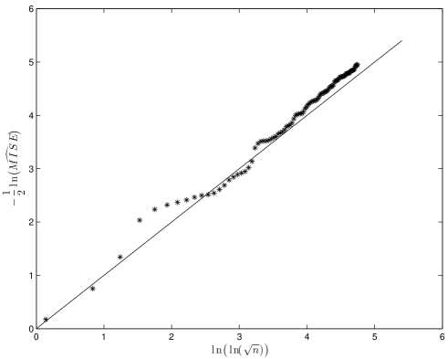
Figure 1: $-\frac{1}{2}\ln\big{(}\widehat{\rm MISE}\big{)}$ plotted against $\ln\big{(}\ln(\sqrt{n})\big{)}$ for $n=10^{k},\;k=1,...,100$ in the case $b=s=1,\alpha=2,\beta=0,\gamma=1$, for fixed $\tau=1$.

In Figure 2 we have $\beta=2$ and all the other parameters the same. The least squares fit gives a slope $0.9723$ with coefficient of determination $0.9916$, confirming that the regularity of the noise as determined by $\beta$ does not affect the rate of convergence.

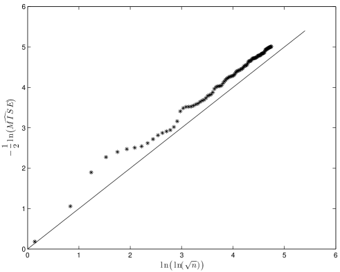
Figure 2: $-\frac{1}{2}\ln\big{(}\widehat{\rm MISE}\big{)}$ plotted against $\ln\big{(}\ln(\sqrt{n})\big{)}$ for $n=10^{k},\;k=1,...,100$ in the case $b=s=1,\alpha=2,\beta=2,\gamma=1$, for fixed $\tau=1$.

Acknowledgmenets. The authors are grateful to Bartek Knapik and Harry Van Zanten for helpful discussions. The authors are also grateful to two referees for several very useful comments.

References

- [1] S. Agapiou, S. Larsson, and A. M. Stuart. Posterior cotraction rates for the Bayesian approach to linear ill-posed inverse problems. Stoch. Proc. Apl., 123(10):3828–3860, 2013.
- [2] L. Cavalier. Nonparametric statistical inverse problems. Inverse Problems, 24(3), 2008.
- [3] Giuseppe Da Prato. An introduction to infinite-dimensional analysis. Universitext. Springer-Verlag, Berlin, 2006. Revised and extended from the 2001 original by Da Prato.
- [4] Giuseppe Da Prato and Jerzy Zabczyk. Stochastic equations in infinite dimensions. Cambridge University Press, Cambridge, 1992.
- [5] P. Diaconis and D. Freedman. On the consistency of Bayes estimates. Ann. Statist., 14(1):1–67, 1986. With a discussion and a rejoinder by the authors.
- [6] Heinz W. Engl, Martin Hanke, and Andreas Neubauer. Regularization of inverse problems. Kluwer Academic Publishers (Dordrecht and Boston), 1996.
- [7] J. N. Franklin. Well-posed stochastic extensions of ill-posed linear problems. J. Math. Anal. Appl., 31:682–716, 1970.
- [8] S. Ghosal, J. K. Ghosh, and A. W. van der Vaart. Convergence rates of posterior distributions. Ann. Statist., 28(2):500–531, 2000.
- [9] T. Hohage. Regularization of exponentially ill-posed problems. Numerical Functional Analysis and Optimization, 21(3-4):439–464, 2000.
- [10] B. T. Knapik, A. W. van der Vaart, and J. H. van Zanten. Bayesian inverse problems with Gaussian priors. Ann. Statist., 39(5):2626–2657, 2011.
- [11] B. T. Knapik, A. W. van der Vaart, and J. H. van Zanten. Bayesian recovery of the initial condition for the heat equation. Comm. Statist. Theory Methods, 42, 2013.
- [12] S. Lasanen. Measurements and infinite-dimensional statistical inverse theory. PAMM, 7:1080101–1080102, 2007.
- [13] S. Lasanen. Non-gaussian statistical inverse problems. Part I: Posterior distributions. Inverse Problems and Imaging, 6(2):215–266, 2012.
- [14] S. Lasanen. Non-gaussian statistical inverse problems. Part II: Posterior distributions. Inverse Problems and Imaging, 6(2):267–287, 2012.
- [15] Peter D. Lax. Linear algebra and its applications. Enlarged second edition. Wiley-Interscience, 2007.
- [16] M. S. Lehtinen, L. Paivarinta, and E. Somersalo. Linear inverse problems for generalised random variables. Inverse Problems, 5(4):599, 1989.
- [17] A. Mandelbaum. Linear estimators and measurable linear transformations on a Hilbert space. Probability Theory and Related Fields, 65:385–397, 1984. 10.1007/BF00533743.
- [18] Y. Pokern, A. M. Stuart, and J. H. van Zanten. Posterior consistency via precision operators for Bayesian nonparametric drift estimation in SDEs. Stoch. Proc. Apl., 123(2):603–628, 2013.
- [19] Franz Schwabl. Quantum mechanics. Springer, Berlin, 2007.
- [20] A. M. Stuart. Inverse problems: A Bayesian perspective. Acta Numerica, 19:451–559, 2010.
- [21] Y.X. Zhang, C.L. Fu, and Z.L. Deng. An a posteriori truncation method for some cauchy problems associated with helmholtz-type equations. Inverse Problems in Science and Engineering, 21(7):1151–1168, 2013.