A Novel Mechanism to Generate FFLO States in Holographic Superconductors

Abstract

We discuss a novel mechanism to set up a gravity dual of FFLO states in strongly coupled superconductors. The gravitational theory utilizes two $U(1)$ gauge fields and a scalar field coupled to a charged AdS black hole. The first gauge field couples with the scalar sourcing a charge condensate below a critical temperature, and the second gauge field provides a coupling to spin in the boundary theory. The scalar is neutral under the second gauge field. By turning on an interaction between the Einstein tensor and the scalar, it is shown that, in the low temperature limit, an inhomogeneous solution possesses a higher critical temperature than the homogeneous case, giving rise to FFLO states.

The AdS/CFT correspondence, which was discovered in string theory, has opened up a broad avenue for the exploration of condensed matter systems at strong coupling. By using a holographic principle, these systems (described by gauge field theories) are mapped onto weakly coupled gravitational systems of one additional dimension, in which physical quantities can be computed. This holographic principle (gauge theory / gravity duality) has been applied to the study of conventional and unconventional superfluids and superconductors HartnollPRL101 , Fermi liquids Bhattacharyya:2008jc , and quantum phase transitions Cubrovic:2009ye .

The high-Tc superconductors, such as cuprates and iron pnictides, are examples of unconventional superconductors which exhibit competing orders that are related to the breaking of the lattice symmetries. This breaking introduces inhomogeneities and a study of the effect of inhomogeneity of the pairing interaction in a weakly coupled BCS system Martin:2005fk suggests that inhomogeneity might play a role in high-Tc superconductivity. In an effort to explain this behavior a “striped” superconductor was proposed Berg:2009fk . Holographic striped superconductors were discussed in Flauger:2010tv where a modulated chemical potential was introduced and it was shown that below a critical temperature superconducting stripes develop. Properties of the striped superconductors and backreaction effects were studied in Hutasoit:2011rd ; Ganguli:2012up . Striped phases were also found in electrically charged RN-AdS black branes that involve neutral pseudo-scalars Donos:2011bh .

Inhomogeneous phases also appear when a strong external magnetic field coupled to the spins of the conduction electrons is applied to a high-field superconductor. This results in a separation of the Fermi surfaces corresponding to electrons with opposite spins (for a review see Casalbuoni:2003wh ). If the separation is too high, the pairing is destroyed and there is a transition from the superconducting state to the normal one (paramagnetic effect). An intriguing new state of matter at the transition point was proposed by Fulde and Ferrell Fulde and Larkin and Ovchinnikov Larkin (the FFLO state) but it has not been found experimentally so far. This state is characterized by a space modulated order parameter, corresponding to an electron pair having nonzero total momentum.

A way to understand the formation of the FFLO phase in a superconductor-ferromagnetic system (S/F) is to use the generalized Ginzburg-Landau expansion. In order to describe the paramagnetic effect in the presence of a strong external magnetic field, the usual $|\psi|^{4}$-Ginzburg-Landau functional has to be modified with coefficients in the functional which depend also on the magnetic field. In this case, the $(B,T)$ phase diagram exhibits a different behavior indicating that the minimum of the functional does not correspond to a uniform state, and a spatial variation of the order parameter decreases the energy of the system. To describe such a situation, it is necessary to add a higher-order derivative term in the expansion of the Ginzburg-Landau functional (for a detailed account see Buzdin:2005zz ).

There are several studies of the behavior of holographic superconductors in the presence of an external magnetic field. Non-trivial spatially dependent solutions have been found, like the droplet Albash:2008eh and vortex solutions with integer winding number Albash:2009iq ; Montull:2009fe ; Maeda:2009vf . An analytic study on holographic superconductors in an external magnetic field was carried out in Ge:2010aa . In a model resulting from a consistent truncation of type IIB string theory, anisotropic solutions at low temperature were found ABKProchazka , showing similarity between the phase diagrams of holographic superfluid flows and those of ordinary superconductors with an imbalanced chemical potential. A holographic superconducting model with unbalanced fermi mixtures at strong coupling was discussed in Bigazzi:2011ak . The charge and spin transport properties of the model were studied, but the phase diagram did not reveal the occurrence of FFLO-like inhomogeneous superconducting phases.

In our recent work Alsup:2012ap , we proposed a gravity dual of FFLO states in strongly coupled superconductors. The gravity sector consisted of two $U(1)$ gauge fields and a scalar field. The first gauge field had a non-zero scalar potential term which was the source of the charge condensate in the boundary theory through its coupling to the scalar field. The second $U(1)$ gauge field corresponded to an effective magnetic field acting on the spins in the boundary theory. The scalar field was neutral under the second $U(1)$ gauge field. We looked first at the behavior of the system at or above the critical temperature. The Eintein-Maxwell system was solved by a dyonic black hole with electric and magnetic charges, as in Bigazzi:2011ak . At the critical temperature, the system underwent a second-order phase transition and the black hole acquired hair. To find the critical temperature, we worked in the grand canonical ensemble and solved the scalar equation in the background of the dyonic black hole. It was found that the system possessed inhomogeneous solutions for the scalar field, which however always gave a transition temperature lower than the maximum transition temperature (i.e. critical temperature) of the homogeneous solution. Therefore the homogeneous solution was always dominant.

Next, we turned on an interaction term of the magnetic field to the scalar field of the generalized Ginzburg-Landau gradient type (in a covariant form). The scalar field equation was modified and the resulting inhomogeneous solutions gave a transition temperature which was higher than the one of the homogeneous solutions. We attributed this behavior of the system to the appearance of FFLO states. We noted that the appearance of the FFLO states was more pronounced as $T_{c}/\mu\rightarrow 0$, and the magnetic field of the second $U(1)$ gauge group was large.

In this letter, we propose a novel mechanism for the generation of the gravity dual of FFLO states in the low temperature limit. In our previous work we showed that, in order to generate the FFLO phase, we needed a direct coupling of the magnetic field to the scalar field. We will show that this interaction term can be effectively generated through the coupling of the Einstein tensor to the scalar field. The reason is that since the electromagnetic fields backreact on the metric, the Einstein tensor has encoded the information of these fields.

As before, the bulk theory consists of two $U(1)$ gauge fields and a scalar field. The first gauge field has a non-zero scalar potential term and the second $U(1)$ gauge field corresponds to a chemical potential (imbalance) for spin. The scalar field is neutral under the second $U(1)$ gauge field. Note, too, the second $U(1)$ is self-dual under $\vec{E}\leftrightarrow\vec{B}$ and alternatively the boundary theory can be understood in terms of a magnetic field instead of the chosen spin chemical potential.

The interaction between the Einstein tensor and the scalar field is most often seen in scalar-tensor theories. The interest stems from the galilean symmetry of the system where the action is invariant under shifts of field derivatives by a constant vector. Thereby the higher-derivative theory has only second order equations of motion galilean . It was shown that this term acts as an effective cosmological constant and produces an early entrance into a quasi-de Sitter stage as well as a smooth exit Sushkov . Cosmic evolution for vanishing cosmological constant has also been investigated in STcosmo . The coupling has been realized in string cosmology from an effective heterotic action, up to $\alpha^{\prime}$ corrections MaedaOhtaWakebe and also in N = 1 four-dimensional new-minimal supergravity theories Farakos:2012je .

Moreover, interest away from cosmology has developed as the interaction has been used to study phase transitions for vanishing cosmological constant Kolyvaris and effects on conventional holographic superconductors employing anti-de Sitter space Chen:2010hi . The presence of this term modifies the scalar field equation and the resulting inhomogeneous solutions give a transition temperature which is higher than the homogeneous solutions. We attribute this behavior to FFLO states. Note that as before, the appearance of the FFLO states is more pronounced as $T_{c}/\mu\rightarrow 0$ and the gauge field of the second $U(1)$ gauge group is near its maximum value.

Consider the action

$$S =$$

$$\int d^{4}x\sqrt{-g}\left[\frac{R+6/L^{2}}{16\pi G}-\frac{1}{4}F_{AB}F^{AB}-\frac{1}{4}\mathcal{F}_{AB}\mathcal{F}^{AB}\right],$$

where $F_{AB}=\partial_{A}A_{B}-\partial_{B}A_{A}$, $\mathcal{F}_{AB}=\partial_{A}\mathcal{A}_{B}-\partial_{B}\mathcal{A}_{A}$ are the field strengths of the $U(1)$ potentials $A_{A}$ and $\mathcal{A}_{A}$, respectively. We set $L=8\pi G=1$.

The Einstein-Maxwell equations,

$$R_{\mu\nu} - \frac{1}{2}g_{\mu\nu}R-\frac{3}{L^{2}}g_{\mu\nu}=$$

$$\frac{1}{2}\big{[}F_{\mu\sigma}F^{\sigma}_{\nu}-\frac{1}{4}g_{\mu\nu}F^{2}+\mathcal{F}_{\mu\sigma}\mathcal{F}^{\sigma}_{\nu}-\frac{1}{4}g_{\mu\nu}\mathcal{F}^{2}\big{]},$$

$$\nabla_{\mu} F {}^{\mu\nu}=0,$$

$$\nabla_{\mu} \mathcal{F} {}^{\mu\nu}=0,$$ (2)

admit a solution which is a four-dimensional AdS black hole of two $U(1)$ charges,

$$ds^{2}=\frac{1}{z^{2}}\left[-h(z)dt^{2}+\frac{dz^{2}}{h(z)}+dx^{2}+dy^{2}\right],$$ (3)

with the horizon radius set at $z=1$.

The two sets of Maxwell equations admit solutions of the form, respectively,

$$A_{t}=\mu\left(1-z\right)\ ,\ \ A_{z}=A_{x}=A_{y}=0,$$ (4)

and

$$\mathcal{A}_{t}=\delta\mu(1-z)\ ,\ \ \mathcal{A}_{z}=\mathcal{A}_{x}=\mathcal{A}_{y}=0,$$ (5)

with corresponding field strengths having non-vanishing components for electric fields in the $z$-direction, respectively,

$$F_{tz}=-F_{zt}=\mu\ \ ,\ \ \ \ \mathcal{F}_{tz}=-\mathcal{F}_{zt}=\delta\mu~{}.$$ (6)

Then from the Einstein equations we obtain

$$h(z)=1-\left(1+\frac{\mu^{2}+\delta\mu^{2}}{4}\right)z^{3}+\frac{\mu^{2}+\delta\mu^{2}}{4}z^{4}~{}.$$ (7)

The Hawking temperature is

$$T=-\frac{h^{\prime}(1)}{4\pi}=\frac{3}{4\pi}\left[1-\frac{\mu^{2}+\delta\mu^{2}}{12}\right].$$ (8)

In the limit $\mu,\delta\mu\to 0$ we recover the Schwarzschild black hole.

Next, we consider a scalar field $\phi$, of mass $m$, and $U(1)^{2}$ charge $(q,0)$, coupled to the Einstein tensor. The action is

$$S= - \int d^{4}x\sqrt{-g}\Big{[}g^{AB}(D_{A}\phi)^{\ast}D_{B}\phi+m^{2}(1-3\xi)|\phi|^{2}$$ (9)

$$- \xi G^{AB}(D_{A}\phi)^{\ast}D_{B}\phi\Big{]},$$

where $D_{A}=\partial_{A}+iqA_{A}$ and $G_{AB}$ is the Einstein tensor. $\xi$ is the new coupling constant determining the strength of the interaction between the scalar field and the Einstein tensor. We also included a convenient $\xi$-dependent factor in the mass term. We shall consider the range of $\xi$ for which the factor is positive,

$$\xi<\frac{1}{3}~{}.$$ (10)

Firstly, we consider the conventional case setting $\xi=0$. The asymptotic behavior (as $z\to 0$) of the scalar field is

$$\phi\sim z^{\Delta}\ \ ,\ \ \ \ \Delta(\Delta-3)=m^{2}~{}.$$ (11)

For $m^{2}\geq-5/4$, there is only one normalizable mode. However, for the range, $-9/4\leq m^{2}<-5/4$, there are two allowable choices of $\Delta$,

$$\Delta=\Delta_{\pm}=\frac{3}{2}\pm\sqrt{\frac{9}{4}+m^{2}}~{},$$ (12)

leading to two distinct physical systems.

As we lower the temperature, an instability arises and the system undergoes a second-order phase transition with the black hole developing hair. This occurs at a critical temparture $T_{c}$ which is found by solving the scalar wave equation in the above background,

$$\partial_{z}^{2}\phi+\left[\frac{h^{\prime}}{h}-\frac{2}{z}\right]\partial_{z}\phi+\frac{1}{h}\nabla_{2}^{2}\phi-\frac{1}{h}\left[\frac{m^{2}}{z^{2}}-q^{2}\frac{A_{t}^{2}}{h}\right]\phi=0,$$ (13)

with the metric function $h$ given in (7) and the electrostatic potential $A_{t}$ in (4).

Although the wave equation (13) possesses $(x,y)$-dependent solutions, the symmetric solution dominates and the hair that forms has no $(x,y)$ dependence. To see this, let us introduce $(x,y)$-dependence and consider a static scalar field which is an eigenstate of the two-dimensional Laplacian,

$$\nabla_{2}^{2}\phi=-\tau\phi\ \ ,\ \ \ \ \tau>0~{}.$$ (14)

For example, if $\phi$ varies sinusoidally in the $x$-direction, $\phi\sim e^{iQx}$, then $\tau=Q^{2}$ and the modulation is realized in the boundary CFT through the order parameter $\langle\mathcal{O}\rangle\sim e^{iQx}$. It is also possible for $\phi$ to be rotationally symmetric in the $(x,y)$ plane, $\phi\sim J_{0}(\sqrt{\tau(x^{2}+y^{2})})$. For $\tau=0$, we recover the homogeneous solution.

Upon factoring out the $(x,y)$ dependence,

$$\phi=Y(x,y)\psi(z)~{},$$ (15)

where $Y(x,y)$ is an eigenfunction of the two-dimensional Laplacian with eigenvalue $-\tau$ (eq. (14)), the scalar field is represented by $\psi(z)$ and the wave equation becomes

$$\psi^{\prime\prime}+\left[\frac{h^{\prime}}{h}-\frac{2}{z}\right]\psi^{\prime}-\frac{\tau}{h}\psi-\frac{1}{h}\left[\frac{m^{2}}{z^{2}}-q^{2}\frac{A_{t}^{2}}{h}\right]\psi=0.$$ (16)

Before we proceed with a discussion of solutions, notice that there is a scaling symmetry

$$z \ \to\lambda z\ ,\ \ x\to\lambda x\ ,\ \ \tau\to\tau/\lambda^{2}\ ,$$

$$\mu \ \to\mu/\lambda\ ,\ \ \delta\mu\to\delta\mu/\lambda\ ,\ \ T\to T/\lambda~{}.$$ (17)

This means that the system possesses a scale which we have fixed for simplicity of notation. This arbitrary scale is often taken to be the radius of the horizon $r_{+}$, after changing coordinates to

$$z=\frac{r_{+}}{r}~{}.$$ (18)

Since we fixed the scale, we should only be reporting on scale-invariant quantities, such as $T/\mu$, $\delta\mu/\mu$, $\tau/\mu^{2}$, etc. It is also convenient to introduce the scale-invariant parameter

$$\beta=\frac{\delta\mu}{\mu}$$ (19)

to describe the effect of the chemical potential imbalance.

We shall be working in the grand canonical ensemble at fixed chemical potentials $\mu$ and $\delta\mu$ (or $\beta$). The ensemble is defined uniquely by specifying the parameters $q$ and $\Delta$. One can then vary $\tau$, which parametrizes the solutions, to study the behavior of the system.

Since we fixed the scale, we shall solve the wave equation (16) for fixed values of the scale-invariant parameters $\tau/\mu^{2}$ and $\beta$, while demanding regularity at the horizon and $\psi\sim z^{\Delta_{+}}$ at the boundary. Thus, we obtain $\mu=\mu_{0}$ as an eigenvalue. More precisely, we obtain $\mu/r_{+}$ as an eigenvalue, where $r_{+}$ is the scale in the system. Since the chemical potential $\mu$ is fixed (grand canonical ensemble), the solution of the wave equation (16) fixes the scale ($r_{+}=r_{+0}$, so that $\mu_{0}\to\mu/r_{+0}$) , and therefore the transition temperature $T_{0}$ below which a mode with the given $\tau$ may develop. We obtain

$$\frac{T_{0}}{\mu_{\mathrm{eff}}}=\frac{3}{4\pi\mu_{\mathrm{eff,0}}}\left[1-\frac{\mu_{\mathrm{eff,0}}^{2}}{12}\right]~{},$$ (20)

which is of the same form as a Reissner-Nordström black hole with effective chemical potential

$$\mu_{\mathrm{eff}}^{2}=\mu^{2}(1+\beta^{2})~{}.$$ (21)

The maximum transition temperature is the critical temperature $T_{c}$ of the system. As we cool down the system in its normal state, the transition temperature $T_{0}=T_{c}$ is reached first and the mode with the corresponding $\tau$ is the first to develop.

In the homogeneous case, $\tau=0$, the maximum transition temperature is obtained for $\beta=0$. In this case, we recover the Reissner-Nordström black hole. As we increase $\beta$, the temperature (20) decreases. The scalar wave equation is the same as its counterpart in a Reissner-Nordström background, but with effective charge

$$q_{\mathrm{eff}}^{2}=\frac{q^{2}}{1+\beta^{2}}~{},$$ (22)

so that $q_{\mathrm{eff}}\mu_{\mathrm{eff}}=q\mu$.

It is known HartnollPRL101 that the instability Breitenlohner:1982jf occurs for all values of $q_{\mathrm{eff}}$, including $q_{\mathrm{eff}}=0$, if $\Delta\leq\Delta_{\ast}$, where $\Delta_{\ast}=\Delta_{+}$ for $m^{2}=-\frac{3}{2}$, or explicitly,

$$\Delta_{\ast}=\frac{3+\sqrt{3}}{2}\approx 2.366~{}.$$ (23)

For $\Delta\leq\Delta_{\ast}$, $\beta$ can increase indefinitely. The transition temperature $T_{0}$ for $\tau=0$ has a minimum value as a function of $\beta$, and as $\beta\to\infty$, $T_{0}$ diverges.

For $\Delta>\Delta_{\ast}$, $q_{\mathrm{eff}}$ has a minimum value at which the transition temperature vanishes and the black hole attains extremality. This is found by considering the limit of the near horizon region Horowitz:2009ij ; AST . One obtains

$$q_{\mathrm{eff}}\geq q_{\mathrm{min}}\ \ ,\ \ \ \ q_{\mathrm{min}}^{2}=\frac{3+2\Delta(\Delta-3)}{4}.$$ (24)

At the minimum ($T_{0}=0$), $\mu_{\mathrm{eff}}^{2}=12$, and $\beta$ attains its maximum value,

$$\beta\leq\beta_{\mathrm{max}}\ \ ,\ \ \ \ \beta_{\mathrm{max}}^{2}=\frac{q^{2}}{q_{\mathrm{min}}^{2}}-1~{}.$$ (25)

This limit is reminiscent of the Chandrasekhar and Clogston limit instability in a S/F system, in which a ferromagnet at $T=0$ cannot remain a superconductor with a uniform condensate.

In the inhomogeneous case ($\tau\neq 0$), the above argument still holds with the replacement $m^{2}\to m^{2}+\tau$. The effect of this modification is to increase the minimum effective charge to

$$q_{\mathrm{min}}^{2}=\frac{3+2\Delta(\Delta-3)+2\tau}{4},$$ (26)

and thus decrease the maximum value of $\beta$ (25). We always obtain a transition temperature which is lower than the corresponding transition temperature (for same $\beta$) in the homogeneous case ($\tau=0$). It follows that the critical temperature is the transition temperature of the homogeneous mode, and the latter dominates the condensate.

Notice also that $\tau\leq\tau_{\mathrm{max}}$, where the maximum value is attained when $q_{\mathrm{min}}=q$ (so that $\beta_{\mathrm{max}}=0$). We deduce from (26),

$$\tau_{\mathrm{max}}=2q^{2}-\frac{3}{2}-\Delta(\Delta-3)~{}.$$ (27)

The supporting numerical results are shown in figure 1.

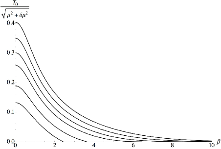
Figure 1: The transition temperature for various modes $vs.$ $\beta$ numerically calculated with $q=10$, $\Delta=5/2$, and $\xi=0$. Starting from the top, on the vertical axis, the lines are $\frac{\tau}{(q\mu)^{2}}=0$ (the critical temperature of the system), $.05,~{}.10,~{}.15,~{}.25,$ and $.35$.

Now let us consider the effect of coupling to the Einstein tensor by setting $\xi\neq 0$. The wave equation is modified to

$$\psi^{\prime\prime}+\left[\frac{h^{\prime}}{h}+\frac{f_{+}^{\prime}}{f_{+}}-\frac{2}{z}\right]\psi^{\prime}-\frac{\tau}{h}\,\frac{f_{-}}{f_{+}}\psi$$

$$-\frac{1}{h}\left[\frac{m^{2}(1-3\xi)}{z^{2}f_{+}}-q^{2}\frac{A_{t}^{2}}{h}\right]\psi = 0~{},$$ (28)

where

$$f_{\pm}=1-3\xi\pm\xi\frac{\mu_{\mathrm{eff}}^{2}}{4}z^{4}~{}.$$ (29)

Note that the boundary behavior is unaltered from (12).

The coupling to the Einstein tensor alters the near horizon limit of the theory so that

$$m^{2}\to\frac{m^{2}(1-3\xi)+\tau f_{-}(1)}{f_{+}(1)}~{},$$ (30)

For $\xi<1/6$, it is easily seen from (29) that $f_{\pm}(1)>0$, so that the effective mass increases with $\tau$, as in the conventional $\xi=0$ case.

The minimum effective charge is found from the near-horizon geometry in the zero temperature (extremal) limit. Using $\mu_{\mathrm{eff}}^{2}=12$ and $f_{\pm}(1)=1-3\xi\pm 3\xi$, we obtain

$$q_{\mathrm{min}}^{2}=\frac{3+2(1-3\xi)\Delta(\Delta-3)+2(1-6\xi)\tau}{4}~{},$$ (31)

to be compared with (26).

Finally, $\tau$ has a maximum value found by setting $q_{\mathrm{min}}=q$ in (31),

$$\tau_{\mathrm{max}}=\frac{2q^{2}-\frac{3}{2}-(1-3\xi)\Delta(\Delta-3)}{1-6\xi}~{}.$$ (32)

Thus, for $\xi<1/6$, even though the results differ numerically from the case $\xi=0$, they are not qualitatively different. The maximum transition temperature (i.e., the critical temperature of the system) is always attained for $\tau=0$ (homogeneous case). As $\xi$ approaches the critical value $\frac{1}{6}$, the maximum value of $\tau$ diverges.

As we increase $\xi$ past the critical value, i.e., for

$$\xi>1/6~{},$$ (33)

(with $\xi$ still satisfying (10)), the range of $\tau$ extends to infinity ($\tau_{\mathrm{max}}$ is infinite), and the behavior of the system changes qualitatively. For $\xi$ above the bound (33), the minimum charge decreases for $\tau>0$, and therefore the maximum value of $\beta$ (25) increases compared to the value in the homogeneous case ($\tau=0$). Thus, there is a neighborhood near zero temperature in which the inhomogeneous solution has higher transition temperature than the homogeneous one. As we increase $\tau$, the corresponding transition temperature increases. This expected behavior is also seen numerically.

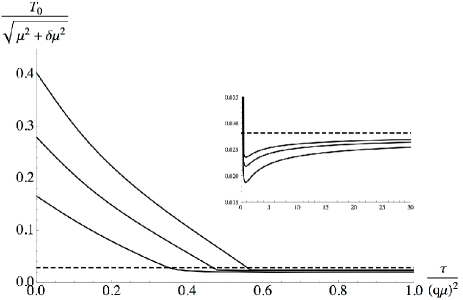
Figure 2: The top of the graph corresponds to $\beta=0$, with lines $\beta=1,2$ below for all values of $\tau$. The transition temperature of the homogeneous solution ($\tau=0$) is found to be the largest for this range of $\beta$. We used $q=10$, $\Delta=5/2$, and $\xi=.20$. The dotted line represents the asymptotic value for the transition temperature (35). The inset is an enlarged view of the lines as they approach the asymptotic (critical) temperature.

As we keep increasing $\tau$, we are no longer in the zero temperature limit and geometrical considerations near the horizon are no longer applicable. Thus, although the effective mass (30) keeps decreasing below the AdS₂ BF bound, the latter is no longer relevant, and the wave equation possesses acceptable solutions for all $\tau$. Although we can no longer argue analytically, we analyzed the behavior of the system numerically. As $\tau$ increases, the corresponding transition temperature keeps increasing. The maximum transition temperature, which would be identified with the critical temperature of the system, is attained asymptotically as $\tau\to\infty$ (recall that there is no maximum value of $\tau$ for $\xi>1/6$).

The value of the critical temperature is found by analytically solving the wave equation in the limit $\tau\to\infty$. It is easy to see by considering an expansion around the horizon that we ought to have $f_{-}=0$. We deduce

$$\mu_{\mathrm{eff,c}}^{2}=\frac{4(1-3\xi)}{\xi}~{},$$ (34)

thus determining the asymptotic transition (critical) temperature to be

$$\lim_{\tau/\mu^{2}\to\infty}\frac{T_{c}}{\mu_{\mathrm{eff}}}\to\frac{3}{4\pi}\sqrt{\frac{\xi}{1-3\xi}}\left(1-\frac{1}{6\xi}\right),$$ (35)

which is dependent solely upon our coupling constant $\xi$.

To find the critical temperature numerically (and confirm the analytic prediction (35)), we fix the chemical potentials $\mu$ and $\delta\mu$ (or $\beta$) and numerically solve the wave equation (A Novel Mechanism to Generate FFLO States in Holographic Superconductors) for all allowed values of $\tau$. Figure 2 displays the transition temperatures of various modes for small values $\beta$. The plots attain their maximum at the homogeneous mode, $\tau=0$, and therefore the homogeneous solution is dominant. The low temperature region is probed with larger values of $\beta$. Our results are plotted in figure 3. The homogeneous solution possesses a transition temperature that is below the majority of non-zero $\tau$ and hence the inhomogeneous solutions dominate.

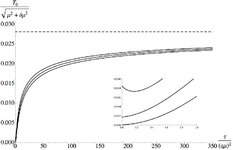
Figure 3: The lines, from top to bottom represent $\beta=11.5,12.5,13.5$ with $q=10$, $\Delta=5/2$, and $\xi=.20$. The transition temperature of the homogeneous solution ($\tau=0$) is less than that of $\tau/\mu^{2}\to\infty$. The dotted line represents the asymptotic value for the temperature (35) (critical temperature). The inset shows the curves for small $\tau$.

As we increase $\tau$, the corresponding transition temperature increases and approaches the asymptotic value (35), as expected. The asymptotic value (critical temperature) is an upper bound for the transition temperatures of the various modes.

Figure 4 displays the transition temperature numerically calculated for $\xi=.2$ for select values of $\tau$. The point where the inhomogeneous solution becomes dominant is found at the crossing between $\tau=0$ and the large $\tau$ asymptotic (critical) temperature seen in the body of the figure.

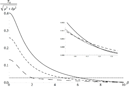
Figure 4: The transition temperature of various modes $vs.$ $\beta$ numerically calculated with $q=10$ and $\Delta=5/2$, and $\xi=.20$. Starting from the top, on the vertical axis, the lines are $\frac{\tau}{(q\mu)^{2}}=0,~{}.15,$ and $.35$, followed by the dash-dotted line representing the asymptotic value for the transition temperature. The crossing between the finite values $\tau$ is shown in the inset.

In a condensed matter system with an order parameter possessing wavenumber $Q$, the lattice spacing $a$ is related by $Q\sim 1/a$ Casalbuoni:2003wh . In our system, effectively $a\to 0$, which corresponds to $\tau=Q^{2}\to\infty$. Therefore, we expect the critical temperature to correspond to $\tau\to\infty$. It would be desirable to include lattice effects so that the critical temperature corresponds to a large but finite value of $\tau$ latticeDrude ; latticeFermion . An effective way of accomplishing this is by including higher order terms in the Lagrangian. Let us introduce a cutoff that suppresses large momentum ($\tau$) modes in the Einstein coupling term. To do this covariantly, introduce the derivative operator

$$\mathcal{D}^{A}=\frac{1}{2}\epsilon^{ABCD}\mathcal{F}_{BC}D_{D}~{},$$ (36)

where $\mathcal{F}$ is the field strength of the second $U(1)$ potential, and $D_{A}$ is the gauge derivative (see eq. (9)). Then modify the action for the scalar field (9) to

$$S= - \int d^{4}x\sqrt{-g}\Big{[}g^{AB}(D_{A}\phi)^{\ast}D_{B}\phi+m^{2}(1-3\xi)|\phi|^{2}$$ (37)

$$- \frac{\xi}{2}G^{AB}(D_{A}\phi)^{\ast}D_{B}\mathcal{S}\left(-\alpha\mathcal{D}_{A}\mathcal{D}^{A}\right)\phi+\mathrm{c.c.}\Big{]}.$$

The function $\mathcal{S}(x)$ is chosen so that $\mathcal{S}(0)=1$ and $\mathcal{S}(x)\to 0$, as $x\to\infty$. We also introduced a new (small) parameter $\alpha$. It is convenient to choose

$$\mathcal{S}(x)=e^{-x}~{}.$$ (38)

The wave equation (A Novel Mechanism to Generate FFLO States in Holographic Superconductors) is modified to

$$\psi^{\prime\prime}+\left[\frac{h^{\prime}}{h}+\frac{f_{+}^{\prime}}{f_{+}}-\frac{2}{z}\right]\psi^{\prime}-\frac{\tau}{h}\,\frac{f_{-}}{f_{+}}\psi$$

$$-\frac{1}{h}\left[\frac{m^{2}(1-3\xi)}{z^{2}f_{+}}-q^{2}\frac{A_{t}^{2}}{h}\right]\psi$$

$$-3\alpha\beta^{2}\mu^{2}\tau z^{5}\left[\left(\frac{h^{\prime}}{h}+\frac{3}{z}\right)\left(1-\frac{1}{f_{+}}\right)+\frac{f_{+}^{\prime}}{f_{+}}\right]\psi = 0~{},\ \ \ \$$ (39)

and the functions $f_{\pm}$ (eq. (29)) are modified to

$$f_{\pm}=1+\xi\left[-3\pm\frac{\mu_{\mathrm{eff}}^{2}}{4}z^{4}\right]e^{-\alpha\beta^{2}\mu^{2}\tau z^{6}}~{}.$$ (40)

Notice that in the limit $\tau\to\infty$, we have $f_{\pm}\to 1$, so for large $\tau$, the solutions approach those in the standard case $\xi=0$, in which there is a maximum allowed value of $\tau$ (eq. (27)). The supporting numerics are shown in figure 5, where a maximum transition temperature (critical temperature) at finite $\tau$ may be clearly seen.

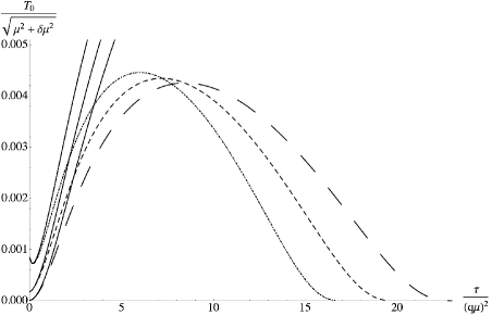
Figure 5: The lines, from top to bottom on the left side represent transition temperature for various modes with $\beta=11.5,12.5,13.5$ with $q=10$, $\Delta=5/2$, $\xi=.20$. The solid lines correspond to the $\alpha=0$ solutions while the dashed lines correspond to the cutoff solution with $\alpha=.0001$. The dot-dashed line is for $\beta=11.5$, the short dashes are used for $\beta=12.5$, and long dashes for $\beta=13.5$.

In conclusion, we have developed a gravitational dual theory for the FFLO state of condensed matter. The gravitational theory consists of two $U(1)$ gauge fields and a scalar coupled to a charged AdS black hole. The first gauge field produces the instability for a condensate to form, while the second controls chemical potential associated with spin. In the absence of an interaction of the Einstein tensor with the scalar field, the system possesses dominant homogeneous solutions for all allowed values of the spin chemical potential. In the presence of the interaction term, at low temperatures, the system is shown to possess a critical temperature for a transition to a scalar field with spatial modulation as opposed to the homogeneous solution.

It is desirable to fully understand the interplay between the different modes once below the critical temperature. This will require a non-linear analysis of the Einstein-Maxwell-scalar equations. Additionally, the dependence of the critical temperature on the modulation wavenumber, which is intertwined with the presence of a lattice is an intriguing aspect. Work in these directions is in progress.

- (1) S. A. Hartnoll, C. P. Herzog, and G. T. Horowitz, Phys. Rev. Lett. 101, 031601 (2008); S. A. Hartnoll, C. P. Herzog, and G. T. Horowitz, JHEP 0812, 015 (2008).
- (2) S. Bhattacharyya, V. E. Hubeny, S. Minwalla and M. Rangamani, JHEP 0802, 045 (2008).
- (3) M. Cubrovic, J. Zaanen and K. Schalm, Science 325, 439 (2009).
- (4) I. Martin, D. Podolsky, and S. A. Kivelson, Phys. Rev. B 72 (2005) 060502.
- (5) E. Berg, E. Fradkin, S. A. Kivelson, and J. Tranquada, New J. Phys. 11 (2009) 115004.
- (6) R. Flauger, E. Pajer and S. Papanikolaou, Phys. Rev. D 83, 064009 (2011).
- (7) J. A. Hutasoit, S. Ganguli, G. Siopsis and J. Therrien, JHEP 1202, 086 (2012).
- (8) S. Ganguli, J. A. Hutasoit and G. Siopsis, arXiv:1205.3107 [hep-th].
- (9) A. Donos and J. P. Gauntlett, JHEP 1108, 140 (2011).
- (10) R. Casalbuoni and G. Nardulli, Rev. Mod. Phys. 76, 263 (2004).
- (11) P. Fulde and R. A. Ferrell, Phys. Rev. 135, A550 (1964).
- (12) A. I. Larkin and Y. N. Ovchinnikov, Zh. Eksp. Teor. Fiz. 47, 1136 (1964) [Sov. Phys. JETP 20, 762 (1965)].
- (13) A. I. Buzdin, Rev. Mod. Phys. 77, 935 (2005).
- (14) T. Albash and C. V. Johnson, JHEP 0809, 121 (2008).
- (15) T. Albash and C. V. Johnson, Phys. Rev. D 80, 126009 (2009); T. Albash and C. V. Johnson, arXiv:0906.0519 [hep-th].
- (16) M. Montull, A. Pomarol and P. J. Silva, Phys. Rev. Lett. 103, 091601 (2009).
- (17) K. Maeda, M. Natsuume and T. Okamura, Phys. Rev. D 81, 026002 (2010).
- (18) X. -H. Ge, B. Wang, S. -F. Wu and G. -H. Yang, JHEP 1008, 108 (2010).
- (19) D. Arean, M. Bertolini, C. Krishnan, and T. Prochazka, JHEP 1109, 131 (2011).
- (20) F. Bigazzi, A. L. Cotrone, D. Musso, N. P. Fokeeva and D. Seminara, JHEP 1202, 078 (2012).
- (21) J. Alsup, E. Papantonopoulos and G. Siopsis, arXiv:1208.4582 [hep-th].
- (22) A. Nicolis, R. Rattazzi, and E. Trincherini, Phys. Rev. D 79, 064036 (2009);
- (23) S. V. Sushkov, Phys. Rev. D 80, 103505 (2009).
- (24) E. N. Saridakis, S. V. Sushkov Phys. Rev. D 81, 083510 (2010); C. Germani, A. Kehagias, Phys. Rev. Lett. 105, 011302 (2010).
- (25) K. Maeda, N. Ohta, and R. Wakebe, Eur. Phys. J. C 72 1949 (2012).
- (26) F. Farakos, C. Germani, A. Kehagias and E. N. Saridakis, JHEP 1205, 050 (2012).
- (27) T. Kolyvaris, G. Koutsoumbas, E. Papantonopoulos, and G. Siopsis, Class. Quant. Grav. 29, 205011 (2012).
- (28) S. Chen, Q. Pan and J. Jing, Chin. Phys. B 21, 040403 (2012) [arXiv:1012.3820 [gr-qc]].
- (29) P. Breitenlohner and D. Z. Freedman, Annals Phys. 144, 249 (1982).
- (30) G. T. Horowitz and M. M. Roberts, JHEP 0911, 015 (2009).
- (31) J. Alsup, G. Siopsis, and J. Therrien, Phys. Rev. D 86, 025002 (2012).
- (32) B. S. Chandrasekhar, Appl. Phys. Lett. 1, 7 (1962). A. M. Clogston, Phys. Rev. Lett. 9, 266 (1962).
- (33) G. Horowitz, J. Santos, and D. Tong, JHEP 1207, 168 (2012); G. Horowitz, J. Santos, and D. Tong, JHEP 1211, 102 (2012).
- (34) Y. Liu, K. Schalm, Y. Sun, J. Zaanen, JHEP 1210, 036 (2012).