The Hofer question on intermediate symplectic capacities

Abstract.

Roughly twenty five years ago Hofer asked: can the cylinder ${\rm B}^{2}(1)\times\mathbb{R}^{2(n-1)}$ be symplectically embedded into ${\rm B}^{2(n-1)}(R)\times\mathbb{R}^{2}$ for some $R>0$? We show that this is the case if $R\geqslant\sqrt{2^{n-1}+2^{n-2}-2}$. We deduce that there are no intermediate capacities, between $1$-capacities, first constructed by Gromov in 1985, and $n$-capacities, answering another question of Hofer. In 2008, Guth reached the same conclusion under the additional hypothesis that the intermediate capacities should satisfy the exhaustion property.

1. Introduction

A symplectic manifold is a pair $(M,\omega)$ consisting of a $2n$-dimensional ${\rm C}^{\infty}$-smooth manifold $M$ and a symplectic form $\omega$, that is, a non-degenerate closed differential $2$-form on $M$. For instance, any open subset of $\mathbb{R}^{2n}$ equipped with the $2$-form $\omega_{0}=\sum_{i=1}^{n}{\rm d}x_{i}\wedge{\rm d}y_{i},$ where $(x_{1},y_{1},\ldots,x_{n},y_{n})$ denote the coordinates in $\mathbb{R}^{2n}$, is a symplectic manifold. If $U$ and $V$ are open subsets of $\mathbb{R}^{2n}$, a symplectic embedding $f\colon U\to V$ is a smooth embedding such that $f^{*}\omega_{0}=\omega_{0}.$ In particular, ${\rm volume}(U)\leqslant{\rm volume}(V)$.

Let ${\rm B}^{2n}(R)$ denote the open ball of radius $R$ in $\mathbb{R}^{2n}$, where $R>0$, that is, the set of points $(x_{1},y_{1}\ldots,x_{n},y_{n})\in\mathbb{R}^{2n}$ such that $\sum_{i=1}^{n}(x_{i})^{2}+(y_{i})^{2}<R^{2}$. Gromov’s Nonsqueezing Theorem [9] states that there is no symplectic embedding of ${\rm B}^{2n}(1)$ into the cylinder ${\rm B}^{2}(R)\times\mathbb{R}^{2(n-1)}$ for $R<1$.

Coming from the variational theory of Hamiltonian dynamics, Ekeland and Hofer gave a proof of Gromov’s Nonsqueezing Theorem by studying periodic solutions of Hamiltonian systems.

1.1. Embeddings

Hofer asked [12, page 17]: is there $R>0$, such that the cylinder ${\rm B}^{2}(1)\times\mathbb{R}^{2(n-1)}$ symplectically embeds into ${\rm B}^{2(n-1)}(R)\times\mathbb{R}^{2}$?

Theorem 1.1.

If $n\geqslant 2$, the cylinder ${\rm B}^{2}(1)\times\mathbb{R}^{2(n-1)}$ may be symplectically embedded into the product ${\rm B}^{2(n-1)}(R)\times\mathbb{R}^{2}$ for all $R\geqslant\sqrt{2^{n-1}+2^{n-2}-2}$.

Guth’s work ([10, Section 2], [11, Section 1]) answers the bounded version of the question by producing symplectic embeddings from ${\rm B}^{2}(1)\times{\rm B}^{2(n-1)}(S)$, for any $S>0$, into ${\rm B}^{4}(R)\times{\mathbb{R}}^{2(n-2)}$ for some $R>0$. The proof of Theorem 1.1 builds on works of Guth, Hind, Kerman, and Polterovich.

1.2. Capacities

Ekeland and Hofer’s point of view on Gromov’s Nonsqueezing turned out to be powerful, and allowed them to construct infinitely many new symplectic invariants, called symplectic capacities [5, 12, 13]. For each integer $1\leqslant d\leqslant n$, one can define the notion a symplectic $d$-capacity (see Section 2). Whether given $d$, one can construct a symplectic $d$-capacity is not clear. The first symplectic $1$-capacity was constructed by Gromov himself, it is called the Gromov radius:

$${\rm c}_{{\rm GR}}(M,\omega):=\sup\{r>0\,\,|\,\,{\rm exists\,\,symplectic\,\,embedding}\,\,{\rm B}^{2n}(r)\hookrightarrow M\}.$$

The fact that the Gromov radius is a symplectic $1$-capacity is equivalent to Gromov’s Nonsqueezing theorem. The volume induced by the symplectic form provides an example of symplectic $n$-capacity. Symplectic $d$-capacities are called intermediate capacities when $1<d<n$. In [12, page 17], four years after Gromov’s work, Hofer predicts the nonexistence of intermediate capacities. We’ll prove the prediction of Hofer:

Theorem 1.2.

Let $n\geqslant 3$. If $1<d<n$, symplectic $d$-capacities do not exist on any subcategory of the category of $2n$-dimensional symplectic manifolds.

The so called $d$-nontriviality property of $d$-capacities (see Section 2, item (3)) cannot be satisfied if $1<d<n$ because of Theorem 1.1. Hence Theorem 1.1 implies Theorem 1.2. Guth proved [10] that intermediate capacities which also satisfy the exhaustion property (the value of the capacity on an open set equals the supremum of the values on its compact subsets) do not exist (see Latschev [17] and Remark 2).

Remark 1.3. Theorem 1.2 implies, in view of Gromov’s theorem, that symplectic $d$-capacities exist if and only if $d\in\{1,\,n\}$. Theorem 1.1 is a “squeezing statement”: an arbitrarily large ${\mathbb{R}}^{N}$ may be squeezed into ${\mathbb{R}}^{2}$ provided there is a bounded component whose size can be increased to make room. This is in agreement with the fact that $1$-capacities exist due to non-squeezing, while $d$-capacities ($1<d<n$) do not exist due to squeezing. $\oslash$

The literature on the subject is extensive, and we refer to [4, 8, 14, 15, 27, 28] and the references therein.

2. Symplectic capacities

Symplectic capacities were invented in Ekeland and Hofer’s influential paper [5, 12]. The first capacity, called the Gromov radius, was constructed by Gromov [9] (its existence follows from the Nonsqueezing Theorem). For the basic notions concerning symplectic capacities we refer to [4]. We follow the presentation therein here. Denote by $\mathcal{E}\ell\ell$ the category of ellipsoids in $\mathbb{R}^{2n}$ with symplectic embeddings induced by global symplectomorphisms of $\mathbb{R}^{2n}$ as morphisms, and by ${\rm Symp}^{2n}$ the category of all symplectic manifolds of dimension $2n$, with symplectic embeddings as morphisms. A symplectic category is a subcategory $\mathcal{C}$ of ${\rm Symp}^{2n}$ such that $(M,\omega)\in\mathcal{C}$ implies that $(M,\lambda\omega)\in\mathcal{C}$ for all $\lambda>0$. A generalized symplectic capacity on a symplectic category $\mathcal{C}$ is a functor $c$ from $\mathcal{C}$ to the category $([0,\infty],\leqslant)$ satisfying the following two axioms:

• Monotonicity: $c(M,\omega)\leqslant c(M^{\prime},\omega^{\prime})$ if there exists a morphism from $(M,\omega)$ to $(M,\omega^{\prime})$ (this is a reformulation of “functoriality”);

• Conformality: $c(M,\lambda\omega)=\lambda c(M,\omega)$ for all $\lambda>0$.

A symplectic capacity is a generalized symplectic capacity which, in addition to (1) and (2), is required to satisfy nontriviality:

$$c({\rm B}^{2n}(1))>0\,\,\,\,\,\,\textup{and}\,\,\,\,\,\,\,c({\rm B}^{2}(1)\times\mathbb{R}^{2n-2})<\infty,$$

and the normalization property (that is $c({\rm B}^{2n}(1))=1$). Now let’s consider a symplectic category $\mathcal{C}\subset{\rm Symp}^{2n}$ which contains $\mathcal{E}\ell\ell$ and let $1\leqslant d\leqslant n$. A symplectic $d$-capacity on $\mathcal{C}$ is a generalized capacity satisfying:

• $d$-nontriviality: $c(B^{2n}(1))>0$ and

  $$\begin{cases}c({\rm B}^{2d}(1)\times\mathbb{R}^{2(n-d)})<\infty\\ c({\rm B}^{2(d-1)}(1)\times\mathbb{R}^{2(n-d+1)})=\infty\\ \end{cases}$$

Symplectic $d$-capacities are often called intermediate capacities if $2\leqslant d\leqslant n-1$. A symplectic $1$-capacity is the same as a symplectic capacity. Intermediate capacities were introduced by Hofer [12] in 1989, but no example has ever been constructed. Hofer conjectured that it is quite possible that they would not exist.

Remark 2.1. The work of Guth [10, Section 1] implies that intermediate capacities $c$ which satisfy the exhaustion property (Section 1.2) should not exist. In fact, it is sufficient as Guth indicated that $\lim_{R\to\infty}c[{\rm B}^{2d}(1)\times{\rm B}^{2(n-d)}(R)]<\infty$ and $\lim_{R\to\infty}c[{\rm B}^{2(d-1)}(1)\times{\rm B}^{2(n-d+1)}(R)]=\infty$. The proof is analogous to the proof we give of Theorem 1.2. $\oslash$

3. Capacities and embeddings into ${\rm B}^{2}(R_{1})\times{\rm B}^{2}(R_{2})\times\mathbb{R}^{2(n-2)}$

Let’s now consider the following question. As before, let $n\geqslant 3$.

Question 3.1 (Hind and Kerman [11, Question 3]). What, if any, are the smallest $0<R_{1}\leqslant R_{2}$ such that ${\rm B}^{2}(1)\times{\rm B}^{2(n-1)}(S)$ may be symplectically embedded into ${\rm B}^{2}(R_{1})\times{\rm B}^{2}(R_{2})\times\mathbb{R}^{2(n-2)}$?

Guth’s work implies that, for any $R\gneqq\sqrt{2}$ and $S>0$ there is a symplectic embedding from ${\rm B}^{2}(1)\times{\rm B}^{2(n-1)}(S)$ into ${\rm B}^{2}(R_{1})\times{\rm B}^{2}(R_{2})\times\mathbb{R}^{2(n-2)}$ ([11, Theorem 1.6]). Hind and Kerman proved that for any $0<R<\sqrt{2}$ there are no symplectic embeddings of ${\rm B}^{2}(1)\times{\rm B}^{2(n-1)}(S)$ into ${\rm B}^{2}(R_{1})\times{\rm B}^{2}(R_{2})\times\mathbb{R}^{2(n-2)}$ when $S$ is sufficiently large. Their proof is based on a limiting argument as $\sqrt{2}+\epsilon\to\sqrt{2}$ which may not be directly applied to the $\sqrt{2}$ case.

Question 3.2. What, if any, are the smallest $0<R_{1}\leqslant R_{2}$ such that ${\rm B}^{2}(1)\times\mathbb{R}^{2(n-1)}$ embeds symplectically into ${\rm B}^{2}(R_{1})\times{\rm B}^{2}(R_{2})\times\mathbb{R}^{2(n-2)}$?

The answer to Question 3 is given by the following.

Theorem 3.3.

The product ${\rm B}^{2}(1)\times\mathbb{R}^{2(n-1)}$ embeds symplectically into ${\rm B}^{2}(R_{1})\times{\rm B}^{2}(R_{2})\times\mathbb{R}^{2(n-2)}$ with $0<R_{1}\leqslant R_{2}$ if and only if $\sqrt{2}\leqslant R_{1}$.

Idea of proof of Theorem 3.3

• (Step 1). We verify that the constructions of embeddings which Guth and Hind-Kerman carried out to answer Question 3, and which depends on parameters, vary smoothly with respect to these parameters. To do this, we follow these authors’ constructions with some variations checking that at every step there is smooth dependance on the parameters involved. This is a priori unclear from the constructions, which involve choices of maps, curves, points, etc. We overcome this by supplying smooth formulas. Sometimes we use ideas of Polterovich to construct these formulas.

• (Step 2). From the smooth family in Step 1, we construct a new family of smooth symplectic embeddings which has, as limit, a symplectic embedding $i$. We are not claiming that $i$ is the “limit” of the original family (which may not exist). The original family is modified according to the upcoming Theorem 4.3.

Proof of Theorems 1.1 and 1.2

Proof of Theorem 1.1.

If $1\leqslant d\leqslant n-1$, Theorem 3.3 may be applied $d-1$ times to get a symplectic embedding from ${\rm B}^{2}(1)\times\mathbb{R}^{2(n-1)}$ into

$$\underbrace{{\rm B}^{2}(2^{\frac{1}{2}})\times{\rm B}^{2}({2}^{1})\ldots\times{\rm B}^{2}(2^{\frac{d-1}{2}})\times{\rm B}^{2}({2}^{\frac{d-1}{2}})}_{d\,\,\textup{factors}}\times\mathbb{R}^{2(n-d)}.$$

If $d=n-1$, we get a symplectic embedding into ${\rm B}^{2}(2^{\frac{1}{2}})\times\ldots\times{\rm B}^{2}(2^{\frac{n-2}{2}})\times{\rm B}^{2}(2^{\frac{n-2}{2}})\times\mathbb{R}^{2}$ which is included in

$${\rm B}^{2(n-1)}(\sqrt{2+2^{2}\ldots+2^{n-3}+2^{n-2}+2^{n-2}})\times\mathbb{R}^{2}.$$

The result follows from $2+2^{2}\ldots+2^{n-3}+2^{n-2}+2^{n-2}=2^{n-1}+2^{n-2}-2$. ∎

Proof of Theorem 1.2.

Let $1<d<n$. We have

$${\rm B}^{2(d-1)}(1)\times\mathbb{R}^{2(n-d+1)}\subset{\rm B}^{2(d-2)}(1)\times{\rm B}^{2}(1)\times{\mathbb{R}}^{4}\times{\mathbb{R}}^{2(n-d-1)}.$$

By Theorem 1.1 ${\rm B}^{2}(1)\times\mathbb{R}^{4}$ embeds into ${\rm B}^{4}(R)\times\mathbb{R}^{2}$ for some $R>0$. Since ${\rm B}^{2(d-2)}(1)\times{\rm B}^{4}(R)$ is included in ${\rm B}^{2d}(1+R)$ we get a symplectic embedding ${\rm B}^{2(d-1)}(1)\times\mathbb{R}^{2(n-d+1)}\hookrightarrow{\rm B}^{2d}(1+R)\times\mathbb{R}^{2(n-d)}$, which contradicts $d$-nontriviality. ∎

Remark 3.4. The radius in Theorem 1.2 is not optimal, as can be seen for $n=3$ in view of [24, Theorem 1.2]. $\oslash$

4. Families with singular limits and Hamiltonian dynamics

This section has been influenced by many fruitful discussions with Lev Buhovski, and we are very grateful to him.

Smooth families

We start with the following notion of smoothness.

Definition 4.1. Let $P,M,N$ be smooth manifolds. Let $(B_{p})_{p\in P}$ be a family of submanifolds of $N$. For each $p\in B_{p}$, let $\phi_{p}:B_{p}\hookrightarrow M$ be an embedding. We say that $(\phi_{p})_{p\in P}$ is a smooth family of embeddings if the following properties hold :

1. there is a smooth manifold $B$ and a smooth map $g:P\times B\to N$ such that $g_{p}:b\mapsto g(p,b)$ is an immersion and $B_{p}=g(p,B)$, for every $p\in P$;

2. the map $\Phi:P\times B\to M$ defined by $\Phi(p,b):=\phi_{p}\circ g(p,b)$ is smooth.

In this case we also say that $(\phi_{p}\colon B_{p}\hookrightarrow M_{p})_{p\in P}$ is a smooth family of embeddings when $M_{p}$ is a submanifold of $M$ containing $\phi_{p}(B_{p})$. If $M$ and $N$ are symplectic, then a smooth family of symplectic embeddings is a smooth family of embeddings $(\phi_{p})_{p\in P}$ such that each $\phi_{p}:B_{p}\hookrightarrow M$ is symplectic.

Definition 4.2. If in Definition 4, $P$ is a subset of a smooth manifold $\tilde{P}$, then we say that the family $(\phi_{p})_{p\in P}$ is smooth if there is an open neighborhood $U$ of $P$ such that the maps $g:P\times B\to N$ and $\Phi:P\times B\to M$ may be smoothly extended to $U\times B$.

Limits of smooth families

We present a construction to remove a singular limit of a smooth family, see Figure 1 for an illustration of the theorem. A related statement is [19, Corollary 1.2].

Theorem 4.3.

Let $N$ be a symplectic manifold, and let $W_{t}\subset N$, $t\in(0,\,a)$, be a family of simply connected open subsets with $\overline{W_{s}}\subset W_{t}$, for $s,t\in(0,\,a)$ and $t<s$. Let

$$W_{0}:=\bigcup_{t\in(0,\,a)}W_{t}.$$

Let

$$(\phi_{t}\colon W_{t}\hookrightarrow M)_{t\in(0,\,a)}$$

be a smooth family of symplectic embeddings such that for any $t,s>0$, the set $\bigcup_{v\in[t,s]}\phi_{v}(W_{v})$ is relatively compact in $M$. Then there is a symplectic embedding $W_{0}\hookrightarrow M$.

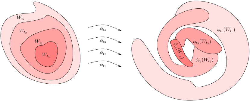
Figure 1. The figure illustrates the hypothesis of Theorem 4.3. Here $t_{1}<t_{2}<t_{3}<t_{4}$. The theorem does not say that the family of embeddings $(\phi_{t}\colon W_{t}\hookrightarrow M)_{t\in(0,\,a)}$ has a limit as $t\to 0$. Actually, the images $\phi_{t}(W_{t})$ may overlap in complicated ways, be disjoint etc. An embedding on the union of all the $W_{t}$ can be constructed using Hamiltonian flows to modify the family, see the proof of the result.

Remark 4.4. If $N=\mathbb{R}^{2n}$ and if there is a continuous function $r\colon(0,a)\subset\mathbb{R}\to(0,\infty)$, $v\mapsto r(v)$, such that $\phi_{v}(W_{v})$ is contained in ${\rm B}^{2d}(r(v))$ for every $v\in(0,a)$, then the hypothesis in Theorem 4.3 that for any fixed $t,s>0$, the set $\bigcup_{v\in[t,s]}\phi_{v}(W_{v})$ is relatively compact in $M$, is automatically satisfied. Indeed, we have that $\overline{\bigcup_{v\in[t,s]}\phi_{v}(W_{v})}\subset\overline{{\rm B}^{2d}(\max_{t\in[t,s]}r(v))}.$ $\oslash$

Key lemmas

We use two lemmas in order to prove Theorem 4.3.

Lemma 4.5.

Let $W_{t}\subset N$, $t\in(0,a)$, be a family of simply connected open subsets of a symplectic manifold $N$. Let $(\phi_{t}\colon W_{t}\hookrightarrow M)_{t\in(0,a)}$ be a smooth family of symplectic embeddings such that:

• $\overline{W_{s}}\subset W_{t}$ when $t<s$;

• for any $t,s>0$, the set $\bigcup_{v\in[t,s]}\phi_{v}(W_{v})$ is relatively compact in $M$.

Then for any $t<t^{\prime}<s$ there exists a smooth time-dependent Hamiltonian $G_{v}:M\to{\mathbb{R}}$, $v\in[t,t^{\prime}]$, whose Hamiltonian flow $\psi_{v}$ starting at $v=t$ is defined for all $v\in[t,t^{\prime}]$ and satisfies $\psi_{t^{\prime}}\circ\phi_{t}|_{W_{s}}=\phi_{t^{\prime}}|_{W_{s}}.$

Proof.

We divide the proof into three steps.

Step 1. Let $s^{\prime\prime}\in(t^{\prime},s)$. Let $x\in W_{s^{\prime\prime}}$. By (i) we have that for any $v\in[t,t^{\prime}]$, $x\in W_{v}$. Therefore one can take the following derivative :

$$X_{v}(\phi_{v}(x)):=\frac{\partial\phi_{v}(x)}{\partial v},$$

which defines a vector field on $\phi_{v}(W_{s^{\prime\prime}})$. Because all $\phi_{v}$’s are symplectic, the time-dependent vector field $X_{v}$ is symplectic. Hence the pull-back $(\phi_{v})^{*}X_{v}$ is symplectic. Since $W_{s^{\prime\prime}}$ is simply connected, $(\phi_{v})^{*}X_{v}|_{W_{s^{\prime\prime}}}$ is Hamiltonian : there exists a smooth function $(x,v)\mapsto\tilde{H}_{v}(x)$ on $W_{s^{\prime\prime}}\times[t,t^{\prime}]$ such that

$$\iota_{(\phi_{v})^{*}{X_{v}}}\omega=-\mathrm{d}\tilde{H}_{v}.$$

We let

$$H_{v}(y):=\tilde{H}_{v}(\phi_{v}^{-1}(y)),$$

which is a Hamiltonian function defined on $\phi_{v}(W_{s^{\prime\prime}})$ for the vector field $X_{v}$. This concludes Step 1.

Step 2. We’ll construct a smooth family $(\tau_{v}:M\to{\mathbb{R}})_{v\in[t,t^{\prime}]}$, with :

(1) $$\tau_{v}|_{\phi_{v}(W_{s})}\equiv 1;$$

(2) $$\tau_{v}|_{M\setminus\phi_{v}(W_{v})}\equiv 0.$$

In order to do this, fix $s^{\prime}\in(s^{\prime\prime},s)$, and let $\chi\in\textup{C}^{\infty}(M)$ be equal to $1$ on $W_{s}$ and to $0$ on $M\setminus W_{s^{\prime}}$. We simply define

$$\tau_{v}(y):=\begin{cases}\chi\circ\phi_{v}^{-1}(y)&\text{ if }y\in\phi_{v}(W_{v})\\ 0&\text{ otherwise.}\end{cases}$$

The map $\tau_{v}$, for $v\in[t,t^{\prime}]$, satisfies (1) and (2). It remains to see that $(v,y)\mapsto\tau_{v}(y)$ is smooth. First, let $(v_{0},y_{0})\in[t,t^{\prime}]\times M$ be such that $y_{0}\in\phi_{v_{0}}(W_{v_{0}})$. Using the continuity of the family $(\phi_{v})$ and the fact that $\phi_{v_{0}}(W_{v_{0}})$ is open in $M$, we see that $y\in\phi_{v}(W_{v})$ for $(v,y)$ in a small open neighborhood of $(v_{0},y_{0})$. Hence, in this neighborhood,

$$(v,y)\mapsto\tau_{v}(y)=\chi\circ\phi^{-1}(v)$$

is smooth. Second, suppose that $y_{0}\not\in\phi_{v_{0}}(W_{v_{0}})$. Therefore $y_{0}\not\in\phi_{v_{0}}(\overline{W_{s^{\prime}}})$, and the latter being closed, there is a small neighborhood of $(v_{0},y_{0})$ in which all $(v,y)$ satisfy $y\not\in\phi_{v}(\overline{W_{s^{\prime}}})$. Hence $y\not\in\phi_{v}(W_{s^{\prime}})$, and both cases in the definition of $\tau_{v}$ lead to $\tau_{v}(x)=0$, which proves the smoothness.

Step 3. We may now define a smooth time dependent Hamiltonian $G\colon[t,\,t^{\prime}]\times M\to\mathbb{R}$ by

$$G_{v}(y)=H_{v}(y)\tau_{v}(y)$$

for $y\in\phi_{v}(W_{v})$ and $G_{v}(y)=0$ for $y\in M\setminus\phi_{v}(W_{v})$. Of course, $G_{v}=H_{v}$ on $\phi_{v}(W_{s})$.

Let $Y_{v}$ be the Hamiltonian vector field associated to $G_{v}$ and let $\psi(v,y)$ be the flow of $Y_{v}$ starting from time $t$ :

$$\begin{cases}\displaystyle\frac{\partial\psi(v,y)}{\partial v}=Y_{v}(\psi(v,y))\\ \psi(t,y)=y.\end{cases}$$

The vector field $Y_{v}$ vanishes outside of the fixed set $\bigcup_{v\in[t,t^{\prime}]}\phi_{v}(W_{v}),$ which is relatively compact in $M$ for any fixed $t,t^{\prime}>0$ by assumption (ii). This implies that the flow $\psi(v,y)$ can be integrated up to time $t^{\prime}$.

Let

$$\varphi(v,x):=\psi(v,\phi_{t}(x)).$$

Then $\varphi$ satisfies the Cauchy problem on $W_{s}$ :

$$\begin{cases}\displaystyle\frac{\partial\varphi(v,x)}{\partial v}=Y_{v}(\varphi(v,x))=X_{v}(\varphi(v,x))\\ \varphi(t,x)=\phi_{t}(x).\end{cases}$$

Therefore, for all $x\in W_{s}$, $\varphi(v,x)=\phi_{v}(x).$ In particular, when $v=t^{\prime}$, we get, with $\Psi(y):=\psi(t^{\prime},y)$,

$$\Psi\circ\phi_{t}|_{W_{s}}=\phi_{t^{\prime}}|_{W_{s}}$$

This concludes the proof. ∎

Lemma 4.6.

Let $V_{1}\subset V_{2}\subset\ldots\subset V_{n}\subset\ldots$ be a sequence of simply connected open subsets of a symplectic manifold $N$. Let $i_{n}\colon V_{n}\hookrightarrow M$, $n\in\mathbb{N}^{*}$, be a sequence of symplectic embeddings into another symplectic manifold $M$ such that for any $n\geqslant 2$ there exists a symplectomorphism $\psi_{n}\colon M\to M$ satisfying

$$\psi_{n}\circ i_{n+1}|_{V_{n-1}}=i_{n}|_{V_{n-1}}.$$

Denote

$$V:=\bigcup_{n=1}^{\infty}V_{n}.$$

Then there exists a symplectic embedding $j\colon V\hookrightarrow M$.

Proof.

Define $j\colon V\to M$ by

$$j(x):=\psi_{2}\circ\psi_{3}\circ\ldots\circ\psi_{n-1}\circ i_{n}(x)$$

for $x\in V_{n-1}\subset V$ for $n>2$. This definition is independent of the choice of $n>2$ for which $x\in V_{n-1}$. Then $j$ is a local symplectomorphism which is injective (any two points $x,y$ are contained in a common $V_{n-1}$); thus it is a symplectic embedding. ∎

Proof of Theorem 4.3

Consider the sequence of domains $V_{n}:=W_{1/n}.$ For each $n\geqslant 3$, consider the family

$$\left\{W_{t}\,\,|\,\,t\in{\textstyle\left(\frac{1}{n+2},\frac{1}{n-2}\right)}\right\},$$

and the values $s=\frac{1}{n-1},\,\,\,\,\,t=\frac{1}{n+1}\,\,\,\,\,\textup{and}\,\,\,\,\,t^{\prime}=\frac{1}{n}.$ Then Lemma 4.5 gives us a symplectomorphism $\psi_{n}:M\to M$ such that

$$\psi_{n}\circ i_{n+1}|_{V_{n-1}}=i_{n}|_{V_{n-1}},$$

which is the assumption of Lemma 4.6. Since $\bigcup_{n\geqslant 3}V_{n}=\bigcup_{t\in(0,\,a)}W_{t},$ we get Theorem 4.3.

5. Guth’s Lemma for families

The following statement is a smooth family version (see Definition 4) of the Main Lemma in Guth [10, Section 2]. As before, $n\geqslant 3$.

Lemma 5.1.

Let $\Sigma$ be the symplectic torus $\mathbb{T}^{2}=\mathbb{R}^{2}/\mathbb{Z}^{2}$ of area $1$ minus the “origin” (i.e. minus the lattice ${\mathbb{Z}}^{2}$, $\Sigma=({\mathbb{R}}^{2}\setminus{\mathbb{Z}}^{2})/{\mathbb{Z}}^{2}$). There is a smooth family $(i_{R})_{R>1/3}$ of symplectic embeddings $i_{R}\colon{\rm B}^{2(n-1)}(R)\hookrightarrow\Sigma\times{\rm B}^{2(n-2)}(10R^{2}).$

In order to verify Lemma 5.1 we need to explain why the construction in [10] depends smoothly on the parameter $R\in(1/3,\infty)$. Checking this amounts to checking that the “choices” therein made depend smoothly on $R$ and $\epsilon$. Guth’s Lemma is valid for $R=1/3$, however we shall see that the family is not smooth at this value (there is a square root singularity).

Proof.

We may restrict to $n=3$ with a smaller constant : $\textup{B}^{4}(R)\hookrightarrow\Sigma\times\textup{B}^{2}(\sqrt{72}R^{2}).$ Indeed, on the left hand-side we use the natural embedding $\textup{B}^{2(n-1)}(R)\subset B^{2(n-3)}(R)\times\textup{B}^{4}(R)$, and on the right hand-side we use the natural embedding $\textup{B}^{2(n-3)}(R)\times\textup{B}^{2}(\sqrt{72}R^{2})\subset\textup{B}^{2(n-1)}(\sqrt{72R^{4}+R^{2}})$ and notice that $\sqrt{72R^{4}+R^{2}}\leqslant 10R^{2}$, in view of $R>1/3$. To check smoothness with respect to $R$ we need to write some explicit formulas for maps and domains which were not explicitly written in Guth’s paper. Then the smoothness with respect to $R$ as in Definition 4 becomes equivalent to the smoothness of the formulas. In terms of the notation in Definition 4, we let $B=\textup{B}^{4}(1)\subset N={\mathbb{R}}^{4}$, $P=(1/3,\infty)$, the map $g$ is just a scaling : $g(R,b)=R\cdot b$, $R\in P$, $b\in B$, and $M=\Sigma\times{\mathbb{R}}^{2}$. Guth’s proof has two steps. The first one, due to Polterovich, is to construct a linear symplectic embedding of $\textup{B}^{4}(R)$ into ${\mathbb{T}}^{2}\times\textup{B}^{2}(\sqrt{72}R^{2})$, when $R\geqslant 1/3$. The second step is to modify this embedding by a nonlinear symplectomorphism in order to avoid a point in ${\mathbb{T}}^{2}$. Both steps depend on the radius $R$, therefore we have to check the smooth dependence.

Step 1. We want a plane $V_{R}\subset\mathbb{R}^{4}$, depending smoothly on $R$, such that

(3) $$\int_{{\rm B}^{4}(R)\cap V_{R}}\omega=\frac{\pi}{9}.$$

It turns out that one can give an easy formula for this plane. For $t>0$, let $W_{t}:={\rm span}\{(1,0,0,0),\,e_{t}\}$ with $e_{t}:=(0,t,1-t,0)$. Let $\varphi_{t}\colon\mathbb{R}^{2}\to W_{t}$ be the linear parameterization given by $\varphi(u,v):=(u,tv,(1-t)v,0).$ We have that $\varphi_{t}^{*}\omega=t{\rm d}v\wedge{\rm d}u$. On the one hand,

$${\rm B}^{4}(R)\cap W_{t} = \Big{\{}(x_{1},y_{1},x_{2},y_{2})\in V_{t}\,\,|\,\,(x_{1})^{2}+(y_{1})^{2}+(x_{2})^{2}+(y_{2})^{2}\leqslant R^{2}\Big{\}}$$

$$= \varphi_{t}\left(\Big{\{}(u,v)\in{\mathbb{R}}^{2}\,|\,\frac{u^{2}}{R^{2}}+\frac{v^{2}}{\frac{R^{2}}{2t^{2}-2t+1}}\leqslant 1\Big{\}}\right),$$

which is the image of an ellipse of area $\pi ab$, where $a=R$, $b=\frac{R}{\sqrt{2t^{2}-2t+1}}$. Therefore

$$\int_{\varphi_{t}^{-1}(\textup{B}^{4}(R)\cap W_{t})}t{\rm d}v\wedge{\rm d}u=\frac{t\pi R^{2}}{\sqrt{2t^{2}-2t+1}}.$$

If $R>1/3$, the equation $\frac{tR^{2}}{\sqrt{2t^{2}-2t+1}}=\frac{1}{9}$ has two solutions, and one of them is a smooth positive function $(1/3,\infty)\ni t\mapsto R(t)$. Thus, we may let $V_{t}:=W_{R(t)},$ and we satisfy (3).

Now, let $(f_{1,R},f_{2,R})$ be an orthonormal basis of $V_{R}$, and $(f_{1,R}^{\perp},f_{2,R}^{\perp})$ be a symplectic basis of the symplectic orthogonal complement $V_{R}^{\perp}$. These basis may be chosen to depend smoothly on $R$. Then the linear map

$$(L_{R})^{-1}\colon(x_{1},y_{1},x_{2},y_{2})\mapsto\lambda x_{1}f_{1,R}+y_{1}f_{2,R}+x_{2}f_{1,R}^{\perp}+y_{2}f_{2,R}^{\perp}$$

is symplectic when $\omega(\lambda f_{1,R},f_{2,R})=1$, i.e. $\lambda=(\omega(f_{1,R},f_{2,R}))^{-1}.$ Thus $(L_{R})_{R>1/9}$ is a smooth family of linear symplectomorphisms that map planes parallel to $V_{R}$ to planes parallel to the $(x_{1},y_{1})$-plane, and maps disks parallel to $V_{R}$ to disks. Let $P$ be an affine plane parallel to the $(x_{1},y_{1})$-plane and let $\tilde{P}_{R}=L_{R}^{-1}(P)$. Then ${\rm B}^{4}(R)\cap\tilde{P}_{R}$ is a ball of radius $\leqslant R$ parallel to ${\rm B}^{4}(R)\cap V_{R}$. Therefore, since $\omega$ is invariant by translation, we have that $\int_{{\rm B}^{4}(R)\cap\tilde{P}_{R}}\omega\leqslant\int_{{\rm B}^{4}(R)\cap V_{R}}\omega=\frac{\pi}{9}.$ (note that ${\rm B}^{4}(R)\cap\tilde{P}_{R}$ can be translated to be a subset of ${\rm B}^{4}(R)\cap V_{R}$.) We know that $L_{R}({\rm B}^{4}(R)\cap\tilde{P}_{R})$ must be a Euclidean disk $\textup{B}^{2}(r)$ in the $(x_{1},y_{1})$-plane. Since $L_{R}$ is symplectic, we have that

$$\int_{L_{R}({\rm B}^{4}(R))\cap P}\omega=\int_{\underbrace{\scriptstyle L_{R}({\rm B}^{4}(R)\cap\tilde{P}_{R})}_{{\rm B}^{2}(r)}}\omega=\int_{{\rm B}^{4}(R)\cap\tilde{P}_{R}}\omega\leqslant\frac{\pi}{9},$$

and therefore $\int_{{\rm B}^{2}(r)}{\rm d}x_{1}\,{\rm d}y_{1}\leqslant\frac{\pi}{9},$ and hence $r\leqslant 1/3$. $L_{R}(\textup{B}^{4}(R))$ is an ellipsoid (by this we mean the open set bounded by the ellipsoid) in ${\mathbb{R}}^{4}$ whose half-axes are smooth, positive functions of $R$. Hence its projection onto the $(x_{2},y_{2})$-plane is an ellipse with the same properties. Therefore, there exists a smooth positive function $\mu(R)$ such that the projection onto the $(x_{2},y_{2})$-plane of $\ell_{R}\circ L_{R}(\textup{B}^{4}(R))$ is a disk, where $\ell_{R}$ is the symplectomorphism

$$(x_{1},y_{1},x_{2},y_{2})\mapsto(x_{1},y_{1},\mu(R)x_{2},(\mu(R))^{-1}y_{2}).$$

In the sequel, we assume that $L_{R}$ is this new symplectomorphism $\ell_{R}\circ L_{R}$.

The rest of the proof of Step 1 does not involve any construction depending on $R$. We repeat the argument here for the sake of completeness. Let $Q:{\mathbb{R}}^{2}\times{\mathbb{R}}^{2}\to{\mathbb{T}}^{2}\times{\mathbb{R}}^{2}$ be the map defined as the quotient map ${\mathbb{R}}^{2}\to{\mathbb{T}}^{2}$ on the first factor, and the identity on the second one (see Figure 2).

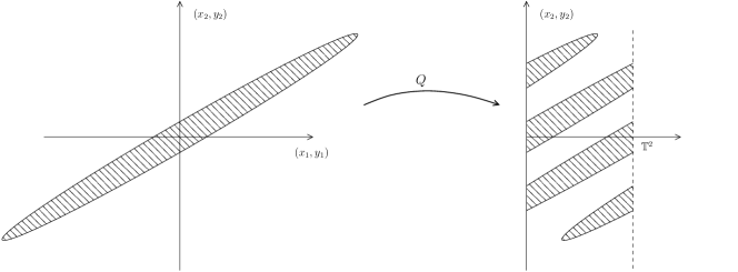
Figure 2. Vertical slices of the ellipsoid.

$Q$ restricted to the ellipsoid $L_{R}(\textup{B}^{4}(R))$ is injective : indeed the “vertical” coordinates $(x_{2},y_{2})$ are preserved, and the intersection of $L_{R}(\textup{B}^{4}(R))$ with a horizontal plane is a disk of radius $\leqslant\frac{1}{3}<\frac{1}{2}$. Hence $Q|_{L_{R}(\textup{B}^{4}(R))}$ is an embedding. The desired embedding is $Q\circ L_{R}$, which depends smoothly on $R$. Let $\pi_{2}:{\mathbb{R}}^{2}\times{\mathbb{R}}^{2}\to{\mathbb{R}}^{2}$ be the projection onto the second factor. It remains to estimate the size of $\pi_{2}(L_{R}(\textup{B}^{4}(R)))$, which we know is an open disk. Let $S$ be the radius of this disk, and let $p=(x_{2},y_{2})$ be a point in the concentric disk of radius $S/2$. Because of (3), the preimage $\pi_{2}^{-1}(0,0)$ is a disk of radius $1/3$. Since the ellipsoid is convex, the preimage $\pi_{2}^{-1}(p)$ (which is a disk) must have a radius at least $1/6$. We can now get a lower bound for the volume $v$ of $L_{R}(\textup{B}^{4}(R))$ by integrating over the subset which projects onto $x_{2}^{2}+y_{2}^{2}\leqslant S^{2}/4$ : $v\geqslant\pi\frac{S^{2}}{4}\frac{\pi}{36}$. Since $L_{R}$ is symplectic and hence volume preserving, $v$ is also the volume of $\textup{B}^{4}(R)$ : $v=\frac{1}{2}\pi^{2}R^{4}$. Hence $S\leqslant\sqrt{72}R^{2}$.

Step 2. We want now to modify $L_{R}$ by a nonlinear symplectomorphism $\tilde{\Psi}_{R}$, such that the image $\tilde{\Psi}_{R}\circ L_{R}(\textup{B}^{4}(R))$ avoids the integer lattice ${\mathbb{Z}}^{2}\times{\mathbb{R}}^{2}$. Then the required embedding will simply be $Q\circ\tilde{\Psi}_{R}\circ L_{R}$.

We are not going to repeat Guth’s argument, but simply to point out the smooth dependence on $R$. Let $\pi_{1}:{\mathbb{R}}^{2}\times{\mathbb{R}}^{2}\to{\mathbb{R}}^{2}$ be the projection onto the first factor. Let $\rho(R)\geqslant 1$ be a smooth function such that the ellipse $\pi_{1}(L_{R}(\textup{B}^{4}(R)))$ is contained in the disk of radius $\rho(R)$. For instance one can take $\rho(R)$ to be $1$ plus the sum of the two half-axes of the ellipse. Then $\tilde{\Psi}_{R}=\Psi_{R}\otimes\textup{Id}_{{\mathbb{R}}}$, where $\Psi_{R}$ is a symplectomorphism of ${\mathbb{R}}^{2}$, obtained by lifting a diffeomorphism $\Phi_{R}$ of the $x_{1}$ variable. We define $\Phi_{R}(x_{1})=x_{1}+f_{R}(x_{1}),$ where $f_{R}\colon\mathbb{R}\to\mathbb{R}$ is a smooth function that satisfies the following properties :

1. $f^{\prime}_{R}(x_{1})\geqslant-0.1$;

2. $f_{R}$ is periodic of period $1$;

3. $f_{R}(k)=0$, $\forall k\in{\mathbb{Z}}$;

4. $f^{\prime}_{R}(k)=100\rho(R)$, $\forall k\in{\mathbb{Z}}$;

5. $\left|f_{R}\right|\leqslant 10^{-4}$;

6. The map $(1/3,\infty)\times{\mathbb{R}}\ni(R,x_{1})\mapsto f_{R}(x_{1})$ is smooth.

A function satisfying these requirements is depicted in Figure 3. ∎

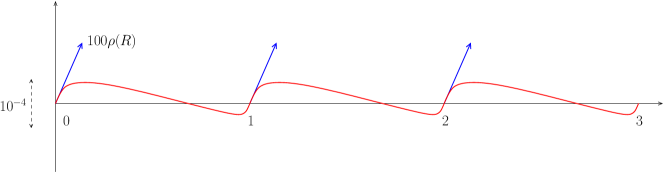
Figure 3. function $f_{R}$.

6. Embeddings into ${\rm B}^{2}(R)\times{\rm B}^{2}(R)\times\mathbb{R}^{2(n-2)}$

We start with a particular case of the classical non-compact Moser theorem (see also [25, Theorem B.1, Appendix]):

Lemma 6.1 (Greene and Shiohama, Theorem 1 in [7]).

If $\Sigma$ is a connected oriented $2$-manifold and if $\omega$ and $\tau$ are area forms on $\Sigma$ which give the same finite area, then there is a symplectomorphism $\varphi\colon(\Sigma,\omega)\to(\Sigma,\tau)$.

The Greene-Shiohama result remains valid when varying with respect to smooth parameters.

Lemma 6.2.

Let $I\subset\mathbb{R}$ be an interval. Let $\{M_{\delta}\}_{\delta\in I}$ and $\{N_{\delta}\}_{\delta\in I}$ be smooth families of connected $2$-manifolds such that on each $M_{\delta},N_{\delta}$ there are area forms $\omega_{\delta},\tau_{\delta}$, respectively, giving the same finite area for each $\delta\in I$. Then there is a smooth family of symplectomorphisms $(\varphi_{\delta}\colon M_{\delta}\to N_{\delta})_{\delta\in I}$.

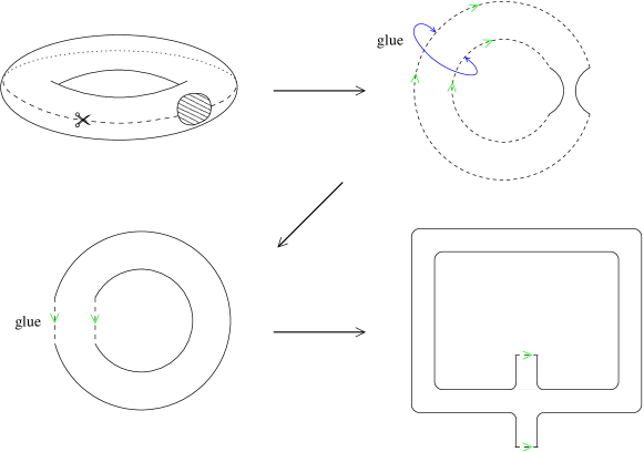
Figure 4. Steps to arrive at Figure 5.

The following is a smooth family version of the main statement proven by Hind and Kerman in [11, Section 4.1]. It concerns ball embeddings constructed using Hamiltonian flows. As before, let $\Sigma$ be the symplectic torus $\mathbb{T}^{2}=\mathbb{R}^{2}/\mathbb{Z}^{2}$ of area $1$ minus the “origin” (i.e. minus the lattice ${\mathbb{Z}}^{2}$).

Theorem 6.3.

For any $\epsilon>0$, we let $\Sigma(\epsilon):=({\mathbb{R}}^{2}\setminus\sqrt{\epsilon}{\mathbb{Z}}^{2})/\sqrt{\epsilon}{\mathbb{Z}}^{2}$ be the scaling of $\Sigma$ with symplectic area $\epsilon$. There exist constants $\epsilon_{0}>0$, $c>0$, and a smooth family $({I}_{\epsilon})_{\epsilon\in(0,\epsilon_{0}]}$ of symplectic embeddings ${I}_{\epsilon}\colon\Sigma(\epsilon)\times{\rm B}^{2}(1)\hookrightarrow{\rm B}^{2}(\sqrt{2}+c\epsilon)\times{\rm B}^{2}(\sqrt{2}).$

Proof.

We have organized the proof in several steps. As in the proof of Lemma 5.1, smoothness is the sense of Definition 4.

Step 1 (Definition of immersion $i_{\epsilon}$). For sufficiently small fixed $\epsilon>0$ we may define a smooth immersion

(4) $$i_{\epsilon}\colon\Sigma(\tilde{\epsilon})\hookrightarrow\mathbb{R}^{2},$$

where

(5) $$\tilde{\epsilon}:=100\epsilon$$

by Figure 5, with $a=\epsilon^{2}$. In particular, the double points of the immersion are concentrated in the small region $[-a,a]\times[-\epsilon/2,\epsilon/2]$. The topological steps to transform the punctured torus $\Sigma(\tilde{\epsilon})$ into such a domain are depicted in Figure 4.

Step 2 (Modifying $i_{\epsilon}$ to make it symplectic). By Moser’s argument applied to $(\Sigma(\tilde{\epsilon}),\omega_{\Sigma(\tilde{\epsilon})})$ and $(\Sigma(\tilde{\epsilon}),i_{\epsilon}^{*}\omega_{0})$ (Lemma 6.2), where $\omega_{0}$ is the standard symplectic form on $\mathbb{R}^{2}$, the immersion (4) may be modified so as to obtain a symplectic immersion. For this to hold, we need that

(6) $$\int_{\Sigma(\tilde{\epsilon})}i_{\epsilon}^{*}\omega_{0}={\rm area\,\,of}\,\,\Sigma(\tilde{\epsilon}).$$

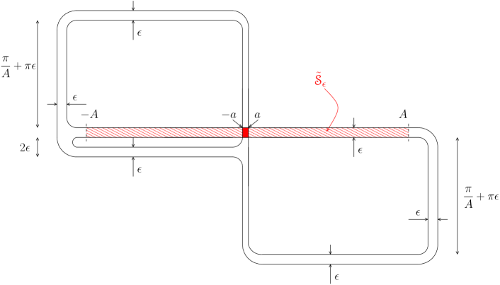
Figure 5. The immersion $i_{\epsilon}\colon\Sigma(\tilde{\epsilon})\hookrightarrow\mathbb{R}^{2}$.

The right hand side of (6) is equal to $\tilde{\epsilon}=100\epsilon$ by definition of $\Sigma(\tilde{\epsilon})$. Let’s compute the left hand side of (6). From Figure 5, it is equal, for sufficiently small $\epsilon>0$, to the sum of the areas of five horizontal rectangles of area $A\epsilon$, and four vertical rectangles of area $\frac{\pi\epsilon}{A-a}$, plus several corner squares whose area is a smooth function of $\epsilon$ of order $\epsilon^{2}$. Since $a=\epsilon^{2}$ we obtain that, for sufficiently small $\epsilon>0$ :

(7) $$\int_{\Sigma(\tilde{\epsilon})}i_{\epsilon}^{*}\omega_{0}=5A\epsilon+\frac{4\pi\epsilon}{A}+\mathcal{O}(\epsilon^{2}).$$

Let $p(A)=\int_{\Sigma(\tilde{\epsilon})}i_{\epsilon}^{*}\omega_{0}$, so that (6) is equivalent to $p(A)=100\epsilon$. We need to show that this equation has at least one solution which should be bounded from below by a positive constant independent of $\epsilon$. This follows from the study of the second order equation $q(A)=0$, where $q(A):=A(p(A)/\epsilon-100)=5A^{2}+(\mathcal{O}(\epsilon)-100)A+4\pi$, which has two positive solutions $A\geqslant\frac{1}{8}$ provided that we chose $\epsilon$ in Step 1 to be small enough. Hence by choosing $A=A(\tilde{\epsilon})$ to be either solution we have a smoothly dependent function on $\tilde{\epsilon}$ for which Moser’s equation (6) holds. Therefore we may apply the non-compact Moser theorem (Lemma 6.2) to get a diffeomorphism $\varphi_{\epsilon}\colon\Sigma(\tilde{\epsilon})\to\Sigma(\tilde{\epsilon})$ such that $\varphi_{\epsilon}^{*}(i_{\epsilon}^{*}\omega_{0})=\omega_{\Sigma(\tilde{\epsilon})}$ and therefore by composing $i_{\epsilon}$ with $\varphi_{\epsilon}$ we may assume that (4) is symplectic. This concludes Step 2.

Step 3 (Preparatory cut-off functions). Choose a smooth cut-off function $\chi_{\epsilon}\colon\mathbb{R}\to[0,1]$ which is non decreasing on ${\mathbb{R}}^{-}$, non increasing on ${\mathbb{R}}^{+}$, taking values as follows :

(8) $$\chi_{\epsilon}\equiv 1 \,\,\,\,\,\,[-a,\,a];$$ on

(9) $$\chi_{\epsilon}\equiv 0 \,\,\,\,\,\,\mathbb{R}\setminus[-A+\epsilon^{2},\,A-\epsilon^{2}],$$ on

and such that it satisfies the following bounds :

• For every $x\in\mathbb{R}$,

  (10) $$|\chi^{\prime}_{\epsilon}(x)|\leqslant\frac{1}{A}+\epsilon.$$

• For every $x\in[-A+\frac{\epsilon}{2},\,A-\frac{\epsilon}{2}]$,

  (11) $$\biggl{\rvert}\chi_{\epsilon}(x)-\Big{(}1-\frac{|x|}{A}\Big{)}\biggr{\rvert}\leqslant\epsilon.$$

Such a function $\chi_{\epsilon}$ is depicted in Figure 6. The ${\rm C}^{0}$ estimate (11) follows from $d=\frac{\epsilon}{200A}\leqslant\epsilon$ (recall that $A\geqslant\frac{1}{8}$). The ${\rm C}^{1}$ estimate (10) follows from the fact that the maximum slope of the graph in Figure 6 is $\dfrac{1}{A-\frac{\epsilon}{100}}$ and that, when $\epsilon<A$,

$$\frac{1}{A-\tfrac{\epsilon}{100}}\leqslant\frac{1}{A}+\epsilon.$$

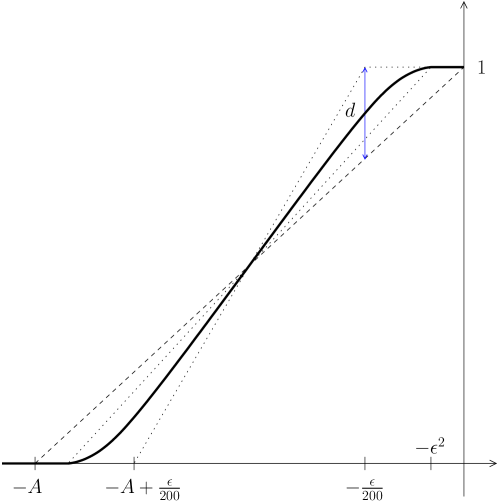
Figure 6. The cut-off function $\chi_{\epsilon}$. We have represented the $x<0$ part; the function is symmetric with respect to $x=0$.

This concludes Step 3.

Step 4 (The smooth map $\mathcal{I}_{\epsilon}$). On $\mathbb{R}^{2}\times\mathbb{R}^{2}$ we define the smooth family of Hamiltonian functions $(\mathcal{H}_{\epsilon}(x_{1},y_{1},x_{2},y_{2}):=-\chi_{\epsilon}(x_{1})x_{2}\,\sqrt{\pi})_{\epsilon}$ whose time-$1$ flows are given by the smooth family $(\Phi_{\epsilon})_{\epsilon}$ :

(12) $$\,\,\,\,\,\,\,\,\,\,\Phi_{\epsilon}(x_{1},y_{1},x_{2},y_{2})=\Big{(}x_{1},\,\,y_{1}+\chi^{\prime}_{\epsilon}(x_{1})x_{2}\sqrt{\pi},\,\,x_{2},\,\,y_{2}+\chi_{\epsilon}(x_{1})\sqrt{\pi}\Big{)}.$$

Let ${\rm Q}(\sqrt{\pi})$ denotes the open square $(0,\sqrt{\pi})\times(0,\sqrt{\pi})$ and ${\rm R}(\sqrt{\pi},2\sqrt{\pi})$ be the open rectangle $(0,\sqrt{\pi})\times(0,2\sqrt{\pi})$. Let $\mathcal{S}_{\epsilon}$ be the connected subset of $\Sigma(\tilde{\epsilon})$ that is mapped to the horizontal strip $\widetilde{\mathcal{S}_{\epsilon}}=(-A,A)\times(-\frac{\epsilon}{2},\frac{\epsilon}{2})$ by the immersion $i_{\epsilon}$ (See Figure 5). We define $\mathcal{I}_{\epsilon}\colon\Sigma(\tilde{\epsilon})\times{\rm Q}(\sqrt{\pi})\to\mathbb{R}^{4}$ by

(13) $$\mathcal{I}_{\epsilon}(\sigma,\,b):=\begin{cases}\Phi_{\epsilon}(i_{\epsilon}(\sigma),b)&\text{ if }\sigma\in\mathcal{S}_{\epsilon};\\ (i_{\epsilon}(\sigma),b)&\text{ if }\sigma\notin\mathcal{S}_{\epsilon}.\\ \end{cases}$$

Since $0\leqslant\chi_{\epsilon}\leqslant 1$, the image of $\mathcal{I}_{\epsilon}$ lies in the set $\mathbb{R}^{2}\times{\rm R}(\sqrt{\pi},2\sqrt{\pi})$. Moreover, $\mathcal{I}_{\epsilon}$ is smooth because the Hamiltonian flow $\Phi_{\epsilon}$ in (12) is the identity near $x=\pm A$, $y\in(-\frac{\epsilon}{2},\frac{\epsilon}{2})$ (since $\chi_{\epsilon}=0$ there by (9)). For the same reason, $\mathcal{I}_{\epsilon}$ is a local diffeomorphism, since $i_{\epsilon}$ is a local diffeomorphism and $\Phi_{\epsilon}$ is a diffeomorphism.

Step 5 ($\mathcal{I}_{\epsilon}$ is injective). Assume $\mathcal{I}_{\epsilon}(\sigma,b)=\mathcal{I}_{\epsilon}(\sigma^{\prime},b^{\prime})$. There are three cases.

• Suppose that $\sigma\in\mathcal{S}_{\epsilon}$ and $\sigma^{\prime}\in\mathcal{S}_{\epsilon}$. Then $\Phi_{\epsilon}(i_{\epsilon}(\sigma),b)=\Phi_{\epsilon}(i_{\epsilon}(\sigma^{\prime}),b^{\prime}),$ so since $\Phi_{\epsilon}$ is a diffeomorphism, $(i_{\epsilon}(\sigma),b)=(i_{\epsilon}(\sigma^{\prime}),b^{\prime})$. Since $i_{\epsilon}|_{\mathcal{S}_{\epsilon}}$ is injective, we have that $\sigma=\sigma^{\prime}$ and $b=b^{\prime}$ as we wanted.

• Suppose that $\sigma\notin\mathcal{S}_{\epsilon}$ and $\sigma^{\prime}\notin\mathcal{S}_{\epsilon}$. Then $(i_{\epsilon}(\sigma),b)=(i_{\epsilon}(\sigma^{\prime}),b^{\prime})$ and since $i_{\epsilon}$ is injective outside of $\mathcal{S}_{\epsilon}$, we have $\sigma=\sigma^{\prime}$ and $b=b^{\prime}$.

• Suppose that $\sigma\in\mathcal{S}_{\epsilon}$ and $\sigma^{\prime}\notin\mathcal{S}_{\epsilon}$. We have that $\Phi_{\epsilon}(i_{\epsilon}(\sigma),b)=(i_{\epsilon}(\sigma^{\prime}),b^{\prime}).$ Let us write in coordinates $(x_{1},y_{1},x_{2},y_{2})=(i_{\epsilon}(\sigma),b)$ and $(x^{\prime}_{1},y^{\prime}_{1},x^{\prime}_{2},y^{\prime}_{2})=(i_{\epsilon}(\sigma^{\prime}),b^{\prime})$. From (12) we have

  (14) $$\begin{cases}x^{\prime}_{1}=x_{1};\\ x^{\prime}_{2}=x_{2};\\ y^{\prime}_{1}=y_{1}+\chi_{\epsilon}^{\prime}(x_{1})x_{2}\sqrt{\pi};\\ y^{\prime}_{2}=y_{2}+\chi_{\epsilon}(x_{1})\sqrt{\pi}.\\ \end{cases}$$

  In particular, $|y^{\prime}_{2}-y_{2}|=\chi_{\epsilon}(x_{1})\sqrt{\pi}.$ Since $y_{2}\in(0,\sqrt{\pi})$ and $y^{\prime}_{2}\in(0,\sqrt{\pi})$ we must have that $\chi_{\epsilon}(1)<1$. Hence $|x_{1}|>a$, and we are outside of the vertical strip $|x_{1}|\leqslant a$. If $x_{1}<-a$, the second to last equation in (14), and the slope bound (10), imply

  (15) $$\begin{cases}y_{1}\leqslant y^{\prime}_{1}<y_{1}+\bigl{(}\frac{1}{A}+\epsilon\bigr{)}\pi;\\ x_{1}\geqslant-A\,\,\,\,\,\,(\textup{because}\,\,\,\sigma\in\mathcal{S}_{\epsilon}).\end{cases}$$

  It follows from Figure 5 that (15) is not possible.

  Similarly, if $x_{1}>a$ then $\chi^{\prime}\leqslant 0$, and we have that $y_{1}\geqslant y^{\prime}_{1}>y_{1}-\bigl{(}\frac{1}{A}+\epsilon\bigr{)}\pi,$ which is, again by Figure 5, impossible.

This concludes Step 5.

Step 6 (Conclusion). We have so far shown that we have a smooth embedding

(16) $$\mathcal{I}_{\epsilon}\colon\Sigma(\tilde{\epsilon})\times{\rm Q}(\sqrt{\pi})\to\mathbb{R}^{2}\times{\rm R}(\sqrt{\pi},\,2\sqrt{\pi})$$

for sufficiently small values of $\epsilon>0$. From the formula (12) for the flow $\Phi_{\epsilon}$ we have that $\pi_{1}(\mathcal{I}_{\epsilon}(\Sigma(\tilde{\epsilon})\times{\rm Q}(\sqrt{\pi})))\subset D_{\epsilon},$ where $D_{\epsilon}$ is depicted in Figure 7, and $\pi_{1}\colon\mathbb{R}^{2}\times\mathbb{R}^{2}\to\mathbb{R}^{2}$ is the projection onto the first factor. So $\mathcal{I}_{\epsilon}$ gives an embedding

(17) $$\mathcal{I}_{\epsilon}\colon\Sigma(\tilde{\epsilon})\times{\rm Q}(\sqrt{\pi})\hookrightarrow D_{\epsilon}\times{\rm R}(\sqrt{\pi},\,2\sqrt{\pi}).$$

Let $(\varphi_{\epsilon}\colon D_{\epsilon}\hookrightarrow{\rm B}^{2}(r(\epsilon)))_{\epsilon>0}$ be a smooth family of symplectic embeddings, where

(18) $$r(\epsilon)=\sqrt{\frac{{\rm Area}(D_{\epsilon})}{\pi}}.$$

Such family exists by Moser’s argument (Lemma 6.2). By construction of $D_{\epsilon}$ (Figure 7) there exists a constant $\tilde{c}>0$ such that $r(\epsilon)\leqslant\sqrt{2}+\tilde{c}\epsilon$, for sufficiently small $\epsilon>0$. Again by Moser’s argument there are symplectomorphisms

(19) $$f\colon{\rm R}(\sqrt{\pi},\,2\sqrt{\pi})\to{\rm B}^{2}(\sqrt{2})$$

and

(20) $$g\colon{\rm B}^{2}(1)\to{\rm Q}(\sqrt{\pi}).$$

We may combine the maps (17), (19), and (20) to get a smooth family of symplectic embeddings $(I_{\tilde{\epsilon}})_{\tilde{\epsilon}>0}$, for $\tilde{\epsilon}$ sufficiently small, defined as follows

$$\Sigma(\tilde{\epsilon})\times{\rm B}^{2}(1)\stackrel{{\scriptstyle{\rm Id}\otimes g}}{{\hookrightarrow}}\Sigma(\tilde{\epsilon})\times{\rm Q}(\sqrt{\pi})\stackrel{{\scriptstyle\mathcal{I}_{\epsilon}}}{{\hookrightarrow}}D_{\epsilon}\times{\rm R}(\sqrt{\pi},2\sqrt{\pi})$$

$$\stackrel{{\scriptstyle{\rm Id}\otimes f}}{{\hookrightarrow}}D_{\epsilon}\times{\rm B}^{2}(\sqrt{2})\stackrel{{\scriptstyle\varphi_{\epsilon}\otimes{\rm Id}}}{{\hookrightarrow}}{\rm B}^{2}(\sqrt{2}+c\tilde{\epsilon})\times{\rm B}^{2}(\sqrt{2}),$$

where $c=\tilde{c}/100$. This concludes the proof.∎

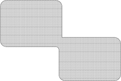
Figure 7. The open set $D_{\epsilon}$ is the envelope of the image of the immersion $i_{\epsilon}$ in Figure 5. Hence the total area of $D_{\epsilon}$ is of order $2(\tfrac{\pi}{A}\times A)+\mathcal{O}(\epsilon)=2\pi+\mathcal{O}(\epsilon)$.

Next we prove that [11, Theorem 1.6] holds for smooth families.

Theorem 6.4.

Let $n\geqslant 3$. There exist constant $C,C^{\prime}>0$ and a smooth family of symplectic embeddings

$$i_{S,\,R}\colon{\rm B}^{2}(1)\times{\rm B}^{2(n-1)}(S)\hookrightarrow{\rm B}^{2}(R)\times{\rm B}^{2}(\sqrt{2})\times\textup{B}^{2(n-2)}({\textstyle\frac{CS^{2}}{\sqrt{R-\sqrt{2}}}}),$$

where $(S,R)$ vary in the open set

(21) $$\{(S,R)\in{\mathbb{R}}^{2}\,|\qquad S>0,\quad\sqrt{2}<R<\sqrt{2}+C^{\prime}S^{2}\}.$$

Proof.

Consider the symplectic embedding

$$i_{T}\colon{\rm B}^{2(n-1)}(T)\hookrightarrow\Sigma\times{\rm B}^{2(n-2)}(10T^{2}),\qquad T>{\textstyle\frac{1}{3}}$$

given by Lemma 5.1, where $\Sigma=({\mathbb{R}}^{2}\setminus{\mathbb{Z}}^{2})/{\mathbb{Z}}^{2}$ is equipped with the standard quotient symplectic form. For $\epsilon>0$, let $\tau_{\sqrt{\epsilon}}:{\mathbb{R}}^{2(n-1)}\to{\mathbb{R}}^{2(n-1)}$ be the dilation $\tau_{\sqrt{\epsilon}}(x)=\sqrt{\epsilon}x$. The corresponding quotient map $\bar{\tau}_{\sqrt{\epsilon}}$ maps $\Sigma\times{\mathbb{R}}^{2(n-2)}$ to $\Sigma(\epsilon)\times{\mathbb{R}}^{2(n-2)}$.

The map $\bar{\tau}_{\sqrt{\epsilon}}\circ i_{T}\circ(\tau_{\sqrt{\epsilon}})^{-1}$ is a symplectic embedding of $\tau_{\sqrt{\epsilon}}({\rm B}^{2(n-1)}(T))={\rm B}^{2(n-1)}(\sqrt{\epsilon}T)$ into

$$\bar{\tau}_{\sqrt{\epsilon}}(\Sigma\times{\rm B}^{2(n-2)}(10T^{2}))=\Sigma(\epsilon)\times{\rm B}^{2(n-2)}(10\sqrt{\epsilon}T^{2})).$$

Of course, as $T>\frac{1}{3}$ and $\epsilon>0$ vary, the corresponding family of embeddings is smooth. By composing with the embeddings given by Theorem 6.3, we obtain a smooth family of symplectic embeddings :

$${\rm B}^{2}(1)\times{\rm B}^{2(n-1)}(\sqrt{\epsilon}T)\hookrightarrow{\rm B}^{2}(\sqrt{2}+c\epsilon)\times{\rm B}^{2}(\sqrt{2})\times\textup{B}^{2(n-2)}(10\sqrt{\epsilon}T^{2}),$$

$$T>1/3,\quad\epsilon>0.$$

The conclusion of the theorem is obtained by the smooth change of parameters $(S,R):=(\sqrt{\epsilon}T,\sqrt{2}+c\epsilon)$, whose image is the domain given by (21), with $C^{\prime}=9c$. This change gives the constant $C=10\sqrt{c}$. ∎

7. Proof of Theorem 3.3

Hind and Kerman proved [11, Theorem 1.5] that for any $0<R_{1}<\sqrt{2}$ and any $R_{2}\geqslant R_{1}$ there are no symplectic embeddings of ${\rm B}^{2}(1)\times{\rm B}^{2(n-1)}(S)$ into ${\rm B}^{2}(R_{1})\times{\rm B}^{2}(R_{2})\times\mathbb{R}^{2(n-2)}$ when $S$ is sufficiently large. Therefore, in order to prove Theorem 3.3, it is sufficient to show that ${\rm B}^{2}(1)\times{\mathbb{R}}^{2(n-1)}$ symplectically embeds into ${\rm B}^{2}(\sqrt{2})\times{\rm B}^{2}(\sqrt{2})\times\mathbb{R}^{2(n-2)}$.

By Theorem 6.4 there exist constants $C,C^{\prime}>0$ and a smooth family of symplectic embeddings $i_{S,\,R}\colon{\rm B}^{2}(1)\times{\rm B}^{2(n-1)}(S)\hookrightarrow{\rm B}^{2}(R)\times{\rm B}^{2}(\sqrt{2})\times\textup{B}^{2(n-2)}({\textstyle\frac{CS^{2}}{\sqrt{R-\sqrt{2}}}}),$ where $(S,R)$ vary in the set $A$ of points $(S,R)\in{\mathbb{R}}^{2}$ such that $S>0$ and $\sqrt{2}<R<\sqrt{2}+C^{\prime}S^{2}$. Let $j_{R,S}$ be the symplectic rescaling :

$${\rm B}^{2}(\sqrt{2}/R)\times{\rm B}^{2(n-1)}(\sqrt{2}S/R)\hookrightarrow{\rm B}^{2}(\sqrt{2})\times{\rm B}^{2}(2/R)\times\textup{B}^{2(n-2)}({\textstyle\frac{C\sqrt{2}S^{2}}{R\sqrt{R-\sqrt{2}}}}),$$

given by $x\mapsto\sqrt{2}/R\,\,i_{S,R}(Rx/\sqrt{2})$. The family $(j_{R,S})_{(R,S)\in A}$ is again a smooth family of symplectic embeddings.

Consider the smooth subfamily

(22) $$\phi_{\epsilon}:=j_{S,R},\,\,\,\,\textup{with}\,\,\,\,\,S:=\frac{1}{\epsilon(1-\epsilon)},\,\,\,\,\,\,\,\,\,\,\,R:=\frac{\sqrt{2}}{1-\epsilon}.$$

A computation shows that $(R,S)\in A$ as long as

$$\epsilon^{3}(1-\epsilon)<\frac{C^{\prime}}{\sqrt{2}},$$

which holds if $\epsilon<\epsilon_{0}$ and $\epsilon_{0}<1$ is small enough; hence the family (22) is well defined, gives symplectic embeddings from ${\rm B}^{2}(1-\epsilon)\times{\rm B}^{2(n-1)}(1/\epsilon)$ to ${\rm B}^{2}(\sqrt{2})\times{\rm B}^{2}(\sqrt{2}(1-\epsilon))\times\textup{B}^{2(n-2)}(\rho(\epsilon))$ with

$$\rho(\epsilon):=\frac{2^{-1/4}C}{\sqrt{\epsilon^{5}(1-\epsilon)}}.$$

Of course, such a function $\rho\colon(0,\epsilon_{0})\to(0,\infty)$ is continuous and

$$\phi_{\epsilon}\left({\rm B}^{2}(1-\epsilon)\times{\rm B}^{2(n-1)}(1/\epsilon)\right) \subset{\rm B}^{2}(\sqrt{2})\times{\rm B}^{2}(\sqrt{2})\times\textup{B}^{2(n-2)}(\rho(\epsilon))$$

$$\subset{\rm B}^{2n}(2\sqrt{2}+\rho(\epsilon)).$$

Thus, in view of Remark 1 we may apply Theorem 4.3 to the family of symplectic embeddings (22) with target manifold $M={\rm B}^{2}(\sqrt{2})\times{\rm B}^{2}(\sqrt{2})\times{\mathbb{R}}^{2(n-2)}$ as in Definition 4. In this way we get a symplectic embedding $j\colon{\rm B}^{2}(1)\times{\mathbb{R}}^{2(n-1)}\hookrightarrow{\rm B}^{2}(\sqrt{2})\times{\rm B}^{2}(\sqrt{2})\times\mathbb{R}^{2(n-2)},$ as desired, thus proving Theorem 3.3.

Acknowledgements. We are thankful to Lev Buhovski for many fruitful discussions which have been important for the paper. We thank also Leonid Polterovich for helpful discussions concerning Moser’s theorem. We thank Helmut Hofer for helpful comments on the introduction to the paper. AP learned of the problem treated in this paper in a lecture by Helmut Hofer in the Winter of 2011 at Princeton University, and he is grateful to him for fruitful discussions and encouragement. AP was partly supported by NSF Grant DMS-0635607 and an NSF CAREER Award. VNS is partially supported by the Institut Universitaire de France, the Lebesgue Center (ANR Labex LEBESGUE), and the ANR NOSEVOL grant. He gratefully acknowledges the hospitality of the IAS.

Álvaro Pelayo
School of Mathematics
Institute for Advanced Study
Einstein Drive, Princeton, NJ 08540 USA

Washington University, Mathematics Department
One Brookings Drive, Campus Box 1146
St Louis, MO 63130-4899, USA.
E-mail: apelayo@math.wustl.edu
E-mail: apelayo@math.ias.edu

San Vũ Ngọc
Institut Universitaire de France

Institut de Recherches Mathématiques de Rennes
Université de Rennes 1, Campus de Beaulieu
F-35042 Rennes cedex, France
E-mail: san.vu-ngoc@univ-rennes1.fr

References

• [1] P. Biran: A stability property of symplectic packing, Invent. Math. 136 (1999)123-155.
• [2] P. Biran: Connectedness of spaces of symplectic embeddings, Int. Math. Res. Lett., 10 (1996) 487–491.
• [3] P. Biran: From symplectic packing to algebraic geometry and back, Proc. 3rd Europ. Congr. of Math., Barcelona 2, Prog. Math., Birkhauser (2001) 507–524.
• [4] K. Cieliebak, H. Hofer, J. Latschev, and F. Schlenk: Quantitative symplectic geometry. Dynamics, ergodic theory, and geometry, 1-44, Math. Sci. Res. Inst. Publ., 54, Cambridge Univ. Press, Cambridge, 2007.
• [5] I. Ekeland and H. Hofer: Symplectic topology and Hamiltonian dynamics. Math. Z. 200 (1989) 355–378.
• [6] A. Floer, H. Hofer, and K. Wysocki: Applications of symplectic homology. I. Math. Z. 217 (1994) 577-606.
• [7] R.E. Greene and S. Shiohama: Diffeomorphisms and volume-preserving embeddings of noncompact manifolds. Trans. Amer. Math. Soc. 255 (1979) 403-414.
• [8] M. Gromov: Partial Differential Relations. Springer-Verlag, Berlin, 1986. x+363 pp.
• [9] M. Gromov: Pseudoholomorphic curves in symplectic geometry, Invent. Math. 82 (1985) 307–347.
• [10] L. Guth: Symplectic embeddings of polydisks. Invent. Math. 172 (2008) 477–489.
• [11] R. Hind and E. Kerman: New obstructions to symplectic embeddings. arXiv:0906.4296v2.
• [12] H. Hofer: Symplectic capacities. In: Geometry of Low-dimensional Manifolds 2 (Durham, 1989). Lond. Math. Soc. Lect. Note Ser., vol. 151, pp. 15–34. Cambridge Univ. Press, Cambridge (1990).
• [13] H. Hofer: Symplectic invariants. Proceedings of the International Congress of Mathematicians, Vol. I, II (Kyoto, 1990), 521-528, Math. Soc. Japan, Tokyo, 1991.
• [14] H. Hofer and E. Zehnder: Symplectic Invariants and Hamiltonian Dynamics, Birkhäuser, Basel (1994).
• [15] M. Hutchings: Recent progress on symplectic embedding problems in four dimensions. Proc. Natl. Acad. Sci. USA 108 (2011) 8093-8099.
• [16] F. Lalonde and M. Pinsonnault, The topology of the space of symplectic balls in rational 4-manifolds, Duke Math. J. 122 (2004), no. 2, 347–397.
• [17] J. Latschev: Mathscinet Review of L. Guth: Symplectic embeddings of polydisks. Invent. Math. 172 (2008) 477–489.
• [18] D. McDuff: The structure of rational and ruled symplectic $4$-manifolds, J. Amer. Math. Soc. 3 (1990) 679–712.
• [19] D. McDuff: Blow ups and symplectic embeddings in dimension 4. Top. 30 (1991) 409-421.
• [20] D. McDuff and L. Polterovich: Symplectic packings and algebraic geometry, Invent. Math. 115 (1994), 405-429.
• [21] D. McDuff and D. Salamon: Introduction to Symplectic Topology. Oxford University Press, New York, 1995. viii+425 pp.
• [22] D. McDuff: The Hofer conjecture on embedding symplectic ellipsoids. J. Differential Geom. 88 (2011) 519-532.
• [23] D. McDuff and F. Schlenk: The embedding capacity of 4-dimensional symplectic ellipsoids, Ann. of Math. (2) 175 (2012) 1191-1282.
• [24] Á. Pelayo and S. Vũ Ngọc: Symplectic embeddings of cylinders. Preprint 2012.
• [25] F. Schlenk: Embedding Problems in Symplectic Geometry. de Gruyter Expositions in Mathematics, vol. 40. Walter de Gruyter, Berlin (2005).
• [26] L. Traynor: Symplectic packing constructions. J. Differential Geom. 42 (1995) 411-429.
• [27] C.Viterbo: Capacités symplectiques et applications (d’après Ekeland-Hofer, Gromov), Séminaire Bourbaki, Vol. /89. Astérisque 177-178 (1989), Exp. No., 345-362.
• [28] E. Zehnder: Lectures on Dynamical Systems. Hamiltonian vector fields and symplectic capacities. EMS Textbooks in Mathematics. Eur. Math. Soc. (EMS), Zürich, 2010.