Jet evolution from weak to strong coupling

Abstract

Recent studies, using the AdS/CFT correspondence, of the radiation produced by a decaying system or by an accelerated charge in the $\mathcal{N}=4$ supersymmetric Yang–Mills theory, led to a striking result: the ‘supergravity backreaction’, which is supposed to describe the energy density at infinitely strong coupling, yields exactly the same result as at zero coupling, that is, it shows no trace of quantum broadening. We argue that this is not a real property of the radiation at strong coupling, but an artifact of the backreaction calculation, which is unable to faithfully capture the space–time distribution of the radiation. This becomes obvious in the case of a decaying system (‘virtual photon’), for which the backreaction is tantamount to computing a three–point function in the conformal gauge theory, which is independent of the coupling since protected by symmetries. Whereas this non–renormalization property is specific to the conformal $\mathcal{N}=4$ SYM theory, we argue that the failure of the three–point function to provide a local measurement is in fact generic: it holds in any field theory with non–trivial interactions. To properly study a localized distribution, one should rather compute a four–point function, as standard in deep inelastic scattering. We substantiate these considerations with studies of the radiation produced by the decay of a time–like photon at both weak and strong coupling. We show that by computing four–point functions, in perturbation theory at weak coupling and, respectively, from Witten diagrams at strong coupling, one can follow the quantum evolution and thus demonstrate the broadening of the energy distribution. This broadening is slow when the coupling is weak but it proceeds as fast as possible in the limit of a strong coupling.

1 Introduction

One topic which has received much attention over the last few years within the context of the gauge/string duality is the space–time distribution of the radiation in the strong coupling limit of the ${\mathcal{N}}=4$ supersymmetric Yang–Mills (SYM) theory. Originally motivated by studies of strongly coupled plasmas in relation with the energy loss by an energetic parton Herzog:2006gh ; Gubser:2006bz ; CasalderreySolana:2006rq ; Liu:2006ug ; CaronHuot:2006te ; Chernicoff:2006yp ; HIM3 ; Gubser:2008as ; Dominguez:2008vd ; Guijosa:2011hf ; Fadafan:2012qu , this problem turned out to be interesting and intriguing for the vacuum case as well, because of a surprising result. AdS/CFT calculations of the radiated energy density at infinitely strong coupling, using the method of the backreaction within the supergravity approximation to the dual string theory, led to results which exhibit the same space–time pattern as in the corresponding problems at zero coupling: the radiation appears to propagate at the speed of light, without any trace of quantum broadening. Originally identified for the case of the synchrotron radiation by a heavy quark Athanasiou:2010pv , this property has subsequently been shown to extend to more general sources of radiation Hatta:2010dz ; Hatta:2011gh ; Baier:2011dh ; Hubeny:2010bq ; Chernicoff:2011vn ; Fiol:2011zg ; Fiol:2012sg ; Correa:2012at ; Agon:2012rz , like an accelerated heavy quark which follows an arbitrary trajectory or the decay of a virtual photon.

The lack of broadening is surprising in that it contradicts our general expectations for a quantum theory of interacting fields and, in particular, the experience that we have with perturbative studies at weak, but non–zero, coupling. Indeed, in a gauge field theory like ${\mathcal{N}}=4$ SYM, one expects the radiation to involve a superposition of quanta with various virtualities, including time–like quanta which propagate at subluminal velocity. With increasing time, such quanta will separate from each other and also dissociate into other quanta with lower virtualities, leading to a spread in the energy distribution along the direction of motion which increases with time. At weak coupling, this evolution is well known to lead to parton cascades, in which the original virtuality gets evacuated via successive branchings. The associated spreading of the parton distribution turns out to be quite slow, because the rate for branching is proportional to the strength of the coupling (say, the ’t Hooft coupling $\lambda=g^{2}N_{c}$ in the case of the ${\mathcal{N}}=4$ SYM theory at large $N_{c}$). With increasing coupling, the branching becomes more and more effective, and the spreading goes faster and faster. In particular in the strong coupling limit $\lambda\to\infty$ one expects this spreading to proceed as fast as possible and to occupy the whole region in space and time which is allowed by causality and special relativity.

The following example, to be discussed at length in this work, should illustrate the situation. Consider the decay of a ‘heavy’ photon (an off–shell photon with time–like virtuality) in its rest frame. More precisely, the photon is in a localized state represented by a wave–packet centered at $t=0$ and $\bm{x}=0$ and which carries a typical 4–momentum $p^{\mu}=(Q,0,0,0)+\mathcal{O}{(1/\sigma)}$, with $\sigma$ the width of the wave–packet, assumed to be large: $\sigma Q\gg 1$ (see Sect. 2 for details). The photon splits into a pair of electrically–charged, massless, partons (‘quarks’), which can subsequently evolve via ‘colour’ interactions, that is, by emitting other ‘quarks’ and ‘gluons’. We shall follow this evolution to leading order in the electromagnetic coupling, but by letting the strength $\lambda$ of the colour interactions to vary from weak to strong.

When $\lambda\to 0$, there is no further evolution, so the final state consists in two on–shell quarks propagating back–to–back (by momentum conservation) at the speed of light. The direction of propagation of the two quarks is arbitrary, so if one averages over many events one finds an energy distribution in the form of a thin spherical shell of essentially zero width which radially expands at the speed of light: $r=t$. More precisely, this energy shell has a small width $t-r\sim\sigma$, which however can be neglected at large times $t\gg\sigma$.

If the coupling is non–zero but weak ($\lambda\ll 1$), the original quarks will be generally off–shell, but their virtualities will typically be much smaller than the respective energies. Hence, the quarks will propagate with a large boost factor $\gamma\gg 1$ before eventually decaying into massless quanta. Their radiation will be collimated within an angle $\sim 1/\gamma$ around their direction of propagation, leading to a pair of jets in the final state. After averaging over many events, the energy distribution has spherical symmetry and a radial spreading $t-r$ which increases with time, because of the virtuality distribution of the quanta within the jets. By the uncertainty principle, it takes a time $t\sim xQ/\mu^{2}$ to emit a quantum with energy fraction $x$ and virtuality $\mu^{2}$. Then, to leading order in perturbation theory, the radial spreading can be estimated as

$$t-r\,\sim\,\frac{\lambda}{Q}\,\ln\frac{Q^{2}}{\mu^{2}}\,\,\sim\,\frac{\lambda}{Q}\,\ln(Qt)\,,\qquad\mbox{with}\qquad\ln\frac{Q^{2}}{\mu^{2}}\,=\int_{\mu^{2}}^{Q^{2}}\frac{{\rm d}k^{2}}{k^{2}}\,,$$ (1.1)

where the logarithm has been generated by integrating over the phase–space for the bremsstrahlung of a quantum with virtuality $k^{2}$ between $\mu^{2}$ and $Q^{2}$. (For very large times such that ${\lambda}\ln(Qt)>1$, the higher order corrections become important and will be estimated in Sect. 5.) This argument also shows that the typical virtuality $\mu$ of the quanta composing the jets is such that $\lambda\ln({Q^{2}}/{\mu^{2}})\sim 1$, which at weak coupling implies $\mu\ll Q$. This confirms that the typical quanta are nearly on–shell and thus propagate quite fast: $\gamma=xQ/\mu\gg 1$.

Consider now the situation at relatively strong coupling, $\lambda>1$. Then the virtual photon splits into a pair of quarks whose virtualities are comparable to their energies, $\mu\sim xQ$. These quarks are themselves highly virtual and hence they are slowly moving: $\gamma\sim 1$. They will rapidly decay into quanta with similar characteristics. We expect this pattern to repeat itself in the subsequent steps of the evolution: at each branching, the energy and virtuality of the parent parton are quasi–democratically divided among the offspring quanta, which therefore emerge at large angles with respect to the direction of propagation of their parent. For sufficiently large times $t\gg 1/Q$, this evolution leads to a parton distribution characterized by a wide dispersion in velocities and angles. For the conformal theory ${\mathcal{N}}=4$ SYM, we expect this distribution to be isotropic event–by–event and to show maximal radial broadening, that is, to uniformly cover the whole volume at $r\leq t$ which is allowed by causality.

Moving to extremely strong coupling $\lambda\gg 1$, the situation is a priori more complicated, since the concept of partons (elementary quanta representing excitations of the quantum fields in the Lagrangian which are point–like and nearly on–shell) is probably not useful anymore: the matter distribution produced by the decaying photon is made with collective excitations whose composition in terms of elementary quanta can be arbitrarily complicated. Yet, since isotropy and maximal broadening are already reached for moderate values of the coupling $\lambda\sim\mathcal{O}{(1)}$, it is natural to expect these features to remain valid when $\lambda\to\infty$.

These expectations are indeed supported, at least indirectly, by a series of calculations at infinitely strong coupling using AdS/CFT. These include studies of the decay of a virtual photon using the ultraviolet/infrared (UV/IR) duality HIM3 , calculations of the associated angular correlations which demonstrate isotropy Hofman:2008ar , studies of the jet fragmentation showing the absence of point–like partons Hatta:2008tn ; Hatta:2008qx , and also studies of deep inelastic scattering Polchinski:2002jw ; Brower:2006ea ; BallonBayona:2007qr ; HIM1 ; HIM2 ; Cornalba:2008sp ; Avsar:2009xf leading to a similar conclusion: the partons cannot survive in the wavefunction of a hadron, or in a plasma, at strong coupling because they efficiently decay towards smaller and smaller values of $x$.

Yet, such previous approaches had not address the issue of the radial, or longitudinal, distribution of the radiation. For instance, in the study of angular correlations performed in Ref. Hofman:2008ar , the radial distribution was explicitly integrated over. Also, most of the other studies alluded to above were performed in momentum space. The calculation of the backreaction for the synchrotron radiation in Ref. Athanasiou:2010pv is the first attempt in that sense and, as already mentioned, it led to the surprising conclusion about the lack of radial broadening. As also mentioned, this conclusion applies to other forms of radiation, including our prototype problem — the energy produced by the decay of a virtual photon —, for which the backreaction predicts the same space–time distribution as at zero coupling: a thin spherical shell expanding at the speed of light with a constant width $t-r\sim\sigma$. This looks puzzling as it suggests that the situation at (infinitely) strong coupling could be closer to that at zero coupling, rather than to that at weak or intermediate values of the coupling. However, this is not the case, as we now argue.

A first indication in that sense comes from the following argument, which refers to the radiation produced by the decay of a virtual photon. The SUGRA calculation of the backreaction amounts to computing a specific three–point correlation function in the underlying field theory, which is protected by symmetries and hence it is independent of the value of the coupling. Specifically, this correlator reads $\langle{\hat{J}}_{q}^{\dagger}\,{\hat{T}}_{00}(x)\,{\hat{J}}_{q}\rangle$, where ${\hat{J}}_{q}$ is the operator which creates the virtual photon (a time–like wave packet of the electromagnetic current operator; see Sect. 2 for details), while ${\hat{T}}_{00}(x)$ is the energy density operator at the ‘measurement’ point $x^{\mu}=(t,\bm{x})$. As well known, three–point functions in a conformal field theory are fixed by conformal symmetry and the (quantum) dimensions of the relevant operators, up to a constant (function of the coupling). For the correlator at hand, the operators ${\hat{J}}_{q}$ and ${\hat{T}}_{00}(x)$ have no anomalous dimensions and the overall normalization is fixed by the conservation of the energy. Accordingly, this three–point function is independent of the coupling, as anticipated Freedman:1998tz . This property, that we shall explicitly check by comparing the respective predictions of the zero–order perturbation theory and of the backreaction, ‘explains’ the lack of broadening shown by the latter, in the sense of relating this result to the symmetries of the underlying CFT. But this also demonstrates that the three–point function is unable to capture the quantum evolution responsible for the radial broadening, since it fails to do so already at weak coupling, where this evolution is well understood in perturbation theory. This makes it clear that this three–point function is not a good observable for characterizing the space–time distribution of the radiation.

To summarize, the lack of broadening predicted by the backreaction is not a true feature of the radiation at strong coupling, but merely an artifact of computing an observable which is not appropriate for that purpose. This observation rises several questions: (i) what are the reasons for this failure of the three–point function, (ii) what is the actual physical content of a three–point function like $\langle{\hat{J}}_{q}^{\dagger}\,{\hat{T}}_{00}(x)\,{\hat{J}}_{q}\rangle$, and (iii) what are the observables that one should study in order to understand the space–time distribution of the radiation. These are clearly very general questions and the answers that we shall provide to them are not necessarily new. (Some connections with similar problems in QCD will be later pointed out.) But precisely because they are so general, these answers are independent of the non–renormalization property of the three–point function alluded to above. Most of them apply to any interacting field theory, conformal or not, at either weak or strong coupling.

Specifically, we shall argue that a three–point function like $\langle{\hat{J}}_{q}^{\dagger}\,{\hat{T}}_{00}(x)\,{\hat{J}}_{q}\rangle$ is truly a forward scattering amplitude : the amplitude that the ‘target’ state created by ${\hat{J}}_{q}$ (i.e. the decaying system) survive intact after interacting with the localized probe operator ${\hat{T}}_{00}(x)$. In an interacting field theory, this amplitude cannot provide information about the internal structure of the target at very large times $t\gg\sigma$. Indeed, the quanta composing the target at such late times are very soft, as they are the products of many successive branchings, so they cannot provide the high momentum transfer that would be required by a local measurement. (The typical momenta of the quanta in the decaying system keep decreasing with $t$, as we shall see, so they can become arbitrarily small for sufficiently large times. By contrast, the typical momenta $\Delta^{\mu}$ transferred by the target to the probe are of order $1/\sigma$ — the maximal value allowed by energy–momentum conservation — as clear from the fact that the signal has a small width $t-r\sim\sigma$.) This argument shows that the narrow signal given by the backreaction cannot be a part of the radiation in the decaying system at the time $t$ of ‘measurement’ (the time argument of ${\hat{T}}_{00}(x)$). Rather, this signal must have been generated at some early time $t_{\rm int}\ll t$, before the target had a chance to significantly evolve; at that time, the target was composed with only few and relatively hard quanta, with momenta $k\sim Q\gg\Delta$. But, clearly, such an early emission gives no information about the state of the target at the late time $t$ (except at zero coupling).

One expects the disparity between $t_{\rm int}$ and $t$ to be maximal at strong coupling, since in that case one needs a very small value for $t_{\rm int}$ in order to minimize the effects of the evolution. As we shall see in Sect. 3.2 below, this argument is indeed consistent with the calculation of the backreaction in AdS/CFT, provided one makes the natural identification between $t_{\rm int}$ and the time at which the gravitational wave in AdS₅ (the ‘backreaction’) is emitted by the bulk excitation representing the decaying system (a SUGRA vector field).

The above arguments, which explain the failure of the three–point function as a local measurement, have some other interesting consequences. First, they suggest what should be the simplest observable which allows one to study the space–time distribution of the decay: this is a four–point function like $\langle{\hat{J}}_{q}^{\dagger}\,{\hat{T}}_{00}(x_{1}){\hat{T}}_{00}(x_{2})\,{\hat{J}}_{q}\rangle$, in which the momentum $\Delta$ transferred to the target by the first insertion ${\hat{T}}_{00}(x_{2})$ of the probe operator is then taken away by the second insertion ${\hat{T}}_{00}(x_{1})$. This makes it possible to probe the target with a good resolution (i.e. a relatively large momentum transfer $\Delta$ ) without affecting its properties. Such a measurement gives us informations about the state of the target around the space–time point $x=(x_{1}+x_{2})/2$, with a resolution fixed by the difference $x_{1}-x_{2}$.

The previous discussion also tells us under which circumstances a three–point function can still act as a measurement: this is possible provided one gives up any radial (or longitudinal) resolution, that is, if one integrates over the radial profile of the distribution to get the total energy (or, more generally, the energy radiated per unit solid angle), as done e.g. in Ref. Hofman:2008ar . Indeed, an operator like the total energy $\hat{E}\equiv\int{\rm d}^{3}\bm{x}{\hat{T}}_{00}(t,\bm{x})$ involves arbitrarily soft Fourier modes, hence it can measure the target without disturbing it. The result of this particular measurement is, of course, a priori known: by energy conservation, $\langle{\hat{J}}_{q}^{\dagger}\,{\hat{E}}\,{\hat{J}}_{q}\rangle=Q$, with $Q$ the energy of the original photon. Less trivial situations occur in the applications of the backreaction method to finite–temperature problems. In such cases, one is typically interested in the energy deposition in the plasma by a ‘hard probe’ (a heavy quark, a gluon, or a virtual photon), as measured over relatively large space–time scales $\Delta r,\,\Delta t\gtrsim 1/T$, with $T$ the temperature Friess:2006fk ; Gubser:2007xz ; Chesler:2007an ; Chesler:2007sv ; Gubser:2008as ; HIM3 ; Chesler:2008wd ; Arnold:2010ir ; Arnold:2011hp ; Chesler:2011nc . Then the method of the backreaction is again reliable, since $1/T$ is the largest scale for quantum broadening in that case. (Indeed, this is the typical value of the broadening by the time when the radiation gets thermalized in the plasma.)

As anticipated, the previous considerations are quite general and in particular they are reminiscent of some of the strategies used to study the hadron structure and interactions in QCD. Namely, the three–point function and the four–point function above introduced are very similar to the electromagnetic form factors and, respectively, the structure functions for deep inelastic scattering (DIS), which can both be viewed as measures of the electric charge distribution in a nucleon, but on very different resolution scales. A ‘form factor’ is a matrix element like $\langle P^{\prime}|{\hat{J}}^{\mu}(x)|P\rangle$ where $|P\rangle$ denotes the proton state with 4–momentum $P^{\mu}$ and ${\hat{J}}^{\mu}(x)$ is the electromagnetic current operator. For relatively low momentum transfers $|\Delta|\lesssim 1/R$, where $\Delta\equiv P^{\prime}-P$ and $R$ is the proton (charge) radius, this form factor, which can be studied via low–energy electron–proton scattering, provides a good measurement of the proton radius $R$. But if one is interested on the proton structure on much shorter scales $r\ll R$, as probed by a hard scattering which typically breaks the proton, one should rather compute a matrix element like $\Pi^{\mu\nu}(\Delta)\equiv\int{\rm d}^{4}x\,{\rm e}^{-ix\cdot\Delta}\langle P|{\hat{J}}^{\mu}(x){\hat{J}}^{\nu}(0)|P\rangle$, where $\Delta^{\mu}$ can now be arbitrarily high. This is a forward scattering amplitude which via the optical theorem can be related to the total cross–section (or ‘structure function’) for DIS. The experimental measurement of the latter gives us the most direct access to parton distributions on short distances.

Inspired by the above, we shall use here a similar strategy to investigate the space–time distribution of the radiation produced by the decay of the virtual photon: we shall compute the four–point function describing the DIS between the decaying system and an electromagnetic current with space–like virtuality in a boosted frame where the virtual photon propagates at nearly the speed of light. (In the context of a decay, this four–point function is also known as the ‘fragmentation function’.) The boost is useful (at least, at weak coupling) to render the parton picture of DIS manifest, but our final conclusions at strong coupling can be easily translated to the photon rest frame. These results will confirm and substantiate the picture of quantum broadening that we previously exposed.

In the boosted frame, the decaying system looks like a jet — the matter is concentrated within a small solid angle $\Delta\Omega\sim 1/\gamma^{2}$ around the longitudinal axis ($x_{3}$) and within a comparatively small longitudinal interval $\Delta x_{3}\ll t$ behind the light–cone ($x_{3}=t$) — for any value of the coupling. However, at strong coupling this ‘jetty’ picture is merely the effect of the boost: the respective ‘jet’ is recognized as the boosted version of a distribution which in the photon rest frame looks like a uniformly filled sphere with radius $r=t$. In the boosted frame, this is visible in the fact that the longitudinal width $\Delta x_{3}$ of the distribution increases linearly with $t$ : $\Delta x_{3}\simeq t/2\gamma^{2}$ (see Fig. 1). This should be compared to the situation at zero coupling, where $\Delta x_{3}\simeq\sigma/\gamma$ (the Lorentz–contracted version of a radial width $t-r\simeq\sigma$ in the rest frame), and also at weak coupling $\lambda\ll 1$, where $\Delta x_{3}$ increases very slowly with $t$, as shown in the second line of the equation below (the all–order generalization of Eq. (1.1))

$$\Delta x_{3}\,\equiv\,(t-x_{3})_{\rm max}\,\simeq\,\begin{cases}\displaystyle{\sigma/\gamma}&\text{ for\, $\lambda=0$}\\[5.69046pt] \displaystyle{\frac{1}{\gamma Q}\left(\frac{Qt}{\gamma}\right)^{\lambda/24}}&\text{ for\, $0<\lambda\ll 1$}\\[11.38092pt] \displaystyle{\frac{t}{2\gamma^{2}}}&\text{ for\, $\lambda\to\infty$}.\end{cases}$$ (1.2)

The above result at strong coupling (the third line in Eq. (1.2)) can be rephrased in a boost–invariant way by referring to the typical virtuality $\mu$ of the modes in the decaying system: at large times, this decreases as $\mu\simeq 1/t$ .

Moreover, our analysis of the four–point function will also show that, at strong coupling, the matter is uniformly distributed event–by–event within the region of space occupied by the jet, meaning that there are no localized substructures, like partons. Indeed, if one tries to scrutinize this matter on longitudinal and transverse scales much smaller than its overall respective sizes, $\Delta x_{3}\simeq t/2\gamma^{2}$ and $\Delta x_{\perp}\simeq t/\gamma$, then one finds that the fragmentation function is exponentially suppressed: it is proportional to $\exp\{-\Delta_{\perp}t/\gamma\}$, with $\Delta_{\perp}$ the transverse momentum transferred by the probe current in DIS. By contrast, at weak coupling the fragmentation function is essentially independent of $\Delta_{\perp}$, meaning that partons exist and they are point–like.

So far, we have not been very explicit about the formalism that we shall use and the specific calculations that we shall perform. This will be shortly mentioned below, when presenting the structure of the paper, and then discussed in more detail in the appropriate sections. As a general strategy, we shall perform all our calculations in the framework of the ${\mathcal{N}}=4$ SYM theory, either by using perturbation theory at weak coupling, or the SUGRA approximation to the dual string theory at infinitely strong coupling. In particular, we shall use the technique of Witten diagrams to evaluate the four–point function describing the fragmentation of the time–like photon at strong coupling. A similar calculation has been previously performed in Ref. Hatta:2010kt , but only for light–like kinematics (for the ‘probe’ currents), corresponding to the production of on–shell photons. Here, we shall rather focus on the space–like kinematics, which is better suited to measure the internal space–time structure of the decaying system. In this paper, we shall not address the issue of the stability of the SUGRA approximation against (longitudinal) string fluctuations. It has been argued in Ref. Hatta:2010dz that such fluctuations are potentially large and unsuppressed in the infinite coupling limit. However, their effects cannot be properly computed by lack of a consistent quantization scheme for the string fluctuations in a curved space–time. (The heuristic estimates given in Ref. Hatta:2010dz are plagued with severe ultraviolet divergences.)

Let us also make some comments on the related problem of the radiation by an accelerated heavy quark in the fundamental representation of the colour group. There are clearly some differences w.r.t. the problem of the decay — notably the fact that the dual object at strong coupling is a Nambu-Goto string, instead of a SUGRA field — but we are confident that our main conclusions should apply to this problem as well. Indeed, the conclusions concerning the quantum evolution at strong coupling, like the maximal broadening, the absence of jets, and the absence of partons or other substructures, are universal properties of the radiation at strong coupling, which hold independently of the nature of its source. The fact that the radial broadening is not visible in the results of the backreaction is again to be attributed to the inability of this method to faithfully capture the space–time distribution of the radiation. To shed more light on this point, it is useful to exhibit the CFT correlator which is implicitly computed (in the strong coupling limit) via the backreaction. The operator describing the interactions between the massive quark and its comparatively soft radiation in the eikonal approximation is the Wilson line ${\hat{\mathcal{U}}}(C)$, with $C$ the trajectory of the quark. Hence, the result of the backreaction is proportional to the following correlator in CFT:

$$\frac{1}{N_{c}}\left\langle{\rm Tr}\big{\{}{\hat{\mathcal{U}}}^{\dagger}(C)\,{\hat{T}}_{00}(x)\,{\hat{\mathcal{U}}}(C)\big{\}}\right\rangle\,,$$ (1.3)

which is recognized as a generalization of the three–point function $\langle{\hat{J}}_{q}^{\dagger}\,{\hat{T}}_{00}(x)\,{\hat{J}}_{q}\rangle$ in which the local operator ${\hat{J}}_{q}$ is replaced by the non–local operator ${\hat{\mathcal{U}}}(C)$. We implicitly assume here a large spatial separation between the trajectory $C$ of the quark and the position $\bm{x}$ of the probe operator. (If $C$ is restricted to some bounded region in space with the largest size $R$, then we assume $r\equiv|\bm{x}|\gg R$.) Unlike for $\langle{\hat{J}}_{q}^{\dagger}\,{\hat{T}}_{00}(x)\,{\hat{J}}_{q}\rangle$, we are not aware of general non–renormalization properties for the correlator (1.3), but this is not essential for our purpose. All that matters is that Eq. (1.3) describes an elastic scattering process in which the radiation generated by the heavy quark interacts with the probe operator ${\hat{T}}_{00}(x)$ without being significantly disturbed. Then the arguments previously used for $\langle{\hat{J}}_{q}^{\dagger}\,{\hat{T}}_{00}(x)\,{\hat{J}}_{q}\rangle$ can be taken over. Namely, the interaction with a localized operator is a relatively hard process, which requires a high momentum transfer from the target to the probe. The signal carrying such a high momentum can only be emitted by quanta which are in the early stages of their evolution, when they are still hard. Such quanta have been freshly emitted by the heavy quark and hence they are located in the vicinity of the quark trajectory $C$. Accordingly, the signal carries no information about the structure of the radiation at the comparatively remote ‘measurement’ point $x^{\mu}$. This argument is corroborated by the backreaction calculation Hatta:2011gh which shows that the emission time $t_{\rm int}$ (identified, once again, as the time at which the gravitational wave in AdS₅ is emitted by the string) coincides with the retardation time $t_{r}\simeq t-r$ in the corresponding classical problem — that is, the time at which a signal propagating at the speed of light should be emitted by the source in order to reach the measurement point $r$ at time $t$.

It is finally interesting to mention that correlation functions similar to Eq. (1.3) are commonly used in perturbative QCD to compute the soft radiation produced by energetic partons (represented by the Wilson lines), notably in studies of the shape of a jet (see e.g. Ref. Belitsky:2001ij ). However, in such cases the local operator ${\hat{T}}_{00}(x)$ is replaced with a non–local one, such as the total energy radiated per unit solid angle, which is a soft, acceptable, probe.

The plan of the paper is as follows: In Sect. 2 we shall introduce some general elements of the formalism, like the wave–packets describing the virtual photon and the probe operator (in both the rest frame of the decay and in a highly boosted frame), and the three–point and four–point functions that we shall later use to study the decay. We shall explain in more detail why a three–point function is not suitable for a local measurement. Also, we shall describe the causality constraints on the space–time distribution of the matter produced by the decay. In Sect. 3 we shall present the result of the backreaction for the three–point function at infinitely strong coupling. With this occasion, we shall correct the original calculation in Ref. Hatta:2010dz by adding one term that has been missed there. We shall emphasize the lack of radial broadening of the final result and pinpoint the origin of this property in the process of the calculation. We shall attempt a physical interpretation for this result in CFT. We shall also perform the Fourier transform of the result to a mixed Fourier representation, which is tantamount to using a wave–packet for the probe operator. In Sect. 4 we shall present the calculation of the three–point function in ${\mathcal{N}}=4$ SYM at zero coupling (using the mixed Fourier representation, once again) and thus obtain exactly the same result as that of the backreaction at infinitely strong coupling. Starting with Sect. 5, we shift our attention towards the four–point function that describes the DIS of a virtual $\mathcal{R}$–current off the decaying system. We first consider the situation at weak coupling but late times, where we rely on a leading logarithmic approximation to resum perturbative corrections to all orders in $\lambda\ln(Qt)$. This will allow us to derive the result for longitudinal broadening shown in the second line in Eq. (1.2) and to demonstrate that weakly–coupled partons are point–like. Finally, Sect. 6 contains our main new results in this paper, namely the calculation of the four–point function at infinitely strong coupling from Witten diagrams. For simplicity, that is, in order to avoid a proliferation of diagrams with complicated vertices, we shall restrict ourselves to a toy–version of SUGRA — a scalar field theory with trilinear couplings. This reproduces the relevant topologies for the Witten diagrams and thus correctly captures the physical information which is important for us here: the support of the space–time distribution of the radiated matter. We thus find that this matter is uniformly distributed over the whole region in space and time which is allowed by causality.

2 Preliminaries: observables for decaying states

As announced in the Introduction, our goal is to study the matter distribution created at large times by the decay of an unstable excitation of the ${\mathcal{N}}=4$ SYM theory. For convenience, we choose this excitation to be a time–like photon. We follow the standard strategy for introducing electromagnetism in ${\mathcal{N}}=4$ SYM, which consists in gauging one of the U$(1)$ subgroups of the global SU$(4)$ $\mathcal{R}$–symmetry. Then, the electromagnetic vector potentials $A^{\mu}_{\rm em}(x)$ couple to the conserved $\mathcal{R}$–current, $J_{\mu}(x)$, associated with the generator of that particular U(1) subgroup, via the action $S_{\rm int}=\int{\rm d}^{4}x\,A^{\mu}_{\rm em}(x)J_{\mu}(x)$.

A photon state with given 4–momentum $q^{\mu}$, as represented by a plane–wave ${\rm e}^{iq\cdot x}$, will be on–shell and stable if it has zero virtuality, $q^{2}=0$, but it will be off–shell and unstable when its virtuality is time–like, $q^{2}<0$. (The virtuality $q^{2}$ is defined as $q^{2}\equiv q^{\mu}q_{\mu}=-q_{0}^{2}+{\bm{q}}^{2}$.) The unstable photon will decay into the quanta of ${\mathcal{N}}=4$ SYM which enter the structure of the $\mathcal{R}$–current (massless fermion and scalar fields in the adjoint representation of the colour group SU$(N_{c})$). These quanta will be time–like too, as they share the virtuality of the original photon, so they will themselves decay into other quanta of ${\mathcal{N}}=4$ SYM (including gluons), which will then split again and again, thus progressively evacuating the original virtuality via successive branchings. In a conformal field theory like ${\mathcal{N}}=4$ SYM this branching process will in principle go on for ever. If the coupling is weak, the probability for having many splittings is however small and the evolution is slow. Then the evolution can be studied in perturbation theory, as we shall discuss in Sects. 4 and 5. But at strong coupling, we expect this evolution to proceed as fast as permitted by the energy–momentum conservation together with the uncertainty principle. Its study can then be addressed within the framework of the AdS/CFT correspondence, and some results in that sense will be presented below, in Sects. 3 and 6.

To be able to follow the space–time evolution of the decaying system, we need to start with a perturbation which is localized in space and time. This is conveniently described by a wave–packet (WP). Namely, we shall assume that the time–like photon is created by the following operator (for more clarity we shall use a hat to denote quantum operators in the CFT)

$${\hat{J}}_{q}\,\equiv\,\int{\rm d}^{4}x\,A^{\mu}_{q}(x)\,{\hat{J}}_{\mu}(x)\,,$$ (2.4)

where the $\mathcal{R}$–current operator ${\hat{J}}_{\mu}(x)$ is convoluted with a Gaussian WP $A^{\mu}_{q}(x)$ which encodes the information about the 4–momentum, the polarization, and the space–time localization of the original perturbation.

It is instructive to construct this WP in the rest frame of the photon, but then study it in a highly boosted frame. This is useful since a boost with a large Lorentz factor $\gamma\gg 1$ renders the physical interpretation of the quantum evolution more transparent by enhancing the lifetime of the virtual excitations (by Lorentz time dilation). In the photon rest frame, the WP is chosen as $A^{\mu}_{Q}(x)=\varepsilon^{\mu}_{(\lambda)}\phi_{Q}(x)$ where $\varepsilon^{\mu}_{(\lambda)}$ with $\lambda=0,\pm 1$ are the three polarization states allowed to a time–like photon (the polarization index will be omitted in what follows) and

$$\phi_{Q}(x)\,\equiv\,\mathcal{N}\,{\rm e}^{-iQt}\,\exp\left\{-\frac{t^{2}+r^{2}}{2\sigma^{2}}\right\}\,,\qquad\int{\rm d}^{4}x\,|\phi_{Q}(x)|^{2}\,=\,1\,,$$ (2.5)

is a normalized WP with central 4–momentum $q^{\mu}=(Q,0,0,0)$, which is localized near the origin of space–time ($t=r=0$) with an uncertainty $\sigma$. We assume $\sigma Q\gg 1$, in such a way that the Fourier modes $k^{\mu}=(k^{0},\bm{k})$ included in the WP have a typical energy $k^{0}\simeq Q$ and a typical virtuality $k^{2}\simeq q^{2}=-Q^{2}$. One has indeed $k^{0}=Q+\mathcal{O}{(1/\sigma)}$, $k^{i}=\mathcal{O}{(1/\sigma)}$, $i=1,2,3$.

Consider now the wave–packet in a boosted frame (the ‘laboratory’ frame) in which the photon propagates along the $x_{3}$ axis nearly at the speed of light. In this frame, the WP has a central 4–momentum $q^{\mu}=(q^{0},0,0,q^{3})$ with $v\equiv q^{3}/q^{0}\simeq 1$. It is then convenient to introduce light–cone components $q_{\pm}\equiv(q^{0}\pm q^{3})/{\sqrt{2}}$, in terms of which $q^{\mu}=(q_{+},q_{-},{\bm{0}}_{\perp})$ and the virtuality can be expressed as $Q^{2}=q_{0}^{2}-q_{3}^{2}=2q_{+}q_{-}$. We shall also need the boost factor,

$$\gamma\,\equiv\,\frac{1}{\sqrt{1-v^{2}}}\,=\,\frac{q^{0}}{Q}\,\equiv\,\cosh\eta\quad\Longrightarrow\quad q_{+}=\frac{Q}{\sqrt{2}}\,{\rm e}^{\eta}\,\simeq\,\sqrt{2}\gamma Q\,,$$ (2.6)

which is very large: $\gamma\gg 1$. The boosted version of the WP reads $A^{\mu}_{q}(x)=\varepsilon^{\mu}\,\phi_{q}(x)$ where

$$\phi_{q}(x)\,=\,\mathcal{N}\,{\rm e}^{-iq_{+}x_{-}-iq_{-}x_{+}}\,\exp\left\{-\frac{x_{+}^{2}}{2\sigma_{+}^{2}}-\frac{x_{-}^{2}}{2\sigma_{-}^{2}}-\frac{x_{\perp}^{2}}{2\sigma_{\perp}^{2}}\right\},$$ (2.7)

with the various widths related to the width $\sigma$ in the rest frame via the following relations,

$$\sigma_{+}\,\simeq\,2\gamma\,\sigma,\qquad\sigma_{-}\,\simeq\,\frac{\sigma}{2\gamma}\,,\qquad\sigma_{\perp}\,=\,\sigma\,,$$ (2.8)

which express the Lorentz dilation (contraction) of the WP in the $x_{+}$ ($x_{-}$) direction. These relations imply the inequalities

$$\sigma_{+}q_{-}\,\gg\,1,\qquad\sigma_{-}q_{+}\,\gg\,1,\qquad\sigma_{\perp}Q\,\gg\,1,$$ (2.9)

which in turn guarantee that $k^{\mu}\simeq q^{\mu}$ for the typical modes included in the WP. The WP (2.7) is normalized to unity in the sense of Eq. (2.5) if we choose $|\mathcal{N}|^{2}=1/(\pi^{2}\sigma_{+}\sigma_{-}\sigma_{\perp}^{2})$.

In order to study the matter distribution produced by the decaying system at late times, we shall compute one–point functions like

$$\mathcal{E}_{q}(x)\,\equiv\,\langle{\hat{J}}_{q}^{\dagger}\,{\hat{T}}_{00}(x)\,{\hat{J}}_{q}\rangle\,,\qquad\mathcal{P}_{q}(x)\,\equiv\,\langle{\hat{J}}_{q}^{\dagger}\,{\hat{T}}_{++}(x)\,{\hat{J}}_{q}\rangle\,,\qquad\mathcal{J}_{q}(x)\,\equiv\,\langle{\hat{J}}_{q}^{\dagger}\,{\hat{J}}_{+}(x)\,{\hat{J}}_{q}\rangle\,,$$ (2.10)

and two–point functions of the type

$$\mathcal{P}^{(2)}_{q}(x_{1},x_{2})\,\equiv\,\langle{\hat{J}}_{q}^{\dagger}\,{\hat{T}}_{++}(x_{1}){\hat{T}}_{++}(x_{2})\,{\hat{J}}_{q}\rangle\,,\qquad\Pi_{q}(x_{1},x_{2})\,\equiv\,\langle{\hat{J}}_{q}^{\dagger}\,{\hat{J}}_{+}(x_{1}){\hat{J}}_{+}(x_{2})\,{\hat{J}}_{q}\rangle\,,$$ (2.11)

where it is understood that all the time arguments $x_{i}^{+}$ are much larger than $\sigma_{+}$. Recalling the definition (2.4) of the operator ${\hat{J}}_{q}$ which creates the state, it should be clear that a ‘one–point function’ like $\mathcal{E}_{q}(x)$ is truly a three–point function in the CFT, and similarly $\mathcal{E}^{(2)}_{q}(x_{1},x_{2})$ and $\Pi_{q}(x_{1},x_{2})$ are truly four–point functions.

The integrated quantities

$$E_{q}\equiv\int{\rm d}^{3}\bm{x}\,\mathcal{E}_{q}(x_{+},x_{-},x_{\perp})\,\qquad P_{q}\equiv\int{\rm d}x_{-}{\rm d}^{2}\bm{x}_{\perp}\,\mathcal{P}_{q}(x_{+},x_{-},x_{\perp})\,$$ (2.12)

represent the total energy and the total (light–cone) longitudinal momentum of the state created by the operator ${\hat{J}}_{q}$, and are a priori known: by energy–momentum conservation, they are the same as the respective quantities, $q_{0}$ and $q_{+}$, of the original, time–like, photon. In view of this, it might be tempting to interpret the integrands in Eq. (2.12), i.e. $\mathcal{E}_{q}(x)$ and $\mathcal{P}_{q}(x)$, as the corresponding average densities. But this interpretation would be generally incorrect, as we now explain. The correlation functions introduced in Eqs. (2.10) and (2.11) are truly (forward) scattering amplitudes, which describe the interaction between a ‘probe’ (operator insertions like ${\hat{T}}_{++}(x)$ or ${\hat{J}}_{+}(x_{1}){\hat{J}}_{+}(x_{2})$) and a ‘target’ (the decaying system created by ${\hat{J}}_{q}$). In the case of the three–point functions, this interaction will generally modify the internal structure of the target and thus it cannot represent a fine measurement of this structure at the time of scattering. The four–point functions, on the other hand, can be used to define a proper measurement, in the following sense: if the space–time coordinates $x_{1}$ and $x_{2}$ of the two operator insertions are sufficiently close to each other, then the quantity $\Pi_{q}(x_{1},x_{2})$ is a measure of the density of $\mathcal{R}$–charge squared at the central point $(x_{1}+x_{2})/2$ as probed with a resolution scale fixed by the difference $x_{1}-x_{2}$ (and similarly for the other four–point functions).

The above considerations, to be developed at length in what follows, show that the notion of resolution is central to any quantum measurement. This is best appreciated by working in momentum space. Then the resolution is controlled by the 4–momentum $\Delta^{\mu}$ transferred by the probe to the target, i.e. the momentum carried by the Fourier modes ${\hat{T}}_{++}(\Delta)$ of the probe operator ${\hat{T}}_{++}(x)$. For a three–point function like $\mathcal{P}_{q}(x)$, energy–momentum conservation requires this transferred momentum $\Delta$ to be smaller than the uncertainty $\sim 1/\sigma$ in the target momentum. (For brevity, we use $\sigma$ to collectively denote any of the widths of the target WP, Eq. (2.7). More precisely, the conditions on the 4–momentum $\Delta^{\mu}$ of the probe should read as follows: $\Delta_{+}\lesssim 1/\sigma_{-}\ll q_{+}$, $\Delta_{-}\lesssim 1/\sigma_{+}\ll q_{-}$, and $\Delta_{\perp}\lesssim 1/\sigma$.) Yet, in general, it would be wrong to conclude that the quantity $\mathcal{P}_{q}(x)$ can be interpreted as the average longitudinal–momentum density at $x$ coarse–grained over a distance $\sigma$. Indeed, even a relatively soft momentum $\Delta\sim 1/\sigma$ is still too hard to be absorbed by the target at some large time $x_{+}\gg\sigma_{+}$ and let the state of the latter unchanged (within the limits of the uncertainty principle). This is so because, for sufficiently large times, the decaying system contains arbitrarily soft quanta.

This is most easily seen at weak coupling, where one can explicitly follow the evolution of the system via successive branchings. One thus finds that the typical longitudinal momenta, $k_{+}$, of the partons composing the system keep decreasing with time, as expected for a branching picture (see Sect. 5 for details). In order to ‘see’ such partons, a probe should transfer to them a longitudinal momentum $\Delta_{+}$ of the order of their own respective momentum $k_{+}$. (If $\Delta_{+}\gg k_{+}$, there is not enough overlap between the probe and the partons to allow for significant interactions. If, on the other hand, $\Delta_{+}\ll k_{+}$, the probe cannot discriminate the individual partons, but only their collective properties averaged over a distance $\delta x_{-}\sim 1/\Delta_{+}$.) Clearly, an interaction with $\Delta_{+}\sim k_{+}$ will strongly affect the struck parton and hence it cannot contribute to an elastic scattering unless the momentum transfer $\Delta_{+}$ is taken back away by a subsequent interaction. This can happen in a measurement represented by a four–point function, like $\Pi_{q}(x_{1},x_{2})$, in which case the momentum $\Delta$ transferred to the target by the first insertion ${\hat{J}}_{+}(\Delta)$ of the probe operator is then taken away by the second insertion ${\hat{J}}_{+}(-\Delta)$. But this cannot be the case for three–point functions like those shown in Eq. (2.10).

We thus conclude that, in order to measure a local quantity, like a density, one can use four–point functions, but not also three–point functions. Yet, the latter can be used to measure global properties, like the total energy (2.12) : the respective measurement involves no momentum transfer, so it cannot affect the decaying system. In general, such a global measurement contains no information about the fine spatial distribution of the energy. In some cases, one can recover part of this information by exploiting the symmetries of the problem. For instance, the average matter distribution produced by the decaying photon has spherical symmetry in the photon rest frame. Accordingly, the energy density per unit solid angle is simply obtained as ${{\rm d}E}/{{\rm d}\Omega}=E_{q}/4\pi$ with $E_{q}$ the total energy in Eq. (2.12). But the radial distribution of the energy depends upon the detailed dynamics and cannot be inferred in such a simple way. Similarly, the longitudinal distribution of the energy in the laboratory frame, i.e. its dependence upon $x_{-}=(t-x_{3})/\sqrt{2}$, cannot be deduced without an explicit calculation. In what follows, we shall present such calculations for both three–point and four–point functions, at both weak and strong coupling.

The above discussion shows the importance of simultaneously controlling the localization of the probe and its resolution. This can be done by introducing a corresponding wave–packet, i.e. by using smeared versions of the probe operators, defined by analogy with Eq. (2.4); e.g.,

$$\hat{T}_{\Delta}(\tau)\,=\,\int{\rm d}^{4}y\,\psi_{\Delta}(y;\tau)\,\hat{T}_{++}(y)\,.$$ (2.13)

The probe wave–packet $\psi_{\Delta}(y;\tau)$ must explore, with the desired resolution, the whole region of space where the decaying system can be located at the time of measurement $x^{+}\equiv\tau$, with $\tau\gg\sigma_{+}$. A convenient form for the WP is the following Gaussian

$$\psi_{\Delta}(y;\tau)\,=\,\mathcal{C}\,{\rm e}^{i\Delta\cdot y}\,\exp\left\{-\frac{(y_{+}-\tau)^{2}}{2\tilde{\sigma}_{+}^{2}}-\frac{y_{-}^{2}}{2\tilde{\sigma}_{-}^{2}}-\frac{y_{\perp}^{2}}{2\tilde{\sigma}_{\perp}^{2}}\right\}.$$ (2.14)

As usual, the central four–momentum $\Delta^{\mu}=(\Delta_{+},\Delta_{-},\bm{\Delta}_{\perp})$ specifies the space–time resolution of the probe, whereas the Gaussian controls its localization. The latter is centered at $y_{+}=\tau$, with a temporal width which obeys $\tilde{\sigma}_{+}\ll\tau$ (for the time of measurement to be well defined). It is furthermore centered at $y_{-}=0$ and $y_{\perp}=0$, with spatial widths $\tilde{\sigma}_{-}$ and $\tilde{\sigma}_{\perp}$ which are large enough for the spatial momenta of the typical Fourier components to have only little spread around the respective central values: $\tilde{\sigma}_{-}\Delta_{+}\gg 1$ and $\tilde{\sigma}_{\perp}\Delta_{\perp}\gg 1$ (compare to Eq. (2.9)). It might be tempting to try and enforce the similar condition $\tilde{\sigma}_{+}\Delta_{-}\gg 1$ on the minus component (the light–cone energy), but it turns out that this is not always possible. Indeed, the time variable in Eq. (2.14) takes a typical value $y_{+}=\tau$, which is large. In order to avoid the rapid oscillations of the complex exponential ${\rm e}^{-i\Delta_{-}y_{+}}$ we shall sometimes need to require $\Delta_{-}$ to be small, $\Delta_{-}\tau\lesssim 1$. Then the condition $\tilde{\sigma}_{+}\Delta_{-}\gg 1$ cannot be satisfied simultaneously with $\tilde{\sigma}_{+}\ll\tau$. But this is not a serious limitation, since we do not need any other temporal resolution scale besides the width $\tilde{\sigma}_{+}$. To summarize, the WP (2.14) with the constraints alluded to above provides a measurement at time $\tau$ with spatial resolutions $\delta x_{\perp}\sim 1/\Delta_{\perp}$ and $\delta x_{-}\sim 1/\Delta_{+}$.

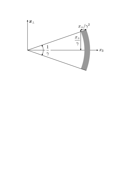
Figure 1: The region in space–time allowed by causality and special relativity for the matter distribution produced by the decaying photon in a highly boosted frame. More precisely, the gray band represents the boosted version of the half sphere $\{r\leq t;x_{3}>0\}$ (the region which, in the rest frame, includes the quanta whose velocities have a positive third component ($v_{3}>0$).

It is finally convenient, before concluding this section, to anticipate the typical resolution scales that we shall need in order to probe the structure of the decaying system. This can be fixed by comparison with the maximal (transverse and longitudinal) sizes occupied by the system, that we shall now estimate. For simplicity, we start in the rest frame of the time–like photon, where the matter produced by its decay is restricted to the sphere $r\leq t$, simply by causality. When boosting this spherical distribution with a large $\gamma$ factor, its transverse size remains unchanged, that is, $\Delta x_{\perp}\sim t_{RF}\sim t/\gamma$. (We used the fact that the time $t$ in the laboratory frame is larger by a factor $\gamma$ than the time $t_{RF}$ in the rest frame.) As for the longitudinal extent $\Delta x_{3}$, this is subjected to Lorentz contraction, yielding $\Delta x_{3}\sim t_{RF}/\gamma\sim t/\gamma^{2}$. The fastest partons propagate at the speed of light, so they will be located on the light–cone $x_{3}=t$ (or $x_{-}=0$). Most of the other partons, which are expected to be time–like and thus have velocities smaller than one, will be distributed within a region $\Delta x_{3}\sim t/\gamma^{2}$ behind the light–cone. Hence, the matter produced by the decay at light–cone time $\tau$ will be located within a small solid angle $\Delta\Omega\sim(\Delta x_{\perp}/\tau)^{2}\sim 1/\gamma^{2}$ around the $x_{3}$ axis and within a (relatively) thin longitudinal shell $\Delta x_{-}\sim\tau/\gamma^{2}$ around $x_{-}=0$. This region is represented as a grey band in Fig. 1. To be able to explore its internal structure, we need a probe with sufficiently large spatial momenta $\Delta_{+}\gtrsim\gamma^{2}/\tau$ and $\Delta_{\perp}\gtrsim\gamma/\tau$. But the opposite case, with $\Delta_{+}\ll\gamma^{2}/\tau$, is also interesting, since then the probe measures the matter distribution integrated over the longitudinal (or radial) axis. From the previous discussion, we expect a three–point function to be a good measurement (say, of the energy) when $\Delta_{+}\ll\gamma^{2}/\tau$ — in which case it correctly provides the energy density per unit transverse area (or per unit solid angle in the photon rest frame) —, but not also in the opposite case ($\Delta_{+}\gtrsim\gamma^{2}/\tau$), where the longitudinal resolution is relatively high. These expectations will be confirmed by the subsequent calculations, at both strong and weak coupling.

3 The three–point function at infinitely strong coupling

In this section we shall briefly review a recent calculation Hatta:2010dz of the three–point function introduced in Eq. (2.10) in the $\mathcal{N}=4$ SYM theory at (infinitely) strong coupling, which uses the method of the ‘backreaction’ within the dual supergravity theory. An alternative method, which relies on Witten diagrams for supergravity and is perhaps more straightforward to use for the calculation of the four–point functions, will be presented in Sect. 6.

3.1 Backreaction in supergravity

Within the AdS/CFT correspondence, a time–like photon decaying in the vacuum of the ${\mathcal{N}}=4$ SYM theory with infinitely strong ’t Hooft coupling ($\lambda\equiv g^{2}N_{c}\to\infty$) is dual to a supergravity (SUGRA) vector field $A^{\mu}(x,z)$ which propagates into the bulk of AdS₅ and whose boundary value $A^{\mu}(x,0)$ at the Minkowski boundary ($z=0$) is identified with the classical field $A^{\mu}_{q}(x)$ representing the perturbation on the gauge theory side: $A^{\mu}_{q}(x)=\varepsilon^{\mu}\,\phi_{q}(x)$ with the wave–packet $\phi_{q}(x)$ given in Eq. (2.7).

Within this franework, the first three–point function in (2.10) (the ‘energy density’ $\mathcal{E}_{q}(x)$) can be determined via a backreaction calculation. This refers to the linear response of the metric of AdS₅ to the small perturbation represented by the bulk excitation induced by the boundary WP (2.7). In turn, this bulk excitation can be obtained by propagating the boundary field with the help of the relevant bulk–to–boundary propagator (the Green’s function for the Maxwell equation in AdS₅) :

$$A^{\mu}_{q}(x,z)\,=\,\int\,{\rm d}^{4}y\,D^{\mu\nu}(x-y,z)\,\varepsilon_{\nu}\,\phi_{q}(y)\,=\,\int\,\frac{{\rm d}^{4}p}{(2\pi)^{4}}\,{\rm e}^{ip\cdot x}\,\varepsilon_{\nu}\,D^{\mu\nu}(p,z)\,\phi_{q}(p)\,,$$ (3.15)

where $D^{\mu\nu}(x-y,z)$ is the Maxwell propagator in AdS₅ and in the ‘radial’ gauge $A_{z}=0$. Here, $z$ denotes the radial (or ‘fifth’) dimension in AdS₅ and we are using the metric (with $L$ the curvature radius of AdS₅)

$${\rm d}s^{2}\,\equiv\,G_{MN}\,{\rm d}x^{M}{\rm d}x^{N}\,=\,\frac{L^{2}}{z^{2}}\,\big{[}-{\rm d}t^{2}+{\rm d}{\bm{r}}^{2}+{\rm d}z^{2}\big{]},$$ (3.16)

(with $M=\mu$ or $z$) in terms of which the Minkowski boundary lies at $z=0$, as anticipated.

The SUGRA field (3.15) will be explicitly constructed in Sect. 6.1 below, from which we anticipate here the salient features (see also Ref. Hatta:2010dz ). Namely, the bulk excitation is a Gaussian WP which propagates in AdS₅ at the 5–dimensional speed of light, with longitudinal velocity equal to $v$ and radial velocity $v_{z}=\sqrt{1-v^{2}}=1/\gamma$. More precisely, at time $t\gtrsim\sigma_{+}$, the center of the Gaussian is located at

$$z=\,\frac{t}{\gamma}\,,\qquad\bm{x}_{\perp}=0,\,\qquad x_{3}=vt\,,$$ (3.17)

with (roughly) time–independent widths fixed by the original Gaussian (2.7) (see Sect. 6.1 for details). The physical meaning of the bulk trajectory (3.17) can be understood with the help of the UV/IR correspondence Susskind:1998dq ; Peet:1998wn  : the penetration $z$ of the WP in the bulk is related to the virtuality $K=\sqrt{|k^{2}|}$ of the typical quanta composing the decaying WP in the boundary gauge theory: $z\sim 1/K$. (For the situation at hand, these quanta are typically time–like: $k^{2}<0$.) Hence, the fact that $z$ is localized near ${t}/{\gamma}$ means that the decaying system at time $t\gg\sigma_{+}$ involves quanta with a typical virtuality $K(t)\sim\gamma/t$ and hence a typical longitudinal momentum $k_{+}(t)=\gamma K(t)\sim\gamma^{2}/t$. By the uncertainty principle, such quanta occupy a region with transverse area $(\Delta x_{\perp})^{2}\sim(t/\gamma)^{2}$ and longitudinal extent $\Delta x_{3}\sim t/\gamma^{2}$ behind the light–cone ($x_{3}=t$). Note that this is the maximal region allowed by causality and special relativity (cf. the discussion towards the end of Sect. 2). This qualitative picture for the decaying system at strong coupling will be later substantiated, in Sect. 6, by a proper ‘measurement’ which involves the calculation of a four–point function. On the other hand, this picture is not manifest at the level of the three–point function $\mathcal{E}_{q}(x)$, to which we now turn.

The calculation of the backreaction amounts to solving the linearized Einstein equations for the (small) change $\delta G_{MN}$ in the metric of AdS₅ which is generated by the energy–momentum tensor $t^{MN}$ associated with the bulk excitation. Finally, the three–point function (2.10) is inferred from the near boundary behaviour of $\delta G_{MN}$. Mathematically, this is obtained by propagating the metric perturbation from the location $(\acute{x}^{\mu},z)$ of its source in the bulk to the measurement point $x^{\mu}$ on the boundary ($z=0$), with the help of the retarded bulk–to–boundary propagator. Strictly speaking, this calculation will yield a retarded three–point function — the retarded version of the Wightman function introduced in Eq. (2.10). But this retarded three–point function is precisely the physical response function whose space–time localization we would like to study.

For simplicity, we shall replace the bulk WP by a 4–dimensional $\delta$–function with support at the central coordinates shown in Eq. (3.17) : $t^{MN}(\acute{x},z)\propto\delta(\acute{x}_{3}-v\acute{t})\delta^{(2)}(\acute{\bm{x}}_{\perp})\delta(z-\acute{t}/\gamma)$. This means that we probe physics on space–time resolution scales which are soft compared to the respective widths of the Gaussian WP, which is indeed sufficient for our purposes here. This facilitates the calculation of the backreaction, which in general involves an integral over the support of the bulk excitation. The result of this calculation reads (see Ref. Hatta:2010dz and also the Appendix A to the present paper for details)

$$\mathcal{E}_{q}(t,\bm{x})\,=\, \frac{2q_{0}}{\pi}\,\frac{t+vx_{3}}{\gamma^{2}}\ \partial^{2}_{r^{2}}\int_{0}^{\infty}{\rm d}\acute{t}\,\acute{t}\ \delta\big{(}t^{2}-r^{2}-2(t-vx_{3})\acute{t}\big{)}$$

$$+\,\frac{2q_{0}}{\pi}\,\frac{v^{2}{x}_{\perp}^{2}}{\gamma^{2}}\ \partial^{3}_{r^{2}}\int_{0}^{\infty}{\rm d}\acute{t}\,\acute{t}^{\,2}\ \delta\big{(}t^{2}-r^{2}-2(t-vx_{3})\acute{t}\big{)},$$ (3.18)

where $r=|\bm{x}|$ and $q_{0}$ is the total energy carried by the original WP (2.7) (and therefore also the total energy of the evolving partonic system produced by its decay). Below we shall denote the two terms in Eq. (3.1) as $\mathcal{E}_{A}$ and $\mathcal{E}_{B}$, respectively, with $\mathcal{E}_{q}=\mathcal{E}_{A}+\mathcal{E}_{B}$. In the original calculation in Ref. Hatta:2010dz , the second term $\mathcal{E}_{B}$ has actually been missed, so for completeness we shall explicitly derive this term in Appendix A.

Eq. (3.1) can be understood as follows: at time $\acute{t}$, the bulk excitation localized at $z=\acute{t}/\gamma$, $\acute{x}_{3}=v\acute{t}$, and $\acute{x}_{\perp}=0$ emits a gravitational wave $\delta G_{MN}$ which propagates through AdS₅ at the respective speed of light up to the measurement point $x^{\mu}=(t,\bm{x})$ on the boundary. The $\delta$–function in the integrand represents the support of the retarded bulk–to–boundary propagator for the Einstein equations in AdS₅. Its argument follows from causality together with the condition of propagation at the 5D speed of light, for both the bulk excitation and the gravitational wave:

$$(t-\acute{t}\,)^{2}={z}^{\,2}+(x_{3}-\acute{x}_{3})^{2}+x_{\perp}^{2}={{\acute{t}}^{\,2}+r^{2}-2x_{3}v\acute{t}}\ \Longrightarrow\ t^{2}-r^{2}=2(t-vx_{3})\acute{t}\,.$$ (3.19)

A physical interpretation for this condition back in the original gauge theory will be proposed in Sect. 3.2.

A priori, Eq. (3.1) involves an integral over all the positive values of $\acute{t}$, meaning over all the values $z=\acute{t}/\gamma$ of the radial coordinate of the bulk excitation. However, the presence of the external derivatives, $\partial^{2}_{r^{2}}$ in the first term and respectively $\partial^{3}_{r^{2}}$ in the second one, introduces an important simplification: it implies that the net result for $\mathcal{E}_{q}$ comes exclusively from $\acute{t}=0$, that is, from the early time when the bulk excitation had been just emitted and was still localized near the boundary ($z\simeq 0$). Indeed, after using the $\delta$–function to integrate over $\acute{t}$, one finds

$$\mathcal{E}_{q}(x)\,=\, \frac{q_{0}}{2\pi\gamma^{2}}\,\frac{t+vx_{3}}{(t-vx_{3})^{2}}\ \partial^{2}_{r^{2}}[(t^{2}-r^{2})\Theta(t^{2}-r^{2})]$$

$$+\,\frac{q_{0}}{4\pi\gamma^{2}}\,\frac{v^{2}{x}_{\perp}^{2}}{(t-vx_{3})^{3}}\ \partial^{3}_{r^{2}}[(t^{2}-r^{2})^{2}\Theta(t^{2}-r^{2})],$$ (3.20)

where the $\Theta$–function enforcing $r\leq t$ (generated via the condition that $\acute{t}\geq 0$) is the expression of causality. In the first term, this $\Theta$–function is multiplied by the factor $(t^{2}-r^{2})$ which is linear in $r^{2}$; so the only way to obtain a non–zero result after acting with $\partial^{2}_{r^{2}}$ is that one of the two derivatives act on the $\Theta$–function and thus generate a $\delta$–function at $t=r$. A similar discussion applies to the second term, which involves an additional factor of $(t^{2}-r^{2})$ inside the square brackets and also an additional external derivative. Combining the two terms, one finds

$$\mathcal{E}_{q}(x)\,=\,\frac{q_{0}}{2\pi\gamma^{4}}\,\frac{t^{2}}{(t-vx_{3})^{3}}\,\delta(t^{2}-r^{2})\,.$$ (3.21)

This describes a spherical shell of zero width which propagates at the 4–dimensional speed of light. Returning to the constraint (3.19) on the emission time $\acute{t}$, one sees that a signal which at time $t$ is located at $r=t$ has been necessarily generated at $\acute{t}=0$ and hence $z=0$, as anticipated.

Now, as it should be clear from the previous discussion, these extremely sharp localization properties — the fact that the signal is strictly light–like ($r=t$) and the (related) fact that the whole contribution to the backreaction comes from $z=0$ — are to be understood up to a smearing on the scale set by the width $\sigma$ of the original WP : in reality, the spherical shell has a non–zero radial width $t-r\sim\sigma$ and the values of $z$ contributing to this result are not exactly zero, but of order $\sigma$. Yet, these results — in particular, the fact that the signal appears to propagate without broadening (i.e. by preserving a constant radial width up to arbitrarily large times) — would be extremely curious if they were to represent the distribution of matter produced by a decaying system at strong coupling, as we now explain.

A thin shell of energy propagating at the speed of light is the result that would be naturally expected in a non–interacting quantum field theory, or, more generally, to zeroth order in perturbation theory for a field theory at weak coupling. In that limit, the time–like photon would decay into a pair of (massless) on–shell partons which would then propagate at the speed of light. In a given event and in the rest frame of the virtual photon, such a decay yields two particles propagating back to back. After averaging over many events, the signal looks like a thin spherical shell expanding at the speed of light. In fact, it is straightforward to check (and we shall explicitly do that in the next sections) that the result (3.21) of the AdS/CFT calculation at infinitely strong coupling is exactly the same as the corresponding prediction of the $\mathcal{N}=4$ SYM theory at zero coupling. By itself, this ‘coincidence’ should not be a surprise: as explained in the Introduction, the three–point function under consideration cannot receive quantum corrections, as it is protected by conformal symmetry and energy conservation. So, the corresponding result, as shown in Eq. (3.21), is a priori known to be independent of the coupling. But whereas this situation looks natural in view of the underlying conformal symmetry, it might still look puzzling from a physical perspective: at non–zero (gauge) coupling, the decay of the time–like photon should also involve virtual quanta which propagate slower than light. Then, the emerging matter distribution should also have support at points inside the sphere $r\leq t$, and not only on its (light–like) surface.

The solution to this puzzle is that, as already argued in Sect. 2 and will be demonstrated via explicit calculations in what follows, this three–point function is not a good measurement of the energy density produced at late times by the decaying photon. It is clearly a good measurement of its total energy, and also of its angular distribution in the photon’s rest frame ($v=0$), where Eq. (3.21) yields the expected result for ${{\rm d}E}/{{\rm d}\Omega}$ (recall that $q_{0}\to Q$ in the rest frame) :

$$\mathcal{E}_{q}(t,r)\,=\,\frac{Q}{4\pi r^{2}}\,\delta(t-r)\qquad\Longrightarrow\qquad\frac{{\rm d}E}{{\rm d}\Omega}\,\equiv\int{\rm d}r\,r^{2}\mathcal{E}_{q}\,=\,\frac{Q}{4\pi}\,.$$ (3.22)

But the radial distribution of the energy density is not correctly represented by Eq. (3.21), in any frame. The correct respective distribution will be later computed, at both weak and strong coupling, from four–point functions like those introduced in Eq. (2.11). The results to be thus obtained will be very different in the two cases and in particular they will exhibit strong radial broadening at strong coupling, in agreement with our general expectations. This being said, it would be interesting to understand ‘how the conformal symmetry works in practice’, meaning how is that possible that such a sharply localized result, Eq. (3.21), can emerge from a calculation at strong coupling. A possible interpretation for that will be provided in the next subsection.

For what follows, it will be useful to have a version of the three-point function (3.21) adapted to a highly boosted frame ($\gamma\gg 1$). In that case, it is preferable to work with the probe operator ${\hat{T}}_{++}(x)$ and the associated three–point function $\mathcal{P}_{q}(x)$, as introduced in Eq. (2.10). At high energy, the latter can be estimated as $\mathcal{P}_{q}(x)\simeq 2\mathcal{E}_{q}(x)$ with $\mathcal{E}_{q}(x)$ conveniently rewritten in light–cone coordinates. Using $1-v\simeq 1/2\gamma^{2}$, $1+v\simeq 2$, and hence

$$t-vx_{3}\,=\,\frac{x_{+}(1-v)+x_{-}(1+v)}{\sqrt{2}}\,\simeq\,\frac{x_{+}}{2\sqrt{2}\gamma^{2}}\,+\sqrt{2}x_{-}\,,$$ (3.23)

one finds (with $q_{+}\simeq\sqrt{2}q_{0}$)

$$\mathcal{P}_{q}(x)\,\simeq\,\frac{q_{+}}{8\pi\gamma^{4}}\,\frac{x_{+}^{2}}{\Big{(}x_{-}+\frac{x_{+}}{4\gamma^{2}}\Big{)}^{3}}\,\delta\left(2x_{+}x_{-}-{x}_{\perp}^{2}\right).$$ (3.24)

The denominator in this equation is the reflection of Lorentz contraction, as discussed at the end of Sect. 2 : it restricts the longitudinal coordinate $x^{-}$ to (positive) values satisfying $x_{-}\lesssim{x_{+}}/4\gamma^{2}$. But the presence of the $\delta$–function in Eq. (3.24) entails a much stronger constraint: it implies that the signal is localized within an arc of a spherical shell of zero width, or more precisely of width $\sigma_{-}\sim\sigma/\gamma$ (the Lorentz–contracted version of the respective width in the rest frame). This distribution is illustrated in Fig. 2 which should be compared with Fig. 1. One sees that, in the boosted frame, the lack of radial broadening mostly manifests itself as a lack of longitudinal broadening: the signal (3.24) deviates from the light–cone ($x_{-}=0$) by a distance $x_{-}=x_{\perp}^{2}/2x_{+}$ (modulo the width $\sigma_{-}$ of the shell) which for sufficiently small $x_{\perp}\ll x_{+}/\gamma$ is much smaller than the maximal value $\sim{x_{+}}/\gamma^{2}$ permitted by Lorentz contraction. Conversely, this argument implies that $x_{\perp}$ is restricted to values $x_{\perp}\lesssim x_{+}/\gamma$, which in turn implies that the solid angle subtended by the shell is $\delta\Omega\sim 1/\gamma^{2}$. Note finally that Eq. (3.24) yields the correct result for the total longitudinal momentum (cf. Eq. (2.12)), as expected: $P_{q}\equiv\int{\rm d}x^{-}{\rm d}^{2}x_{\perp}\,\mathcal{P}_{q}=q_{+}$.

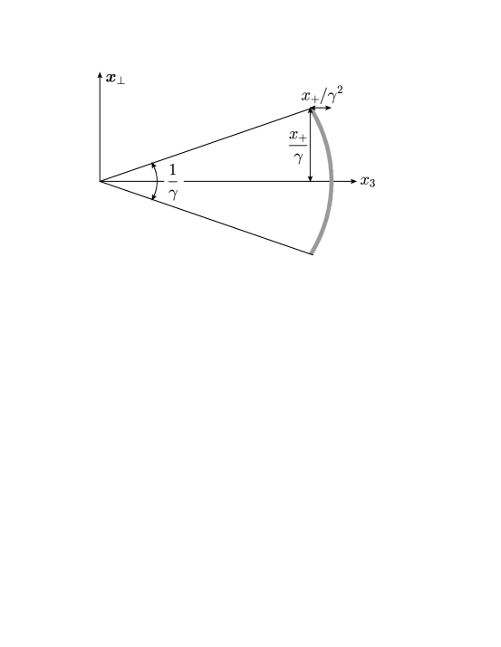
Figure 2: Signal generated from the decaying photon in a highly boosted frame. The width of the grey band is $\sigma_{-}\sim\sigma/\gamma$ (the Lorentz contracted version of the radial width in the rest frame).

3.2 A physical interpretation for the ‘backreaction’

As already noticed, the SUGRA results for the three–point function, (3.21) or (3.24), are characterized by two remarkable and perhaps surprising facts: (i) the signal propagates at the speed of light without (radial or longitudinal) broadening, and (ii) the whole contribution to the backreaction comes from small values of $z\lesssim\sigma$. Within the AdS/CFT calculation, these two features are related to each other, as we have seen. Namely, the ‘backreaction’ has support only at points satisfying Eq. (3.19), which for small $z=\acute{t}/\gamma\lesssim\sigma$ implies that $t-r$ (or $t-x_{3}$ in a boosted frame) is small as well: $t-r\lesssim\sigma$ in the center–of–mass frame and respectively $x_{-}\lesssim\sigma/\gamma$ in the frame where $\gamma\gg 1$. That is, the smallness of $z$ (or of $\acute{t}$) implies the propagation of the signal at the speed of light. In what follows, we would like to propose a physical interpretation for these facts in the CFT.

Namely, we shall argue that the interactions responsible for the three–point function are highly delocalized in time. The high–momentum transfer between the target and the probe is carried by a signal which is emitted by the decaying system at an early time, well before the measurement time $t$ at which the signal is absorbed by the probe. This physical emission time (denoted as $t_{\rm int}$ in the Introduction) can be identified with the time $\acute{t}$ at which the gravitational wave is emitted by the bulk excitation in the calculation of the backreaction. With this interpretation, Eq. (3.19) represents the matching condition between the resolution of the probe and the kinematics of the target ‘partons’ which emit the signal. Furthermore, the gravitational wave in the ‘backreaction’ is the AdS dual of the physical signal — a nearly light–like mode with the quantum numbers of the probe operator, which propagates at the speed of light from $\acute{t}$ up to $t$.

In order to establish this interpretation, we shall have a new look at Eq. (3.19) which we recall is the condition that the gravitational wave propagate at the speed of light in AdS₅. For a given observation point $x^{\mu}$ on the boundary, this condition determines the time $\acute{t}$ at which the gravitational wave is emitted, hence the radial penetration $z=\acute{t}/\gamma$ of the bulk excitation at that time and, ultimately, the virtuality $K=\sqrt{|k^{2}|}$ of the typical quanta composing the decaying system at time $\acute{t}$ : the UV/IR correspondence implies $K\simeq 1/z=\gamma/\acute{t}$. For what follows it is convenient to fix the transverse coordinate of the observation point — namely, we choose $x_{\perp}\simeq 0$ (with uncertainty $\sigma$) — and explore the longitudinal region behind the light–cone ($x_{-}=0$) on a resolution scale $\delta x_{-}$ which is allowed to vary. As usual, this resolution is controlled by the longitudinal momentum of the probe, $\delta x_{-}\simeq 1/\Delta_{+}$, and is limited by the longitudinal width $\sigma_{-}\sim\sigma/\gamma$ of the original wave–packet. The best possible resolution $\delta x_{-}\simeq\sigma_{-}$ (corresponding to a maximal momentum transfer $\Delta_{+}\sim\gamma/\sigma$) has been implicitly used in the calculation of the three–point function ‘at a given space–time point’, cf. Eq. (3.21) and (3.24). But for the present purposes we shall also allow for less precise measurements, with $\Delta_{+}\ll 1/\sigma_{-}$.

Starting with Eq. (3.19), inserting $x_{\perp}=0$ and $t-x_{3}=\sqrt{2}/\Delta_{+}$, and switching to light–cone coordinates, one easily finds (we use the notation $\tau\simeq\sqrt{2}t$ for the light–cone time of measurement and similarly $\acute{\tau}\simeq\sqrt{2}\acute{t}$ for the emission time)

$$\acute{\tau}\,\simeq\,\frac{\tau}{1+\frac{\tau\Delta_{+}}{4\gamma^{2}}}\,.$$ (3.25)

There are two interesting limiting cases:

(i) High longitudinal resolution:  $\Delta_{+}\gg\gamma^{2}/\tau$. In this case, the probe can discriminate longitudinal distances $\delta x_{-}\simeq 1/\Delta_{+}$ which are much smaller than the upper limit $\Delta x_{-}\sim\tau/\gamma^{2}$ enforced by causality and Lorentz contraction. Then Eq. (3.25) implies

$$\acute{\tau}\,\simeq\,\frac{4\gamma^{2}}{\Delta_{+}}\,\ll\,\tau.$$ (3.26)

It is also interesting to estimate (using the UV/IR correspondence) the typical virtuality and longitudinal momentum of a quantum from the target at time $\acute{\tau}$ :

$$K\,\simeq\,\frac{\sqrt{2}\gamma}{\acute{\tau}}\,\simeq\,\frac{\Delta_{+}}{2\sqrt{2}\gamma}\,,\qquad k_{+}\,\simeq\,\sqrt{2}\gamma\,K\simeq\,\frac{\Delta_{+}}{2}\,.$$ (3.27)

The last condition ($k_{+}\sim\Delta_{+}$) is very interesting: this is the expected matching condition between the quanta from the target which emit the relatively hard signal and the resolution of the probe. Remarkably, this condition holds here at the ‘emission time’ $\acute{\tau}$ and not at the measurement time $\tau$. This is in agreement with our expectation that such hard quanta can only exist at very early times in the history of the decay. In fact, the above results can be combined to yield $\acute{\tau}\simeq k_{+}/K^{2}$, which is the time interval required via the uncertainty principle for the emission of a quantum with longitudinal momentum $k_{+}$ and virtuality $K^{2}$. The above discussion makes it natural to identify the ‘emission time’ $\acute{t}$ (or $\acute{\tau}$) in the SUGRA calculation with the time at which the signal measured by the probe operator at time $t$ (or $\tau$) has been actually emitted by the decaying system in the underlying quantum field theory.

Returning to Eq. (3.25), let us also consider the other interesting limiting case, namely :

(ii) Low longitudinal resolution:  $\Delta_{+}\ll\gamma^{2}/\tau$. In this case, the probe cannot discriminate any longitudinal substructure, but, interestingly, it can explore the state of the system at relatively late times, close to the time $\tau$ of measurement. Indeed, Eq. (3.25) implies

$$\acute{\tau}\,\simeq\,\tau\,,\qquad K\,\sim\,\frac{\gamma}{\tau}\,,\qquad k_{+}\,\sim\,\frac{\gamma^{2}}{\tau}\,.$$ (3.28)

This can be understood as follows: the probe is now much softer ($\Delta_{+}\ll k_{+}$) than the typical quanta in the decaying system at time $\tau$, so it can interact with the latter without significantly disturbing them.

So far, we have considered a probe with a fixed longitudinal resolution $\delta x_{-}\simeq 1/\Delta_{+}$, that is, we have focused on a single Fourier mode, with longitudinal momentum $\Delta_{+}$, of the probe operator. But a similar discussion applies to a three–point function in coordinate space, like $\mathcal{E}_{q}(x)$. The associated Fourier decomposition involves an integral over all values of $\Delta_{+}$, but in practice this integral is dominated by its upper limit $\Delta_{+}\sim\gamma/\sigma$, which is the maximal value allowed by energy–momentum conservation. Then, Eq. (3.26) implies $\acute{\tau}\sim\gamma\sigma$ and therefore $z\sim\sigma$. This explains why the whole contribution to the backreaction ‘at a given space–time point’ comes from very small $z\lesssim\sigma$. The fact that the signal propagates at the speed of light and without broadening can be qualitatively understood as a consequence of kinematics. Given that this signal is carried along by essentially a single mode of the probe — the one with the maximal value of $\Delta_{+}$ —, it naturally preserves a constant width $\delta x_{-}\sim\sigma/\gamma$. And a signal which propagates with $t-x_{3}=$ const. over a large period of time is necessarily luminal.

To summarize, a three–point function with high longitudinal resolution explores the state of the target at very early time, much smaller than the time of measurement $t$. Conversely, the only way how a three–point function can measure the state of the target at $t$ is by giving up any precision in the longitudinal (or radial) direction. These conclusions will be corroborated by the Fourier decomposition of the three–point function to be presented in the next subsection.

3.3 Momentum–space analysis of the backreaction

In this subsection, we shall compute the Fourier transform of the result in Eq. (3.24) for the three–point function in a highly boosted frame. We shall use a mixed Fourier representation which involves the component ${\hat{T}}_{++}(\tau,\Delta_{+},{\bm{\Delta}}_{\perp})$ of the probe operator. As explained towards the end of Sect. 2, this mixed representation contains the essential information that we need about the probe, namely the time of measurement $\tau$, assumed to be large ($\tau\gg\sigma_{+}$), and the associated, longitudinal and transverse, resolutions: $\delta x_{-}\sim 1/{\Delta_{+}}$ and $\delta x_{\perp}\sim{1}/{\Delta_{\perp}}$.

This change of representation is useful for several purposes. First, it will facilitate the comparison with the zeroth order calculation at weak coupling, to be presented in the next section. Second, it will substantiate the argument developed in the previous subsection, concerning the correlation between the resolution of the probe and the time of interaction (cf. Eq. (3.25)) . Third, it will allow us to explicitly check that the narrow signal seen in coordinate space corresponds to a light–like mode of the probe operator. For the latter purposes, it is preferable to perform the Fourier transform before computing the integral over $\acute{t}$ in Eq. (3.1).

Consider for illustration the first term, ${\mathcal{E}}_{A}$, in Eq. (3.1). By using simplifications appropriate at high energy, cf. Eq. (3.23), and changing the integration variable from $\acute{t}$ to $z=\acute{t}/\gamma$, we obtain

$$\tilde{\mathcal{E}}_{A}(\tau,\Delta_{+},{\bm{\Delta}}_{\perp}) \,\equiv\,\int{\rm d}x_{-}{\rm d}^{2}\bm{x}_{\perp}{\rm e}^{i\Delta_{+}x_{-}-i{\bm{\Delta}}_{\perp}\cdot\bm{x}_{\perp}}\,\mathcal{P}_{A}(\tau,x_{-},\bm{x}_{\perp})$$ (3.29)

$$\,=\,\frac{2q_{+}\tau}{\pi} \int{\rm d}x_{-}{\rm d}^{2}\bm{x}_{\perp}{\rm d}z\,z\,\delta^{\prime\prime}\bigg{(}2x_{-}\big{(}\tau-\sqrt{2}\gamma z\big{)}-x_{\perp}^{2}-\frac{z\tau}{\sqrt{2}\gamma}\bigg{)}\,{\rm e}^{i\Delta_{+}x_{-}-i{\bm{\Delta}}_{\perp}\cdot\bm{x}_{\perp}}\,\,.$$

The double prime on the $\delta$–function within the integrand denotes two derivatives w.r.t. its argument. It is convenient to rewrite one of them as a derivative w.r.t. $z$ and perform an integration by parts to deduce

$$\tilde{\mathcal{E}}_{A}\,=\,{4q_{+}\tau}\int\frac{{\rm d}x_{-}{\rm d}x_{\perp}{\rm d}z}{2\sqrt{2}\gamma x_{-}+\frac{\tau}{\sqrt{2}\gamma}}\,\delta^{\prime}\bigg{(}2x_{-}\big{(}\tau-\sqrt{2}\gamma z\big{)}-x_{\perp}^{2}-\frac{z\tau}{\sqrt{2}\gamma}\bigg{)}x_{\perp}{\rm J}_{0}(\Delta_{\perp}x_{\perp})\,{\rm e}^{i\Delta_{+}x_{-}}\,\,.$$ (3.30)

The Bessel function ${\rm J}_{0}(\Delta_{\perp}x_{\perp})$ has been generated by the angular integration over the azimuthal angle of $\bm{x}_{\perp}$. We shall now express the remaining derivative of the $\delta$–function as a derivative w.r.t. $x_{\perp}$ and again perform an integration by parts, to obtain (recall that ${\rm J}_{1}(x)=-{\rm d}{\rm J}_{0}/{\rm d}x$)

$$\tilde{\mathcal{E}}_{A}\,=\,{2q_{+}\tau}\int\frac{{\rm d}x_{-}{\rm e}^{i\Delta_{+}x_{-}}}{2\sqrt{2}\gamma x_{-}+\frac{\tau}{\sqrt{2}\gamma}}\left\{\frac{1}{2\sqrt{2}\gamma x_{-}+\frac{\tau}{\sqrt{2}\gamma}}-\,\frac{\Delta_{\perp}}{2}\int_{0}^{z_{\rm max}}{\rm d}z\,\frac{{\rm J}_{1}\big{(}\Delta_{\perp}X_{\perp}(z)\big{)}}{X_{\perp}(z)}\right\}\,.$$ (3.31)

In writing the above, we have also used the $\delta$–function to perform the integral over $z$ in the first term within the accolades (the boundary term) and respectively the integral over $x_{\perp}$ in the second term, and we have denoted

$$X_{\perp}(z)\,\equiv\,\sqrt{2x_{-}\tau-z\Big{(}2\sqrt{2}\gamma x_{-}+\frac{\tau}{\sqrt{2}\gamma}\Big{)}}\,.$$ (3.32)

The upper limit $z_{\rm max}$ in the integral over $z$ is determined by the condition $X_{\perp}(z_{\rm max})=0$, which yields

$$z_{\rm max}\,=\,\frac{1}{\sqrt{2}\gamma}\,\frac{\tau}{1+\frac{\tau}{4\gamma^{2}x_{-}}}\,.$$ (3.33)

Recalling that $z=\acute{t}/\gamma\simeq\acute{\tau}/\sqrt{2}\gamma$ and using $x_{-}\lesssim 1/\Delta_{+}$, this upper limit is clearly consistent with our previous estimate for the (maximal) emission time $\acute{\tau}$ in Eq. (3.25).

We now change variables in the integral over $z$ according to $z\to\xi\equiv\Delta_{\perp}X_{\perp}(z)$, which gives

$$\tilde{\mathcal{E}}_{A}\,=\, {2q_{+}\tau}\int\frac{{\rm d}x_{-}{\rm e}^{i\Delta_{+}x_{-}}}{\Big{[}2\sqrt{2}\gamma x_{-}+\frac{\tau}{\sqrt{2}\gamma}\Big{]}^{2}}\left\{1-\int_{0}^{\Delta_{\perp}\sqrt{2x_{-}\tau}}{\rm d}\xi\,{\rm J}_{1}(\xi)\right\}$$

$$\,=\, {4q_{+}}\,\frac{\gamma^{2}}{\tau}\,\int\frac{{\rm d}x_{-}{\rm e}^{i\Delta_{+}x_{-}}}{\Big{[}1+\frac{4\gamma^{2}x_{-}}{\tau}\Big{]}^{2}}\,{\rm J}_{0}\big{(}\Delta_{\perp}\sqrt{2x_{-}\tau}\,\big{)}\,.$$ (3.34)

The Fourier transform of the second term ${\mathcal{E}}_{B}$ in Eq. (3.1) can be similarly computed (in particular, this introduces the same upper limit $z_{\rm max}$ on $z$ as shown in Eq. (3.33)) and the final result reads

$$\tilde{\mathcal{P}}_{q}\,\simeq\,2\big{(}\tilde{\mathcal{E}}_{A}+\tilde{\mathcal{E}}_{B}\big{)}\,=\,{8q_{+}}\,\frac{\gamma^{2}}{\tau}\,\int\frac{{\rm d}x_{-}{\rm e}^{i\Delta_{+}x_{-}}}{\Big{[}1+\frac{4\gamma^{2}x_{-}}{\tau}\Big{]}^{3}}\,{\rm J}_{0}\big{(}\Delta_{\perp}\sqrt{2x_{-}\tau}\,\big{)}\,,$$ (3.35)

where we have used the relation ${\mathcal{P}}_{q}\simeq\ 2{\mathcal{E}}_{q}$ valid at high energy.

In order to evaluate the remaining integral over $x_{-}$, we shall perform approximations appropriate to the two interesting limiting regimes: $\Delta_{+}\gg\gamma^{2}/\tau$ and respectively $\Delta_{+}\ll\gamma^{2}/\tau$.

(i) High longitudinal resolution:  $\Delta_{+}\gg\gamma^{2}/\tau$. In this case, the typical values of $x_{-}$ contributing to the integral in Eq. (3.35) obey $x_{-}\lesssim 1/{\Delta_{+}}\ll\tau/\gamma^{2}$, so one can neglect the second term in the denominator of the integrand. This yields

$$\tilde{\mathcal{P}}_{q}\,\simeq\ {8q_{+}}\,\frac{\gamma^{2}}{\tau}\,\int_{0}^{\infty}{{\rm d}x_{-}{\rm e}^{i\Delta_{+}x_{-}}}\ {\rm J}_{0}\big{(}\Delta_{\perp}\sqrt{2x_{-}\tau}\,\big{)}\,=\,i\,{8q_{+}}\,\frac{\gamma^{2}}{\tau\Delta_{+}}\,{\rm e}^{-i\frac{\Delta_{\perp}^{2}}{2\Delta_{+}}\tau}\,.$$ (3.36)

The complex exponential can be rewritten as ${\rm e}^{-i\Delta_{-}\tau}$ with $\Delta_{-}={\Delta_{\perp}^{2}}/{2\Delta_{+}}$. This relation ${2\Delta_{+}\Delta_{-}}={\Delta_{\perp}^{2}}$ is recognized as the mass–shell condition for a light–like mode. (In fact, if one performs the remaining Fourier transform $\tau\to\Delta_{-}$ in Eq. (3.36), one finds a result proportional to $\delta(2\Delta_{+}\Delta_{-}-\Delta_{\perp}^{2})$.) This light–like mode with high longitudinal resolution is emitted at the early time $\acute{\tau}\sim\gamma^{2}/\Delta_{+}\ll\tau$ and then propagates at the speed of light up to the measurement time $\tau$. The Fourier transform of Eq. (3.36) back to coordinate space is dominated by the highest possible values for $\Delta_{+}$, namely $\Delta_{+}^{\rm max}\simeq\gamma/\sigma$, which explains why the support of the signal in coordinate space lies on the light–cone ($x_{-}\simeq x_{\perp}^{2}/2x_{+}$), with an uncertainty $\delta x_{-}\sim\sigma_{-}$ introduced by the width of the original wave–packet.

(ii) Low longitudinal resolution:  $\Delta_{+}\ll\gamma^{2}/\tau$. In this case, the typical values of $x_{-}$ contributing to the integral in Eq. (3.35) are determined either by the Bessel function, which implies $x_{-}\lesssim 1/(\tau\Delta_{\perp}^{2})$, or by the denominator of the integrand, which requires $x_{-}\lesssim\tau/\gamma^{2}$. The last constraint implies that $\Delta_{+}x_{-}\ll 1$ irrespective of the value of $\Delta_{\perp}$, so we can replace ${\rm e}^{i\Delta_{+}x_{-}}\simeq 1$. The ensuing integral over $x_{-}$ can be exactly computed by changing variables according to $x_{-}\equiv(\tau/4\gamma^{2})u^{2}$ :

$$\tilde{\mathcal{P}}_{q}\,\simeq\, 4q_{+}\int_{0}^{\infty}\frac{{\rm d}u\,u}{(1+u^{2})^{3}}\,{\rm J}_{0}\bigg{(}\frac{\Delta_{\perp}\tau}{\sqrt{2}\gamma}\,u\bigg{)}\,=\,\frac{q_{+}}{2}\bigg{(}\frac{\Delta_{\perp}\tau}{\sqrt{2}\gamma}\bigg{)}^{2}{\rm K}_{2}\bigg{(}\frac{\Delta_{\perp}\tau}{\sqrt{2}\gamma}\bigg{)}\,\,,$$ (3.37)

with ${\rm K}_{2}$ the modified Bessel function of rank 2. Using $(x^{2}/2)\mathrm{K}_{2}(x)\simeq 1$ for $x\ll 1$, we deduce that $\tilde{\mathcal{P}}_{q}\simeq q_{+}$ when $\Delta_{\perp}\ll\gamma/\tau$. This is as expected: by causality, the decaying sytem has a transverse size $\Delta x_{\perp}\sim\tau/\gamma$ and a longitudinal size $\Delta x_{-}\lesssim\tau/\gamma^{2}$ , so when this is probed with much poorer, transverse and longitudinal, resolutions, one sees the total energy $q_{+}$. In the opposite limit $\Delta_{\perp}\gg\gamma/\tau$, the signal is exponentially suppressed (we recall that $\mathrm{K}_{2}(x)\simeq\sqrt{{\pi}/{2x}}\,{\rm e}^{-x}$ for $x\gg 1$), meaning that the three–point function does not exhibit any substructure with transverse size much smaller than the overall size $\Delta x_{\perp}\sim\tau/\gamma$. This is again as expected: when integrated over $x_{-}$, the three–point function looks uniform in the transverse plane (at least, at points $x_{\perp}\ll\tau/\gamma$) simply by symmetry, that is, as a consequence of the spherical symmetry of the signal in the target rest frame. This can be also verified directly in coordinate space: by integrating Eq. (3.24) over $x_{-}$ or, equivalently, by performing the transverse Fourier transform in Eq. (3.37), one finds

$$\mathcal{P}_{q}(\tau,x_{\perp})\,\equiv\int{\rm d}x_{-}\,\mathcal{P}_{q}(x)\,\simeq\,\frac{q_{+}}{2\pi\gamma^{4}}\,\frac{\tau^{4}}{\Big{(}x_{\perp}^{2}+\frac{\tau^{2}}{2\gamma^{2}}\Big{)}^{3}}\,.$$ (3.38)

Notice that the low resolution modes are typically space–like : one has indeed $\Delta_{\perp}\sim\gamma/\tau$ and $\Delta_{-}\sim 1/\tau$, hence $\Delta_{\perp}^{2}\gg 2\Delta_{+}\Delta_{-}$. Consider also the typical values of $z$ and $\acute{t}$ contributing to the signal in Eq. (3.37). By using Eq. (3.33) together with $x_{-}\sim\tau/\gamma^{2}$, one finds $z_{\rm max}\sim\tau/\gamma$, which implies that $\acute{t}=\gamma z$ is commensurable with $\tau$. Thus, as already argued in the previous subsection, a three–point function with small $\Delta_{+}$ interacts with the target at times which are close to the time of measurement. Yet, because of the low longitudinal resolution, this does not bring us any additional information about the state of the system at $t$. The only physically relevant information that we can extract from the three–point function is the energy density per unit transverse area, Eq. (3.38), and this is independent of the actual interaction time (as it involves an integration over all longitudinal coordinates).

4 The three–point function at zero coupling

In this section, we shall calculate the three–point function (2.10) in $\mathcal{N}=4$ SYM in the other extreme limit: that of a zero coupling. Our main purpose is to verify that the final result is exactly the same as at infinitely strong coupling, as expected from the following facts: (i) in a conformal theory like $\mathcal{N}=4$ SYM the general structure of a three–point function is fixed by conformal symmetry together with the (quantum) dimensions of the involved operators, and (ii) the ${\mathcal{R}}$–current and the energy–momentum tensor are conserved quantities which are not renormalized, that is, they have no anomalous dimensions. Accordingly, the matrix element given in Eq. (2.10) must be independent of the coupling, and this is what shall explicitly check in what follows.

The result of the zeroth order calculation can be easily anticipated. In this limit the time–like ${\mathcal{R}}$–current decays into a fermion–antifermion (or scalar–antiscalar) pair, which then propagates without further evolution. In the center of mass frame of the decay, two back–to–back particles moving at the speed of light emerge. The three–point function is not sensitive to correlations between the directions of the two decay products, so the answer, in coordinate space, should look the same as that of a thin spherical shell of energy whose radius increases with the velocity of light. In the boosted frame in which we shall actually do the calculation, the energy distribution should be contracted to the part of the spherical shell having solid angle of size $1/\gamma^{2}$ around the longitudinal axis (the $x_{3}$ axis along which the decaying current is moving). As we shall see, this simple picture is indeed faithfully reflected by the zeroth order result for the three–point function. But as we shall later argue, this ability of the three–point function to properly reflect the partonic structure of the decaying system is in fact limited to zeroth order: it does not hold anymore after including perturbative corrections at weak but non–zero coupling.

As before, we shall assume that the momentum components, $\Delta^{\mu}$, of the energy–momentum tensor ${\hat{T}}_{++}$, are much less than the momentum of the ${\mathcal{R}}$–current initiating the decay. Thus, although we are evaluating a transition matrix element, the insertion of ${\hat{T}}_{++}$ affects the decay products in such a tiny way that the matrix element corresponds to a faithful determination of the average energy flow in the decay. This is of course limited to the present, zeroth order, calculation, in which the two partons produced by the original decay do not have the possibility to evolve anymore.

The fact that the three–point function in a conformal field theory is independent of the coupling means that, in perturbation theory at least, this quantity cannot correctly describe the flow of energy at non–zero coupling, where branchings of the decay products occur. The quantum evolution of the partons is on the other hand manifest in the perturbative evaluation of the four–point function, to be presented in the next two sections. As we shall see there, this evolution leads, at both weak and strong coupling, to the longitudinal broadening of the energy flow in the decay.

4.1 The decay rate

Our focus in the subsequent calculations at weak coupling will be on the description of the average properties of the matter distribution produced by the decay of a time–like ${\mathcal{R}}$–current in the $\mathcal{N}=4$ SYM theory. To that end it will be useful to have an evaluation of the decay rate $\Gamma$ of the ${\mathcal{R}}$–current, an operation which will also allow to introduce our notations. Indeed, in this perturbative context, the three–point and four–point functions to be later computed need to be divided by $\Gamma$ to ensure that they describe properties of a single decay.

To lowest in perturbation theory, meaning to zeroth order in the gauge coupling $g$ of $\mathcal{N}=4$ SYM and to order $e^{2}$ in the ‘electromagnetic coupling’ associated with the ${\mathcal{R}}$–charge, the ${\mathcal{R}}$–current can decay into either a fermion–antifermion pair, or into a pair of scalars. To keep the presentation as simple as possible, we shall only explicitly evaluate the decay into fermions and then simply indicate the changes which occur when adding the scalars. As before, we shall work with an ${\mathcal{R}}$–current boosted along the positive $x_{3}$ axis, with $q_{+}={Q^{2}}/{2q_{-}}\simeq\sqrt{2}\gamma Q$ and we shall evaluate the rate of decay $\Gamma_{+}$ per unit of light–cone time $x_{+}$. To the order of interest and for the decay into a pair of fermions, this reads

$$\Gamma_{+}\,=\int\frac{{\rm d}^{3}p}{(2\pi)^{3}2p_{+}}\,\frac{{\rm d}^{3}p^{\prime}}{(2\pi)^{3}2p_{+}^{\prime}}\,\frac{1}{2q_{+}}\,\frac{1}{2}\sum_{\lambda,\sigma,\sigma^{\prime}}\Big{|}e\bar{u}_{\sigma}(p)\,\gamma\cdot\varepsilon^{(\lambda)}\,v_{\sigma^{\prime}}(p^{\prime})\Big{|}^{2}(2\pi)^{4}\delta^{(4)}(q-p-p^{\prime})\,,$$ (4.39)

as illustrated in Fig. 3. The indices $\lambda,\,\sigma,\,\sigma^{\prime}$ refer to the helicities of the decaying ${\mathcal{R}}$–current, the fermion, and the antifermion, respectively. Eq. (4.39) includes a sum over final helicities of the fermions and an average (the factor $1/2$ in front of the sum symbol) over the initial helicities of the current. (The decay rate being the same for any helicity state, we consider here only the two transverse helicities: $\lambda=\pm 1$.) The phase–space reads ${\rm d}^{3}p={\rm d}^{2}\bm{p}_{\perp}{\rm d}p_{+}$. To evaluate Eq. (4.39) it is convenient to use

$${\rm d}^{3}p\,{\rm d}^{3}p^{\prime}\,\delta^{(4)}(q-p-p^{\prime})\,=\,q_{+}^{2}\,z(1-z){\rm d}z{\rm d}\phi\,,$$ (4.40)

where $p_{+}=zq_{+}$, $p^{\prime}_{+}=(1-z)q_{+}$, $\phi$ is the azimuthal angle of the fermion, $\bm{p}_{\perp}=-\bm{p}^{\prime}_{\perp}$, and

$$p_{\perp}^{2}\,=\,z(1-z)Q^{2}\,.$$ (4.41)

One furthermore has

$$e\bar{u}_{\sigma}(p)\,\gamma\cdot\varepsilon^{(\lambda)}\,v_{\sigma^{\prime}}(p^{\prime})\,=\,e\frac{\bm{\varepsilon}_{\perp}\cdot\bm{p}_{\perp}}{\sqrt{z(1-z)}}\,\delta_{\sigma\sigma^{\prime}}\big{[}\sigma(1-2z)-\lambda\big{]}\,.$$ (4.42)

Using the equations above, one finds

$$\frac{1}{2}\sum_{\lambda,\sigma,\sigma^{\prime}}\Big{|}e\bar{u}_{\sigma}(p)\,\gamma\cdot\varepsilon^{(\lambda)}\,v_{\sigma^{\prime}}(p^{\prime})\Big{|}^{2}\,=\,2Q^{2}\big{[}z^{2}+(1-z)^{2}\big{]}\,,$$ (4.43)

and therefore

$$\Gamma_{+}\,=\,\frac{e^{2}}{8\pi^{2}}\frac{Q^{2}}{2q_{+}}\int{\rm d}\phi\int_{0}^{1}{\rm d}z\big{[}z^{2}+(1-z)^{2}\big{]}\,=\,\frac{e^{2}}{6\pi}\,q_{-}\,.$$ (4.44)

The decay rate is usually written with respect to the ordinary time variable $t$ in the rest frame of the decaying system. Using $\Gamma_{+}x_{+}=\Gamma t$ and $q_{-}x_{+}\simeq Qt/2$, one finally obtains

$$\Gamma\,=\,\frac{e^{2}}{12\pi}\,Q\,,$$ (4.45)

which is indeed the expected result for the decay of a vector meson with mass $Q$ and purely vector coupling of strength $e$ into a pair of massless fermions.

Figure 3: Decay of the ${\mathcal{R}}$–current into a fermion–antifermion pair.

In $\mathcal{N}=4$ SYM, we also need to include the respective scalar contribution. This is done by replacing $z^{2}+(1-z)^{2}\to 1$ in the integrand of Eq. (4.44), so we are finally led to

$$\Gamma_{+}^{\rm SUSY}\,=\,\frac{e^{2}}{4\pi}\,q_{-}\,=\,\frac{e^{2}Q^{2}}{8\pi q_{+}}\,.$$ (4.46)

This is the factor which will be used to divide the 3 and four–point functions to get properties of the final state normalized to a single decay.

4.2 The three–point function

We now turn to evaluating the expectation value for the large component of the energy–momentum tensor, $\hat{T}_{++}$, at late times in the decay of the time–like ${\mathcal{R}}$–current, to zeroth order in the coupling. As in the corresponding calculation at strong coupling, in Sect. 3.1, we shall assume that the decay is initiated around the space–time point $x^{\mu}=0$. In Sect. 3.1, this has been enforced by using the wave–packet (2.7). However, as we have seen there, the widths of the WP did not play any role in the calculations and in particular they dropped out from the final results, like (3.21), because the resolution of the probe was comparatively low ($\Delta_{+}\lesssim 1/\sigma_{-}\ll q_{+}$, etc). In that respect, the situation will be the same at weak coupling. So, to simplify the discussion, we shall omit the explicit use of a wave–packet for the incoming ${\mathcal{R}}$–current, but rather use its (would–be central) 4–momentum $q^{\mu}=(q^{0},0,0,q^{3})$ in order to characterize its localization in space and time.

A similar discussion applies to the probe: strictly speaking, one should use the probe wave–packet introduced in Eq. (2.14). But as explained there, the relevant information about the resolution and the localization of the probe can be economically taken into account by working in the mixed Fourier representation $\hat{T}_{++}(\tau,\Delta_{+},\bm{\Delta}_{\perp})$. This is precisely the Fourier component of the ‘backreaction’ at strong coupling that we have computed in Sect. 3.3, which will facilitate the comparison between the respective results.

To summarize, in this section we shall compute (with ${\bm{\Delta}}=(\Delta_{+},{\bm{\Delta}}_{\perp})$)

$$T_{q}(\tau,{\bm{\Delta}})\,\equiv\,\frac{e^{2}}{2q_{+}}\,\frac{1}{2}\sum_{\lambda}\int{\rm d}^{4}x\,{\rm e}^{-iq\cdot x}\,\left\langle\hat{J}_{\mu}(x)\,\hat{T}_{++}(\tau,{\bm{\Delta}})\,\hat{J}_{\nu}(0)\right\rangle\,\varepsilon_{\mu}^{(\lambda)\,*}\,\varepsilon_{\nu}^{(\lambda)}\,,$$ (4.47)

in $\mathcal{N}=4$ SYM at zeroth order in the gauge coupling. The final result of this calculation, after being divided by the decay rate $\Gamma_{+}^{\rm SUSY}$, Eq. (4.46), will be shown to be identical with the results previously obtained at infinitely strong coupling for the quantity $\tilde{\mathcal{P}}_{q}(\tau,{\bm{\Delta}})$.

The evaluation of Eq. (4.47) proceeds much as for the decay rate discussed in Sect. 4.1. The graph in Fig. 4 shows the energy–momentum tensor interacting with the fermion line, and there is a corresponding graph where the momentum $\Delta$ comes off the antifermion line. And there are of course also one–loop graphs involving scalar fields to be added at the very end. The lines $p$, $p^{\prime}$ and $\bar{p}$ are on–shell, as required by the operator product in Eq. (4.47); this means e.g. $p_{-}=p_{\perp}^{2}/2p_{+}$. This also implies that the 4–momentum $\Delta^{\mu}$ exchanged with the probe is space–like ($\Delta^{2}>0$), hence the sense of the arrow of time on the corresponding leg is purely conventional. (For definiteness, in Fig. 4 we have chosen this line to be outgoing.)

Figure 4: The energy–momentum tensor interacting with the fermion line.

For the diagram in Fig. 4 (emission from the fermion line), the only differences with respect to the calculation given in Sect. 4.1 are a factor of $p_{+}=zq_{+}$ (the coupling between the fermion and the operator $\hat{T}_{++}$ is proportional to the longitudinal momentum $p_{+}$ of the former) and the replacement of the phase space according to

$${\rm d}^{3}p\,{\rm d}^{3}p^{\prime}\,(2\pi)^{4}\delta^{(4)}(q-p-p^{\prime})\,\longrightarrow\,{\rm d}^{3}p\,{\rm d}^{3}p^{\prime}\,{\rm d}^{3}\bar{p}\,(2\pi)^{4}\delta^{(4)}(q-p-p^{\prime})\,\delta^{(3)}(\bm{p}-\bar{\bm{p}}-\bm{\Delta})\,{\rm e}^{-i(p_{-}-\bar{p}_{-})\tau}\,,$$ (4.48)

where within the 3–dimensional $\delta$–function, we have denoted $\bm{p}=(p_{+},\bm{p}_{\perp})$ and similarly for $\bar{\bm{p}}$ and $\bm{\Delta}$. After performing the trivial phase–space integrations using the $\delta$–functions in Eq. (4.48), adding the $\Delta$–emission from the anti–fermion line (this introduces an overall factor of 2) and including the corresponding scalar contributions (as before, this amounts to replacing $z^{2}+(1-z)^{2}\to 1$ within the integrand), we are left with

$$T_{q}(\tau,{\bm{\Delta}})\,=\,\frac{e^{2}Q^{2}}{8\pi^{2}}\int{\rm d}z{\rm d}\phi\,z\,{\rm e}^{-i(p_{-}-\bar{p}_{-})\tau}\,,$$ (4.49)

where $\phi$ is the azimuthal angle between the transverse vectors $\bm{\Delta}_{\perp}$ and $\bm{p}_{\perp}$, and

$$p_{-}-\bar{p}_{-}\,=\,\frac{\bm{p}_{\perp}^{2}}{2p_{+}}\,-\,\frac{(\bm{p}_{\perp}-\bm{\Delta}_{\perp})^{2}}{2(p_{+}-\Delta_{+})}\,,$$ (4.50)

with $p_{+}=zq_{+}$ and $p_{\perp}$ as given in (4.41). Note that $\Delta_{-}\equiv p_{-}-\bar{p}_{-}$ is the transfer of light–cone energy from the target to the probe.

So far, we have performed no approximations. At this point we recall that $\Delta_{+}\ll q_{+}$, so unless $z$ is extremely small (which, as we shall see, is generally not the case) we also have $\Delta_{+}\ll p_{+}$. Then we can simplify Eq. (4.50) as

$$p_{-}-\bar{p}_{-}\,\simeq\,\frac{\bm{p}_{\perp}\cdot\bm{\Delta}_{\perp}}{p_{+}}\,-\,\frac{\Delta_{\perp}^{2}}{2p_{+}}\,-\,\frac{p_{\perp}^{2}}{2p_{+}^{2}}\Delta_{+}\,,$$ (4.51)

or, after using $\bm{p}_{\perp}\cdot\bm{\Delta}_{\perp}=p_{\perp}{\Delta}_{\perp}\cos\phi$, $q_{+}\simeq\sqrt{2}\gamma Q$, and the expression (4.41) for $p_{\perp}$,

$$p_{-}-\bar{p}_{-}\,\simeq\,\sqrt{\frac{1-z}{2z}}\,\frac{\Delta_{\perp}\cos\phi}{\gamma}\,-\,\frac{\Delta_{\perp}^{2}}{2zq_{+}}\,-\,\frac{1-z}{4z}\,\frac{\Delta_{+}}{\gamma^{2}}\,.$$ (4.52)

Inserting this into Eq. (4.49), one can perform the integral over $\phi$ and thus find

$$T_{q}(\tau,{\bm{\Delta}})\,\simeq\,\frac{e^{2}Q^{2}}{4\pi}\int_{0}^{1}{\rm d}z\,z\,{\rm J}_{0}\bigg{(}\sqrt{\frac{1-z}{2z}}\,\frac{\Delta_{\perp}\tau}{\gamma}\bigg{)}\,\exp\bigg{\{}i\frac{\Delta_{\perp}^{2}}{2zq_{+}}\tau+i\frac{1-z}{4z}\,\frac{\Delta_{+}}{\gamma^{2}}\tau\bigg{\}}\,.$$ (4.53)

From now on, we shall distinguish, for convenience, between the two kinematical regimes already introduced in the discussion of the backreaction: $\Delta_{+}\ll\gamma^{2}/\tau$ (low longitudinal resolution) and respectively $\Delta_{+}\gg\gamma^{2}/\tau$ (high longitudinal resolution).

4.2.1 Low longitudinal resolution: $\Delta_{+}\ll\gamma^{2}/\tau$

When $\Delta_{+}\ll\gamma^{2}/\tau$ and $z$ is not extremely small, both terms in the exponential are much smaller than one and hence can be neglected. This is true by assumption for the second term, and it is also true for the first term since, as we shall shortly see, at large times one has $\Delta_{\perp}\lesssim\gamma/\tau$. (Recall that we consider large times $\tau\gg\gamma\sigma\gtrsim\gamma/Q$.) Then

$$T_{q}(\tau,{\bm{\Delta}})\,\simeq\,\frac{e^{2}Q^{2}}{4\pi}\int{\rm d}z\,z\,{\rm J}_{0}\bigg{(}\sqrt{\frac{1-z}{2z}}\,\frac{\Delta_{\perp}\tau}{\gamma}\bigg{)}\,,$$ (4.54)

which can be exactly integrated (the change of variables $z=1/(1+u^{2})$ is useful in that respect), to finally yield

$$T_{q}(\tau,{\bm{\Delta}})\,\simeq\,\frac{e^{2}Q^{2}}{16\pi}\,\left(\frac{\Delta_{\perp}\tau}{\sqrt{2}\gamma}\right)^{2}\,{\rm K}_{2}\bigg{(}\frac{\Delta_{\perp}\tau}{\sqrt{2}\gamma}\bigg{)}\,.$$ (4.55)

As anticipated, the integral over $z$ in Eq. (4.54) is not particularly sensitive to very small values $z\to 0$ and the final result in Eq. (4.55) has support at $\Delta_{\perp}\lesssim\gamma/\tau$. Also, one can check that the typical probe kinematics is deeply space–like : the light–cone energy of the probe $\Delta_{-}\equiv p_{-}-\bar{p}_{-}$ is dominated by the first term in the r.h.s. of Eq. (4.52), which yields $\Delta_{-}\sim\Delta_{\perp}/\gamma$ ; hence, for $\Delta_{\perp}\lesssim\gamma/\tau$ and $\Delta_{+}\ll\gamma^{2}/\tau$, one has indeed $\Delta_{\perp}^{2}\gg 2\Delta_{+}\Delta_{-}$.

After normalizing by the decay rate (4.46), we obtain the respective quantity for a single decay:

$$\frac{T_{q}(\tau,{\bm{\Delta}})}{\Gamma_{+}^{\rm SUSY}}\,\simeq\,\frac{q_{+}}{2}\bigg{(}\frac{\Delta_{\perp}\tau}{\sqrt{2}\gamma}\bigg{)}^{2}{\rm K}_{2}\bigg{(}\frac{\Delta_{\perp}\tau}{\sqrt{2}\gamma}\bigg{)}\,.$$ (4.56)

Eq. (4.56) coincides, as expected, with the respective result of the backreaction at infinitely strong coupling, presented in Eq. (3.37). As already discussed in that strong–coupling context, there is no difficulty in interpreting this result as the average energy measured by a probe with strongly space–like kinematics: such a probe has a poor longitudinal resolution, hence it measures the energy integrated over the radial profile of the decaying system, within a transverse region with radius $\delta x_{\perp}\sim 1/\Delta_{\perp}$. This energy is correctly given by Eq. (4.56) or (3.37) for any value of the coupling. What changes from weak to strong coupling is the radial distribution of the energy. In particular, it is only in the zero coupling limit that this radial distribution is correctly measured by the three–point function (4.47), as we shall explain in the next subsection.

4.2.2 High longitudinal resolution: $\Delta_{+}\gg\gamma^{2}/\tau$

By choosing $\Delta_{+}\gg\gamma^{2}/\tau$, one ensures a fine longitudinal resolution in the $x_{-}$ region populated by the decay. To analyze this case, one can again rely on Eq. (4.53), which remains valid so long as $\Delta_{+}\ll q_{+}$. Now, however, we cannot neglect the exponential factors in Eq. (4.53) anymore. Also, there is no way how the two potentially large phases could compensate with each other, as they are both positive definite. So, the only way to avoid strong oscillations is that both phases separately remain of order one, or smaller. When applied to the second phase, this condition implies that $1-z$ must be small. By using $z\simeq 1$ together with the change of variables $u=1-z$, one can write

$$T_{q}(\tau,{\bm{\Delta}}) \,\simeq\,\frac{e^{2}Q^{2}}{4\pi}\int_{0}^{\infty}{\rm d}u\,{\rm J}_{0}\bigg{(}\sqrt{u}\,\frac{\Delta_{\perp}\tau}{\sqrt{2}\gamma}\bigg{)}\,\exp\bigg{\{}i\frac{\Delta_{\perp}^{2}\tau}{2q_{+}}+i{u}\,\frac{\Delta_{+}\tau}{4\gamma^{2}}\bigg{\}}$$

$$\,\simeq\,\frac{ie^{2}Q^{2}\gamma^{2}}{\pi\Delta_{+}\tau}\,\exp\bigg{\{}i\frac{\Delta_{\perp}^{2}\tau}{2q_{+}}-i\frac{\Delta_{\perp}^{2}\tau}{2\Delta_{+}}\bigg{\}}\,,$$ (4.57)

where the $u$ integration has been extended to $u\to\infty$ because only the small $u$ region is important for the integral and we have used the formula

$$\int_{0}^{\infty}{\rm d}u\,{\rm J}_{0}(a\sqrt{u})\,{\rm e}^{iub}\,=\,\frac{i}{b}\,{\rm e}^{-i\frac{a^{2}}{4b}}\,.$$ (4.58)

Using $\Delta_{+}\ll q_{+}$, it is clear that the dominant phase in the final result in Eq. (4.2.2) is the second phase there. This phase constraints the values of the probe momenta such that $({\Delta_{\perp}^{2}}/{2\Delta_{+}})\tau\sim 1$ and when this happens the first phase $i({\Delta_{\perp}^{2}\tau}/{2q_{+}})$ is much smaller than one and can be ignored. For consistency with the previous manipulations, let us notice that the integral in Eq. (4.2.2) is controlled by values of $u$ satisfying

$$u\,\sim\,\frac{\gamma^{2}\Delta_{\perp}^{2}}{\Delta_{+}^{2}}\,\sim\,\frac{\gamma^{2}}{\tau\Delta_{+}}\,\ll\,1,$$ (4.59)

where the second estimate holds when $\Delta_{+}/\tau\sim\Delta_{\perp}^{2}$.

After neglecting the small phase in the second line of Eq. (4.2.2) and dividing the result by the decay rate (4.46), we finally obtain

$$\frac{T_{q}(\tau,{\bm{\Delta}})}{\Gamma_{+}^{\rm SUSY}}\,\simeq\,\frac{8i\gamma^{2}q_{+}}{\Delta_{+}\tau}\,\,{\rm e}^{-i\frac{\Delta_{\perp}^{2}}{2\Delta_{+}}\,\tau}\,.$$ (4.60)

Once again, this coincides with the respective result at strong coupling, Eq. (3.36). As explained there, the typical value of the light–cone energy (the quantity conjugate to the time of measurement $\tau$) is $\Delta_{-}={\Delta_{\perp}^{2}}/{2\Delta_{+}}$, as expected for light–like kinematics. This is indeed consistent with our previous estimate $\Delta_{-}=p_{-}-\bar{p}_{-}$ for this quantity, as it can be checked by using Eq. (4.52) for $p_{-}-\bar{p}_{-}$ together with $u=1-z$ from Eq. (4.59).

What is however specific to the zero–coupling limit at hand is the fact that, in this limit, Eq. (4.60) is the Fourier transform of a real measurement. This is possible since the probe is now soft as compared to the parton (fermion or scalar) that it interacts with: $\Delta_{+}\ll p_{+}=zq_{+}$ and $\Delta_{\perp}\ll p_{\perp}$. (The second condition follows by using Eq. (4.41) and Eq. (4.59) to successively write $p_{\perp}\simeq\sqrt{u}Q\sim(q_{+}/\Delta_{+})\Delta_{\perp}\gg\Delta_{\perp}$.) So, for this particular problem, even a probe with relatively ‘high resolution’ (which can discriminate longitudinal and transverse structures much smaller than the maximal respective sizes, $\Delta x_{-}\sim\tau/\gamma^{2}$ and $\Delta x_{\perp}\sim\tau/\gamma$, permitted by causality) is still soft enough to provide a coarse–grained measurement over a volume much larger than the volume occupied by the struck parton. Since $z\simeq 1$, the struck parton carries most of the original photon energy: $p_{+}=zq_{+}\simeq q_{+}$. Accordingly, we expect the result (4.60) to equal this energy $q_{+}$ times the probability for the trajectory of the (small) parton to intersect the (comparatively) large area of the ‘detector’. And indeed, the prefactor in (4.60) can be given such a simple geometric interpretation, as we now argue.

Namely, the decay occurs over a solid angle $1/\gamma^{2}$. The measurement covers a region with transverse area $1/{\Delta}_{\perp}^{2}$ and hence a solid angle $\sim 1/({\Delta}_{\perp}\tau)^{2}$. Thus the measurement covers a fraction $(\gamma/\Delta_{\perp}\tau)^{2}$ of the solid angle of the decay. When $\Delta_{\perp}^{2}\sim\Delta_{+}/\tau$, this is the same as the prefactor in (4.60) except for the factor $q_{+}$. Hence, Eq. (4.60) is the fraction of the energy of the decaying system which propagates within the solid angle covered by the ‘detector’.

5 Jet evolution at weak coupling but late time

With this section we begin the study of the four–point functions introduced in Eq. (2.11), first in the context of perturbation theory at weak coupling. As anticipated in Sect. 2, these correlations correspond to measurements which can actually probe the space–time distribution of matter produced by the decaying system. This will be manifest in the subsequent discussion of the situation at weak coupling, where we shall see that the four–point functions reveal the partons and their evolution. First, in Sect. 5.1 we shall introduce the partonic fragmentation function of a jet and discuss its evolution at weak coupling but late times. Then in Sect. 5.2 we shall relate this fragmentation function to a specific four–point function (essentially, the function $\Pi_{q}$ in Eq. (2.11)) that can be measured (at least in principle) via deep inelastic scattering.

5.1 The general picture

We now turn to the case where the coupling constant of $\mathcal{N}=4$ SYM is small, but non–zero. As before, we are interested in the matter distribution produced by the decay of a time–like $\mathcal{R}$–current at sufficiently large times — much larger than the characteristic time scale $\tau_{0}=2q_{+}/Q^{2}$ for the occurrence of the first decay. If one waits for such long time, the two high–momentum partons produced by the original decay must have evolved into a large number of softer partons. In general if one wishes to keep track of the number of partons in the evolution, both their small–$x$ and their DGLAP evolution are important. However, if one only wishes to follow the time–dependence of the energy distribution, the DGLAP evolution is sufficient. Indeed, at weak coupling at least, the small–$x$ partons, although more numerous, carry only a negligible fraction of the totale energy.

The DGLAP evolution characterizes the change in the parton distributions (also known as ‘fragmentation functions’ in the context of a time–like evolution) with decreasing virtuality, from the original virtuality $Q^{2}$ of the $\mathcal{R}$–current down to the virtuality scale of interest $\mu^{2}$. This can be also viewed as an evolution in time, by using the relation between the lifetime of a parton generation and their virtuality given by the uncertainty principle (see Eq. (5.66) below). The fragmentation function $D(x,Q^{2}/\mu^{2})$ represents the number of partons of a given species (which for our present purposes can be left unspecified) per unit $x$ and with virtuality comprised between $Q^{2}$ and $\mu^{2}$. As we shall explain in the next subsection, this quantity truly corresponds to a four–point function which can be measured via deep inelastic scattering.

In what follows, we shall assume that $\mu^{2}\ll Q^{2}$ and we shall limit ourselves to the ‘leading–logarithmic accuracy’ (LLA), in which the DGLAP equation resums powers of $\lambda\ln(Q^{2}/\mu^{2})$ to all orders. This equation is most conveniently solved via a Mellin transform $x\to j$. This introduces the ‘anomalous dimension’ $\gamma(j)$ (the Mellin transform of the DGLAP splitting kernel), which to the accuracy of interest reads Kotikov:2002ab

$$\gamma(j)\,=\,\frac{\lambda}{4\pi^{2}}\Big{(}\psi(1)-\psi(j-1)\Big{)}\,,$$ (5.61)

where $\psi(\gamma)\equiv{\rm d}\ln\Gamma(\gamma)/{\rm d}\gamma$ is the di–gamma function. Then the fragmentation function $D(x,Q^{2}/\mu^{2})$ is expressed as the inverse Mellin transform

$$x^{2}D(x,Q^{2}/\mu^{2})\,=\int\frac{{\rm d}j}{2\pi i}\,{\rm e}^{(j-2)\ln(1/x)+\gamma(j)\ln(Q^{2}/\mu^{2})}\,,$$ (5.62)

where the $j$–integration goes parallel to the imaginary axis and to the right of $j=1$. We used the initial condition $D=\delta(x-1)$ when $Q^{2}=\mu^{2}$. The factor $x^{2}$ has been introduced for convenience. Indeed, we are mainly interested in finding what are the $x$–values of the partons which carry most of the energy of the decay. To that aim, it is useful to multiply $D(x,Q^{2}/\mu^{2})$ by $x^{2}$, one factor of $x$ to get an energy weighting and another one to count the number of partons. (With the present conventions, the number of partons in an interval ${\rm d}x$ is ${\rm d}N=D{\rm d}x$.)

We assume that $Q^{2}/\mu^{2}$ is very large, such that $\lambda\ln(Q^{2}/\mu^{2})\gg 1$, and then the integral over $j$ can be evaluated in the saddle point approximation. The saddle point $j_{s}$ obeys

$$\ln\frac{1}{x}+\gamma^{\prime}(j_{s})\ln\frac{Q^{2}}{\mu^{2}}\,=\,0,$$ (5.63)

and leads to

$$x^{2}D(x,Q^{2}/\mu^{2})\,\sim\,\left(\frac{Q^{2}}{\mu^{2}}\right)^{\gamma(j_{s})-(j_{s}-2)\gamma^{\prime}(j_{s})}\,.$$ (5.64)

As already mentioned, we are interested in the values of $x$ which maximize (5.64). The maximum value of the function $f(j)=\gamma(j)-(j-2)\gamma^{\prime}(j)$ is $f(2)=0$, so the values of $x$ which dominate the energy–momentum sum rule is given by Eq. (5.63) with $j_{s}=2$, namely

$$\ln\frac{1}{x_{c}}\,=\,-\gamma^{\prime}(2)\ln\frac{Q^{2}}{\mu^{2}}\,=\,\frac{\lambda}{24}\,\ln\frac{Q^{2}}{\mu^{2}}\,.$$ (5.65)

We see that $x_{c}$ gets smaller as $\mu^{2}$ gets smaller, as expected in view of our physical picture of parton branching. Now, since the virtuality decreases along the branching process, it is convenient to express $\mu^{2}$ in terms of the duration $\tau$ of the decay. To that aim, we shall observe that, by the uncertainty principle, the partons with longitudinal momentum fraction $x$ and virtuality $\mu^{2}$ have a formation time

$$\tau_{\rm form}\,\simeq\,\frac{2xq_{+}}{\mu^{2}}\,.$$ (5.66)

To be able to produce the partons with a given $x$ and $\mu^{2}$, the evolution must occur over a time $\tau=\tau_{\rm form}(x,\mu^{2})$. (If $\tau\ll\tau_{\rm form}$, such partons have no time to be formed, whereas if $\tau\gg\tau_{\rm form}$, then they have already decayed by the time of measurement into partons with smaller values for $x$ and $\mu^{2}$.) These considerations show that, for a given $x$, one can express the lower end $\mu^{2}$ of the virtuality evolution in terms of the evolution time $\tau$, by equating $\tau_{\rm form}(x,\mu^{2})$ with $\tau$. This yields the following relation

$$\frac{\tau}{\tau_{0}}\,=\,x\,\frac{Q^{2}}{\mu^{2}}\,$$ (5.67)

between $\tau$, $x$ and $\mu^{2}$. (We recall that $\tau_{0}=2q_{+}/Q^{2}$ is the formation time for the first decay of the $\mathcal{R}$–current into a pair of partons.) Using this relation for $x=x_{c}$, one can finally rewrite Eq. (5.65) as an equation for the evolution of $x_{c}$ with $\tau$ :

$$\frac{1}{x_{c}}\,\simeq\,\left(\frac{\tau}{\tau_{0}}\right)^{\lambda/24}\,.$$ (5.68)

This result explicitly shows which are the partons which carry most the energy of the decaying system at a time $\tau$ after the decay has begun. As expected, $x_{c}$ decreases with time, albeit only slowly (as a small inverse power of $\tau$), because the evolution is slow when the coupling is weak.

5.2 The four–point function and deep inelastic scattering

We now turn to an analysis of the decaying state by performing a deeply inelastic scattering, at time $\tau$, on that state. We shall use an $\mathcal{R}$–current not only to create the decaying system but also as a probe to measure this decay via DIS. To better control the space–time resolution and localization of the probe, we shall associate a wave–packet to the respective $\mathcal{R}$–current,

$$\hat{J}_{\mu}(\tau,\Delta)\,\equiv\,\int{\rm d}^{4}y\,\psi_{\Delta}(y;\tau)\,\hat{J}_{\mu}(x)\,,$$ (5.69)

with the probe wave–packet $\psi_{\Delta}(y;\tau)$ as introduced in Eq. (2.14). To ensure a good resolution, this wave–packet needs to be strongly space–like (see below for the precise conditions). The ‘deep inelastic scattering’ is the process where the decaying time–like system absorbs the space–like probe current and thus evolves into some arbitrary final state. The inclusive cross–section, also known as the DIS structure function, is obtained by summing over all the possible final states. Via the optical theorem, it can be related to the following forward scattering amplitude, which is a Wightman function

$$\Pi_{q}(\tau,\Delta)\,\equiv\,\frac{e^{2}}{2q_{+}}\,\frac{1}{2}\sum_{\lambda}\int{\rm d}^{4}x\,{\rm e}^{-iq\cdot x}\,\left\langle\hat{J}_{\mu}(x)\,\hat{J}_{+}(\tau,\Delta)\,\hat{J}_{+}(\tau,-\Delta)\,\hat{J}_{\nu}(0)\right\rangle\,\varepsilon_{\mu}^{(\lambda)\,*}\,\varepsilon_{\nu}^{(\lambda)}\,.$$ (5.70)

As manifest from the above writing, the 4–momentum $\Delta^{\mu}$ transferred to the target by the first insertion of the probe current is then taken away by the second insertion, so the target can be measured with high resolution without being perturbed, as anticipated in Sect. 2. Strictly speaking, the above statement refers only to the central value $\Delta^{\mu}$ of the probe WP 4–momentum, but in this case one can chose the WP to be strongly peaked in momentum at this central value, with negligible spread.

For reasons to later become clear, it is now preferable to choose $\Delta_{+}=0$ and use the other components of the probe momentum, $\Delta_{\perp}$ and $\Delta_{-}$, to control the transverse, longitudinal and temporal resolutions of the experiment. These non–zero components can be arbitrarily large and they have negligible spread, meaning that the corresponding widths are relatively large: $\tilde{\sigma}_{\perp}\Delta_{\perp}\gg 1$ and $\tilde{\sigma}_{+}\Delta_{-}\gg 1$. More precisely, we shall chose these widths large enough for the detector to cover the whole spatial region where the decaying system can be localized at time $\tau$, in order not to miss any parton; this requires $\tilde{\sigma}_{\perp}\gtrsim\tau/\gamma$ and $\tilde{\sigma}_{+}\gtrsim\tau/\gamma^{2}$. Also, as before, we require $\tilde{\sigma}_{+}\ll\tau$ in order for the time of measurement to be well defined. As we shall see, there is indeed no difficulty to satisfy all these conditions for the problem at hand. In particular, the probe is (strongly) space–like, $\Delta^{2}=\Delta_{\perp}^{2}>0$, as anticipated.

The perturbative analysis of deep inelastic scattering at weak coupling is well developed in the literature and will be not repeated here, especially since the corresponding result is already known to the accuracy of interest: the structure function (5.70) is proportional to the partonic fragmentation function introduced in Sect. 5.1. In what follows, we shall simply explain the relation between the kinematics of DIS and the variables $x$ and $Q^{2}/\mu^{2}$ of the fragmentation function. To that aim, we consider the absorption of the current with momentum $\Delta$ by a parton with momentum $k$, as illustrated in Fig. 5. The parton can be assumed to be on–shell both before and after this interaction. This is implicit in our (Wightman) prescription for ordering the operators in the four–point function. It is also physically reasonable, since the virtuality $k^{2}\simeq\mu^{2}$ of the parton is much smaller than its longitudinal momentum squared $k_{+}^{2}$ with $k_{+}=xq_{+}$. Hence, we can write $k^{\mu}\simeq(xq_{+},0,\bm{0}_{\perp})$. The on–shellness conditions $k^{2}=0$ and $(k+\Delta)^{2}=0$ then imply $\Delta^{2}_{\perp}=2xq_{+}\Delta_{-}$, thus fixing the longitudinal momentum fraction $x$ of the struck parton. The corresponding virtuality $\mu^{2}$ can be estimated as in Sect. 5.1, by equating the time of measurement $\tau$ with the formation time (5.66).

Figure 5: The scattering of the current on a parton with momentum $k$.

The above considerations motivate the following expression for the four–point function at hand:

$$\frac{4\pi^{2}\Delta_{-}}{\Gamma_{+}^{\rm SUSY}}\,\Pi_{q}(\tau,{\Delta})\,=\,xD\big{(}x,{Q^{2}}/{\mu^{2}},{\Delta_{\perp}^{2}}/{\mu^{2}}\big{)}\,,$$ (5.71)

where

$$x=\frac{{\Delta}_{\perp}^{2}}{2q_{+}\Delta_{-}}\quad\mbox{and}\quad\mu^{2}=\frac{2xq_{+}}{\tau}\,.$$ (5.72)

The fragmentation function in the r.h.s. of Eq. (5.71) refers to partons with longitudinal fraction $x$, virtuality $\mu^{2}$ and transverse area $1/{\Delta}_{\perp}^{2}$. The normalization factor in the l.h.s. can be understood as follows: the fragmentation function counts the number of partons in one decay, whereas the four–point function (5.70) provides an integrated version of this quantity over the typical duration $\delta x_{+}\sim 1/\Delta_{-}$ of a collision between the probe and the target. Hence, to obtain the number of partons per decay, one needs to divide $\Pi_{q}(\tau,{\Delta})$ by the typical number of decays occurring during an interval $\delta x_{+}$, namely $\delta x_{+}\Gamma_{+}^{\rm SUSY}$.

By the uncertainty principle, a parton with longitudinal momentum $k_{+}=xq_{+}$ is delocalized over a distance $\Delta x_{-}\sim 1/xq_{+}$. Since our probe can actually ‘see’ such partons, we deduce that it has a longitudinal resolution $\delta x_{-}\sim 2\Delta_{-}/{\Delta}_{\perp}^{2}$. This can be made arbitrarily small by taking ${\Delta}_{\perp}$ to be sufficiently large. In particular, for the typical partons that carry most of the total energy at time $\tau$, Eq. (5.68) implies

$$\delta x_{-}\,\gtrsim\,\frac{1}{x_{c}q_{+}}\,\simeq\,\frac{1}{q_{+}}\left(\frac{\tau}{\tau_{0}}\right)^{\lambda/24}\,.$$ (5.73)

This grows with $\tau$, albeit only slowly: as intuitive from the picture of parton branching, there is a spreading of the radiation in the longitudinal direction with increasing time, but this spreading is slow, since so is the evolution.

In order for the scattering to give a well defined value for $x$ as indicated above, it is important that the temporal uncertainty in the wave–packet, $\tilde{\sigma}_{+}$, obey

$$\tau\,\gg\,\tilde{\sigma}_{+}\,\gg\,\frac{1}{\Delta_{-}}\,\simeq\,\frac{2xq_{+}}{\Delta_{\perp}^{2}}\,.$$ (5.74)

Once again, this is easy to achieve so long as $\Delta_{\perp}$ is not too small. (In particular, one needs $\Delta_{\perp}\gg\mu$, as clear by comparing Eqs. (5.74) and (5.71).) By the same token, the temporal resolution $\delta x_{+}\sim{1}/{\Delta_{-}}$ of the scattering is extremely good: the space–like current is absorbed over a very short time $\delta x_{+}\ll\tilde{\sigma}_{+}$, hence it probes the state of the decaying system at $\tau$.

Consider finally the dependence of the fragmentation function upon the parton transverse size $\delta x_{\perp}\sim 1/\Delta_{\perp}$. This has not been mentioned in Sect 5.1, since it is almost trivial in the present context: the weakly–coupled partons are point–like (they occupy a negligible area in the transverse space), hence the structure function is independent of the probe transverse resolution $\Delta_{\perp}$ (for a given value of the longitudinal momentum fraction $x$). More precisely, there is a weak dependence, via powers of $\lambda\ln({\Delta_{\perp}^{2}}/{\mu^{2}})$, which has been neglected in the discussion in Sect 5.1 and which is generated by the quantum evolution between the virtuality scales $\mu^{2}$ and ${\Delta_{\perp}^{2}}$ of the struck parton and of the probe, respectively. (This corresponds to radiative corrections to the interaction vertex in Fig. 5 and is controlled by the space–like anomalous dimension of the probe.) But such a weak dependence, which reflects the perturbative evolution of the partons, does not alter the basic fact that partons are essentially point–like.

To summarize, perturbation theory at weak coupling but large time predicts that the decaying system evolves via successive parton branchings into partons which are point–like in the transverse plane and whose longitudinal spreading (in the sense of their deviation $\delta x_{-}$ from the light–cone $x_{3}=t$, where all the particles would be located in the limit of a zero coupling) is slowly increasing with time.

6 Witten diagrams at strong coupling

In the previous section we have seen that, at weak coupling, the four–point function (5.70) describes the quantum evolution of the decaying system via parton branching, whereas the three–point function (4.47) cannot do so. In what follows we would like to extend these findings to strong coupling, by showing that the four–point function computed within AdS/CFT from Witten diagrams shows indeed quantum broadening and no trace of point–like substructures (‘partons’). To that aim, we shall focus directly on the space–like kinematics for the probe, since this is the kinematics which has revealed partons at weak coupling. Besides, we know by now that it is only with this kinematics that we can access the state of the system at a time close to the measurement time.

The Witten diagrams involve interactions occurring inside AdS₅ between the bulk excitations induced by the ‘target’ and ‘probe’ operators from the boundary gauge theory. The interaction vertices are local in AdS₅ and they can be connected via bulk–to–bulk propagators. For simplicity, we shall perform our calculations in a scalar model for SUGRA which is a scalar theory for a massless field in AdS₅ with trilinear interactions. That is, the $\mathcal{R}$–currents from the previous discussion will be replaced (for both the decaying system and the probe) by scalar, ‘dilaton’, operators, denoted as $\hat{\mathcal{O}}$. This model generates Witten diagrams with the same topology as the relevant SUGRA diagrams Hatta:2010kt , but of course there are fewer such diagrams and with simpler vertices. Although strictly speaking we modify the theory by doing that, we do not believe that this could alter our conclusions. Indeed, here we are only interested in very robust, qualitative, properties like the support of the four–point function as a function of the probe kinematics. For a space–like probe at least, such properties are captured (in the economy of the SUGRA calculation) by the various bulk–to–boundary and bulk–to–bulk propagators, but they are not sensitive to the detailed structure of the vertices.

To start with, in Sect. 6.1 we shall present a careful construction, using wave packets, of the bulk excitations corresponding to the target and the probe. This will allow us to check some approximations used in the previous manipulations, in particular the fact that one can treat the bulk excitation associated with the decaying system as a ‘particle falling in AdS₅’. Then, in Sect. 6.2, we shall compute the three– and four–point functions in the scalar model. The calculation of the three–point function is shown only for completeness, namely to demonstrate that, even for such a scalar toy model, the Witten diagram provides a result which is qualitatively consistent with the Fourier transform of the backreaction computed in Sect. 3.3. The calculation of the four–point function confirms what we have been so far advocating, that jet evolution at strong coupling leads to total, radial and transverse, broadening, with no trace of substructures. This will be emphasized in the physical discussion of the results, in Sect. 6.3.

6.1 Preliminaries: bulk excitations

As already explained in Sect. 3.1, the bulk excitations representing the decaying system and the probe are obtained by propagating the respective boundary fields towards the interior of AdS₅ with the help of boundary–to–bulk propagators. From now on we shall restrict ourselves to scalar perturbations, corresponding to ‘dilaton’ operators in the boundary field theory.

Consider first the decaying, time–like, system. The corresponding boundary wave–packet will be taken as in Eq. (2.7) . The associated bulk excitation reads

$$\Phi_{q}(x,z)\,=\,\int\,{\rm d}^{4}y\,D(x-y,z)\,\phi(y)\,=\,\int\,\frac{{\rm d}^{4}p}{(2\pi)^{4}}\,{\rm e}^{ip\cdot x}D(p,z)\,\phi_{q}(p)\,,$$ (6.75)

where (with $\mathcal{N}^{\prime}=\mathcal{N}\,(2\pi)^{2}\sigma_{+}\sigma_{-}\sigma_{\perp}^{2}$)

$$\phi_{q}(p)\,=\,\mathcal{N}^{\prime}\,\exp\left\{-\frac{\sigma_{-}^{2}(p_{+}-q_{+})^{2}}{2}-\frac{\sigma_{+}^{2}(p_{-}-q_{-})^{2}}{2}-\frac{\sigma_{\perp}^{2}p_{\perp}^{2}}{2}\right\}\,,$$ (6.76)

is the momentum–space version of Eq. (2.7) and (with $P^{2}\equiv p_{\mu}p^{\mu}=-2p_{+}p_{-}+p_{\perp}^{2}$)

$$D(p,z)=\begin{cases}\displaystyle{\frac{z^{2}P^{2}}{2}\,{\rm K}_{2}(Pz)}&\quad\text{if}\quad P^{2}>0,\\[7.11317pt] \displaystyle{\frac{i\pi z^{2}|P|^{2}}{4}\,{\rm H}^{(1)}_{2}(|P|z)}&\quad\text{if}\quad P^{2}<0,\end{cases}$$ (6.77)

is the time–ordered (or Feynman) boundary–to–bulk propagator in momentum space. (For the space–like modes and also for the time–like ones with positive energy, this coincides with the respective retarded propagator.) Given the conditions (2.9) on the widths of the WP, it is clear that the typical momenta allowed in the integral over $p^{\mu}$ in Eq. (6.75) are time–like, with $-P^{2}\simeq Q^{2}$ and $p^{0}\simeq q^{0}>0$.

As before, we are interested in large times $x_{+}\gg\sigma_{+}\gg 1/q_{-}$. Then, as we shall shortly see, the bulk excitation is localized at relatively large values of $z$, such that $Qz\gg 1$. Accordingly, one can use the asymptotic form, valid for $|P|z\gg 1$, for the Hankel function within the propagator:

$${\rm H}^{(1)}_{2}(x)\,\simeq\,\sqrt{\frac{2}{\pi x}}\,{\rm e}^{ix-i({5\pi}/{4})}\qquad\mbox{when}\quad x\gg 1\,.$$ (6.78)

The momentum integral in Eq. (6.75) is then controlled by the condition that several large and strongly oscillating phases compensate each other within the integration domain allowed by the Gaussian WP (6.76). To clearly see these phases, it it convenient to change the integration variable according to $p^{\mu}=q^{\mu}+k^{\mu}$ and then expand (with $K^{2}\equiv-2k_{+}k_{-}+k_{\perp}^{2}$)

$$|P| =\sqrt{-(q+k)^{2}}=\sqrt{Q^{2}-2q\cdot k-K^{2}}$$

$$\simeq Q\left(1+\frac{q_{+}k_{-}+q_{-}k_{+}}{Q^{2}}-\frac{K^{2}}{2Q^{2}}\right)\simeq Q+\sqrt{2}\gamma k_{-}+\,\frac{k_{+}}{2\sqrt{2}\gamma}\,-\,\frac{k_{\perp}^{2}}{2Q^{2}}\,.$$ (6.79)

This expansion requires a few words of explanation: among the subleading terms under the square root, the first one is of relative order $(q\cdot k)/Q^{2}\sim 1/(Q\sigma)$ and hence it is much larger than the second one, which scales like $K^{2}/Q^{2}\sim 1/(Q\sigma)^{2}$. So, to be fully consistent, one should either push the expansion to the second order or neglect the last term, $\propto K^{2}/Q^{2}$. However, our purpose here is merely to determine the dominant dependencies of the bulk excitation upon $z$, $x_{-}$ and $x_{\perp}$ at large $x_{+}$. These are correctly encoded in the terms proportional to $k_{-}$, $k_{+}$ and respectively $k_{\perp}^{2}$, as kept in the last approximate equality in Eq. (6.1).

Specifically, using this approximation (6.1), we shall now successively perform the integrations over $k_{-}$, $k_{+}$ and $k_{\perp}$ in Eq. (6.75) (recall that we set $p^{\mu}=q^{\mu}+k^{\mu}$). To that aim, we shall keep only the dominant, exponential, dependence upon $k^{\mu}$ and replace $k^{\mu}\to 0$ (i.e. $p^{\mu}\to q^{\mu}$) in the prefactors. The relevant integrals are then Gaussian and can be easily performed:

$$\int\,\frac{{\rm d}k_{-}}{2\pi}\,{\rm e}^{-ik_{-}(x_{+}-\sqrt{2}\gamma z)}\,\exp\left\{-\frac{\sigma_{+}^{2}k_{-}^{2}}{2}\right\}\,=\,\frac{1}{\sqrt{2\pi}\,\sigma_{+}}\,\exp\left\{-\frac{\big{(}x_{+}-\sqrt{2}\gamma z\big{)}^{2}}{2\sigma_{+}^{2}}\right\}\,,$$ (6.80)

$$\int\,\frac{{\rm d}k_{+}}{2\pi}\,{\rm e}^{-ik_{+}\big{(}x_{-}-\frac{z}{2\sqrt{2}\gamma}\big{)}}\,\exp\left\{-\frac{\sigma_{-}^{2}k_{+}^{2}}{2}\right\}\,=\,\frac{1}{\sqrt{2\pi}\,\sigma_{-}}\,\exp\left\{-\frac{\big{(}x_{-}-z/(2\sqrt{2}\gamma)\big{)}^{2}}{2\sigma_{-}^{2}}\right\}\,,$$ (6.81)

$$\int\,\frac{{\rm d}^{2}k_{\perp}}{(2\pi)^{2}}\,{\rm e}^{ik_{\perp}\cdot x_{\perp}}\exp\left\{-i\frac{k_{\perp}^{2}z}{2Q}-\frac{\sigma_{\perp}^{2}k_{\perp}^{2}}{2}\right\}\,=\,\frac{1}{2\pi\,\big{(}\sigma_{\perp}^{2}+iz/Q\big{)}}\,\exp\left\{-\frac{x_{\perp}^{2}}{2\big{(}\sigma_{\perp}^{2}+iz/Q\big{)}}\right\}.$$ (6.82)

Eq. (6.80) shows that the bulk excitation is itself a wave–packet which at time $x^{+}\simeq\sqrt{2}t$ is localized in the radial direction near $z=z_{*}$ with (recall that $\sigma_{+}\sim\gamma\sigma$)

$$z_{*}\,\equiv\,\frac{x^{+}}{\sqrt{2}\gamma}\,=\,\frac{t}{\gamma}\,,\qquad|z-z_{*}|\,\lesssim\,\sigma\,.$$ (6.83)

Eq. (6.81) shows that for a given $z$, the bulk WP is localized near $x^{-}=z/(2\sqrt{2}\gamma)$ with an uncertainty $\sigma_{-}\sim\sigma/\gamma$. Since moreover $z\simeq z_{*}$, this implies

$$x_{-}\,\simeq\,\frac{z_{*}}{2\sqrt{2}\gamma}\,=\,\frac{x_{+}}{4\gamma^{2}},\qquad\mbox{or}\qquad t-x_{3}\,\simeq\,\frac{t}{2\gamma^{2}}\,.$$ (6.84)

This value of $x_{-}$ is of course the maximal longitudinal extent consistent with Lorentz contraction. Finally, Eq. (6.82) together with Eq. (6.83) imply the following condition for the average position $\langle x_{\perp}^{2}\rangle$ of the bulk WP in the transverse plane (note that $z_{*}/Q=t/q^{0}$):

$$\langle x_{\perp}^{2}\rangle\,\simeq\,\sqrt{\sigma_{\perp}^{4}+(t/q^{0})^{2}}\,\simeq\,\begin{cases}\displaystyle{\sigma_{\perp}^{2}+\frac{t^{2}}{2q_{0}^{2}\sigma^{2}_{\perp}}}&\quad\text{if}\quad t/q^{0}\ll\sigma_{\perp}^{2},\\[7.11317pt] \displaystyle{\frac{t}{q^{0}}}&\quad\text{if}\quad t/q^{0}\gg\sigma_{\perp}^{2}.\end{cases}$$ (6.85)

The second line shows that, for very large times, the bulk excitation expands in the transverse plane via diffusion.

To summarize, the bulk excitation produced by the decaying system at time $x_{+}\gg\sigma_{+}$ reads

$$\Phi_{q}(x,z)\,=\, \mathcal{N}\,{\rm e}^{-iq_{+}x_{-}-iq_{-}x_{+}}\,\sqrt{\frac{\pi(Qz)^{3}}{8}}\,\frac{\sigma_{\perp}^{2}}{\sigma_{\perp}^{2}+iz/Q}\,$$

$$\exp\left[-\frac{\big{(}x_{+}-\sqrt{2}\gamma z\big{)}^{2}}{2\sigma_{+}^{2}}\right]\exp\left[-\frac{\big{(}x_{-}-x_{+}/4\gamma^{2}\big{)}^{2}}{2\sigma_{-}^{2}}\right]\exp\left[-\frac{x_{\perp}^{2}}{2\big{(}\sigma_{\perp}^{2}+iz/Q\big{)}}\right].$$ (6.86)

Consider now the corresponding excitation induced by the probe. The respective boundary field is shown in Eq. (2.14), which immediately implies

$$\Psi_{\Delta}(x,z;\tau)=\int\,\frac{{\rm d}^{4}k}{(2\pi)^{4}}\,{\rm e}^{ik\cdot x}\ D(k,z)\,\psi_{\Delta}(k;\tau)\,,$$ (6.87)

where (with $\mathcal{C}^{\prime}=\mathcal{C}(2\pi)^{2}\tilde{\sigma}_{+}\tilde{\sigma}_{-}\tilde{\sigma}_{\perp}^{2}$)

$$\psi_{\Delta}(k;\tau)\equiv\mathcal{C}^{\prime}\,\exp\left[i(k_{-}-\Delta_{-})\tau-\frac{\tilde{\sigma}_{-}^{2}(k_{+}-\Delta_{+})^{2}}{2}-\frac{\tilde{\sigma}_{+}^{2}(k_{-}-\Delta_{-})^{2}}{2}-\frac{\tilde{\sigma}_{\perp}^{2}(\bm{k}_{\perp}-\bm{\Delta}_{\perp})^{2}}{2}\right].$$ (6.88)

As already mentioned, the central 4–momentum $\Delta^{\mu}$ is taken to be space–like, $\Delta^{2}={\Delta}_{\perp}^{2}-2\Delta_{+}\Delta_{-}>0$, and the widths of the WP are assumed to be large enough for the condition $k^{2}>0$ to be obeyed by the typical modes $k^{\mu}$ contributing to the integral in Eq. (6.87). Hence, the relevant expression for the bulk–to–boundary propagator is that given in the first line of Eq. (6.77). In practice, we shall take $\tilde{\sigma}_{-}$ and $\tilde{\sigma}_{\perp}$ to be so large that the respective momenta have only negligible spread: $k_{+}\simeq\Delta_{+}$ and $k_{\perp}\simeq\Delta_{\perp}$. This fixes the longitudinal and transverse resolution of the probe. As for the temporal resolution, this is controlled by the Gaussian in $x_{+}$ in Eq. (2.14), which is centered at $\tau$ with a width $\tilde{\sigma}_{+}\ll\tau$. Accordingly, the central value $\Delta_{-}$ of $k_{-}$ is not really needed and one can choose $\Delta_{-}=0$ without loss of generality. Yet, the typical modes in the WP (6.88) will have a non–zero light–cone energy $k_{-}\sim 1/\tilde{\sigma}_{+}$. So, a typical probe mode will have a virtuality $K^{2}=\Delta_{\perp}^{2}-2\Delta_{+}k_{-}$ with $k_{-}\sim 1/\tilde{\sigma}_{+}$. The condition that this virtuality $K^{2}$ remains positive (i.e. space–like) implies the constraint

$$\Delta_{+}\lesssim\tilde{\sigma}_{+}\Delta_{\perp}^{2}.$$ (6.89)

Eq. (6.89) plays the same role in the present context as (5.74) in the context of Sect. 5.2: it is an upper limit on the longitudinal resolution of the space–like probe. According to this equation, the best longitudinal resolution for a given $\Delta_{\perp}$ is achieved by choosing the largest possible value for $\tilde{\sigma}_{+}$. At large time, it is convenient to let $\tilde{\sigma}_{+}$ increase with $\tau$, like $\tilde{\sigma}_{+}=\epsilon\tau$, with $\epsilon\ll 1$. Then the constraint (6.89) becomes $\Delta_{+}\ll\epsilon\tau\Delta_{\perp}^{2}$.

6.2 The three– and four–point functions

The scalar versions of the three–point and four–point functions of interest, cf. Eqs. (4.47) and (5.70), read

$$G^{(3)}(q;\tau,\Delta)\,\equiv\,\langle\hat{\mathcal{O}}_{q}^{\dagger}\,\hat{\mathcal{O}}_{\Delta}(\tau)\,\hat{\mathcal{O}}_{q}\rangle\,,\qquad G^{(4)}(q;\tau,\Delta)\,\equiv\,\langle\hat{\mathcal{O}}_{q}^{\dagger}\,\hat{\mathcal{O}}_{\Delta}^{\dagger}(\tau)\,\hat{\mathcal{O}}_{\Delta}(\tau)\,\hat{\mathcal{O}}_{q}\rangle\,,$$ (6.90)

where $\hat{\mathcal{O}}_{q}$ and $\hat{\mathcal{O}}_{\Delta}$ are smeared versions of the ‘dilaton’ operator, as obtained after averaging over the respective (time–like or space–like) WP:

$$\hat{\mathcal{O}}_{q}\,\equiv\,\int{\rm d}^{4}x\,\phi_{q}(x)\,\hat{\mathcal{O}}(x)\,,\qquad\hat{\mathcal{O}}_{\Delta}(\tau)\,\equiv\,\int{\rm d}^{4}x\,\psi_{\Delta}(x;\tau)\,\hat{\mathcal{O}}(x)\,.$$ (6.91)

(a)

(b)

Figure 6: The Witten diagrams for the (a) three–point and (b) four–point functions.

As announced, the scalar toy model under consideration is characterized by cubic self–interactions. At tree–level, which is the relevant approximation in the context of SUGRA, this cubic interaction contributes to the three–point function in (6.90) via the Witten diagram shown in Fig. 6.a. We shall evaluate this diagram using the SUGRA Feynman rules along the Schwinger–Keldysh contour in the complex time plane (the ‘closed time path’), as appropriate for computing quantum correlations in real time. Our use of the Schwinger–Keldysh formalism will however be quite minimal, so we shall not describe it here in any detail. (See e.g. Hatta:2010kt ; Arnold:2010ir ; Arnold:2011hp for recent applications of this formalism to Witten diagrams in SUGRA.) For the diagram in Fig. 6.a, one finds

$$G^{(3)} (q;\Delta,\tau)=\frac{\lambda_{3}}{R^{5}}\int{\rm d}^{4}x\,{\rm d}z\,\sqrt{-g}\,\Phi_{q}(x,z)\,\Phi_{q}^{*}(x,z)\,\Psi_{\Delta}(x,z;\tau)$$

$$=\lambda_{3}\int\frac{{\rm d}z}{z^{5}}\,\frac{{\rm d}^{4}p}{(2\pi)^{4}}\,\frac{{\rm d}^{4}k}{(2\pi)^{4}}\,D_{\rm 11}(p,z)\,D_{\rm 12}(p+k,z)\,D_{\rm 11}(k,z)\,\phi_{q}(p)\,\phi_{q}^{*}(p+k)\,\psi_{\Delta}(k;\tau),$$ (6.92)

with $\lambda_{3}$ denoting the strength of the cubic vertex and where we recall that $\sqrt{-g}=R^{5}/z^{5}$. Here the lower indices on the propagator refer to the branch (‘1’ or ‘2’) of the Schwinger–Keldysh contour that the corresponding scalar field has been placed on. $D_{\rm 11}(p,z)$ is the time–ordered bulk–to–boundary propagator, as already shown in Eq. (6.77). $D_{\rm 12}(p+k,z)$ is the Wightman (or ‘cut’) bulk–to–boundary propagator, which is non–zero only for TL momenta, in which case it can be obtained by taking the $z^{\prime}\to 0$ limit of the respective bulk–to–bulk propagator shown in Eq. (6.106) below. This yields an expression like the complex conjugate of the second line in Eq. (6.77), but with the replacement ${\rm H}^{(2)}_{2}\to-2i{\rm J}_{2}=-i({\rm H}^{(1)}_{2}+{\rm H}^{(2)}_{2})$. For the present purposes, it is only ${\rm H}^{(2)}_{2}$ which needs to be retained. (Indeed, we are interested in the behaviour of the integrand for relatively large values of $z$ and the other function ${\rm H}^{(1)}_{2}$ would lead to strong oscillations in that regime; see below). To summarize, within the integrand of Eq. (6.2) we can replace

$$D_{\rm 11}(p,z)\,D_{\rm 12}(p+k,z)\,D_{\rm 11}(k,z)\,\ \longrightarrow\ \,-\,i\,D_{\rm TL}(p,z)\,D_{\rm TL}^{*}(p+k,z)\,D_{\rm SL}(k,z)\,,$$ (6.93)

with $D_{\rm SL}$ and $D_{\rm TL}$ denoting the SL and respectively TL components of the Feynman propagator in Eq. (6.77). The boundary WPs are shown in Eqs. (6.76) and (6.88). As discussed after Eq. (6.88) the probe (SL) WP is taken to be sharply peaked around $\Delta_{+}$ and $\bm{\Delta}_{\perp}$, so that the respective integrations over $k_{+}$ and $\bm{k}_{\perp}$ can be trivially performed. Regarding the TL propagators, expanding for large arguments and taking $k\ll p$ and $P^{2}\simeq Q^{2}$, we have

$$D_{\rm TL}(p,z)\,D_{\rm TL}^{*}(p+k,z)\simeq\left(\frac{\pi z^{2}Q^{2}}{4}\right)^{2}\frac{2}{\pi Qz}\,\exp\left[-iz\left(\sqrt{2}\gamma k_{-}+\,\frac{k_{+}}{2\sqrt{2}\gamma}\right)\right].$$ (6.94)

Then the $p$–integration is simply related to the normalization of the TL WP since

$$\int\frac{{\rm d}^{4}p}{(2\pi)^{4}}\,\phi_{q}(p)\,\phi^{*}_{q}(p+k)\,\simeq\int\frac{{\rm d}^{4}p}{(2\pi)^{4}}\,|\phi_{q}(p)|^{2}=\int{\rm d}^{4}x\,|\phi_{q}(x)|^{2},$$ (6.95)

which is taken to be equal to unity. Putting everything together and defining $\ell_{-}=k_{-}-\Delta_{-}$ and $K^{2}=\Delta_{\perp}^{2}-2\Delta_{+}(\ell_{-}+\Delta_{-})\simeq\Delta_{\perp}^{2}$ (recall the constraint (6.89) on $\Delta_{+}$) , we obtain

$$G^{(3)}(q;\Delta,\tau)=-i\lambda_{3}\,\mathcal{C}\,\tilde{\sigma}_{+}\int \frac{{\rm d}z}{z^{5}}\,\frac{{\rm d}\ell_{-}}{\sqrt{2\pi}}\,\frac{\pi(Qz)^{3}}{8}\,\frac{(Kz)^{2}}{2}\,{\rm K}_{2}(Kz)$$

$$\exp\left[i\ell_{-}(\tau-\sqrt{2}\gamma z)-\frac{\tilde{\sigma}_{+}^{2}\ell_{-}^{2}}{2}-iz\left(\frac{\Delta_{+}}{2\sqrt{2}\gamma}+\sqrt{2}\gamma\Delta_{-}\right)\right].$$ (6.96)

Now the $\ell_{-}$–integration can be easily performed and we obtain

$$G^{(3)}(q;\Delta,\tau)=-i\lambda_{3}\,\mathcal{C}\int\frac{{\rm d}z}{z^{5}}\,\frac{\pi(Qz)^{3}}{8}\,\frac{(\Delta_{\perp}z)^{2}}{2}\,{\rm K}_{2}(\Delta_{\perp}z)\,{\rm e}^{-i\Big{(}{\textstyle\frac{\Delta_{+}}{4\gamma^{2}}}\,+\Delta_{-}\Big{)}x_{+}-{\textstyle\frac{(x_{+}-\tau)^{2}}{2\tilde{\sigma}_{+}^{2}}}},$$ (6.97)

where it should be clear in the above that $x_{+}$ is not an independent variable, but simply determined by $x_{+}=\sqrt{2}\gamma z$. Also, we temporarily keep a non–zero value for $\Delta_{-}$, to explicitly show that this needs to be small, $\Delta_{-}\lesssim 1/\tau$. Note that the Gaussian restricts $x_{+}$ (the interaction time in the bulk) to values which are relatively close to $\tau$ (the measurement time on the boundary): $|x_{+}-\tau|\lesssim\tilde{\sigma}_{+}$. Recalling our interpretation of $x_{+}$ as the physical emission time (the time when the signal measured by the three–point function is actually emitted by the target, cf. Sect. 3.2), this confirms the fact that a space–like probe is a good measurement of the state of the system at the time of measurement.

Before performing the final integration over $z$, let us open a small parenthesis and notice that Eq. (6.97) does not carry any information on the widths of the TL WP. This remark is most easily understood in a coordinate space calculation; since we are not interested in discriminating the internal structure of the TL WP, the probe resolutions have been assumed to be low on the scales set by the various widths in Eq. (6.1), that is, $\Delta_{+}\ll 1/\sigma_{-}$, $\Delta_{\perp}\ll 1/\sigma_{\perp}$, and $\tilde{\sigma}_{+}\gg\sigma_{+}$. In view of this, we can replace (the modulus squared of) the bulk excitation (6.1) by its formal limit as obtained when all the widths approach to zero. This is a 4–dimensional $\delta$–function (recall that $|\mathcal{N}|^{2}=1/(\pi^{2}\sigma_{+}\sigma_{-}\sigma_{\perp}^{2})$) :

$$|\Phi_{q}(x,z)|^{2}=\frac{\pi(Qz)^{3}}{8}\,\delta\Big{(}x_{-}-\frac{x_{+}}{4\gamma^{2}}\Big{)}\,\delta^{(2)}(\bm{x}_{\perp})\,\delta\big{(}x_{+}-\sqrt{2}\gamma z\big{)}.$$ (6.98)

As discussed in Sect. 3.1, this simplification has already been used in the calculation of the backreaction. Eq. (6.98) represents a particle falling into AdS₅ in a highly boosted frame; indeed, the trajectory of such a particle is

$$x_{-}=\frac{1-\upsilon}{1+\upsilon}\,x_{+}\simeq\frac{x_{+}}{4\gamma^{2}},\qquad z=\frac{\sqrt{2}}{\gamma(1+\upsilon)}\,x_{+}\simeq\frac{x_{+}}{\sqrt{2}\gamma}\quad\text{and}\quad\bm{x}_{\perp}=\bm{0}_{\perp},$$ (6.99)

where the approximate equalities hold in the infinite momentum frame $\gamma\gg 1$.

The presence of the $\delta$–functions in Eq. (6.98) greatly simplifies the calculation of the three–point function when using the coordinate space expression of (6.2). The probe excitation appears in the form $\Psi_{\Delta}(x_{+},x_{+}/4\gamma^{2},\bm{0}_{\perp},z;\tau)$ with $x_{+}=\sqrt{2}\gamma z$. Then by using the coordinate–space version of the probe WP, Eq. (6.87), one easily recovers Eq. (6.97).

Let us now close our parenthesis and return to do the $z$-integration in Eq. (6.97). We would like to argue that the prefactor in the integrand, to be succinctly denoted as $f$, is slowly varying within the range of the integration over $z$, that is, when $x_{+}\equiv\sqrt{2}\gamma z$ is changing from $\tau$ to $\tau+\tilde{\sigma}_{+}$. For definiteness, we shall do this in the two limiting cases, $\Delta_{\perp}z\gg 1$ and $\Delta_{\perp}z\ll 1$. Recalling that $z=x_{+}/\sqrt{2}\gamma$, we see that in the first case, namely $\Delta_{\perp}z=\Delta_{\perp}x_{+}/\sqrt{2}\gamma\ll 1$, the prefactor behaves like $f\sim x_{+}^{\alpha}$ with $\alpha=-2$. (The actual value of $\alpha$ is not important for the argument, so long as this is not too large.) Then one has

$$\frac{\delta f}{f}\sim\frac{\tilde{\sigma}_{+}f^{\prime}}{f}=\frac{\alpha\tilde{\sigma}_{+}}{x_{+}}\sim\frac{\alpha\tilde{\sigma}_{+}}{\tau}\ll 1,$$ (6.100)

since we recall that $\tilde{\sigma}_{+}\ll\tau$. In the other case $\Delta_{\perp}z\gg 1$, the dominant dependence is coming from the exponential falloff of the modified Bessel function and one has

$$\frac{\delta f}{f}\sim\frac{\tilde{\sigma}_{+}\Delta_{\perp}}{\gamma}\ll 1,$$ (6.101)

so long as $\Delta_{\perp}$ is not getting too large compared to $\gamma/\tau$.

From now on, we shall work under the assumption $\Delta_{\perp}\lesssim\mathcal{O}{(\gamma/\tau)}$, that we shall a posteriori check to be satisfied for all the situations of interest. Then the prefactor is slowly varying in the two limiting cases, as anticipated, and it keeps this property at all intermediate values. Hence, we can easily do the Gaussian integration to arrive at

$$G^{(3)}(q;\Delta,\tau)=-i\lambda_{3}\sqrt{\pi}\,\frac{\mathcal{C}\,\tilde{\sigma}_{+}}{\gamma z_{*}^{5}}\,\frac{\pi(Qz_{*})^{3}}{8}\,\frac{(\Delta_{\perp}z_{*})^{2}}{2}\,{\rm K}_{2}(\Delta_{\perp}z_{*}),$$ (6.102)

where we have defined $z_{*}=\tau/\sqrt{2}\gamma$. Notice that in order to reach the above result we have neglected a factor originating from the phase of the space–like WP, namely

$$\exp\left[-i\left(\frac{\Delta_{+}}{4\gamma^{2}}+\Delta_{-}\right)\tau-\frac{\tilde{\sigma}_{+}^{2}}{2}\left(\frac{\Delta_{+}}{4\gamma^{2}}+\Delta_{-}\right)^{2}\right].$$ (6.103)

This is correct so long as we impose that phase to be small, that is, $\Delta_{+}\ll\gamma^{2}/\tau$ and $\Delta_{-}\ll 1/\tau$. The first condition is automatically satisfied, as it is weaker than the constraint (6.89). Indeed, using $\tilde{\sigma}_{+}=\epsilon\tau$ with $\epsilon\ll 1$ and $\Delta_{\perp}\lesssim{\gamma/\tau}$ within Eq. (6.89), we deduce

$$\Delta_{+}\,\ll\,\epsilon\gamma^{2}/\tau.$$ (6.104)

The second condition $\Delta_{-}\ll 1/\tau$ is necessary to avoid strong oscillations and motivates us to choose $\Delta_{-}=0$.

The presence of the modified Bessel function ${\rm K}_{2}(\Delta_{\perp}z_{*})$ in Eq. (6.102), which originates from the boundary–to–bulk propagator for the space–like probe, effectively restricts the transverse momenta to $\Delta_{\perp}\lesssim\gamma/\tau$, as anticipated. The result (6.102) is formally independent of $\Delta_{+}$, but clearly this is valid only for longitudinal momenta $\Delta_{+}$ obeying the constraint (6.104), which is the condition that the probe be space–like. The physical consequences of these constraints will be discussed in the next section. Also, notice that, in so far as the dominant behaviour upon $\Delta_{\perp}z_{*}$ is concerned, this result, Eq. (6.102), of the scalar toy theory is in fact consistent with the respective result of the backreaction, for the same type of bulk excitation (a falling particle) and the same, space–like, kinematics (compare to Eq. (3.37)).

The Witten diagram contributing to the four–point function in the toy–model, scalar theory under consideration is shown in Fig. 6.b. In analogy to the three–point function, it can be estimated as

$$G^{(4)}(q;\Delta,\tau)=\lambda_{3}^{2}\int {\rm d}^{4}x\,\frac{{\rm d}z}{z^{5}}\int{\rm d}^{4}x^{\prime}\,\frac{{\rm d}z^{\prime}}{z^{\prime 5}}\,\Phi_{q}(x,z)\,\Psi_{\Delta}(x,z;\tau)\,G(x-x^{\prime},z,z^{\prime})\,\Phi_{q}^{*}(x^{\prime},z^{\prime})\,\Psi_{\Delta}^{*}(x^{\prime},z^{\prime};\tau)$$

$$=\lambda_{3}^{2}\int \frac{{\rm d}z}{z^{5}}\,\frac{{\rm d}z^{\prime}}{z^{\prime 5}}\,\frac{{\rm d}^{4}p}{(2\pi)^{4}}\,\frac{{\rm d}^{4}p^{\prime}}{(2\pi)^{4}}\,\frac{{\rm d}^{4}k}{(2\pi)^{4}}\,\frac{{\rm d}^{4}k^{\prime}}{(2\pi)^{4}}\,(2\pi)^{4}\delta^{(4)}(p+k-p^{\prime}-k^{\prime})$$

$$G_{12}(p+k,z,z^{\prime})\,D_{\rm TL}(p,z)\,D_{\rm TL}^{*}(p^{\prime},z^{\prime})\,D_{\rm SL}(k,z)\,D_{\rm SL}^{*}(k^{\prime},z^{\prime})\,$$

$$\phi_{q}(p)\,\phi_{q}^{*}(p^{\prime})\,\psi_{\Delta}(k;\tau)\,\psi_{\Delta}^{*}(k^{\prime};\tau)$$ (6.105)

where the only new ingredient is the Wightman bulk–to–bulk propagator:

$$G_{12}(\ell,z,z^{\prime})=\pi\Theta(-\ell^{2})\,z^{2}z^{\prime 2}{\rm J}_{2}(|\ell|z)\,{\rm J}_{2}(|\ell|z^{\prime}).$$ (6.106)

The various bulk–to–boundary propagators visible in the integrand of Eq. (6.2) have entered the calculation as time–ordered ($D_{11}$) or anti–time–ordered ($D_{22}$) propagators in real time.

Since $k,k^{\prime}\ll p,p^{\prime}$, we shall shortly see that the dominant exponential dependence on $p$ and $p^{\prime}$ in the propagators product cancels. Regarding the remaining dependence upon $p$ and $p^{\prime}$ in the prefactors (as arising from the large argument expansion of the propagators), these are weak and hence we can simply replace $p$ and $p^{\prime}$ by their central value $q$. Then one can integrate over $p$ and $p^{\prime}$ to recover the normalization conditions for the TL wave–packets:

$$\int\frac{{\rm d}^{4}p}{(2\pi)^{4}}\,\frac{{\rm d}^{4}p^{\prime}}{(2\pi)^{4}}\,(2\pi)^{4}\delta^{(4)}(p+k-p^{\prime}-k^{\prime})\,\phi_{q}(p)\,\phi_{q}^{*}(p^{\prime})\simeq\int\frac{{\rm d}^{4}p}{(2\pi)^{4}}\,|\phi_{q}(p)|^{2}=1\,.$$ (6.107)

At this stage, we managed to bring Eq. (6.2) into a factorized form:

$$G^{(4)}(q;\Delta,\tau)=G_{\rm L}(q;\Delta,\tau)\,G_{\rm R}(q;\Delta,\tau)=|G_{\rm L}(q;\Delta,\tau)|^{2},$$ (6.108)

with the “left” part given by

$$G_{\rm L}(q;\Delta,\tau)=\lambda_{3}\sqrt{\pi}\int\frac{{\rm d}z}{z^{3}}\,\frac{{\rm d}^{4}k}{(2\pi)^{4}}\,{\rm J}_{2}(|q+k|z)\,D_{\rm TL}(q,z)\,D_{\rm SL}(k,z)\,\psi_{\Delta}(k;\tau).$$ (6.109)

From this point on, the calculation is very similar to the one of the three–point function. For large arguments we can approximate

$${\rm J}_{2}(|q+k|z)\,{\rm H}_{2}^{(1)}(Qz)\simeq\frac{1}{2}\frac{2}{\pi Qz}\,\exp\left[-iz\left(\sqrt{2}\gamma k_{-}+\,\frac{k_{+}}{2\sqrt{2}\gamma}\right)\right]+\dots,$$ (6.110)

where we have used Eq. (6.1) and with the dots standing for a term proportional to $\exp(2iQz)$ which is neglected since it is varying rapidly. Taking again the SL WP to be sharply peaked we find (cf. the similarity with Eq. (6.2))

$$G_{\rm L}(q;\Delta,\tau)=i\,\sqrt{\pi}\,\lambda_{3}\,\mathcal{C}\,\tilde{\sigma}_{+}\int \frac{{\rm d}z}{z^{3}}\,\frac{{\rm d}\ell_{-}}{\sqrt{2\pi}}\,\frac{Qz}{4}\,\frac{(Kz)^{2}}{2}\,{\rm K}_{2}(Kz)$$

$$\exp\left[i\ell_{-}(\tau-\sqrt{2}\gamma z)-\frac{\tilde{\sigma}_{+}^{2}\ell_{-}^{2}}{2}-iz\left(\frac{\Delta_{+}}{2\sqrt{2}\gamma}+\sqrt{2}\gamma\Delta_{-}\right)\right].$$ (6.111)

Performing the integrations over $\ell_{-}$ and $z$ as usual we get

$$G_{\rm L}(q;\Delta,\tau)=i\lambda_{3}\pi\,\frac{\mathcal{C}\tilde{\sigma}_{+}}{\gamma z_{*}^{3}}\,\frac{Qz_{*}}{4}\,\frac{(\Delta_{\perp}z_{*})^{2}}{2}\,{\rm K}_{2}(\Delta_{\perp}z_{*}).$$ (6.112)

One should also include in the above a factor equal to that in Eq. (6.103), that is, the product of a phase factor times a Gaussian. However, when we construct the modulus squared according to Eq. (6.108), the respective phase factors mutually compensate, while the Gaussian factors can be safely set to unity. We thus finally arrive at

$$G^{(4)}(q;\Delta,\tau)=\lambda_{3}^{2}\,\pi^{2}\,\frac{\mathcal{C}^{2}\tilde{\sigma}_{+}^{2}}{\gamma^{2}z_{*}^{6}}\,\frac{(Qz_{*})^{2}}{16}\,\frac{(\Delta_{\perp}z_{*})^{4}}{4}\,[{\rm K}_{2}(\Delta_{\perp}z_{*})]^{2}.$$ (6.113)

There is some model–dependence inherent in this formula, but this is harmless for our present purposes: the only information that we actually need is the dependence of the four–point function upon the dimensionless variable $\Delta_{\perp}z_{*}=\Delta_{\perp}\tau/\sqrt{2}\gamma$. This dependence is robustly predicted by Eq. (6.113) and could have been anticipated without explicitly performing the calculation, as we explain now. The four–point function defined in Eq. (6.90) represents the imaginary part of a forward scattering amplitude, which at the level of the SUGRA calculation is obtained by taking the ‘cut’ of the 4–leg Witten diagram depicted in Fig. 6.b. (This cut is manifest in our use of the Wightman prescription for the bulk–to–bulk propagator in Eq. (6.106).) In turn, this cut diagram is proportional to the modulus squared of the 3–leg diagram shown in Fig. 6.a and evaluated in Eq. (6.102). (This is merely the optical theorem adapted to the SUGRA context at hand.) We conclude that, at strong coupling, the four–point function $G^{(4)}(q;\Delta,\tau)$ must depend upon $\Delta_{\perp}z_{*}$ in the same way as the square $|G^{(3)}(q;\Delta,\tau)|^{2}$ of the three–point function. This conclusion is indeed consistent with our previous results for $G^{(4)}(q;\Delta,\tau)$ (see Eq. (6.113)) and, respectively, for $G^{(3)}(q;\Delta,\tau)$ (cf. Eq. (3.37) or (6.102)). Yet, this formal similarity between the three–point and the four–point functions should not be misleading: the physical content of these two quantities is very different, as it will be further discussed in the next subsection.

6.3 Physical discussion

The physical discussion to follow will only exploit those aspects of our above result, Eq. (6.113), for the four–point function at strong coupling which are firmly under control: its dependence upon the transverse momentum of the probe, which enters via the dimensionless variable $\Delta_{\perp}z_{*}=\Delta_{\perp}\tau/\sqrt{2}\gamma$, and the upper limit (6.104) on the longitudinal momentum $\Delta_{+}$ of the probe. It is useful to recall that, in this boosted frame, the decaying system has an overall transverse size $\Delta x_{\perp}\sim\tau/\gamma$ and that the maximal longitudinal broadening permitted by causality and Lorentz contraction is $\Delta x_{-}\sim\tau/\gamma^{2}$ (cf Fig. 1). We would like to check whether the system involves some substructures like partons with sizes much smaller than this maximal sizes. To that aim, one needs to estimate the four–point function for relatively high momenta $\Delta_{\perp}\gg\gamma/\tau$ and $\Delta_{-}\gg\gamma^{2}/\tau$. (Such values are compatible with the space–likeness condition (6.104) provided $\Delta_{\perp}$ is chosen to be high enough.) But for such large values of the momenta, the four–point function (6.113) is exponentially suppressed, because ${\rm K}_{2}(\Delta_{\perp}z_{*})\propto\exp\{-\Delta_{\perp}z_{*}\}$ when $\Delta_{\perp}z_{*}\gg 1$. This simply means that there are no substructures in the decaying system at large times $\tau\gg\sigma_{+}$: the matter is uniformly distributed within a region with transverse size $\Delta x_{\perp}\sim\tau/\gamma$ and longitudinal size $\Delta x_{-}\sim\tau/\gamma^{2}$. In particular, it exhibits maximal longitudinal broadening.

It is amusing to notice that, at strong coupling, the four–point function and the three–point function are formally similar to each other (compare Eqs. (6.102) and (6.113)) — they both predict the exponential suppression of the respective correlation for transverse momenta $\Delta_{\perp}\gg\gamma/\tau$. However, as it should be clear from our previous analysis, this similarity is deceiving. The three–point function is independent of the coupling, so it looks quasi–homogeneous in the transverse plane (when probed with a low longitudinal resolution) even at weak coupling, where point–like partons are well known to exist. This is so since, by construction, the three–point function integrated over $x_{-}$ represents the average energy per unit transverse area, which in this problem is homogeneous by symmetry.

On the other hand, the four–point function has the potential to reveal small fluctuations in the transverse plane, as manifest from the corresponding discussion at weak coupling. So the corresponding exponential suppression for transverse momenta $\Delta_{\perp}\gg\gamma/\tau$ is a unambiguous proof of the absence of partons.

It is furthermore interesting to re-express our results in terms of the typical momenta and virtualities of the quanta composing the decaying system at time $\tau$. By the uncertainty principle, a quantum distribution of matter which looks homogeneous (in a given event) over transverse distances $\delta x_{\perp}\lesssim\tau/\gamma$ involves Fourier modes with transverse momenta and virtualities $k_{\perp}\sim\mu\sim\gamma/\tau$ and hence with longitudinal momenta $k_{+}\sim\gamma^{2}/\tau$. For comparison with the weak coupling discussion in Sect. 5, we note that the longitudinal momentum fraction $x\equiv{k_{+}}/{q_{+}}$ carried by a typical mode at strong coupling is $x\simeq x_{c}(\tau)$ with

$$x_{c}(\tau)\,\simeq\,\frac{\gamma^{2}}{\tau q_{+}}\,\sim\,\frac{q_{+}}{\tau Q^{2}}\,\sim\,\frac{\tau_{0}}{\tau}\,.$$ (6.114)

This is independent of the coupling, unlike the corresponding weak–coupling result in Eq. (5.68). In fact, Eq. (6.114) looks more like the extrapolation of Eq. (5.68) to values of the coupling of order one, rather than to $\lambda\to\infty$. This is consistent with the fact that the time dependence of $x$ shown in Eq. (6.114) is the fastest one to be allowed by causality. Interestingly, the above estimate for $x_{c}$ can also be written as $x_{c}\sim\mu/Q$, which shows that, at strong coupling, the fraction of longitudinal momentum carried by the typical quanta in the decaying system is commensurable with the respective fraction of virtuality. This is in agreement with the picture of democratic parton branching, as put forward in Ref. HIM3 , in which the energy and the virtuality are quasi–democratically split among the daughter partons at any branching. In Appendix B, we shall present an alternative derivation of Eq. (6.114), which is in the spirit of the perturbative calculation for the fragmentation function in Sect. 5.1 — that is, it relies on the expression for the time–like anomalous dimension at strong coupling, as obtained in Ref. Hatta:2008tn .

To summarize, at strong coupling and for sufficiently large times after the decay has been initiated, the decaying system occupies the maximal region in space and time which is allowed by causality and special relativity, that is, $\Delta x_{\perp}\sim\tau/\gamma$ and $\Delta x_{-}\sim\tau/\gamma^{2}$. In the center of mass frame of the virtual photon, the matter produced by its decay at time $t\gg\sigma$ is spread over the whole ball with radius $r\leq t$ and its distribution within this ball is (quasi)homogeneous. The strongly coupled matter looks like a soft, smooth, jelly.

Appendix A The $\mathcal{E}_{B}$ term for the falling particle

In Sect. 3.1 of Hatta:2010dz we have calculated the boundary ‘energy density’ $\mathcal{E}$ generated by a particle falling in AdS₅ and with velocity $\upsilon$ along the $x_{3}$ axis. To this end, following Athanasiou:2010pv we have separated $\mathcal{E}$ in two pieces $\mathcal{E}_{A}$ and $\mathcal{E}_{B}$. We have erroneously stated that $\mathcal{E}_{B}$ vanishes; this is true only when $\upsilon=0$ as we shall shortly see. Notice that, since in Hatta:2010dz we were in fact interested only in this particular case where $\upsilon=0$, all subsequent calculations there were correct.

We shall follow the notation of Hatta:2010dz with the only exception being the replacement $E_{0}\mapsto q_{0}$. In general, for an arbitrary 5D stress energy tensor $t_{MN}$ the term $\mathcal{E}_{B}$ reads

$$\mathcal{E}_{B}=\frac{2L^{3}}{3\pi}\int\frac{{\rm d}^{4}\acute{r}\,{\rm d}z}{z}\,\Theta(t-\acute{t})\delta^{\prime\prime\prime}(\mathcal{W})\left[(\bm{r}-\acute{\bm{r}})^{2}(2t_{00}-2t_{55}+t_{ii})-3(x-\acute{x})^{i}(x-\acute{x})^{j}t_{ij}\right],$$ (A.115)

where $\mathcal{W}=-(t-\acute{t})^{2}+(\bm{r}-\acute{\bm{r}})^{2}+z^{2}$. For the falling particle under consideration we have

$$t^{MN}=q_{0}\left(\frac{z}{L}\right)^{7}\delta(\acute{x}^{3}-\upsilon\acute{t})\,\delta^{(2)}(\acute{\bm{x}}_{\perp})\,\delta(z-\acute{t}/\gamma)\frac{\acute{x}^{M}\acute{x}^{N}}{\acute{t}^{2}},$$ (A.116)

and by lowering indices with the metric in Eq. (3.16) we find that the non-zero components of interest are

$$t_{00}=q_{0}\left(\frac{z}{L}\right)^{3}\delta(\acute{x}^{3}-\upsilon\acute{t})\,\delta^{(2)}(\acute{\bm{x}}_{\perp})\,\delta(z-\acute{t}/\gamma),\quad t_{33}=\upsilon^{2}t_{00},\quad t_{55}=t_{00}/\gamma^{2}.$$ (A.117)

Thus, the square bracket in the integrand of Eq. (A.115) becomes

$$(\bm{r}-\acute{\bm{r}})^{2}(2t_{00}-2t_{55}+t_{ii})-3(x-\acute{x})^{i}(x-\acute{x})^{j}t_{ij}=3\upsilon^{2}x^{2}_{\perp}\left(\frac{z}{L}\right)^{3}\delta(\acute{x}^{3}-\upsilon\acute{t})\,\delta^{(2)}(\acute{\bm{x}}_{\perp})\,\delta(z-\acute{t}/\gamma),$$ (A.118)

and using these $\delta$-functions it is straightforward to integrate over $\acute{x}$, $\acute{\bm{x}}_{\perp}$ and $z$ to obtain

$$\mathcal{E}_{B}=\frac{2q_{0}}{\pi}\,\frac{v^{2}x_{\perp}^{2}}{\gamma^{2}}\ \partial^{3}_{r^{2}}\int_{0}^{\infty}{\rm d}\acute{t}\,\acute{t}^{\,2}\ \delta\big{(}t^{2}-r^{2}-2(t-vx_{3})\acute{t}\big{)}.$$ (A.119)

As announced earlier, this contribution vanishes only when $\upsilon=0$. Eq. (A.119) is the second term in Eq. (3.1) and the remaining part of the calculation leading to the final expression in Eq. (3.21) is given in the main body of the present paper.

Appendix B Fragmentation function at strong coupling

The time–like anomalous dimension at strong coupling reads Hatta:2008tn

$$\gamma(j)=-\frac{1}{2}\left(j-j_{0}-\frac{j^{2}}{2\sqrt{\lambda}}\right),$$ (B.120)

when $j\ll\sqrt{\lambda}$ and with $j_{0}=2-2/\sqrt{\lambda}$. The counterpart of Eq. (5.62) at strong coupling is

$$x^{2}D(x,Q^{2}/\mu^{2})= \int\frac{{\rm d}j}{2\pi i}\,D(j,1)\,{\rm e}^{(j-2)\ln(1/x)+\gamma(j)\ln(Q^{2}/\mu^{2})}$$

$$= \int\frac{{\rm d}j}{2\pi i}\,D(j,1)\,\exp{\left(\frac{j^{2}}{2\sqrt{\lambda}}\ln\frac{Q}{\mu}-(j-j_{0})\ln\frac{Q}{\mu}+(j-2)\ln\frac{1}{x}\right)},$$ (B.121)

where the fragmentation function $D(x,Q^{2}/\mu^{2})$ is the special case of the four–point function computed in Sect. 6 for ${\Delta_{\perp}^{2}}={\mu^{2}}$. Yet, it turns out that one cannot rely on Eq. (B) to recover the results of Sect. 6 in this special limit because of non–commutativity issues to be later explained. As in Sect. 5.1, we shall evaluate Eq. (B) using the saddle point method. The saddle point is located at

$$j_{s}\,=\,\sqrt{\lambda}\ \frac{\ln(xQ/\mu)}{\ln(Q/\mu)}\,.$$ (B.122)

For consistency this has to be much smaller than $\sqrt{\lambda}$, so that

$$\ln\frac{Qx}{\mu}\,=\,\ln\frac{Q}{\mu}-\ln\frac{1}{x}\ll\ln\frac{Q}{\mu}\,,$$ (B.123)

which requires $x$ to be relatively close to $\mu/Q$; this condition is indeed satisfied, as we shall a posteriori check. Evaluating Eq. (B) at the saddle point, we get

$$x^{2}D(x,\mu^{2})\sim\exp\left(-\frac{1}{4\sqrt{\lambda}}(j_{s}-2)^{2}\ln\frac{Q^{2}}{\mu^{2}}\right)=x^{2}\left(\frac{Q}{\mu}\right)^{j_{0}}\exp{\left(-\frac{\sqrt{\lambda}(\ln xQ/\mu)^{2}}{2\ln Q/\mu}\right)}.$$ (B.124)

This has a maximum at $j_{s}=2$ for which

$$x_{c}=\left(\frac{\mu}{Q}\right)^{1-\frac{2}{\sqrt{\lambda}}}\simeq\frac{\mu}{Q}\,.$$ (B.125)

In terms of the formation time $\tau={2x_{c}q_{+}}/{\mu^{2}}$, we equivalently have (with $\tau_{0}\equiv{2q_{+}}/{Q^{2}}$)

$${x_{c}}\simeq\frac{\tau_{0}}{\tau}\,,$$ (B.126)

in agreement with Eq. (6.114). As $\lambda$ gets larger, the distribution Eq. (B.124) becomes more strongly peaked at $x=x_{c}$, but the limit $\lambda\to\infty$ is subtle. Eq. (B.124) becomes the delta function $\delta(x-x_{c})$, however, the limit $\lambda\to\infty$ and the $j$–integral in Eq. (B.127) do not commute because the saddle point in Eq. (B.122) depends on $\lambda$. Indeed, if we set $\lambda=\infty$ first, the integrand of Eq. (B.127) becomes

$$x^{2}D(x,Q^{2}/\mu^{2})=\int\frac{{\rm d}j}{2\pi i}\,D(j,1)\,\left(\frac{xQ}{\mu}\right)^{2-j},$$ (B.127)

for which there is no saddle point and the dependence of $D(j,1)$ on $j$ cannot be neglected. Still, one can see that the right-hand-side depends only on $xQ/\mu$ and decays rapidly as a function of this variable. In order to determine its functional form, one needs a direct evaluation of the fragmentation function in the context of SUGRA, as we did in Sect. 6.2 (see also Ref. Hatta:2008qx ) .

References

- (1) C. P. Herzog, A. Karch, P. Kovtun, C. Kozcaz, and L. G. Yaffe, “Energy loss of a heavy quark moving through N = 4 supersymmetric Yang-Mills plasma,” JHEP 07 (2006) 013, hep-th/0605158.
- (2) S. S. Gubser, “Drag force in AdS/CFT,” Phys. Rev. D74 (2006) 126005, hep-th/0605182.
- (3) J. Casalderrey-Solana and D. Teaney, “Heavy quark diffusion in strongly coupled N = 4 Yang Mills,” Phys. Rev. D74 (2006) 085012, hep-ph/0605199.
- (4) H. Liu, K. Rajagopal, and U. A. Wiedemann, “Calculating the jet quenching parameter from AdS/CFT,” Phys. Rev. Lett. 97 (2006) 182301, hep-ph/0605178.
- (5) S. Caron-Huot, P. Kovtun, G. D. Moore, A. Starinets, and L. G. Yaffe, “Photon and dilepton production in supersymmetric Yang- Mills plasma,” JHEP 12 (2006) 015, hep-th/0607237.
- (6) M. Chernicoff and A. Guijosa, “Energy loss of gluons, baryons and k-quarks in an N = 4 SYM plasma,” JHEP 02 (2007) 084, hep-th/0611155.
- (7) Y. Hatta, E. Iancu, and A. H. Mueller, “Jet evolution in the N=4 SYM plasma at strong coupling,” JHEP 05 (2008) 037, arXiv:0803.2481 [hep-th].
- (8) S. S. Gubser, D. R. Gulotta, S. S. Pufu, and F. D. Rocha, “Gluon energy loss in the gauge-string duality,” JHEP 0810 (2008) 052, arXiv:0803.1470 [hep-th].
- (9) F. Dominguez, C. Marquet, A. Mueller, B. Wu, and B.-W. Xiao, “Comparing energy loss and p-perpendicular - broadening in perturbative QCD with strong coupling N = 4 SYM theory,” Nucl.Phys. A811 (2008) 197–222, arXiv:0803.3234 [nucl-th].
- (10) A. Guijosa and J. F. Pedraza, “Early-Time Energy Loss in a Strongly-Coupled SYM Plasma,” JHEP 1105 (2011) 108, arXiv:1102.4893 [hep-th].
- (11) K. B. Fadafan and H. Soltanpanahi, “Energy loss in a strongly coupled anisotropic plasma,” arXiv:1206.2271 [hep-th].
- (12) C. Athanasiou, P. M. Chesler, H. Liu, D. Nickel, and K. Rajagopal, “Synchrotron radiation in strongly coupled conformal field theories,” Phys.Rev. D81 (2010) 126001, arXiv:1001.3880 [hep-th].
- (13) Y. Hatta, E. Iancu, A. Mueller, and D. Triantafyllopoulos, “Aspects of the UV/IR correspondence : energy broadening and string fluctuations,” JHEP 1102 (2011) 065, arXiv:1011.3763 [hep-th].
- (14) Y. Hatta, E. Iancu, A. Mueller, and D. Triantafyllopoulos, “Radiation by a heavy quark in N=4 SYM at strong coupling,” Nucl.Phys. B850 (2011) 31–52, arXiv:1102.0232 [hep-th].
- (15) R. Baier, “On radiation by a heavy quark in N = 4 SYM,” Adv.High Energy Phys. 2012 (2012) 592854, arXiv:1107.4250 [hep-th].
- (16) V. E. Hubeny, “Holographic dual of collimated radiation,” New J.Phys. 13 (2011) 035006, arXiv:1012.3561 [hep-th].
- (17) M. Chernicoff, A. Guijosa, and J. F. Pedraza, “The Gluonic Field of a Heavy Quark in Conformal Field Theories at Strong Coupling,” JHEP 1110 (2011) 041, arXiv:1106.4059 [hep-th].
- (18) B. Fiol and B. Garolera, “Energy Loss of an Infinitely Massive Half-Bogomol’nyi-Prasad-Sommerfeld Particle by Radiation to All Orders in ,” Phys.Rev.Lett. 107 (2011) 151601, arXiv:1106.5418 [hep-th].
- (19) B. Fiol, B. Garolera, and A. Lewkowycz, “Exact results for static and radiative fields of a quark in N=4 super Yang-Mills,” JHEP 1205 (2012) 093, arXiv:1202.5292 [hep-th].
- (20) D. Correa, J. Henn, J. Maldacena, and A. Sever, “An exact formula for the radiation of a moving quark in N=4 super Yang Mills,” JHEP 1206 (2012) 048, arXiv:1202.4455 [hep-th].
- (21) C. A. Agon, A. Guijosa, and B. O. Larios, “On the Beaming of Gluonic Fields at Strong Coupling,” arXiv:1206.5005 [hep-th].
- (22) D. M. Hofman and J. Maldacena, “Conformal collider physics: Energy and charge correlations,” JHEP 0805 (2008) 012, arXiv:0803.1467 [hep-th].
- (23) Y. Hatta and T. Matsuo, “Jet fragmentation and gauge/string duality,” Phys. Lett. B670 (2008) 150–153, arXiv:0804.4733 [hep-th].
- (24) Y. Hatta and T. Matsuo, “Thermal hadron spectrum in annihilation from gauge/string duality,” Phys. Rev. Lett. 102 (2009) 062001, arXiv:0807.0098 [hep-ph].
- (25) J. Polchinski and M. J. Strassler, “Deep inelastic scattering and gauge/string duality,” JHEP 05 (2003) 012, hep-th/0209211.
- (26) R. C. Brower, J. Polchinski, M. J. Strassler, and C.-I. Tan, “The Pomeron and Gauge/String Duality,” JHEP 12 (2007) 005, hep-th/0603115.
- (27) C. A. Ballon Bayona, H. Boschi-Filho, and N. R. F. Braga, “Deep inelastic scattering from gauge string duality in the soft wall model,” JHEP 03 (2008) 064, arXiv:0711.0221 [hep-th].
- (28) Y. Hatta, E. Iancu, and A. H. Mueller, “Deep inelastic scattering at strong coupling from gauge/string duality : the saturation line,” JHEP 01 (2008) 026, arXiv:0710.2148 [hep-th].
- (29) Y. Hatta, E. Iancu, and A. H. Mueller, “Deep inelastic scattering off a N=4 SYM plasma at strong coupling,” JHEP 01 (2008) 063, arXiv:0710.5297 [hep-th].
- (30) L. Cornalba and M. S. Costa, “Saturation in Deep Inelastic Scattering from AdS/CFT,” Phys.Rev. D78 (2008) 096010, arXiv:0804.1562 [hep-ph].
- (31) E. Avsar, E. Iancu, L. McLerran, and D. N. Triantafyllopoulos, “Shockwaves and deep inelastic scattering within the gauge/gravity duality,” JHEP 11 (2009) 105, arXiv:0907.4604 [hep-th].
- (32) D. Z. Freedman, S. D. Mathur, A. Matusis, and L. Rastelli, “Correlation functions in the CFT(d) / AdS(d+1) correspondence,” Nucl.Phys. B546 (1999) 96–118, arXiv:hep-th/9804058 [hep-th].
- (33) J. J. Friess, S. S. Gubser, G. Michalogiorgakis, and S. S. Pufu, “The Stress tensor of a quark moving through N=4 thermal plasma,” Phys.Rev. D75 (2007) 106003, arXiv:hep-th/0607022 [hep-th].
- (34) S. S. Gubser, S. S. Pufu, and A. Yarom, “Energy disturbances due to a moving quark from gauge- string duality,” JHEP 09 (2007) 108, arXiv:0706.0213 [hep-th].
- (35) P. M. Chesler and L. G. Yaffe, “The wake of a quark moving through a strongly-coupled supersymmetric Yang-Mills plasma,” Phys. Rev. Lett. 99 (2007) 152001, arXiv:0706.0368 [hep-th].
- (36) P. M. Chesler and L. G. Yaffe, “The stress-energy tensor of a quark moving through a strongly-coupled N=4 supersymmetric Yang-Mills plasma: comparing hydrodynamics and AdS/CFT,” Phys. Rev. D78 (2008) 045013, arXiv:0712.0050 [hep-th].
- (37) P. M. Chesler, K. Jensen, and A. Karch, “Jets in strongly-coupled N = 4 super Yang-Mills theory,” Phys. Rev. D79 (2009) 025021, arXiv:0804.3110 [hep-th].
- (38) P. Arnold and D. Vaman, “Jet quenching in hot strongly coupled gauge theories revisited: 3-point correlators with gauge-gravity duality,” JHEP 10 (2010) 099, arXiv:1008.4023 [hep-th].
- (39) P. Arnold and D. Vaman, “4-point correlators in finite-temperature AdS/CFT: Jet quenching correlations,” JHEP 1111 (2011) 033, arXiv:1109.0040 [hep-th].
- (40) P. M. Chesler, Y.-Y. Ho, and K. Rajagopal, “Shining a Gluon Beam Through Quark-Gluon Plasma,” Phys.Rev. D85 (2012) 126006, arXiv:1111.1691 [hep-th].
- (41) Y. Hatta and T. Ueda, “Soft photon anomaly and gauge/string duality,” Nucl.Phys. B837 (2010) 22–39, arXiv:1002.3452 [hep-ph].
- (42) A. Mikhailov, “Nonlinear waves in AdS/CFT correspondence,” arXiv:hep-th/0305196.
- (43) E. Buchbinder and A. Tseytlin, “Correlation function of circular Wilson loop with two local operators and conformal invariance,” arXiv:1208.5138 [hep-th].
- (44) A. V. Belitsky, G. Korchemsky, and G. F. Sterman, “Energy flow in QCD and event shape functions,” Phys.Lett. B515 (2001) 297–307, arXiv:hep-ph/0106308 [hep-ph].
- (45) L. Susskind and E. Witten, “The holographic bound in anti-de Sitter space,” arXiv:hep-th/9805114.
- (46) A. W. Peet and J. Polchinski, “UV/IR relations in AdS dynamics,” Phys. Rev. D59 (1999) 065011, arXiv:hep-th/9809022.
- (47) A. Kotikov and L. Lipatov, “DGLAP and BFKL equations in the N=4 supersymmetric gauge theory,” Nucl.Phys. B661 (2003) 19–61, arXiv:hep-ph/0208220 [hep-ph].
- (48) D. Binosi and L. Theussl, “JaxoDraw: A Graphical user interface for drawing Feynman diagrams,” Comput.Phys.Commun. 161 (2004) 76–86, arXiv:hep-ph/0309015 [hep-ph].