Ten-million-atom electronic structure calculations on the K computer
with a massively parallel order-$N$ theory

Abstract

A massively parallel order-$N$ electronic structure theory was constructed by an interdisciplinary research between physics, applied mathematics and computer science. (1) A high parallel efficiency with ten-million-atom nanomaterials was realized on the K computer with upto 98,304 processor cores. The mathematical foundation is a novel linear algebraic algorithm for the generalized shifted linear equation. The calculation was carried out by our code ‘ELSES ’ (www.elses.jp) with modelled (tight-binding-form) systems based on ab initio calculations. (2) A post-calculation analysis method, called $\pi$-orbital crystalline orbital Hamiltonian population ($\pi$-COHP) method, is presented, since the method is ideal for huge electronic structure data distributed among massive nodes. The analysis method is demonstrated in an sp²-sp³ nano-composite carbon solid, with an original visualization software ‘VisBAR’. The present research indicates general aspects of computational physics with current or next-generation supercomputers.

A common issue in current computational physics is the theory for a large calculation with modern massively parallel supercomputers, like the K computer. A large calculation should accompany a large-data analysis theory, as a post-calculation tool, so as to obtain a physical conclusion from huge numerical data distributed among massive computer nodes. Interdisciplinary researches between physics, applied mathematics and computer science are crucial in this field and are sometimes called ‘Application-Algorithm-Architecture co-design’.

The present paper is devoted to the theories, both for large-scale calculation and large-data analysis, as order-$N$ electronic structure theories suitable for modern massively parallelized computers.

Order-$N$ electronic structure theories are those in which the computational time is proportional to the number of atoms in the system $N$ and are promising methods for large-scale calculation. The reference list can be found, for example, in Ref. [1]. Recently, several novel linear algebraic algorithms, with Krylov subspace, were developed for the order-$N$ theory, i. e. generalized shifted conjugate-orthogonal conjugate-gradient method, [2, 1, 3] generalized Lanczos method, [1] generalized Arnoldi method, [1] Arnoldi ($M,W,G$) method, [4] multiple Arnoldi method, [5] generalized shifted quasi-minimal-residual method. [3] Their common foundation is the ‘generalized shifted linear equation’, or the set of linear equations

$$(zS-H)\bm{x}=\bm{b}.$$ (1)

Here $z$ is a (complex) energy value and the Hamiltonian and overlap matrices are denoted as $H$ and $S$ in the linear-combination-of-atomic-orbital (LCAO) representation, respectively. They are sparse real-symmetric $M\times M$ matrices and $S$ is positive definite. The vector $\bm{b}$ is an input and the vector $\bm{x}$ is the solution vector. Equation (1) is solved, iteratively, instead of the generalized eigen-value equation ($H\bm{y}_{k}=\varepsilon_{k}S\bm{y}_{k}$). The method is purely mathematical and may be useful also in other physics fields. Researches in the case of $S=I$ are found, for examples, in Quantum Chromodynamics [6] and many-body electron theory. [7]

The multiple Arnoldi method is used in this paper, since it is suitable for a molecular-dynamics (MD) simulation, or the calculation of energy and force. [5] See the paper [5] for details. In short, the Green’s function $G\equiv(zS-H)^{-1}$ is generated in the LCAO representation and the computation is parallelized, in the most procedures of the code, by the column index $j$ of the Green’s function ($G_{ij}$). [5] The physical quantities, such as energy and force, are calculated through the one-body density matrix defined by

$$\rho_{ij}=\frac{-1}{\pi}\int f\left(\varepsilon-\mu\right){\rm Im}\,G_{ij}(\varepsilon+{\rm i}0)\,d\varepsilon,$$ (2)

where $f$ is the occupation number in the Fermi-Dirac function with the chemical potential $\mu$. The method is applicable both to insulators and metals. The method was implemented in a simulation package ‘ELSES’ (www.elses.jp) with modelled or tight-binding(TB)-form Hamiltonians based on ab initio calculations. Several calculations were carried out with the charge-self-consistent formulation. [8]

In a previous paper, [5] the order-$N$ scaling with upto ten-million atoms was confirmed, as shown in Fig. 1 (a) and a parallel calculation was carried out with 10³ cores of Intel Xeon processors. The present paper will report a calculation with 10⁵ processor cores on the K computer and one will find several computational issues clarified in 10⁵-core calculation.

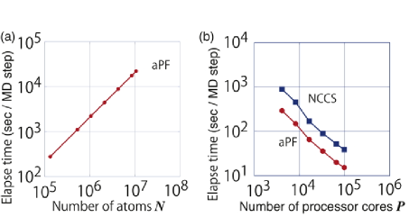
Figure 1: (a) Benchmark for the order-$N$ scaling. [5] (b) Benchmark for the parallel efficiency (strong scaling) with $10^{7}$ atoms on the K computer among $P$ = 4,096 - 98,304 processor cores. See the text for details.

In the present paper, the parallel efficiency is measured on the K computer for given materials with ten-million atoms. The resultant benchmark is called ‘strong scaling’ in the high-performance computation society. The numbers of the used processor cores are from $P=P_{\rm min}\equiv 4,096$ to $P=P_{\rm max}\equiv 98,304$. The MPI/OpenMP hierarchical parallelism was used and the parallel unit for the MPI or OpenMP parallelism is called ‘node’ or ‘thread’, respectively, throughout the present paper. The number of threads is fixed to be $P^{\rm(thread)}=8$, the maximum value on the K computer and the number of nodes is given by $P^{\rm(node)}=P/P^{\rm(thread)}=P/8$. The calculations were carried out in a couple of MD steps, with a TB-form Hamiltonian, [9] for amorphous-like conjugated polymer, poly-(9,9 dioctil-fluorene) (aPF) with $N$=10,629,120 atoms [5] and sp²-sp³ nano-composite carbon solid (NCCS) with $N$=10,321,920 atoms (See Ref. [10] for a related study).

As a result, a high parallel efficiency is found in Fig. 1 (b). The measure for the efficiency is obtained as $\alpha\equiv T(P_{\rm min})/T(P_{\rm max})\times(P_{\rm max}/P_{\rm min})=0.79$ or $\alpha=0.95$ for the aPF or NCCS case, respectively, where $T(P)$ is the elapse time with $P$ cores per MD step. In general, the elapse time increases with the increase of the number of orbitals per atom ($m_{\rm orb}$), as well as the number of atoms ($N$). The elapse time at the maximum cores is $T(P_{\rm max})$=39.1 sec for the NCC system and $T(P_{\rm max})$=15.3 sec for the aPF system, since the NCCS system has four (s- and p-type) orbitals per atom ($m_{\rm orb}=4$) and the aPF system contains hydrogen atoms with single (s-type) orbital and has, on average, only 2.3 orbitals per atom ($m_{\rm orb}=2.3$). The NCCS system was calculated also in a TB-form Hamiltonian with additional d orbitals ($m_{\rm orb}=9$). [11] The resultant elapse time is $T(P_{\rm max})$=311.0 sec and is larger than that without the d orbital ($T(P_{\rm max})$=39.1 sec), as should be.

Here several computational issues are discussed for (I) data-communication saving (II) memory-size saving and (III) parallel file reading/writing, since they are crucial for a high performance with practical computational resources. These issues affect the elapsed time and/or the required memory size but does not affect the resultant values of physical quantities. (I) The inter-node data communication is suppressed by the redundant calculation of several quantities, such as the matrix elements of $H$ and $S$, among the nodes. [5] (II) A workflow for the memory saving was built in the code and the workflow saves the required memory size drastically, at the sacrifice of a moderate increase of the time cost. In the memory-saving workflow, the data array for the Green’s function ($G$), the largest data array, is not stored in the memory but calculated twice redundantly, as follows:

$$(H,S)\Rightarrow G\Rightarrow\mu\Rightarrow({\rm 2nd\,calc.\,of\,}G)\Rightarrow\rho.$$ (3)

The first calculation of the Green’s function is carried out before the determination of the chemical potential $\mu$ in the bisection method. After that, the second calculation is carried out, since the density matrix $\rho$ is generated, as in Eq. (2), both from the Green’s function $G$ and the chemical potential $\mu$. In a result with $10^{5}$ atoms by a single-node workstation, the consumed memory size is reduced drastically from 28 GB in the non-memory-saving workflow into 1.6 GB in the memory-saving workflow, while the increase of the time is moderate (19 %). The reduction of the required memory is important, since the built-in memory size of the K computer is only 16 GB per node. All the calculations in Fig. 1 were carried out in the memory-saving workflow. (III) Out test calculation shows that the parallel file reading can give an important acceleration and was realized with split input files. A typical file size with $10^{7}$ atoms is one G byte (B) for our input atomic-structure data described in the extensible markup language (XML) format. [12] When the file with $N$ atoms is split into $n_{\rm split}$ files, each split file contains the data with approximately $N/n_{\rm split}$ atoms. The file writing is also parallelized, when each node saves the atomic structure data in the split XML format. As a result with 4,096 cores (512 nodes), the consumed time for the initial procedures $T_{\rm ini}$, or the procedures before starting the electronic structure calculation, is drastically reduced, from $T_{\rm ini}=1,423$ sec with the non-parallel file reading into $T_{\rm ini}=69$ sec with the parallel file reading. [13] The file writing procedure consumes a tiny time cost ( 0.2 - 0.4 sec). It is noteworthy that in most MD simulation studies, the file writing procedure of the atomic structure is carried out with a certain interval of MD steps, typically 10 steps. Therefore, the file writing time will be negligible in the whole simulation time.

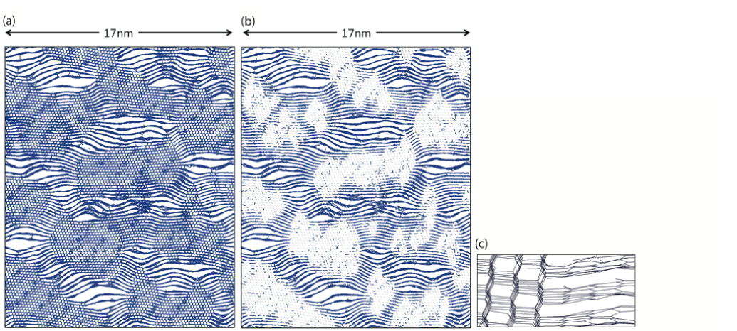
Figure 2: Bond visualization of sp²-sp³ nano-composite carbon solid (NCCS) with 10⁵ atoms by the COHP and $\pi$COHP analysis. The bonds are visualized both for the sp² and sp³ domains, or both for $\sigma$ and $\pi$ bonds in (a), while the bonds are visualized only for the sp² domain or for $\pi$ bonds in (b). A closeup of a sp²-sp³ domain boundary is shown in (c).

Now the discussion is turned into the second topic, the post-calculation analysis with huge electronic structure data.

The present paper presents analysis methods based on the Green’s function, i. e. crystalline orbital Hamiltonian population (COHP) method, [14] and its theoretical extension called $\pi$COHP method. The original COHP reveals the local bonding nature for each atom pair energetically and its definition is

$$C_{IJ}(\varepsilon)\equiv\frac{-1}{\pi}\sum_{\alpha,\beta}H_{J\beta;I\alpha}{\rm Im}\,G_{I\alpha;J\beta}(\varepsilon+{\rm i}0),$$ (4)

where the basis suffices, previously denoted by $i$ and $j$, are decomposed into the atom suffices, $I$ or $J$, and the orbital suffices, $\alpha$ or $\beta$ ($i\equiv(I,\alpha),j\equiv(J,\beta)$). The energy integration of COHP, called ICOHP, is also defined as

$$B_{IJ}\equiv\int f\left(\varepsilon-\mu\right)C_{IJ}(\varepsilon)d\varepsilon.$$ (5)

The sum of ICOHP gives the electronic structure energy or the sum of the occupied eigen levels; [14]

$$E_{\rm elec}\equiv\sum_{k}f(\varepsilon_{k}-\mu)\,\varepsilon_{k}=\sum_{I,J}B_{IJ}.$$ (6)

A large negative value of $B_{IJ}$ indicates the energy gain for the bond formation between the ($I,J$) atom pair. In the original paper, [14] the analysis is carried out for ab initio calculations in the linear-muffin-tin-orbital formulation [15]. The method was applied not only to insulator but also to metal, such as in Ref. [16]. The method is suitable for the present order-$N$ method, since the present method is based on the Green’s function. [17]

Here the $\pi$COHP is proposed as a theoretical extension of the original COHP. If the Hamiltonian contains the s- and p-type orbitals, for example, the off-site Hamiltonian term is decomposed into the $\sigma$ and $\pi$ components ($H_{J\beta;I\alpha}=H_{J\beta;I\alpha}^{(\sigma)}+H_{J\beta;I\alpha}^{(\pi)})$. The $\pi$COHP, $C_{IJ}^{(\pi)}$, will be defined in Eq. (4), when $H_{J\beta;I\alpha}$ is replaced by $H_{J\beta;I\alpha}^{(\pi)}$. The $\pi$ICOHP, $B_{IJ}^{(\pi)}$, will be defined in Eq. (5), when $C_{IJ}$ is replaced by $C_{IJ}^{(\pi)}$. The $\sigma$COHP, $C_{IJ}^{(\sigma)}$, and the $\sigma$ICOHP, $B_{IJ}^{(\sigma)}$, are defined in the same manners. From the definitions, the (I)COHP is decomposed into the sum of the $\sigma$(I)COHP and $\pi$(I)COHP

$$C_{IJ}(\varepsilon) = C_{IJ}^{(\sigma)}(\varepsilon)+C_{IJ}^{(\pi)}(\varepsilon)$$ (7)

$$B_{IJ} = B_{IJ}^{(\sigma)}+B_{IJ}^{(\pi)}.$$ (8)

Hereafter the original (I)COHP is called as ‘full’ (I)COHP. In the code, the full, $\sigma$ and $\pi$(I)COHP can be calculated automatically, without any additional data communication, during the massively parallelized order-$N$ calculation. One can distinguish the $\sigma$ and $\pi$ bonds, energetically, by the $\sigma$(I)COHP and $\pi$(I)COHP. A large negative value of $B_{IJ}^{(\sigma)}$ or $B_{IJ}^{(\pi)}$ indicates the $\sigma$ or $\pi$ bond formation between the atom pair, respectively.

In Fig. 2, the ($\pi$)COHP analysis is demonstrated in an NCCS system with 10⁵ atoms, so as to distinguish the sp² and sp³ domains, because one can distinguish the sp² domains from the sp³ domains by the presence of $\pi$ bonds. The system is a resultant structure of the our previous finite-temperature MD simulation with a periodic boundary condition. [10] The simulation is a preliminary research for the formation process of the nano-polycrystalline diamond (NPD), a novel ultra-hard materials. [18, 19] The NPD is produced directly from graphitic materials and consists of 10-nm-scale diamond-structure domains with a characteristic lamella-like structure. Its growth process is of great interest and possible precursor structures should be a ten-nm-scale composite between the sp² (graphite) and sp³ (diamond) domains. The present research is motivated from the above problem, though the present structures, still, have a gap in the length scale, when it is compared with experiments, as discussed later.

Figure 2 (a) or (b) shows the bond visualization with the full ICOHP or the $\pi$ICOHP, respectively. In Fig. 2(a), a bond is drawn for an $(I,J)$ atom pair, when its ICOHP value satisfy the condition of $B_{IJ}<B_{\rm th}$ with a given threshold value of $B_{\rm th}(<0)$. We found a typical value of $B_{\rm th}=-9$ eV. The visualization with the full ICOHP indicates the visualization both for sp² and sp³ bonds. In Fig. 2(b), on the other hand, a $\pi$ bond is drawn, when its $\pi$ ICOHP value satisfy the condition of $B_{IJ}^{(\pi)}<B_{\rm th}^{(\pi)}$ with a given threshold value of $B_{\rm th}^{(\pi)}(<0)$. We found a typical value of $B_{\rm th}^{(\pi)}=-1.5$ eV. The visualization with the $\pi$ICOHP indicates the visualization only for sp² bonds.

The bond visualization analysis in Figs. 2(a) and (b) concludes that the layered domains are sp² domains and the non-layered domains are sp³ domains. Figure 2(c) shows the visualization of a boundary region between sp² and sp³ domains. Here one can confirms that a layered domain form an sp² or graphite-like structure and a non-layered domain form an sp³ or diamond-like structure, as expected from the ($\pi$)ICOHP analysis.

Several points are discussed for the ($\pi$)COHP analysis. (I) The value of $|B_{\rm th}^{(\pi)}|$ is much smaller than that of $|B_{\rm th}|$, because the $\pi$ bonding is much weaker than the $\sigma$ bonding. (II) The threshold values for the bond visualizations, $B_{{\rm th}}$ and $B_{{\rm th}}^{(\pi)}$, may not be universal among materials but is independent on the system size. One should choose a typical value once for a material and can use the value among different system sizes. (III) One should be careful, sometimes, in the interpretation of the analysis result, because the $\pi$COHP analysis dose not detect an sp² bond but detects a contribution of the $\pi$-bonding component, as explained above. For example, the initial structure for the simulation of Fig. 2 contains defects among the sp³ domains, [10] as ‘seeds’ of the sp²-sp³ domain boundary. The resultant structure in Fig. 2 still has several initial defects in the sp³ domains and $\pi$ bonds are often drawn in Fig. 2(b) at such local defective regions. Such a $\pi$ bond does not mean an $sp^{2}$ bond. (IV) The structure of Fig. 2 has a gap in the length scale, when it is compared with experiments. The structure is a ‘2D-like’ one, because the periodic cell length in the perpendicular direction to the paper (2nm) is much smaller than the other two cell lengths, 17 nm or more. [10] The artificial ‘2D-like’ situation affect severely the resultant atomic structure and makes a difficulty for a direct comparison between the simulation and experiment. A more realistic situation with the ten-nanometer simulation cell sizes in the three directions requires million-atom MD simulation, ten times larger than that in the present result. [10] Such a larger MD simulation may be a possible target in near future with the parallel computations. (V) The bond visualization of Figs. 2(a)-(c) was realized by our original visualization tool ’VisBAR’(=Visualization tool with Ball, Arrow and Rods). The tool is based on Python (www.python.org) and was developed for our needs in the large-scale calculations, like the ($\pi$)COHP analysis.

In summary, (i) a high parallel efficiency was found in ten-million-atom order-$N$ electronic structure calculations on the K computer with approximately $10^{5}$ processor cores. Important computational issues are addressed for communication, memory size and file reading/writing. (ii) The ($\pi$) COHP analysis method is presented as a practical post-calculation analysis method ideal for the huge distributed data of the Green’s function. The analysis is demonstrated in a sp²-sp³ nano-composite carbon solid, so as to distinguish sp² and sp³ domains. The example shows a typical need of large-scale electronic structure calculation that requires both large-scale calculation and large-data analysis with huge distributed data.

The present research indicates general aspects of computational physics, beyond electronic structure calculation, with current or next-generation supercomputers. Numerical algorithm and computer scientific methods will be inseparable from physics. A physical discussion should be constructed from physical quantities, like the Green’s function or the ($\pi$-)COHP, that can be computed, analyzed and visualized with massively parallel computer architectures. All the methods discussed here, ones for calculation, parallel file reading/writing with split XML file, memory saving workflow, post-calculation data analysis, and visualization, are designed to be suitable for the massively parallel computer architecture, and some of them may be useful in other computational physics fields.

Acknowledgments The present research is partially supported by the Field 4 ( Industrial Innovation ) of the HPCI Strategic Program of Japan. A part of the results is obtained by the K computer at the RIKEN Advanced Institute for Computational Science (The early access and the proposal numbers of hp120170, hp120280). This research is supported partially by Grant-in-Aid for Scientific Research (No. 23104509, 23540370) from the Ministry of Education, Culture, Sports, Science and Technology (MEXT) of Japan. This research is supported also partially by Initiative on Promotion of Supercomputing for Young Researchers, Supercomputing Division, Information Technology Center, The University of Tokyo. The supercomputers were used also at the Institute for Solid State Physics, University of Tokyo and at the Research Center for Computational Science, Okazaki.

References

- [1] H. Teng, T. Fujiwara, T. Hoshi, T. Sogabe, S.-L. Zhang and S. Yamamoto, Phys. Rev. B 83 (2011) 165103.
- [2] T. Sogabe and S.-L. Zhang, International Conference on Numerical Analysis and Scientific Computing with Applications, Agadir, Morocco, 2009.
- [3] T. Sogabe, T. Hoshi, S.-L. Zhang, T. Fujiwara, J. Comp. Phys. 231 (2012) 5669.
- [4] T. Yamashita, T. Miyata, T. Sogabe, T. Fujiwara, S.-L. Zhang, Trans. JSIAM 21 (2011) 24. [in Japanese]
- [5] T. Hoshi, S. Yamamoto, T. Fujiwara, T. Sogabe, S.-L. Zhang, J. Phys.: Condens. Matter 21 (2012) 165502.
- [6] A. Frommer, Computing 70, (2003) 87.
- [7] S. Yamamoto, T. Fujiwara and Y. Hatsugai, Phys. Rev. B 76 (2007) 165114; S. Yamamoto, T. Sogabe, T. Hoshi, S.-L. Zhang, and T. Fujiwara, J. Phys. Soc. Jpn. 77 (2008) 114713.
- [8] M. Elstner, D. Porezag, G. Jungnickel, J. Elsner, M. Haugk, Th. Frauenheim, S. Suhai and G.Seifert G, Phys. Rev. B 58 (1998) 7260.
- [9] G. Calzaferri and R. Rytz, J. Phys. Chem. 100 (1996) 11122.
- [10] T. Hoshi, T. Iitaka, M. Fyta, J. Phys.: Conf. Ser. 215 (2010) 012118.
- [11] J. Cerdá and F. Soria, Phys. Rev. B 61 (2000) 7965.
- [12] Since the atomic structure data requires three () components in the double precision (8B) value for each atom, the required data size with (=10M) atoms is estimated to be M = 240 MB.
- [13] The consumed time only for the file reading can not be measured, since other procedures, such as array allocation and calculations, are carried out during the file reading,
- [14] R. Dronskowski and P. E. Blöchl: J. Phys. Chem. 97 (1993) 8617.
- [15] O. K. Andersen and O. Jepsen, Phys. Rev. Lett. 53 (1984) 2571.
- [16] Y. Ishii and T. Fujiwara, J. of Non-Crys. Sol. 334&335 (2004) 336.
- [17] R. Takayama, T. Hoshi and T. Fujiwara, J. Phys. Soc. Jpn. 73 (2004) 1519; R. Takayama, T. Hoshi, T. Sogabe, S.-L. Zhang and T. Fujiwara Phys. Rev. B 73 (2006) 165108.
- [18] T. Irifune, A. Kurio, A. Sakamoto, T. Inoue and H. Sumiya, Nature 421 (2003) 599.
- [19] C. L. Guillou, F. Brunet, T. Irifune, H. Ohfuji and J.-N. Rouzaud Carbon 45 (2007) 636.