Revisiting the derivation of spin precession effects in quasi one-dimensional quantum wire models

Abstract

In this paper one deals with the theoretical derivation of spin precession effects in quasi 1D quantum wire models. Such models get characterized by equal coupling strength superpositions of Rashba and Dresselhaus spin-orbit interactions of dimensionless magnitude $a$ under the influence of in-plane magnetic fields of magnitude $B$. Besides the wavenumber $k$ relying on the 1D electron, one accounts for the $s=\pm$ $1$ - factors in the front of the square root term of the energy. Electronic structure properties of quasi 1D semiconductor heterostructures like InAs quantum wires can then be readily discussed. Indeed, resorting to the 2D rotation matrix provided by competing displacements working along the Ox-axis opens the way to derive precession angles one looks for, as shown recently. Proceeding further, we have to resort reasonably to some extra conditions concerning the general selection of the $k$-wavenumber via $kL=1$, where $L$ stands for the nanometer length scale of the quantum wire. We shall also account for rescaled wavenumbers, which opens the way to extrapolations towards imaginary and complex realizations. The parameter dependence of the precession angles is characterized, in general, by interplays between admissible and forbidden regions, but large monotony intervals are also in order.

I INTRODUCTION

Spin-orbit interactions which are present in quasi one-dimensional (1D) semiconductor heterostructures like $InAs$ quantum wires provide a promising way to controllable spin manipulations1 . Besides the Rashba spin-orbit interaction $V_{R}=\alpha_{R}\left(\sigma_{x}p_{y}-\sigma_{y}p_{x}\right)/\hbar$  2 , which is induced by an electric field, one deals with the linearized Dresselhaus spin-orbit interaction $V_{D}=\alpha_{D}\left(\sigma_{x}p_{x}-\sigma_{y}p_{y}\right)/\hbar$  3 . These interactions rely on the presence of a structural and crystal inversion symmetry, respectively. Superpositions of such interactions under the influence of transversal4 and in-plane magnetic fields5 ; 6 like $\overrightarrow{B}=B(\cos\theta,\sin\theta)$, have also been discussed. The polar angle between the magnetic field and the $Ox$-axis is denoted by $\theta$. The corresponding couplings are denoted by $\alpha_{R}$ and $\alpha_{D}$, in which case the equal coupling strength regime7 ; 8 proceeds via $\alpha_{0}=\alpha_{R}=\pm\alpha_{D}$. A typical choice is given by $\alpha_{R}=2\times 10^{-11}eVm$, or equivalently, $a=1$, where $a=(\alpha_{0}/2)\times 10^{11}/eVm$ denotes the dimensionless spin-orbit coupling. Equal coupling strength superpositions of such interactions in the presence of in-plane magnetic fields have also been analyzed recently9 . In this later case it has been shown that accounting for spin conservations amounts to the selection of the polar angle along the bisectrices. Having obtained the energy band opens the way to the theoretical derivation of novel spin precession effects, as shown by (72) in Ref. 9. For this purpose one proceeds along the lines presented before10 , but now by resorting to a different energy band structure. This amounts to reverse the usual $k$-wavenumber dependence of the energy in order to establish two correlated wavenumbers, say $k_{+}$ and $k_{-}$, which are responsible for the description of propagation paths along the $Ox$-axis. Then the two dimensional rotation matrix11 one looks for can be established in terms of displacements of length $L$ acting along the two paths just referred to above9 ; 10 . However, several details referring to a systematic study of the parameter dependent spin precession angles are still desirable. The suitable selection of the $k$-parameter deserves a little bit more attention, too. Besides the influence of the discrete parameter $s=\pm 1$, which is responsible for the $\pm$-signs in the front of the square root of the energy, we shall account this time for a further parameter, say $K$, reflecting the rescaling of squared wavenumber via $k^{2}\rightarrow Kk^{2}$. Handling the parameter dependence of spin precession angles established in this manner amounts to deal with interplays between $k$, $B$, $a$, $s$ and $K$, which represents our main motivation in this paper. So far numerical $k$-inputs are introduced via $kL=1$, where $L$ denotes specifically the nanometer length scale of the quantum wire model. Forbidden regions can be readily established in terms of selected parameters for which the precession angles are imaginary. This happens in configurations for which $s=-1$. Complementary intervals should then be responsible for admissible configurations. The $K$-parameter opens the way to extrapolations of the wavenumber towards imaginary and complex values, which looks promising for further generalizations.

The paper is organized as follows. Preliminaries and notations are discussed in Sec. II. The present Hamiltonian is introduced by neglecting, for convenience, the orbital effects of the magnetic field. Accounting for spin conservations leads to the selection of   two $\theta$-angles, namely of $\theta=\pi/4$ and $\theta=3\pi/4,$ in which case $\alpha_{R}=\alpha_{D}$ and $\alpha_{R}=-\alpha_{D}$ , respectively. Then the equal strength limit of the energy can be readily established. This leads in turn to the displacement momenta $k=$ $k_{\pm}$ serving to the description of two paths one looks for, as indicated in Sec. III. In Sec. IV one shows that such momenta work safely whenever $s=1$, but suitable convergence conditions have to be accounted for in so far as $s=-1$. Precession angles established before to first $\varepsilon$-order via $\Theta=(k_{+}-k_{-})L$ are discussed in Sec. V. Numerical studies concerning these angles are presented in some detail in Sec. VI. Section VII deals with imaginary and complex realizations of the $k$-parameter. The Conclusions are presented in Sec. VIII. Mathematical details concerning the derivation of precession angles are shortly reviewed in the Appendix.

II PRELIMINARIES AND NOTATIONS

In order to perform the quantum theoretical description of electronic behavior in two-dimensional (2D) semiconductor heterostructures, single particle Hamiltonians5 ; 6

$$H_{tot}=\frac{p_{x}^{2}+p_{y}^{2}}{2m^{\ast}}+V_{R}+V_{D}+V_{Z}+V\left(y\right)$$ (1)

including the spin-orbit interactions have been proposed. This time the orbital effects of the magnetic field have been neglected. The momentum operator reads $\overrightarrow{p}=-i\hbar\nabla$, whereas $m^{\ast}$ stands for the effective mass of the electron. One has e.g. $m^{\ast}=0.04m_{0}$ for $InAs$ quantum wires12 , where $m_{0}$ denotes the usual rest-mass of the electron. The wire geometry is characterized by a transversal confining potential, say $V\left(y\right)=m^{\ast}\omega_{0}^{2}y^{2}/2$. The Zeeman interaction $V_{Z}=\mu_{B}\left(\sigma_{x}B_{x}+\sigma_{y}B_{y}\right)g/2$ has also been incorporated, where $\mu_{B}=e\hbar/2m_{0}c$ stands for the Bohr-magneton, while $g$ denotes the effective gyromagnetic factor. For convenience, we shall assume that $g=2$, as usual.

Using the total Hamiltonian displayed in (1) leads to commutation relations like

$$\left[H_{tot},\sigma_{x}\mp\sigma_{y}\right]=\frac{2i\sigma_{z}}{\hbar}\left(p_{x}\pm p_{y}\right)\left(\alpha_{R}\pm\alpha_{D}\right)-i\sigma_{z}g\mu_{B}B\left(\sin\theta\mp\cos\theta\right)\quad$$ (2)

which exhibit the zero value if

$$\alpha_{R}=\mp\alpha_{D}\text{\qquad and\qquad}\tan\theta=\pm 1\quad.$$ (3)

So, one gets faced with conserved spin observables like $\sigma_{x}+\sigma_{y}$ and $\sigma_{x}-\sigma_{y}$ when the Rashba and Dresselhaus couplings exhibit the same magnitude, i.e. $\alpha_{R}=-\alpha_{D}$ and $\alpha_{R}=\alpha_{D},$ respectively. This proceeds in conjunction with selected in-plane orientations of the magnetic field $\overrightarrow{B}$ for which $\tan\theta=1$ and $\tan\theta=-1$, respectively, as displayed above.

The energy eigenvalue problem can be solved by resorting once more again to the zero determinant condition for a homogenous system of two coupled equations, as shown many times before13 ; 14 ; 15 . Starting from the wavefunction

$$\Psi(x,y)=\exp(ikx)\Phi_{n}(y)\binom{\psi_{1}}{\psi_{2}}\quad$$ (4)

where $\Phi_{n}(y)$ stands for the oscillator eigenfunction, yields the 1D-reduction of (1) as

$$H_{1}=\frac{p_{x}^{2}}{2m^{\ast}}-\left(\alpha_{R}\sigma_{y}-\alpha_{D}\sigma_{x}\right)\frac{p_{x}}{\hbar}+\frac{g}{2}\mu_{B}B(\sigma_{x}\cos\theta+\sigma_{y}\sin\theta)+E_{n}^{0}\quad$$ (5)

in which the oscillator eigenvalue reads $E_{n}^{0}=\hbar\omega_{0}(n+1/2)$, as usual (see e.g.Ref. [13]). Now we are ready to apply the zero determinant condition referred to above, which produces the energy

$$E=E_{n}^{(\pm)}(\theta)=\frac{\hbar^{2}k^{2}}{2m^{\ast}}+E_{n}^{0}\pm\sqrt{\Omega}$$ (6)

in accord with (16) in16 , where

$$\Omega=k^{2}(\alpha_{R}^{2}+\alpha_{D}^{2})+kg\mu_{B}B\left(\alpha_{D}\cos\theta-\alpha_{R}\sin\theta\right)+\left(\frac{g}{2}\mu_{B}B\right)^{2}\quad.$$ (7)

and where the $\pm$-signs in the front of $\sqrt{\Omega}$ can also be viewed, in general, as reflecting the influence of the spin16 ; 17 . We then have to introduce a further parameter like $s=\pm 1$, which will be used hereafter. Accordingly, the lower energy configuration corresponds to $s=-1$.

The corresponding spinorial eigenfunction is given by $\psi_{1}=1/\sqrt{2}$ and $\psi_{2}=\pm\exp(-i\beta)/\sqrt{2}$, where

$$\tan\beta=\frac{k\alpha_{R}-(g/2)\mu_{B}B\sin\theta}{k\alpha_{D}+(g/2)\mu_{B}B\cos\theta}\quad.$$ (8)

The equal strength limit of (8) can also be readily performed. One would then obtain $\tan\beta=-\tan\theta$, in accord with (3), so that $\beta=\pi-\theta$. This means that $\beta=\pi/4$ $(3\pi/4)$ if $\alpha_{R}=\alpha_{D}$ $(\alpha_{R}=-\alpha_{D})$.

Accounting for the spin conservation, we have to realize that the symmetrized equal coupling strength limit of the present spin dependent but non-symmetrized energy band (6) is given by

$$E_{n}^{(s)}(B,a)=\frac{\hbar^{2}k^{2}}{2m^{\ast}}+E_{n}^{0}+\frac{s}{2}\sqrt{8k^{2}\alpha_{0}^{2}+\left(g\mu_{B}B\right)^{2}}$$ (9)

by virtue of (3). So far, the dimensionless spin-orbit coupling, i.e. $a=(\alpha_{0}/2)\times 10^{11}/eVm$ , has the magnitude order of unity. One sees that the linear $B$-dependent term under the square root in (6) is ruled out, which comes definitely from the inter-related equal coupling strength limit one deals with in this paper. Moreover, ruling out the $B$-dependent term leads to the conversion of (6) into a conditionally solvable biquadratic equation in $k^{2}$, which serves as a starting point to the derivation of spin precession effects.

Rescaled variables like $\widetilde{\alpha}_{0}=m^{\ast}\alpha_{0}/\hbar^{2}$, $\widetilde{B}=m^{\ast}B/\hbar^{2}$, $E_{n}^{(s)}(B,\alpha_{0})=\hbar^{2}\xi^{2}/2m^{\ast}$ and $E_{n}^{0}=\hbar^{2}\kappa_{n}^{2}/2m^{\ast}$ can also be introduced. Numerical studies can then be readily done by starting from $m^{\ast}/\hbar^{2}\cong 5.24936\times 10^{17}/eVm^{2}$, $g\mu_{B}\cong 1.157668\times 10^{-4}eV/T$, $g\mu_{B}m^{\ast}/\hbar^{2}\cong 6.077016\times 10^{13}/m^{2}T$ , $\widetilde{\alpha}_{0}\cong 1.049872a\times 10^{7}/m$ and $n=0$. We shall also assume that $E_{0}^{0}=1meV$  13 . We have to keep in mind that present calculations are sensitive to the numerical selection of $k$-parameter. We have to realize that such selections can be established reasonably via$\ kL=1$, which yields a typical nanometer length like $L=10^{-7}m$, when $k=10^{7}/m$. However, we have to be aware that other selections, $k$-dependent ones included, are conceivable. For convenience, we shall insert hereafter the wavenumber input $k=10^{7}/m$, though the choice $k=10^{8}/m$ has been used tentatively before9 .

III INVERTING THE WAVENUMBER DEPENDENCE OF THE ENERGY

It is also clear that (9) can be rewritten equivalently as

$$\xi^{2}-\kappa_{n}^{2}=A_{s}(B,\alpha_{0},k)=A_{\pm}(B,\alpha_{0},k)\equiv k^{2}+s\left[8k^{2}\widetilde{\alpha}_{0}^{2}+(g\mu_{B}\widetilde{B})^{2}\right]^{1/2}$$ (10)

where $s=\pm 1$, which produces the factorized algebraic equation

$$k^{4}-2(A_{\pm}+4\widetilde{\alpha}_{0}^{2})k^{2}+A_{\pm}^{2}-(g\mu_{B}\widetilde{B})^{2}=(k^{2}-k_{+}^{2})(k^{2}-k_{-}^{2})$$ (11)

where $k^{2}=k_{\pm}^{2}$ stand implicitly for the roots serving to the description of two propagation paths. Next we shall resort to a further approximation, namely to handle in the sequel the $A_{\pm}$-functions in terms of numerical inputs for the $k$-parameter. Then we are in a position to establish actually $k$-roots one looks for as

$$k=k_{\pm}=\Omega_{0}\sqrt{1\pm\varepsilon}$$ (12)

where

$$\varepsilon=\frac{\left[8\widetilde{\alpha}_{0}^{2}A_{\pm}+16\widetilde{\alpha}_{0}^{4}+(g\mu_{B}\widetilde{B})^{2}\right]^{1/2}}{\Omega_{0}^{2}}>0$$ (13)

and

$$\Omega_{0}=\left(4\widetilde{\alpha}_{0}^{2}+A_{\pm}\right)^{1/2}\quad.$$ (14)

The same job can be done by resorting to numerical energy-inputs, such as indicated by the equation

$$E_{n}^{(1)}+E_{n}^{(-1)}-2E_{n}^{0}=\frac{\hbar^{2}k^{2}}{m^{\ast}}\quad.\qquad$$ (15)

Accordingly, one obtains $k=10^{7}/m$ when $E_{0}^{(1)}+E_{0}^{(-1)}=2.1905meV$.

IV CONVERGENCE CONDITIONS

One remarks that (12) produces a power series in terms of the convergence condition $\varepsilon^{2}<1$, which is synonymous to

$$g\mu_{B}\mid\widetilde{B}\mid<\mid A_{\pm}\mid\quad.$$ (16)

This inequality is fulfilled automatically if $s=1$. However one gets faced with extra conditions like

$$8\widetilde{\alpha}_{0}^{2}-k^{2}>2g\mu_{B}\mid\widetilde{B}\mid>0$$ (17)

if $s=-1$, provided that

$$8\widetilde{\alpha}_{0}^{2}>k^{2}\quad.$$ (18)

Next, we shall handle (17) via $8\widetilde{\alpha}_{0}^{2}=0(1)$, $2g\mu_{B}\mid\widetilde{B}\mid=0(1)$ and $k^{2}=0(\epsilon)$, where $\epsilon$ stands for a small parameter. Such conditions are reminiscent to the asymptotic description of nonlinear oscillations18 . The interesting point is that (17) provides an admissible but finite $B$-interval such as given by

$$B\in I_{B}(a)=\left(-B_{c}a^{2},B_{c}a^{2}\right)$$ (19)

in so far as the $k^{2}$-term is neglected, where

$$B_{c}=\frac{16m^{\ast}}{g\mu_{B}\hbar^{2}}10^{-22}T\quad.$$ (20)

It should be noted that $a$ plays this time the role of an input parameter. Conversely, starting from an input $B$-parameter leads to two disjoint but admissible semi-infinite $a$-intervals like

$$\widetilde{I}_{a}^{(-)}(B)=\left(-\infty,-\sqrt{\frac{B}{B_{c}}}\right)$$ (21)

and

$$\widetilde{I}_{a}^{(+)}(B)=\left(\sqrt{\frac{B}{B_{c}}},\infty\right)$$ (22)

so that (18) gets converted into

$$a\in\widetilde{I}_{a}(B)=\widetilde{I}_{a}^{(-)}(B)\cup\widetilde{I}_{a}^{(+)}(B)\quad.$$ (23)

Concrete realizations concerning (19) and (23) will be presented below.

Under such conditions the leading approximations characterizing (12) are given by

$$k=k_{\pm}=\Omega_{0}\left(1\pm\frac{\varepsilon}{2}\right)=\Omega_{0}\pm\Omega_{1}$$ (24)

both for $s=1$ and $s=-1$, where $\Omega_{1}=\varepsilon\Omega_{0}/2$, with the understanding that in the latter case the wavenumber description proceeds in terms of (19) and (23).

V SPIN PRECESSION EFFECTS

Displacements of length $L$ along the $Ox$-axis can be readily applied by resorting to the orthonormalized spinor

$$\left|\Psi_{\pm}\right\rangle=\frac{1}{\sqrt{2}}\left(\begin{array}[]{c}1\\ \pm\exp\left(-i\beta\right)\end{array}\right)$$ (25)

by virtue of (4). This results in a 2D rotation matrix [10,11], providing in turn the precession angle as

$$\Theta(B,a;s)=2\Omega_{1}L=\frac{\alpha_{0}m^{\ast}L}{\hbar^{2}}\left[\frac{16\alpha_{0}^{2}\left(m^{\ast}/\hbar^{2}\right)^{2}+\left(g\mu_{B}B/\alpha_{0}\right)^{2}+8A_{\pm}}{4\alpha_{0}^{2}\left(m^{\ast}/\hbar^{2}\right)^{2}+A_{\pm}}\right]^{1/2}$$ (26)

as shown in the Appendix, which proceeds in accord with (72) in Ref. 9. Our main emphasis in this paper is one Refs. 9 and 10, but we have to mention that starting with the idea of the voltage controlled spin precession19 , a multitude of spin precession descriptions have also been presented during time20 ; 21 ; 22 ; 23 ; 24 , numerical studies included25 ; 26 .

Now we are ready to discuss the parameter dependence of the precession angle in a more systematic manner. Inserting $k=10^{7}/m$ , provides in turn the $B$- and $a$-dependence of the precession angle $\Theta(B,a;s)$ in terms of $a$- and $B$-inputs respectively. One finds that $\Theta(B,a;s)$ is a positive concave function  of $B$ and $a$ increasing monotonically with $\mid B\mid$ and $\mid a\mid$, respectively, in so far as $s=1$. However, one gets faced with nontrivial patterns when $s=-1$. So there are crossing points between $\Theta$-plots for $s=1$ and $s=-1$ concerning both $B$- and $a$-dependent curves. Such points are located at

$$B=B_{\pm}(a)=\pm B_{c}a^{2}$$ (27)

and

$$a=a_{\pm}(B)=\pm\sqrt{\frac{B}{B_{c}}}$$ (28)

respectively. These points reproduce identically the edge points characterizing the admissible intervals (19) and (23). It should be noted that both (27) and (28) are produced by the basic equation

$$(g\mu_{B}\widetilde{B})^{2}=16\widetilde{\alpha}_{0}^{4}$$ (29)

which has the meaning of a leading approximation. The upper bounds characterizing the precession angle within the admissible intervals are then given by

$$\Theta=\Theta_{1}(a)=\Theta(B_{\pm}(a),a;s=-1)=2.099744\sqrt{2}a$$ (30)

and

$$\Theta=\Theta_{2}(B)=\Theta(B,a_{\pm}(B);s=-1)=2.099744\sqrt{\frac{2B}{B_{c}}}$$ (31)

where $a$ and $B$ stand for inputs. Other characteristic point of interest are the zeros exhibited by the $s=-1$-precession angle on the $B$- and $a$-axes. One realizes that such zeros are inter-related with the onset of discontinuity points of  the second kind such that $\Re\Theta(B,a;s=-1)=0$, as displayed in Figs. 1-4. Handling this latter equation gives

$$k^{2}+\sqrt{k^{4}+(g\mu_{B}\widetilde{B})^{2}}=4\widetilde{\alpha}_{0}^{2}$$ (32)

which yields the solutions

$$B=B_{\pm}^{(0)}(a)=\pm\frac{2\sqrt{2}\widetilde{\alpha}_{0}}{g\mu_{B}m^{\ast}/\hbar^{2}}\sqrt{2\widetilde{\alpha}_{0}^{2}-k^{2}}\in I_{B}(a)$$ (33)

or

$$a=a_{\pm}^{(0)}(B)=\pm\frac{\hbar^{2}}{4m^{\ast}}\left[k^{2}+\left[k^{4}+(g\mu_{B}\widetilde{B})^{2}\right]^{1/2}\right]^{1/2}\in\widetilde{I}_{a}(B)$$ (34)

respectively. It can be easily verified that the zeros established in this manner get included into the admissible intervals (19) and (23). We have to remark that the that the zeros of the denominator in (31) such as given by

$$(g\mu_{B}\widetilde{B})^{2}=16\widetilde{\alpha}_{0}^{4}+k^{4}$$ (35)

produce vertical singularity lines which are asymptotically indistinguishable from supercritical $\Theta$-tails for which $\Theta(B,a;s=-1)\eqslantgtr\Theta_{1}$ and $\Theta(B,a;s=-1)\eqslantgtr\Theta_{2}$, which proceed in connection with $B=B_{\pm}(a)$ and $a=a_{\pm}(B)$, respectively. The understanding is that (29) is a leading approximation which comes from (35) via $k^{2}\rightarrow 0$. Such vanishingly small strips tails lying outside admissible regions should then be viewed as meaningless artifacts which can be hereafter ignored. Under such conditions one gets faced with a leading approximation for which $\Theta(B,a;s=1)\eqslantgtr\Re\Theta(B,a;s=-1)$, which opens the way to a reasonable synthesis of admissible $\Theta$-trajectories in pertinent parameter spaces.

After having been arrived at this stage, we are in a position to say that forbidden regions should proceed complementarily in terms of selected parameters for which the imaginary parts of precession angles are non-zero, i.e. for $\Im\Theta(B,a;s=-1)\neq 0$. It is understood that this latter inequality proceeds in combination with $\Re\Theta(B,a;s=-1)=0$. Such parameters belong to intervals like

$$C_{B}(a)=(-\infty,B_{-}(a))\cup(B_{+}(a),\infty)$$ (36)

and

$$\widetilde{C}_{a}(B)=(a_{-}(B),a_{+}(B))$$ (37)

which are complementary to (19) and (23), respectively.

VI NUMERICAL STUDIES

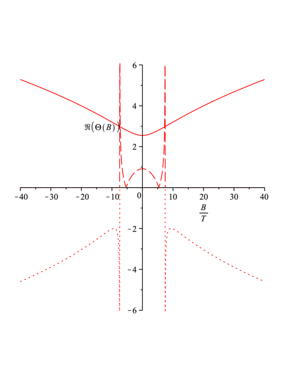
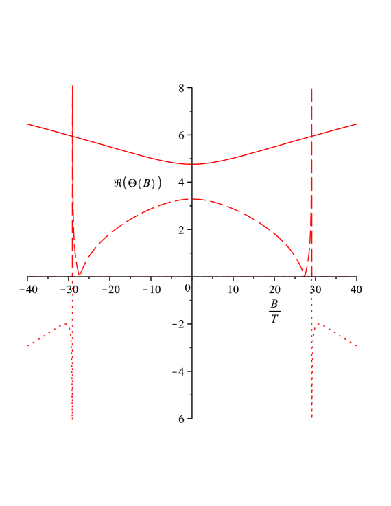
Concrete plots displaying the parameter dependence of precession angles are presented in Figs. 1-4. We have to anticipate that in all these cases the precession angles are positive whenever $s=1$. The precession angle is presented in Fig. 1 for $a=1$, $s=1$ (solid curve) and $s=-1$ (dashed curve). The crossing points are located at $B_{\pm}(1)=\pm B_{c}\cong\pm 7.255082T$, while the zeros are given by $B_{\pm}^{(0)}(1)\cong\pm 5.363195T$. The admissible $B$-interval is given by $I_{B}(1)$, while the forbidden one proceeds via $C_{B}(1)$, in accord with the dotted curve in Fig. 1. The horizontal and vertical dotted lines serve to the discrimination of crossing points, and the same concerns Figs. 2-4. Inserting $a=2$ instead of $a=1$ leads to similar patterns, as shown in Fig. 2. The crossing points and the zeros are now given by $B_{\pm}(2)\cong 29.020328T$ and $B_{\pm}^{(0)}(2)\cong 27.326675T$, respectively. The admissible interval concerns this time $I_{B}(2)$, which is complementary to the forbidden interval $C_{B}(2)$ in which $\Im\Theta(B,2;s=-1)\neq 0$.

Figure 1: The $B$-dependence of the real parts of precession angles for $a=1$, $s=1$ (solid curve) and $s=-1$(dashed curve). Dotted curves displaying the $B$-dependence of $\Im\Theta(B,a=1;s=-1)$ have also been inserted.

Figure 2: The $B$-dependence of the real parts of precession angles for $a=2$, $s=1$ (solid curve) and $s=-1$(dashed curve). Now the dotted curves concern the $B$-dependence of $\Im\Theta(B,a=2;s=-1)$.

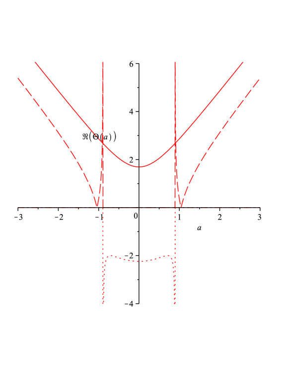
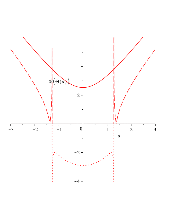
The $a$-dependence of the precession angle can be discussed in a rather similar manner. Inserting $B=6T$, leads to typical plots for $s=1$ (solid curves) and $s=-1$ (dashed curves), which exhibit the crossing points $a_{\pm}(6)\cong\pm 0.827006$ and the zeros $a_{\pm}^{(0)}(6)\cong\pm 1.041294$, as shown in Fig. 3. However, this time the admissible interval is expressed by two disjoint semi-infinite intervals, i.e. by $\widetilde{I}_{a}(6)$. The dotted curve concerns this time the forbidden interval $\widetilde{C}_{a}(6)$. The $B=12T$- counterparts of these plots are displayed in Fig. 4. Just note that in this latter case crossing points and zeros are given by $a_{\pm}(12)\cong\pm 1.286084$ and $a_{\pm}^{(0)}(12)\cong\pm 1.377026$.

Figure 3: The $a$-dependence of the real parts of precession angles for $B=6T$, $s=1$ (solid curve) and $s=-1$ (dashed curve). The $a$-dependence of $\Im\Theta(B=6,a;s=-1)$ is displayed by the dotted curve.

Figure 4: The $a$-dependence of the real parts of precession angles for $B=12T$, $s=1$ (solid curve) and $s=-1$ (dashed curve). Now the dotted curve is responsible for the $a$-dependence of $\Im\Theta(B=12,a;s=-1)$.

VII THE INFLUENCE OF IMAGINARY AND COMPLEX WAVENUMBERS

Next let us rescale the squared wavenumber as

$$k^{2}\rightarrow k_{R}^{2}=Kk^{2}$$ (38)

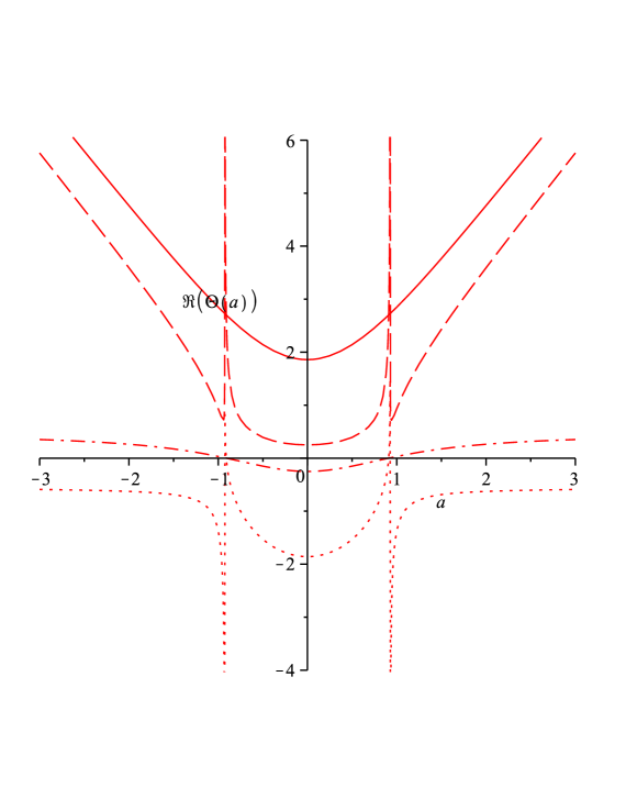
which means that imaginary $k-$realizations proceed via $K<0$. The $K$-dependence of $\Theta=\Theta(B,a;s,K)$ can be easily displayed, as shown in Fig. 5 for $B=6T$ and $a=1$. One remarks that the imaginary parts of precession angles, such as indicated by dot-dashed ($s=1$) and dotted ($s=-1$) curves, are zero, unless $K<K_{c}$, where $K_{c}\cong-1.51$. Correspondingly, the real parts of present $\Theta$-angles, which are displayed by solid ($s=1$) and dashed ($s=-1$) curves, get characterized by a discontinuity point of second kind for which $\Re\Theta(6,1;s=\pm 1,K_{c})$ $\cong 2.549063$. The imaginary and real parts obey the symmetry properties

$$\Im(\Theta(6,1;s=1,K)+\Theta(6,1;s=-1,K))=0$$ (39)

which is valid irrespective of $K$ and

$$\Re\Theta(6,1;s=1,K)=\Re\Theta(6,1;s=-1,K)$$ (40)

working for $K\eqslantless K_{c}$. A further discontinuity point of second kind is located at $K=K_{1}\cong 0.692018$, such that $\Theta(6,1;s=-1,K_{1})=0$, which is similar to the zeros displayed by $\Re\Theta(B,a;s=-1,K=1)$ in Figs. 1-4.

Figure 5: The $K$-dependence of the real parts of precession angles for $B=6T$, $a=1$, $s=1$ (solid curve) and $s=-1$ (dashed curve). The $K$-dependence of $\Im\Theta(B=6,a=1;s=\pm 1,K)$  has also been included, as shown by dot-dashed ($s=1$) and dotted ($s=-1$) curves.

A further interesting example concerns the $a$-dependence of real parts of precession angles for $B=6T$ and $K=i$, as shown by solid ($s=1$) and dashed ($s=-1$) curves in Fig. 6. Dot-dashed ($s=1$) and dotted ($s=-1$) curves, which are responsible for the imaginary parts, have again been inserted. It is clear that now the rescaled wavenumber exhibits the complex form $k_{R}=\exp(i\pi/4)k$. Just remark the symmetry of present numerical realizations such as given by

$$\Theta(B=6,a=0;s=1,K=i)=1.858427-i0.250224$$ (41)

and

$$\Theta(B=6,a=0;s=-1,K=i)=-i1.858427+0.250224$$ (42)

Vertical asymptotes reflecting the influence of crossing points $a=a_{\pm}(B=6)\cong 0.909399$ discussed before by virtue of (23) can also be readily identified. The present patterns are similar to the ones displayed in Fig. 4, but now one deals with additional imaginary contributions concerning $\Im\Theta(B=6,a;s=1,K=i)$ as well as $\Im\Theta(B=6,a;s=-1,K=i)$, this time for $a\in\widetilde{I}_{a}(B=6)$.

Figure 6: The $a$-dependence of real parts of precession angles for $B=6T$, $s=1$ (solid curve), $s=-1$ (dashed curves) and $K=i$. The $a$-dependence of $\Im\Theta(B=6,a;s=\pm 1,K=i$ ) has also been inserted, as shown by dot-dashed ($s=1$) and dotted ($s=-1$) curves.

VIII CONCLUSIONS

In this paper the parameter dependence of novel spin-precession effects proposed before9 has been discussed in some more detail. Such effects concern equal coupling strength combinations of Rashba and Dresselhaus spin-orbit interactions characterized by the dimensionless coupling $a$ under the influence of in-plane magnetic fields of magnitude $B$. The Zeeman interaction has been favoured to the detriment of the orbital effects of the magnetic field6 . A related discrete parameter, say $s=\pm 1$, has also accounted for. The spin precession angle has been derived in terms of suitable $\varepsilon$-expansions proceeding in terms of the convergence condition $\varepsilon^{2}<1$, which provides nontrivial manifestations. This condition is fulfilled automatically when $s=1$, but we have to resort to admissible regions in the parameter space such as given by (24) and (28) in so far as $s=-1$, i.e. to $B\in I_{B}(a)$ and $a\in\widetilde{I}_{a}(B)$. To this aim parameter dependent crossing points between precession angles for $s=1$ and $s=-1$, namely $B=$ $B_{\pm}(a)$ and $a=a_{\pm}(B)$, have been established in an explicit manner. In addition, the precession angles get characterized by nontrivial zeros like $B_{\pm}^{(0)}(a)$ and $a_{\pm}^{(0)}(B)$, which are located specifically within admissible intervals. It should be mentioned that the precession angles become imaginary within the forbidden intervals $C_{B}(a)$ and $\widetilde{C}_{a}(B)$, which are complementary to $I_{B}(a)$ and $\widetilde{I}_{a}(B)$, respectively. Meaningless vanishingly small strips starting upwards from $\Theta=\Theta_{1}$ and $\Theta=\Theta_{2}$, respectively, have been reasonably ignored. Accordingly, the parameter dependence of the precession angles is characterized by the interplay between admissible and forbidden intervals, as illustrated by Figs. 1-4. Extrapolations of the wavenumber towards imaginary and complex values have also been done, as illustrated by Figs. 5 and 6. Such structures may be useful for further developments. It is clear that starting from admissible intervals, the parameters can be tuned until the real part of the precession angle for $s=-1$ becomes zero:

$$\Theta(B,a;s=-1)\neq 0\rightarrow\Re\Theta(B,a;s=-1)=0$$ (43)

This proceeds via $B\in I_{B}(a)\rightarrow B\in$ $C_{B}(a)$ or  $a\in\widetilde{I}_{a}(B)\rightarrow a\in\widetilde{C}_{a}(B)$. Accordingly, the $s=-1$-spin precession effects get ruled out. This means that such effects are able to be switched off and on, which may serve to the description of further manipulations. Actual zeros of the precession angles can also be approached via $B\rightarrow B_{\pm}^{(0)}(a)$ and $a\rightarrow a_{\pm}^{(0)}(B)$. In other words, one gets faced with nontrivial interplays between admissible and forbidden regions, which stand for the main results obtained in this paper. So we are in a position to emphasize that such results are able to provide a deeper understanding of novel spin-precession effects characterizing quantum wire models. Besides spin-filtering effects27 and transport properties28 ; 29 , the incorporation of dynamic localization effects30 , as well as of time dependent magnetic fields31 , deserves further attention.

Appendix A MATHEMATICAL DETAILS

Resorting to orthonormalized spinors like

$$\left|\Psi_{\pm}\right\rangle=\left(\begin{array}[]{c}\psi_{1}\\ \pm\psi_{2}\end{array}\right)$$ (44)

let us introduce a spinorial representation for which $k\left|\Psi_{\pm}\right\rangle=k_{\pm}\left|\Psi_{\pm}\right\rangle$. This leads to

$$\exp(ikx)\left|\Psi_{\pm}\right\rangle=\exp(ik_{\pm}x)\left|\Psi_{\pm}\right\rangle$$ (45)

where $k_{+}$ and $k_{-}$ stand for the selected wavenumber realizations introduced above in accord with (25). The displaced wavefunction is then given by

$$\left|\Psi(x)\right\rangle=G(x)\left|\Psi(0)\right\rangle$$ (46)

where

$$\left|\Psi\left(0\right)\right\rangle=\left(\begin{array}[]{c}a\\ b\end{array}\right)$$ (47)

is an arbitrary normalized spinor, while

$$G(x)=\exp(ikx)\left(\left|\Psi_{+}\right\rangle\left\langle\Psi_{+}\right|+\left|\Psi_{-}\right\rangle\left\langle\Psi_{-}\right|\right)\quad.$$ (48)

Using (4) and (8), one finds the scalar product

$$\left\langle\Psi_{\pm}\mid\Psi(0)\right\rangle=\frac{1}{2}\left(a\pm b\exp(i\beta\right)$$ (49)

so that a displacement of length $x=L$ along the $Ox$-axis is given by

$$\left|\Psi(L)\right\rangle=\exp(i\Omega_{0}L)M\left|\Psi(0)\right\rangle$$ (50)

where $M$ denotes the unitary matrix

$$M=\left[\begin{array}[]{cc}\cos(\Omega_{1}L)&i\sin(\Omega_{1}L)\exp(i\beta)\\ i\sin(\Omega_{1}L)\exp(-i\beta)&\cos(\Omega_{1}L)\end{array}\right]\quad.$$ (51)

which proceeds in accord with Refs. 10 and 11. Accordingly, the precession angle is given by

$$\Theta(B,a;s)=2\Omega_{1}L$$ (52)

which reproduces (25) via $\Omega_{1}=\varepsilon\Omega_{0}/2$.

References

- (1) R. Winkler, Spin Orbit Coupling Effects in Two-Dimensional Electron and Hole Systems (Springer, Berlin, 2003).
- (2) E. Rashba, Physica E 34, 31 (2006).
- (3) G. Dresselhaus, Phys. Rev. 100, 580 (1955).
- (4) E. Lipparini , M. Barranco, F. Malet, M. Pi and L. Serra, Phys. Rev. B 74, 115303 (2006).
- (5) R. G. Nazmitdinov, K. N. Pichugin and M. Valin-Rodriguez, Phys. Rev. B 79, 193303 (2009).
- (6) M. Scheid, I. Adagideli, J. Nitta and K. Richter, Semicond. Science and Technology 24, 064005 (2009).
- (7) M. Duckheim , D. Loss, M. Scheid, K.Richter, I.Adagideli and Ph. Jacquod, Phys. Rev. B 81, 085303 (2010).
- (8) J. Schliemann, J. C. Egues and D. Loss, Phys. Rev. Lett. 90, 146801 (2003).
- (9) C. Micu and E. Papp, Superlattices and Microstructures 51, 651 (2012).
- (10) V. M. Ramaglia, V. Cataudella, G. De Filippis and C. A. Perroni , Phys. Rev. B 73, 155328 (2006).
- (11) C. Cohen-Tannoudji, B. Diu and F. Laloë, Quantum Mechanics, Vol. 2 (Wiley Interscience, New-York , 2006).
- (12) Ya. Zhang and F. Zhai, Phys. Rev. B 79, 085311 (2009).
- (13) X. F. Wang and P. Vasilopoulos, Phys. Rev B 72 , 085344 (2005).
- (14) M. Zarea and S. E. Ulloa, Phys. Rev. B 72, 085342 (2005).
- (15) S. Q. Shen, Y. J. Bao, M. Ma, X. C. Xie and F. C. Zhang , Phys. Rev. B 71, 155316 (2005).
- (16) M. Valin-Rodriguez and R. G. Nazmitdinov, Phys. Rev. B 73 , 235306 (2006).
- (17) D. Zhang, J. Phys. A 39, L477 (2006).
- (18) N. N. Bogoliubov and Y.A. Mitropolsky, Asymptotic Methods of Nonlinear Oscillations ( Gordon and Breach, New-York, 1961).
- (19) S. Datta and B. Das, Appl. Phys. Lett. 56, 665 (1990).
- (20) E. N. Bulgakov and A. F. Sadreev, Phys. Rev. B 66, 075331 (2002).
- (21) M. J. vanVeenhuizen, T. Koga and J. Nitta, Phys. Rev. B 73, 235315 (2006).
- (22) A. Aharony, Y. Tokura, G. Z. Cohen, O. Entin-Wohlman and S. Katsumoto, Phys. Rev. B 84, 035323 (2011).
- (23) Q. P. Wu, X.D. He and Z. F. Liu, Physica E 44, 738 (2011).
- (24) A. N. M. Zainuddin, S. Hong, L. Siddiqui, S. Srinivasan and S. Datta, Phys. Rev. B 84, 165306 (2011).
- (25) T. P. Pareek and P.Bruno, Phys. Rev. B 65, 241305(2002).
- (26) O. E. Raichev and P. Debray, Phys. Rev. B 65, 085319 (2002).
- (27) S. J. Gong and Z. Q. Yang, J. Appl. Phys. 102, 033706 (2007).
- (28) J. E. Birkholz and V. Meden, J. Phys.:Condens. Matter 20 , 085226 (2008).
- (29) L. Molenkamp and J. Nitta, Semicond. Sci. Technol.24 , 060301 (2009).
- (30) E. Papp and C. Micu, Physica E 44, 1 (2011).
- (31) E. Papp, C. Micu and L. Aur, Superlattices and Microstructures 44, 770 (2008).