The Mid-term and Long-term Solar Quasi-periodic Cycles and the Possible Relationship with Planetary Motions

Abstract

This work investigates the solar quasi-periodic cycles with multi-timescales and the possible relationships with planetary motions. The solar cycles are derived from long-term observations of the relative sunspot number and microwave emission at frequency of 2.80 GHz. A series of solar quasi-periodic cycles with multi-timescales are registered. These cycles can be classified into 3 classes: (1) strong PLC (PLC is defined as the solar cycle with a period very close to the ones of some planetary motions, named as planetary-like cycle) which is related strongly with planetary motions, including 9 periodic modes with relatively short period ($P<12$ yr), and related to the motions of the inner planets and of Jupiter; (2) weak PLC, which is related weakly to planetary motions, including 2 periodic modes with relatively long period ($P>12$ yr), and possibly related to the motions of outer planets; (3) non-PLC, which so far has no obvious evidence to show the relationship with any planetary motions. Among planets, Jupiter plays a key role in most periodic modes by its sidereal motion or spring tidal motions with other planets. Among planetary motions, the spring tidal motion of the inner planets and of Jupiter dominates the formation of most PLCs. The relationships between multi-timescale solar periodic modes and the planetary motions will help us to understand the essential natures and prediction of solar activities.

Keywords Sun: activity — Sun: cycle — planetary motion

1 Introduction

Generally, the Sun is known to be the unique star dominating the geo-space environment. It is very important to understand and predict when and how the solar activity will take place in the near future. The investigation of periodicity of solar activity is a fundamental work for solar prediction. For this reason, we need to find out and confirm each periodic mode of solar activity, the correlations between the solar periodic activity and motions of the celestial bodies. The latter includes solar internal motions, external planetary motions, and the coupling among them. Such investigation will help us to understand the real generation mechanisms of solar activities. However, as we know, because of lack of enough reliable long-term observations, uncertainties do exist in almost all the deduced results in some extent, including the solar quasi-periodic modes with various timescales. There are a lot of works on the analysis of solar periodic modes, and their generation mechanisms. And the latter is also including the planetary influences (Wolff & Patrone, 2010). In previous works, many periodic modes are registered from the analysis of different solar proxies (e.g., yearly averaged sunspot number, cosmogenic isotopes, historic records, radiocarbon records in tree-rings, etc.), for example, the 11 yr solar cycle, 51.5 yr period (Tan, 2011), 53 yr period (Le & Wang, 2003), 80-90 yr period (Gleissberg, 1971), the 65-130 yr quasi-periodic secular cycle (Nagovitsyn, 1997), about 100 yr periodic cycle (Frick et al, 1997; Le & Wang, 2003; Tan, 2011), 160-270 yr double century cycle (Schove, 1979), 203 yr Suess cycle (Suess, 1980). Otaola & Zenteno (1983) proposed that long term cycles within the range of 80-100 and 170-180 yr are existed certainly.

The above solar periodic modes belong to long-term periodicity. However, there are also some mid-term periodicity, which is defined as the timescale between 27 d and 11 yr, the lower limit means the period of solar rotation, and the upper limit is just the period of the most famous solar Schwabe cycle. Numerous works also reported the solar mid-term periodic modes. For example, 53 d, 85 d, 152 d, 248 d, 334 d, 683 d, etc. derived from the analysis of solar flare index (Kilcik et al. 2010, etc.)

In this work, we make a detailed investigation of the quasi-periodic modes with mid-term and long-term timescales of solar activity by analysis of long-term data set of the microwave emission at frequency of 2.80 GHz and the relative sunspot number. The generation mechanisms of different solar periodic modes have not yet been understood completely. We try to make a comprehensive comparison between the solar periodic modes and the planetary motions, and attempt to find out their relationships. The planetary motions include the planetary sidereal motion and the conjunction motions of planets. Section 2 introduces the observation data and the corresponding analysis methods. Section 3 presents the main results of the periodicity analysis of solar activity. Section 4 is the physical discussions of the relationships between solar quasi-periodic modes and the planetary orbital periods or conjunction motion of some planets. Finally, conclusions are obtained in section 5.

2 Data and Analysis Method

2.1 Data

Generally, the relative sunspot number (RSN) is regarded as the most important indicator of solar activities. It actually reflects the intensity of solar magnetic activity, and the later always dominates all the solar eruptions, such as solar flares, CMEs, and filament eruptions, etc. Since 1700, an unbroken record of RSN is accumulated. The data set of RSN can be downloaded from the Solar-Geophysical Data (SGD) prompt reports at web site: http://www.ngdc.noaa.gov. When we investigate the solar long-term periodic activity, we may analyze the annual averaged RSN (ASN) dataset during 1700-2011 with data length of $L=311$ yr. And when we investigate the solar mid-term or short-term periodic activity we may adopt the daily RSN records conveniently.

From the SGD prompt reports, we can also obtain the daily solar total flux of microwave emission at frequency of 2.80 GHz ($F_{28}$) and the daily RSN since 1947. And after 1965-01-01, the data set of $F_{28}$ and RSN is continuous in everyday without even one day drop. As we know $F_{28}$ is most sensitive to the solar activity (Kundu, 1960) and can be regarded as the most effective indicator for analyzing the solar activity, it is also the frequency where the strongest correlations of the radio emission with the sunspot number and the ionization index of the coronal E-layer occurred. So, we adopt the daily RSN and $F_{28}$ during from 1965-01-01 to 2011-12-31 to study the mid-term solar periodicity, the data length is $L=17166$ days. In this work, we are interested in the long-term periodicity with timescale longer than 10 yr and the mid-term periodicity with timescale between 27 d (the rotation period of the Sun) and 10 yr. In order to reduce the sum of calculation, we transform daily data into 5-day averaged data when we investigate the mid-term periodic modes of solar activities.

2.2 Analysis Method

In order to investigate the periodicity of solar activities, two methods are adopted to analyze the time series observation data and present a comparison.

(1) Fast Fourier Transformation

The first one is the fast Fourier transformation (FFT), which can decompose a mixed time series signal into a series of sine or cosine components with different periods. An obvious periodic mode is represented by a sharp peak on the profile of Fourier power spectra of FFT analysis. The bottom panel of Figure 1 is the power spectrum of FFT analysis on the annual averaged RSN (ASN) during 1700 - 2011, and this power spectrum can provide the information of the solar long-term periodic modes. Figure 2 shows the Fourier power spectra profile of FFT analysis on $F_{28}$ and RSN from 1965-01-01 to 2011-12-31, and these spectrums can provide the information of solar mid-term periodic modes.

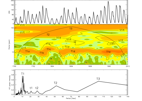
Fig. 1 : The long periodic modes of solar activity derived from the annual averaged relative sunspot number (ASN) during 1700 - 2011. The upper panel is the profile of ASN, the middle panel is the power spectrogram of Morlet wavelet analysis, and the lower panel is the corresponding Fourier power spectra of the Fast Fourier transformation.

Fig. 2 : The comparison of the profile (upper panels) and Fourier power spectra of the Fast Fourier Transformation (lower panels) between the solar microwave emission flux at frequency of 2.80 GHz and the daily relative sunspot number (RSN) from 1965-01-01 to 2011-12-31.

The estimation of frequency errors of FFT analysis can be obtained by the Nyquist theorem: $\frac{1}{2L}$, where $L$ is the length of time series of the data. The period obtained from the peak value of FFT spectrum symbolized as $P_{0}$, the corresponding frequency is $f_{0}=1/P_{0}$, then the frequency range is $f_{0}\pm 1/(2L)$. The period range is from $1/(f_{0}+\frac{1}{2L})$ to $1/(f_{0}-\frac{1}{2L})$, approximately,

$$P\approx P_{0}\pm\frac{P_{0}^{2}}{2L}.$$ (1)

(2) Wavelet Transformation

The second method is wavelet transform analysis, which is a powerful tool for analyzing localized power variations in a time series data set, and can give the scale and time position of a periodic phenomenon occurred. Here we use the Morlet wavelet transformation (MWT) to determine the possible periodic modes concealed in the long-term observation data of ASN, RSN, and $F_{28}$. MWT is defined as a complex sine wave localized in a Gaussian window (Morlet et al. 1982). The result of MWT can be plotted as a spectrogram in time-period space, where an obvious period mode is represented by a bright strip, the brighter the strip, the higher the confidence level. From the time-period spectrum, we may find out when the periodic mode occurred, and how the period changes with time.

The middle panel of Figure 1 is the power spectrogram of MWT on ASN during 1700-2011, which presents the detailed information of solar long-term periodic modes.

Generally, the main features of solar activity are extremely different from the peak years to the vale years in solar Schwabe cycles. The daily $F_{28}$ and RSN covers more than 4 solar Schwabe cycles and 17166 d, the whole power spectrum of MWT indicates that the periodic modes around the peak years of the solar cycles are different from that around the vale years of the solar cycles. So, when we investigate the solar mid-term periodic modes we divide the 5-day averaged data set of each solar cycle into peak years and vale years. The peak years of cycle 20-23 are 1966-1972, 1978-1984, 1988-1994, and 1999-2005; the vale years of cycle 20-23 are 1972-1978, 1984-1988, 1994-1999, and 2005-2011. Then we make MWT analysis on each data paragraph, respectively. Figure 3 and Figure 4 are the MWT power spectrograms on the 5-day averaged F28 and the 5-day averaged RSN around peak years and vale years in solar Schwabe cycle 20-23, respectively, which may present the detailed information of solar mid-term periodic modes.

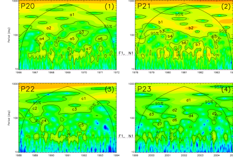
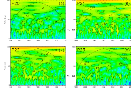
Fig. 3 : The comparison of the power spectrogram of MWT analysis between the 5-day averaged F28 and the 5-day averaged RSN around the peak years in solar Schwabe cycle 20-23.

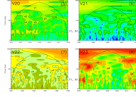
Fig. 4 : The comparison of the power spectrograms of MWT analysis between the 5-day averaged F28 and the 5-day averaged RSN around the vale years in solar Schwabe cycle 20-23.

In each panel, we find that there is an identical periodic mode marked by the horizontal dotted line, and the corresponding period is about 27 d. This mode is just the one derived from the above FFT power spectra (F1 and N1). Obviously, it is most possibly generated from the solar rotation. We do not discuss it in this work.

3 Main Results of the Solar Periodic Modes

3.1 The Long-term Periodicity

The first glance at the profile of ASN in the upper panel of Figure 1 may tell us that there are at least two distinct different periods: one has a timescale of about 11 yr (in the range of 9.5-13.5 yr), the other has a timescale of about 103 yr. The former is the well-known solar Schwabe cycle. The later is always called as solar secular cycle (Gleissberg, 1939, etc.).

The Fourier power spectra of FFT analysis in the lower panel of Figure 1 indicates that there are at least several periodic components: three periods with the confidence level of 95%: 11 yr (marked as T1), $52\pm 4.3$ yr (T2, 47.7-56.3 yr), and $103\pm 17$ yr (T3, 86-120 yr); two periods with the confidence level of 90%: $21.5\pm 0.74$ yr (t1, 20.76-22.24 yr) and $28.5\pm 1.3$ yr (t2, 27.2-29.8 yr). Here, the errors are obtained from Equation (1). In fact, from a scrutinizing of the FFT spectrum, we may find that the famous Schwabe Cycle (T1) is a mixture of 3 different components: $10\pm 0.16$ yr, $11.1\pm 0.20$ yr, and $11.9\pm 0.23$ yr. t1 is always regarded as the solar magnetic cycle with 22 yr period.

The power spectrogram of MWT analysis on ASN in the middle panel of Figure 1 shows that the Schwabe cycle is a bright band around 11 yr with the band width of 9.5-13.5 yr (T1a-T1e); T2 is relative weak in the range of 50-55 yr; and T3 is a strong periodic component in the range of 90-110 yr; t1 (t1a and t1b) and t2 also falls into the 95% confidence level on the power spectrum of MWT. The similar results can also be seen in previous works, for example, the co-existence of about 11-yr, 52-yr and 103-yr in Le and Wang (2003), Tan (2011). Otaola and Zenteno (1983) reported the evidence of 21.5-yr and 28.5-yr solar cycles.

3.2 The Mid-term Periodicity

From the investigation of 5-day averaged $F_{28}$ and RSN from 1965-01-01 to 2011-12-31, we obtain the details of the mid-term periodicity of solar activity. At first, the FFT power spectra of 5-day averaged $F_{28}$ shows the following mid-term periodic modes: $900\pm 23.6$ d (marked as F2), $53\pm 0.08$ d (f1), $75\pm 0.16$ d (f2), $115\pm 0.39$ d (f3), $145\pm 0.61$ d (f4), $280\pm 2.3$ d, $230\pm 1.5$ d, $330\pm 3.2$ d and $400\pm 4.7$ d (f5 and its adjacent), and $680\pm 13.5$ d (f6) (left panels of Figure 2). The FFT power spectra of 5-day averaged RSN can show the evidence of mid-term periodic modes with confidence level $>95\%$: $690\pm 13.9$ d (N2), $54\pm 0.16$ d (n1), $90\pm 0.24$ d, $105\pm 0.32$ d, and $116\pm 0.39$ d (n2 and its adjacent), $140\pm 0.57$ d (n3), $235\pm 1.6$ d (n4), $395\pm 4.5$ d (n5) (right panels of Figure 2).

The panels (1), (2), (3), and (4) of Figure 3 are the MWT power spectrum of 5-day averaged F28 around the peak years of solar cycle 20-23, respectively. Several mid-term periodic modes are noted. In cycle 20 (panel 1): 360 d (a1), 145 d (a2), 115 d (a3), 85 d (a4 and a5); in cycle 21 (panel 2): 235 d (b1), 148 d (b2), 120 d (b3), 90 d (b4 and b5), 54 d (b6), 50 d (b7); in cycle 22 (panel 3): 370 d (c1), 200 d (c2); 180 d (c3), 88 d (c4), and 60 d (c5); in cycle 23 (panel 4): 320 d (d1), 150 d (d2), 118 d (d3 and d5), 115 d (d4), 88 d (d6); and 60 d (d7).

The panels (5), (6), (7), and (8) of Figure 3 are the MWT power spectrum of 5-day averaged RSN around the peak years of solar cycle 20-23, respectively. Several mid-term periodic modes can be noted. In cycle 20 (panel 5): 370 d (k1), 145 d (k2), 116 d (k3); 80 d (k4, k5, and k6); in cycle 21 (panel 6): 360 d (m1), 150 d (m2), 120 d (m3 and m5), 54 d (m4, m6, and m7); in cycle 22 (panel 7): 400 d (y1), 190 d (y2), 180 d (y3), 85 d (y4), 70 d (y5), 83 d (y6), and 54 d (y7); in cycle 23 (panel 8): 310 d (p1), 120 d (p2 and p4), 90 d (p3), and 83 d (p5).

The panels (1), (2), (3), and (4) of Figure 4 are the MWT power spectrogram of 5-day averaged F28 around the vale years of solar cycle 20-23, respectively. The mid-term periodic modes are as following. In cycle 20 (panel 1): 400 d (e1), 118 d (e2), 115 d (e3), 80 d (e4 and e6); 86 d (e5), and 60 d (e7); in cycle 21 (panel 2): 300 d (g1), 88 d (g2), and 90 d (g3); in cycle 22 (panel 3): 120 d (h1 and h2), 54 d (h3 and h4); in cycle 23 (panel 4): 240 d (q1), 190 d (q2), 118 d (q3), 100 d (q4), 85 d (q5) and 80 d (q6).

The panels (5), (6), (7), and (8) of Figure 4 are the MWT power spectrogram of 5-day averaged RSN around the vale years of solar cycle 20-23, respectively. Several mid-term periodic modes can be noted: in cycle 20 (panel 5): 400 d (s1), 147 d (s2), 116 d (s3), 85 d (s4), and 86 d (s5); in cycle 21 (panel 6): 180 d (x1), 90 d (x2 and x3), 54 d (x2 and x3); in cycle 22 (panel 7): 120 d (u1), 85 d (u2), 54 d (u3), 73 d (u4); in cycle 23 (panel 8), 240 d (v1), 210 d (v2), 118 d (v3), 100 d (v4), and, 54 d (v5).

In brief, the main mid-term periodic modes of solar activity can be listed as following:

P1: 53-54 d, occurred in Figure 2 (f1 and n1), Figure 3 (b6 and m4), Figure 4 (h3, h4, x4, x5, and v5), the averaged value is about 53 d.

P2: 85-90 d, occurred in Figure 2 (n2 adjacent), Figure 3 (a4, a5, b4, b5, c4, d4, y4, and p3), and Figure 4 (e5, g2, g3, q5, s4, s5, x2, x3, and u2), the averaged value is about 89 d.

P3: 115-120 d, occurred in Figure 2 (f3 and n2 adjacent), Figure 3 (a3, b3, d3, d5, d4, k3, m3, m4, p2 and p4), and Figure 4 (e2, e3, h1, h2, q3, s3, u1, and v3), the averaged value is about 117 d.

P4: 140-150 d, occurred in Figure 2 (f4 and n3), Figure 3 (a2, b2, d2, k2, and m2), and Figure 4 (s2), the averaged value is 146 d.

P5: 230-240 d, occurred in Figure 2 (f5 adjacent, n4), Figure 3 (b1), and Figure 4 (q1 and v1), the averaged value is about 236 d.

P6: 360-370 d, occurred in Figure 3 (a1, c1, and k1), the averaged value is about 367 d.

P7: 395-400 d, occurred in Figure 2 (f5 adjacent and n5), Figure 3 (y1), and Figure 4 (e1 and s1), the averaged value is about 399 d.

Here, we neglect other periodic modes which are also occurred but not frequently in the above analysis, such as 60 d, 75 d, 200 d, 320 d, etc. In the previous literatures, several similar mid-term periodic modes of solar activity are also reported. Kilcik et al. (2010) show the existence of 53 d, 85 d, 115 d, 137 d, 152 d, and 248 d periodic modes derived from solar flare index. Pap, Tobiska, and Bouwer (1990) gave the evidence of 113 d and 237 d periodic modes. Caballero & Valdes-Galicia (2003) reported the 89 d and 115 d periodic modes from the records in a high altitude neutron monitor. The famous Rieger period with 138-159 d is frequently reported from publications (Rieger, et al. 1984, etc.).

3.3 Comparison between the solar cycles and the planetary motions

It is well known that the most obvious periodic modes in solar system are the planetary motions around the Sun. These periodic motions include planetary sidereal motions around the Sun producing tidal forces and the conjunction motions of two or more planets producing spring tidal forces on solar mass, and the latter can be called as spring tidal period. The spring tidal period of two planets can be calculated by: $P=\frac{1}{2}\frac{P1\cdot P2}{P1-P2}$, and its integral multiples are also spring tidal periods. Here $P1$ and $P2$ are the sidereal periods of the two planets, respectively. For example, we may obtain the spring tidal period of Mercury and Jupiter at 89.77 d, and 115.89 d for Mercury and Earth, 144.55 d for Mercury and Venus, 236.97 d for Venus and Jupiter, 398.88 d for Earth and Jupiter, etc. It has been found that Venus, Earth and Jupiter tend to be mostly aligned every 11.07 yr (Takahashi, 1968; Scafetta, 2012a, etc.). With these periodic motions, the planetary gravitational forces acting on solar mass will undergo periodic variations. It is questionable whether these periodic variations of the planetary forces can trigger the periodic solar activity or not. However, it is also meaningful to make a comprehensive comparison between the solar periodic modes and the planetary motions.

Here, we define a parameter $\beta$ to measure the similarity between the solar activity periodic modes and the corresponding planetary periods:

$$\beta=\frac{|P_{sa}-P_{sp}|}{P_{sp}}.$$ (2)

Here $P_{sa}$ is the period of solar activity, and $P_{sp}$ is the period of planetary sidereal motions or the conjunction motion of two or more planets. We find that there are 9 periodic modes of solar activity to be very close to some planetary sidereal periods or spring tidal periods of two or more planets. We may name such kind of periodic modes as planetary-like cycles (PLC), and symbolize them as:

PLC1: P2 (85-90 d, averaged value 89 d) is close to the spring tidal period of Mercury and Jupiter (89.77 d), the averaged $\beta\approx 0.87\%$. The Mercury sidereal period (88.0 d) is also very close to P2, and the value of $\beta$ is about 1.13%.

PLC2: P3 (115-120 d, averaged value 117 d) is close to the spring tidal period of Mercury and Earth (115.89 d), the averaged $\beta\approx 0.95\%$.

PLC3: P4 (140-150 d, averaged value 146 d) is close to the spring tidal period of the Mercury and Venus (144.55 d), the averaged $\beta\approx 0.99\%$.

PLC4: P5 (230-240 d, averaged value 236 d) is close to the spring tidal period of Venus and Jupiter (236.97 d), the averaged $\beta\approx 0.41\%$.

PLC5: P6 (360-370 d, averaged value 367 d) is close to the sidereal period of Earth (365.25 d), $\beta\approx 0.48\%$.

PLC6: P7 ($\sim$400 d) is close to the spring tidal period of Earth and Jupiter (398.88 d), the averaged $\beta\approx 0.28\%$.

PLC7: the overall effect of T1 (9.5-13 yr with the averaged value 11.2 yr) is the most prominent Schwabe 11-yr cycle which is always regarded as having some links with the Jupiter’s motion. In fact, PLC7 is actually a mixture of 3 different components: PLC7-1: $10\pm 0.16$ yr (9.84-10.16), very close to a half of the spring tidal period of Jupiter and Saturn (9.93 yr). The averaged values of $\beta$ is 0.70%; PLC7-2: $11.1\pm 0.20$ yr (10.90-11.30), very close to period of the conjunction motion of Venus, Earth and Jupiter (11.07 yr). The averaged values of $\beta$ is 0.27%; and PLC7-3: $11.9\pm 0.23$ yr (11.67-12.13), very close to Jupiter sidereal period (11.86 yr). The averaged values of $\beta$ is 0.31%.

PLC8: t1 ($21.5\pm 0.74$ yr) is close to the synodic period of Jupiter and Saturn (19.87 yr), and the averaged value of $\beta$ is 8.2%. There is an another possibility that the 21.5-yr periodic mode is a resonance mode of 2 times of the 11.07-yr conjunction motion period of Venus, Earth and Jupiter (Scafetta, 2012b). In such regime, $\beta\sim 3\%$. Furthermore, as the error range also beyond 3%, so far, we have no enough evidences to determine which one is true.

PLC9: t2 ($28.5\pm 1.3$ yr) is close to the sidereal period of Saturn (29.42 yr), the difference is from -2.22 yr to 0.38 yr, and the averaged value of $\beta$ is 3.1%.

The above results indicate that there are only a few not many periodic modes of solar activities seemed to have no relationship with the planetary motions. Most of the periodic modes of solar activities are PLCs, possibly associated to the planetary motions. According to the values of $\beta$, we may classify these PLCs into two kinds:

(1) Strong PLC, which has relatively short period ($P<12$ yr), low $\beta$ value, $\beta<1.0\%$, and related to the motions of the inner planets and the Jupiter, including PLC1, PLC2, PLC3, PLC4, PLC5, PLC6, and PLC7 (at the same time, PLC7 contains 3 different periodic modes).

(2) weak PLC, which has relatively long period ($P>12$ yr), high $\beta$ value, $\beta>3.0\%$, and possibly related to the motions of outer planets, including PLC8 and PLC9. At the same time, we also notice that the intrinsic error exceeds 3% when the period beyond 20 yr. Therefore, $\beta<1.0\%$ is only a moderate parameter when we determine which mode belongs to weak PLC.

There are also several periodic modes which seems no obvious relationship with planetary motions. We may call them as Non-PLC. This class includes the modes with period of 53-54 d, 70-75 d, $52\pm 4.3$ yr (T2, 47.7-56.3 yr), and $103\pm 17$ yr (T3, 86-120 yr).

4 Physical Discussions

The relatively close equality of the averaged solar Schwabe cycle period and the sidereal period of Jupiter was noticed for a long time. Since the 19th century a theory has been proposed claiming that the solar activity is partially driven by the planetary tidal forces (Wolf, 1859; Jose, 1965; Wood, 1975; Landscheidt 1999). However, most existing literature focuses on discussing the relationship between the solar Schwabe cycle with period of about 11 yr and the orbital motion of Jupiter. The physics of the periodic modes of solar activity with multiple timescales is still an open question. We need to answer the following questions: how strong the planetary gravitational force acting on the solar plasmas? what kind of planetary motion dominate which solar periodic mode? what is the physical mechanism of the PLC?

Many people believe that $F_{td}$ acting on the solar mass may result in the solar activity (Jose 1965, Landscheidt 1999, Scafetta 2012). As the tachocline layer is most possibly the source region of the solar magnetic fields (Parfrey and Menou 2007, etc.), similar to the other authors, we also calculate $F_{td}$ at tachocline layer:

$$F_{td}=\frac{2GM_{p}R_{t}}{a_{p}^{3}}=\frac{GM_{p}}{a_{p}^{2}}\frac{2R_{t}}{a_{p}}$$ (3)

Here, $M_{p}$ is the planet mass, $R_{t}$ is the solar radius at tachocline level, $a_{p}$ is the averaged distance between the Sun and the planet. Here we define a force unit $sgu$ as 1% gravitational force acting on unit solar mass operated by Earth, 1$sgu=1.782\times 10^{-10}m\cdot s^{-2}$. During the spring tides, $F_{td}$ is the sum of the tidal forces of the corresponding planets. Table 1 lists a series of tidal forces, including several spring tidal forces.

Furthermore, Equation (3) indicates that the tidal force is proportional to the radius. The solar photospheric mass will suffer a stronger tidal force than that of the solar internal mass. Even if the solar magnetic field possibly originates at the tachocline level, solar eruptions (solar flares, CME, and eruptive filaments, etc.) take place in the solar atmosphere, especially in the solar chromosphere and corona.

Table 1 : Planetary tidal forces (unit in $sgu$), listed by the decreasing order. $P_{td}$ is the corresponding period. Here abbreviations of Mc, V, E, Mr, J, S, U, and Np express Mercury, Venus, Earth, Mars, Jupiter, Saturn, Uranus, and Neptune, respectively. The unit of $\phi$ is $sgu/yr$.

planet	$F_{td}$	$P_{td}$	$\phi$	$P_{sa}$	$\beta(\%)$
V/E/J	3.53	11.07yr	0.637	11.1yr	0.27
V/J	2.88	236.9d	8.865	236d	0.41
E/J	2.12	398.9d	3.888	400d	0.28
Mc/J	2.09	89.8d	17.02	89d	0.87
Mc/V	2.03	144.6d	10.23	146d	0.99
J/S	1.54	9.93yr	0.310	10.0yr	0.70
J/S	1.54	19.87yr	0.156	21.5yr	8.20
J	1.47	11.86yr	0.248	11.9yr	0.31
V	1.40	224.7d	4.564	–	–
Mc/E	1.27	115.9d	8.023	117d	0.95
E	0.65	365.2d	1.304	367d	0.48
Mc	0.62	88.0d	5.155	–	–
S	0.07	29.42yr	0.004	28.5yr	3.13
Mr	0.02	686.9d	0.021
U	$<$0.01	83.75yr	$<$0.001
Np	$<$0.01	163.7yr	$<$0.001

De Jager and Versteegh (2005) compared the three accelerations working on the solar matter at the tachocline level: the acceleration due to $F_{td}$, the one due to the motion of the sun around the mass center of the solar system with the sum of planetary attractions, and the actual one due to connective motions in the tachocline level and above it. Supposed an averaged solar convective velocity at the bottom of the convection zone, then the actual acceleration near the tachocline level is about $6\times 10^{-6}m\cdot s^{-2}\simeq$ $3.36\times 10^{4}$ sgu (Robinson et al. 2004). They found that the later is much larger than the former two by several orders of magnitude, and pointed out that the planetary attraction is not the cause of solar activity, the main cause is purely originated from the solar interior. Callebaut, de Jager and Duhau (2012) reconsidered the internal convective velocity, examined the magnetic buoyancy and Coriolis force, and deduced that the planetary influences are too weak to be even a small modulation of the solar cycles.

However, as we know that solar atmosphere is a huge plasma system, any equilibrium in such system is always flimsy and most unstable, even with a very small perturbation, the system will lost its equilibrium, and a variety of instabilities are very easy to develop, accumulate, and trigger a considerable outburst. Recently, Shravan, Thomas, and Katepalli (2012) use techniques of helioseismology to image the flows in solar interior, and find that the solar convective velocities are 20-100 times weaker than the previous theoretical estimations. If this fact is true, it will reduce the gap between the solar interior convective velocity and the planetary tidal motions to some extent.

In order to investigate the change rate of planetary tidal force acting on solar mass operated by the planets during each PLC, we define another parameter, $\phi$, it can be calculated by:

$$\phi=\frac{F_{td}}{(1/2)P_{sp}}.$$ (4)

Here, $F_{td}$ is the planetary tidal force or the spring tidal force of conjunction motions of two or more planets, the unit of $\phi$ is sgu/yr. The $\phi$ values are listed in the fourth column of Table 1. As a comparison, the periods and $\beta$ are also listed in fifth and sixth column.

We find that the tidal force of conjunction motion of Venus, Earth and Jupiter is the strongest one (3.53 sgu) with period of 11.07 yr, which is related to the solar periodic mode of 11.1 yr, this mode is just the one closest to the central period of the most famous Schwabe Cycle. Table 1 shows that most tidal forces associated with PLCs have the value $F_{td}>1.0$ sgu. The sidereal tidal force of Venus is 1.40 sgu, but its period (224.7 d) is very close to the spring tidal period of Venus and Jupiter ($F_{td}=2.88$ sgu) and easy to be submerged in the latter.

By adopting the parameter $\phi$, we find that all the strong PLCs have the values $\phi>0.2$ sgu/yr, and $\phi<0.2$ sgu/yr for all weak PLCs. In this regime, we find that the biggest $\phi$ value is related to the conjunction motion of the Mercury and Jupiter (17.02 sgu/yr), the second biggest $\phi$ value is related to the conjunction motion of Mercury and Venus (10.23 sgu/yr). The $\phi$ values of the sidereal motions of Mercury is very big, however, because the Mercury sidereal period is very close to the spring tidal period of Mercury and Jupiter, which is very easy to be submerged in the latter. The Venus’s condition is similar to the Mercury’s.

Table 1 indicates that tidal forces operated by Mars, Uranus, and Neptune are very weak relative to the other 5 planets by several orders of magnitudes, that we may neglect their tidal effects on solar activities. Jupiter plays a key role in most periodic modes by its own sidereal motion or conjunction motion with other planets (PLC1, PLC4, PLC5, PLC7-1, PLC7-2, PLC7-3, and PLC8). Additionally, some of inner planets, such as Mercury, Venus and Earth also play important roles in the formation of PLCs.

The conjunction motion and the related spring tidal forces of the planets dominate the formation of most PLCs. Such as the conjunction motion of Venus/Earth/Jupiter, Venus/Jupiter, Earth/Jupiter, Mercury/Jupiter, Mercury/Venus, Mercury/Earth, and Jupiter/saturn. This is understandable, because the strongest tidal force acted by any individual planet is only 1.47 sgu (Jupiter), while many spring tidal forces acted by conjunction motion of two or more planets are stronger than that acted by Jupiter alone. As mentioned above, the conjunction motion of Venus, Earth and Jupiter forms the strongest periodic mode of 11.07 yr and related to the most famous Schwabe cycle.

Fig. 5 : The relationships between period (P) and the change rate of planetary tidal force acting on solar mass operated by the planets (Phi). Triangle represents the strong PLC, and plus sign represents the weak PLC.

Figure 5 shows the relationships between period ($P$) and $\phi$. It indicates that PLCs have an obvious tendency of the value $\phi$ decreasing with the period increasing. Particularly, strong PLCs (triangle signs) are much more obvious with such tendency, while the weak PLCs (plus signs) are more disperse.

Some people will also suspect that $F_{td}$ is still too weak to excite a considerable perturbation in solar atmosphere. And the difference between the planetary periods and the periods of PLC also let us to distrust the relationships between planetary motion and the solar periodical activity. As we know that solar atmosphere is a huge magnetized plasma system, any equilibrium in such system is flimsy and most unstable. Even if a very small perturbation can also disrupt the magnetized plasma system, make it lost the equilibrium, and trigger a considerable instability. Such instability can accumulate in a complicated way, and result in energy releasing. Finally, the solar activity bursts out. The enormous energy released in the solar activity is essentially originated from the solar inner processes. Here, $F_{td}$ just plays a role of blasting fuse of solar activity. Recently, Scafetta (2012b) proposed that the planetary tidal gravitational energy can amplify the nuclear fusion in the solar core region, and result in the solar periodic activities. Maybe this is a possible physical mechanism. Based on the tidal cycles of the Jupiter and Saturn plus the dynamo theory, Scafetta (2012a) has shown that it is possible to reconstruct solar variability with a high accuracy at the decadal, secular and millennial timescale throughout the Holocene.

5 Conclusions

This work presents a comprehensive investigations of the quasi-periodic modes of solar activity with multi-timescale and their relationships with the planetary periodic motions. From this investigation, we may get the following conclusions:

(1) All the periodic modes of solar activities can be classified into 3 classes:

A. Strong PLC, which is related strongly with planetary motions. This class includes 8 periodic modes: PLC1 (85-90 d, averaged period is 89 d, close to the spring tidal period of Mercury and Jupiter), PLC2 (115-120 d, averaged period is 117 d, close to the spring tidal period of Mercury and Earth), PLC3 (140-150 d, averaged period is 146 d, close to the spring tidal period of Mercury and Venus), PLC4 (230-240 d, averaged period is 236 d, close to the spring tidal period of Venus and Jupiter), PLC5 (400 d, close to the spring tidal period of Earth and Jupiter), PLC6 (360-370 d, close to the sidereal period of Earth), PLC7-1 (10 yr, close to the spring tidal period of Jupiter and Saturn), PLC7-2 (11.1 yr, close to the spring tidal period of Venus, Earth and Jupiter), PLC7-3 (11.9 yr, close to the sidereal period of Jupiter). This class mode has relatively short period ($P<12$ yr), $\phi>0.2$ sgu/yr, low $\beta$ value, $\beta<1.0\%$, and related to the motions of the inner planets and of Jupiter.

B. Weak PLC, which is related weakly with planetary motions. This class includes 2 periodic modes: PLC8 (21.5 yr, close to the synodic period of Jupiter and Saturn) and PLC9 (28.5 yr, close to the sidereal period of Saturn). This class mode has relatively long period ($P>12$ yr), $\phi<0.2$ sgu/yr, high $\beta$ value, $\beta>3.0\%$, and possibly related to the motions of outer planets. At the same time, because periods of weak PLCs are always very long, and their error levels are always very large, the uncertainty of weak PLCs can not be neglected.

C. Non-PLC, which is so far regarded as no obvious relationship with any planetary motions. This class includes the modes with period of 53-54 d, 70-75 d, $52\pm 4.3$ yr (T2, 47.7-56.3 yr), and $103\pm 17$ yr (T3, 86-120 yr).

(2) Among all the planets, Jupiter plays a key role in most periodic modes by its own sidereal motion or conjunction motion with other planets. 7 PLCs (PLC1, PLC4, PLC5, PLC7-1, PLC7-2, PLC7-3, and PLC8) are dominated by Jupiter.

(3) Among all the planetary motions, the conjunction motion of the inner planets dominated the formation of most PLCs. Such as the conjunction motion of Venus/Earth/Jupiter, Venus/Jupiter, Earth/Jupiter, Mercury/Jupiter, Mercury/Venus, Mercury/Earth, and Jupiter/saturn, etc.

The closely connection between the mid-term periodic modes of solar activity and the planetary motions may imply that it can be applied to predict the solar activity in the near future. In our next step researches, we will focus on investigating the effects of the planetary motions to the solar short- and mid-term activity, and the detailed processes of the physical mechanism.

Acknowledgements

The authors would like to thank the referee’s valuable comments on the manuscript and SGD teams for the systematic data. This work is supported by MOST Grant No. 2011CB811401, NSFC Grant No. 11273030, 10921303, and the National Major Scientific Equipment R&D Project ZDYZ2009-3.

References

- Caballero (2003) Caballero, R., & Valdes-Galicia, J.F.: 2003, Solar Phys. 213, 413.
- Callebaut (2012) Callebaut, D.K., de Jager, C., & Huhau, S.: 2012, J. Atmospher. Sol. Terr. Phys., 80, 73
- de Jager (2005) de Jager, C., & Versteegh, G.J.M.: 2005, Solar Phys. 229, 175.
- Frick et al (1997) Frick, P., Galyagin, D., Hoyt, D.V., et al.: 1997, Astron Astrophys 328, 670.
- Gleissberg (1939) Gleissberg, W.: 1939, Observatory 62, 158.
- Gleissberg (1971) Gleissberg, W.: 1971, Solar Phys. 21, 240.
- Hiremath (2009) Hiremath, K.M.: 2009, arXiv0909.4420[astro-ph.SR].
- Jose (1965) Jose, P.D., 1965, AJ, 70, 193
- Kilcik (2010) Kilcik, A., Ozguc, A., Rozelot, J.P., & Atas, T. 2010, Solar Phys., 264, 255.
- Kundu (1960) Kundu, M.R., 1960, J. Grophys. Res., 65, 3903.
- Landscheidt (1999) Landscheidt, Th, 1999, Solar Phys., 189, 415.
- Le (2003) Le, G.M., & Wang, J.L.: 2003, Chin. J. Astron. Astrophys., 3, 391.
- Morlet (1982) Morlet, J., Arehs, G., Forgeau, I., Giard, D.: 1982, Geophysics, 47, 203.
- Nagovitsyn (1997) Nagovitsyn, Yu A.: 1997, Astron Lett 23, 742.
- Otaola & Zenteno (1983) Otaola, J.A.Q., & Zenteno, G.: 1983, Solar Phys. 89, 209.
- Parfrey (2007) Parfrey, K.P., & Menou, K.: 2007, ApJ, 667, L207.
- Pap (1990) Pap, J., Tobiska, W.K., & Bouwer, S.D.: 1990, Solar Phys., 129, 165.
- Rieger (1984) Rieger, E., Kanbach, G., Reppin, C., Share, G.H., Forrest, D.J., & Chupp, E.L.: 1984, Nature 312, 623.
- Robinson (2004) Robinson, F.J., Demarque, P, Li, L.A., Sofia, S., Kim, Y.-C., Chan, K.L., Guenther, D.B.: 2004, Mon. Not. R. Astron. Soc., 340, 923.
- Scafetta1 (2012a) Scafetta, N.: 2012a, J. Atmospher. Sol. Terr. Phys., 80, 296.
- Scafetta2 (2012b) Scafetta, N.: 2012b, J. Atmospher. Sol. Terr. Phys., 81-82, 27.
- Schove (1979) Schove, D.J.: 1979, Solar Phys. 63, 423.
- Shravan (2012) Shravan, M.H., Thomas, L.D., Jr., Katepalli, R.S.: 2012, PNAS 109, 11928.
- Suess (1980) Suess, H.E.: 1980, Radiocarbon 20, 200.
- Takahashi (1968) Takahashi, K.: 1968, Solar Phys., 3, 598.
- Tan (2011) Tan, B.L. 2011, ApSS, 332, 65.
- Yoshimura (1978) Yoshimura, H. 1978, ApJ, 226, 706.
- Wolf (1859) Wolf, R.: 1859, Mon. Not. R. Astron. Soc., 19, 85.
- Wolff (2010) Wolff, C.L., & Patrone, P.N.: 2010, Solar Phys., 266, 227.
- Wood (1975) Wood, R.M.: 1975, Nature 255, 312.