Radio-frequency magnetometry using a single electron spin

Abstract

We experimentally demonstrate a simple and robust protocol for the detection of weak radio-frequency magnetic fields using a single electron spin in diamond. Our method relies on spin locking, where the Rabi frequency of the spin is adjusted to match the MHz signal frequency. In a proof-of-principle experiment we detect a $7.5\,\mathrm{MHz}$ magnetic probe field of $\sim 40\,\mathrm{nT}$ amplitude with $<10\,\mathrm{kHz}$ spectral resolution. Rotating-frame magnetometry may provide a direct and sensitive route to high-resolution spectroscopy of nanoscale nuclear spin signals.

Quantum systems have been recognized as extraordinarily sensitive detectors for weak magnetic and electric fields. Spin states in atomic vapors budker07 or flux states in superconducting quantum interference devices ryhanen89 , for example, offer among the best sensitivities in magnetic field detection. Trapped ions maiwald09 or semiconductor quantum dots vamivakas11 are investigated as ultrasensitive detectors for local electric fields. The tiny volume of single quantum systems, often at the level of atoms, furthermore offers interesting opportunities for ultrasensitive microscopies with nanometer spatial resolution degen08 ; gierling11 ; grinolds12 .

Sensitive detection of weak external fields by a quantum two-level system is most commonly achieved by phase detection: In Ramsey interferometry, a quantum system is prepared in a superposition $\frac{1}{\sqrt{2}}\left(|0\rangle+|1\rangle\right)$ of states $|0\rangle$ and $|1\rangle$, and then left to freely evolve during time $\tau$. During evolution, state $|1\rangle$ will gain a phase advance $\Delta\phi=\tau\Delta E/\hbar$ over $|0\rangle$ (where $\Delta E$ is the energy separation between $|0\rangle$ and $|1\rangle$) that is manifest as a coherent oscillation between $\frac{1}{\sqrt{2}}\left(|0\rangle\pm|1\rangle\right)$ states. These oscillations can be detected either directly or by back-projection onto $|0\rangle$ and $|1\rangle$. For spin systems, which are considered here, the energy splitting sensitively depends on magnetic field $B$ through the Zeeman effect $\Delta E=\hbar\gamma B$ (where $\gamma$ is the gyromagnetic ratio), allowing very small changes in $B$ to be measured for spins with long coherence times $\tau$.

In its most basic variety, phase detection measures DC or low frequency ($\sim\,\mathrm{kHz}$) AC fields that fluctuate slower than $\tau$; in other words, the free evolution process effectively acts as a low-pass filter with bandwidth $\propto\tau^{-1}$. Spin echo and multi-pulse decoupling sequences have been introduced to shift the detection window to higher frequencies while maintaining the narrow filter profile kotler11 ; delange11 . Going to higher frequencies is advantageous for two reasons: Firstly, coherence times generally increase, allowing for longer evolution times and better sensitivities. Additionally, spectral selectivity can be drastically improved. While multi-pulse decoupling sequences work well for capturing $\lessapprox 1\,\mathrm{MHz}$ signals delange11 , extending this range to the tens or hundreds of MHz – an attractive frequency range for nuclear spin detection – is impractical due to the many fast pulses required for spin manipulation. Moreover, the response function of multi-pulse sequences has multiple spectral windows that complicate interpretation of complex signals.

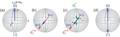
Figure 1: Illustration of rotating frame magnetometry using the Bloch sphere: (a) An electron spin is initialized into the $|0\rangle$ state and transferred into the coherent superposition $|x+\rangle=\frac{1}{\sqrt{2}}(|0\rangle+e^{i\omega_{0}t}|1\rangle)$. (b) A microwave field $B_{1}^{\mathrm{mw}}e^{i\omega_{0}t}$ is applied in-phase with the spin precessing around the $z$ axis. (c) During sensing period $\tau$, transitions are induced between $|x+\rangle$ and $|x-\rangle=\frac{1}{\sqrt{2}}(|0\rangle-e^{i\omega_{0}t}|1\rangle)$ states by weak radio-frequency fields $B^{\mathrm{rf}}e^{i\Omega t}$ if the rf frequency $\Omega$ matches the Rabi frequency $\omega_{1}=\gamma B_{1}^{\mathrm{mw}}$. (d) $|x+\rangle$ ($|x-\rangle$) states are transferred to detectable $|0\rangle$ ($|1\rangle$) polarization. The transition probability $|x+\rangle\leftrightarrow|x-\rangle$ is equal to the probability of measuring $|1\rangle$.

Presented here is a simple and robust method to directly detect $\gg 1\,\mathrm{MHz}$ magnetic signals with high sensitivity and spectral selectivity. Our approach relies on spin locking slichter ; cai11 ; hirose12 and is illustrated in Fig. 1: In a spin-lock experiment, a resonant microwave field is applied in-phase with the coherent Larmor precession of the spin. In the picture of a reference frame rotating at the Larmor frequency $\omega_{0}=\Delta E/\hbar$ (rotating frame), the microwave field appears as a constant field parallel to the spin’s orientation. In this frame of reference, the spin is quantized along the microwave field axis with an energy separation of $\hbar\omega_{1}=\hbar\gamma B_{1}^{\mathrm{mw}}$ between states parallel and anti-parallel to the microwave field, where $B_{1}^{\mathrm{mw}}$ is the amplitude ($\omega_{1}$ the Rabi frequency) of the microwave field. If now an additional, weak rf magnetic field whose frequency $\Omega$ matches the Rabi frequency is present, transitions between parallel and anti-parallel states are induced at a rate set by the magnitude $B_{1}^{\mathrm{rf}}$ of the rf field redfield55 . Since Rabi frequencies can be precisely tuned over a wide MHz frequency range by adjusting microwave power fuchs09 , the single electron spin can act as a wide range, narrow band, and sensitive detector for rf magnetic fields.

Symbol	Range	Description
$\omega_{0}$	GHz	Spin Larmor frequency
$\omega$	GHz	Microwave frequency
$B_{1}^{\mathrm{mw}}$	$\mu$T-mT	Microwave amplitude
$\omega_{1}=\gamma B_{1}^{\mathrm{mw}}$	MHz	Microwave amplitude (in units
		of frequency); Spin Rabi frequency
$\Omega$	MHz	RF frequency
$B_{1}^{\mathrm{rf}}$	nT-$\mu$T	RF amplitude
$\Omega_{1}=\gamma B_{1}^{\mathrm{rf}}$	kHz	RF amplitude (in units of frequency)

Table 1: List of symbols.

In the following we consider in general terms the transition probability $p$ between $|x+\rangle$ and $|x-\rangle$ states (see Fig. 1) in response to a coherent and to a stochastic rf magnetic probe field. This situation is equivalent to the classical problem of a two-level system interacting with a radiation field rabi37 ; wang45 ; cummings62 . For the case of a coherent driving field $B_{1}^{\mathrm{rf}}e^{i\Omega t}$ oriented along the $z$-axis (see Fig. 1), the transition probability $p$ is given by cummings62 ; rabi37 ,

$$p=p_{0}\frac{\Omega_{1}^{2}}{\Omega_{1}^{2}+(\Omega-\omega_{1})^{2}}\sin^{2}\left(\sqrt{\Omega_{1}^{2}+(\Omega-\omega_{1})^{2}}\frac{\tau}{2}\right),$$ (1)

where $p_{0}\leq 1$ is the maximum achievable transition probability, $\Omega_{1}=\gamma B_{1}^{\mathrm{rf}}$ is the amplitude of the rf field, and other symbols are collected in Table 1. (If a detuning $\omega-\omega_{0}$ were present, $\omega_{1}$ would need to be replaced by the effective Rabi frequency $\omega_{\mathrm{eff}}=\sqrt{\omega_{1}^{2}+(\omega-\omega_{0})^{2}}$.) We notice that $B_{1}^{\mathrm{rf}}$ will drive coherent oscillations between states, and that the spectral region that will respond to $B_{1}^{\mathrm{rf}}$ is confined to either $\omega_{1}\pm\Omega_{1}$ or $\omega_{1}\pm 5.57/\tau$, whichever is larger supplementary . This corresponds to a detector bandwidth set by either power or interrogation time.

Alternatively, for stochastic magnetic signals, the transition probability can be analyzed in terms of the magnetic noise spectral density $S_{B}(\omega)$ cummings62 ; wang45 ,

$$p=\frac{p_{0}}{2}\left(1-e^{-\tau/T_{1\rho}}\right)$$ (2)

where $T_{1\rho}$ is the rotating frame relaxation time slichter ,

$$T_{1\rho}^{-1}=\frac{1}{4}\gamma^{2}\left[S_{B_{z}}(\omega_{1})+S_{B_{y}}(\omega_{0})\right],$$ (3)

and $S_{B_{z}}(\omega_{1})$ and $S_{B_{y}}(\omega_{0})$ are the magnetic noise spectral densities evaluated at the Rabi and Larmor frequencies, respectively, and $z$ and $y$ are given according to Fig. 1. Thus, measurements of $T_{1\rho}$ for different $\omega_{1}$ can be used to map out the spectral density bylander11 ; bargill12 . Eq. (2) only applies for uncorrelated magnetic noise (correlation time $\tau_{c}<\tau$). A more general expression that extends Eq. (3) to an arbitrary spectral density is discussed in Ref. cummings62 .

Eqs. (1-3) describe the general response of an ideal two-level system in the absence of relaxation and inhomogeneous line broadening. Regarding relaxation we note that the contrast $p_{0}$ will be reduced to $p_{0}e^{-\tau/T_{1\rho}}$ for long evolution times $\tau\gtrsim T_{1\rho}$, where $T_{1\rho}$ is the rotating frame relaxation time due to magnetic fluctuations in the sensors’ environment [Eqs. (2,3)]. Thus, relaxation imposes a limit on the maximum useful $\tau$, which in turn limits both sensitivity (see below) and minimum achievable detection bandwidth.

Line broadening of the electron spin resonance (ESR) transition can be accounted for by a modified transition probability $\tilde{p}$ that is averaged over the ESR spectrum $q(\omega_{0})$ cummings62 ,

$$\tilde{p}=\int_{0}^{\infty}d\omega_{0}q(\omega_{0})p(\omega_{0}),$$ (4)

where $q(\omega_{0})$ is normalized to unity. $p(\omega_{0})$ is given by Eq. (1) and depends on $\omega_{0}$ through the effective Rabi frequency $\omega_{\mathrm{eff}}=\sqrt{\omega_{1}^{2}+(\omega-\omega_{0})^{2}}$. As an example, if $q(\omega_{0})$ is a Gaussian spectrum with a linewidth sigma $\sigma_{\omega_{0}}$ and center frequency detuned by $\Delta\omega_{0}=\omega-\omega_{0}$ from the microwave frequency $\omega$, the associated linewidth of the rotating-frame spectrum is

$$\sigma_{\omega_{1}}\approx\sigma_{\omega_{0}}\left[\frac{\Delta\omega_{0}^{2}}{\omega_{1}^{2}}+\frac{\sigma_{\omega_{0}}^{2}}{4\omega_{1}^{2}}\right]^{1/2}.$$ (5)

Inhomogeneous broadening of the ESR spectrum therefore leads to an associated inhomogeneous broadening of the rotating-frame spectrum that is scaled by $\frac{\sigma_{\omega_{0}}}{2\omega_{1}}$ or $\frac{\Delta\omega_{0}}{\omega_{1}}$, respectively. Since $\omega_{1}\gg\sigma_{\omega_{0}},\Delta\omega_{0}$, narrow linewidths can be expected even in the presence of a significant ESR linewidth.

Finally, we can estimate the sensitivity towards detection of small magnetic fields. For small field amplitudes $\Omega_{1}<\tau^{-1}$ the transition probability [Eq. (1)] reduces to $p\approx p_{0}\frac{1}{4}\Omega_{1}^{2}\tau^{2}$. Assuming that the transition probability is measured with an uncertainty of $\sigma_{p}$ (due to detector noise), we obtain a signal-to-noise ratio (SNR) of $\mathrm{SNR}=\frac{p}{\sigma_{p}}=\frac{p_{0}}{4\sigma_{p}}\Omega_{1}^{2}\tau^{2}$. The corresponding minimum detectable field $B_{\mathrm{min}}=\Omega_{1}/\gamma$ (for unit SNR) is

$$B_{\mathrm{min}}=\frac{2}{\gamma\tau}\sqrt{\frac{\sigma_{p}}{p_{0}}}.$$ (6)

Eq. (6) outlines the general strategy for maximizing sensitivity: $\tau$ should be made as long as possible, $\sigma_{p}$ should be reduced (by optimizing read-out efficiency), and $p_{0}$ should be made as large as possible (by keeping $\tau<T_{1\rho}$ and avoiding inhomogeneous broadening) supplementary .

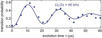
Figure 2: Coherent oscillation between $|x+\rangle$ and $|x-\rangle$ states induced by a rf probe field of $B_{1}^{\mathrm{rf}}=1.6\,\mathrm{\mu T}$. Solid line is a fit to a decaying sinusoid supplementary . $\Omega$ and $\omega_{1}$ are both $2\pi\cdot 7.5\,\mathrm{MHz}$. Symbols are explained in Table 1.

We demonstrate rotating-frame magnetometry by detecting weak (nT-$\mu\mathrm{T}$) rf magnetic fields using a single nitrogen-vacancy defect (NV center) in an electronic-grade single crystal of diamond oforiokai12 . The NV center is a prototype single spin system that can be optically initialized and read-out at room temperature jelezko06 and that has successfully been implemented in high-resolution magnetometry devices balasubramanian08 ; rondin12 ; grinolds12 . Following Fig. 1, we initialize the NV spin ($S=1$) into the $|0\rangle$ ($m_{S}=0$) state by optical pumping with a $\sim 1\,\mu{\rm s}$ green laser pulse, and transfer it into spin coherence $|x+\rangle$ (where $|1\rangle$ corresponds to $m_{S}=+1$) using an adiabatic half-passage microwave pulse slichter . The spin is then held under spin-lock during $\tau$ by a microwave field of adjustable amplitude. After time $\tau$, the state is transferred back to $|0\rangle$ (or $|1\rangle$) polarization, and read out by a second laser pulse using spin-dependent luminescence jelezko06 . The final level of fluorescence (minus an offset) is then directly proportional to the probability $p$ of a transition having occurred between $|x+\rangle$ and $|x-\rangle$. Precise details on experimental setup and microwave pulse protocol are given as Supplemental Material supplementary .

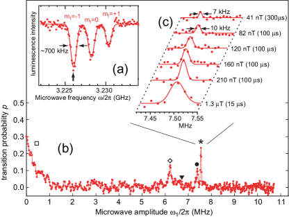
Figure 3: (a) Optically-detected electron spin resonance (ESR) spectrum of one of the NV centers used for experiments. Dots are data, solid lines are Gaussian fits. $m_{I}=\pm 1$, $m_{I}=0$ indicate hyperfine lines ($a=2.2\,\mathrm{MHz}$) associated with the ¹⁴NV nuclear spin ($I=1$). Microwave frequency used in spin-lock experiments was always centered on the $m_{I}=-1$ line, indicated by an arrow. DC bias field was $17\,\mathrm{mT}$. (b) Rotating-frame spectrum with 7.5 MHz probe field present (feature $\star$). Other features are explained with Fig. 4. Evolution time was $\tau=15\,\mathrm{\,\mu{\rm s}}$. (c) High-resolution spectra of the main peak ($\star$) for longer evolution times and weaker probe fields. Dots are data, solid lines are Gaussian fits. Linewidths are full width at half maximum. Numbers indicate $B_{1}^{\mathrm{rf}}$ and $\tau$. Baseline noise of the 41-nT spectrum corresponds to 8 nT ($\sigma_{p}=0.020$), and an integration time of 840 s per point was used.

In a first experiment, shown in Fig. 2, we demonstrate the driving of coherent oscillations between parallel and anti-parallel states. For this purpose, the microwave amplitude was adjusted to produce a Rabi frequency of $7.5\,\mathrm{MHz}$, and a small rf probe field of the same frequency was superimposed. The transition probability $p$ was then plotted for a series of interrogation times $\tau$. The period of oscillations allows for a precise calibration of the rf magnetic field, which in this case was $B_{1}^{\mathrm{rf}}=\Omega_{1}/\gamma=1.65\,\mathrm{\mu\mathrm{T}}$. While one would expect $p$ to oscillate between 0 and 1, this probability is reduced because we mainly excite one out of the three hyperfine lines of the NV center (see below). The decay of oscillations is due to inhomogeneous broadening of the ESR linewidth and a slight offset $\Omega-\omega_{\mathrm{rf}}$ between RF and Rabi frequencies supplementary .

Fig. 3 presents a spectrum of the transition probability up to microwave amplitudes $\omega_{1}/2\pi$ of $11\,\mathrm{MHz}$ with the same rf probe field present. A sharp peak in transition probability is seen at 7.5 MHz (marked by $\star$), demonstrating that the electron spin indeed acts as a spectrally very selective rf magnetic field detector. Inset (c) plots the same 7.5 MHz peak for longer evolution times and weaker probe fields, revealing that for long $\tau$, fields as small as about $40\,\mathrm{nT}$ ($1.1\,\mathrm{kHz}$) can be detected and linewidths less than $10\,\mathrm{kHz}$ (0.13%) are achieved. For comparison, the detection bandwidth [$2\times 5.57/\tau$, see Eq. (1)] is $3.2\,\mathrm{kHz}$ for the 41-nT-spectrum and $8.8\,\mathrm{kHz}$ for the 82-nT-spectrum, in reasonable agreement with the experiment. The $\sim 700\,\mathrm{kHz}$ linewidth of the ESR transition [Fig. 3(a)] translates into an inhomogeneous broadening of about $18\,\mathrm{kHz}$ [Eq. (5)], which is somewhat higher than the experiment (since the ESR linewidth is likely overestimated). The narrow spectra together with little drift in line position furthermore underline that power stability in microwave generation (a potential concern with spin-locking) is not an issue here.

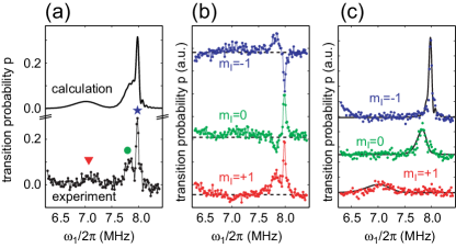
Figure 4: (a) Rotating-frame spectrum showing the three peaks associated with $m_{I}=-1(\star)$, $m_{I}=0(\bullet)$, and $m_{I}=1(\blacktriangledown)$. Solid line is a calculation based on Eq. (4) and the EPR spectrum shown in Fig. 3(a). Parameters are identical to Fig. 3 except for $\Omega/2\pi=8\,\mathrm{MHz}$. (b) Spectra as-recorded using spin state selection. (c) Linear recombination of pure-state spectra from data in (b). Solid line is the calculated response.

Several additional features can be seen in the spectrum of Fig. 3. The increase in $p$ below $1\,\mathrm{MHz}$ (marked by $\square$) can be attributed to nearby ¹³C diamond lattice nuclear spins ($I=\frac{1}{2}$, 1% natural abundance) with hyperfine couplings in the 100’s of kHz range, causing both spectral broadening and low frequency noise. The feature ($\diamond$) appearing at $\sim 6\,\mathrm{MHz}$ is of unknown origin; since it is absent for NV centers composed of the ¹⁵N nuclear isotope it is probably related to the nuclear quadrupole interaction of ¹⁴N supplementary . The peak at $\sim 7.3\,\mathrm{MHz}$ ($\bullet$) finally is a replica of the main $7.5\,\mathrm{MHz}$ peak ($\star$) associated with the $m_{I}=0$ nuclear ¹⁴NV spin sublevel: Since the microwave field excites all three hyperfine lines [see Fig. 3(a)], the rotating-frame spectrum is the stochastic thermal mixture of three different Larmor transitions with different effective Rabi frequencies. Only two out of three peaks are visible in Fig. 3; all three peaks can be seen in a higher resolution spectrum shown in Fig. 4(a). This presence of hyperfine lines is undesired, as it can lead to spectral overlap and generally complicates interpretation of the spectrum.

In Fig. 4 we show how this complexity can be removed using spin state selection duma03 . For this purpose, we invert the electronic spin conditional on the ¹⁴N nuclear spin state before proceeding with the spin-lock sequence. Conditional inversion is achieved by a selective adiabatic passage over one hyperfine line. In the spectrum this leads to selective inversion of peaks associated with that particular nuclear spin state. Fig. 4(b) shows the resulting spectra for all three sublevels. By linear combination of the three spectra (or by subtraction from the non-selective spectrum) we can then reconstruct separate, pure-state spectra for each $m_{I}$ sublevel. Fig. 4(c) shows that spin state selection is very effective in removing the hyperfine structure in the spectrum. We note that other schemes could also be used, such as initialization of the nuclear spin by optical pumping jacques09 or more general spin bath narrowing strategies cappellaro12 .

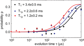
Figure 5: Relaxation time measurements for bulk (black squares and blue circles) and shallow implanted (5 nm deep, red triangles) NV centers show approximately $T_{1}$-limited behavior.

Finally, we have determined the baseline magnetic noise spectral density $S_{B}(\omega)$ for two representative NV centers using relaxation time measurements. Fig. 5 plots $T_{1}$ and $T_{1\rho}$ decay curves for a bulk and a shallow-implanted ($\sim 5\,\mathrm{nm}$) NV center oforiokai12 . From the $T_{1}$ measurement we infer $S_{B}^{1/2}(\omega_{0})=\sqrt{2/(\gamma^{2}T_{1})}\approx 0.14\,\mathrm{nT/\sqrt{\mathrm{Hz}}}$ (per magnetic field orientation), evaluated at $\omega_{0}/2\pi=3.2\,\mathrm{GHz}$. From $T_{1\rho}$ measurements we obtain $S_{B}^{1/2}(\omega_{1})\approx 0.20-0.30\,\mathrm{nT/\sqrt{\mathrm{Hz}}}$, evaluated at $\omega_{1}/2\pi=7\,\mathrm{MHz}$. Thus, for these experiments we conclude that $S_{B}^{1/2}(\omega_{1})$ is similar, if slightly higher than $S_{B}^{1/2}(\omega_{0})$, and measurements are approximately $T_{1}$-limited. Since $T_{1}$ itself is likely limited by thermal phonons and could be enhanced to $<1\,\mathrm{pT/\sqrt{\mathrm{Hz}}}$ by going to cryogenic temperatures jarmola12 , there is scope for further improvement at lower temperatures.

In conclusion, we have demonstrated how a single electronic spin can be harnessed for radio-frequency magnetic field detection with high sensitivity and excellent spectral resolution. Our protocol relies on spin-locking and is found to be robust and simple, requiring a minimum of three microwave pulses. Although the radio-frequency range addressed in our demonstration experiment was limited to roughly $0-11\,\mathrm{MHz}$ by efficiency of microwave delivery, it is easily extended to several hundred MHz using more sophisticated circuitry, such as on-chip microstrips fuchs09 .

We anticipate that rotating-frame magnetometry will be particularly useful for the detection and spectral analysis of high-frequency signals in nanostructures, such as in small ensembles of nuclear and electronic spins. For example, the magnetic stray field of a single proton spin at 5 nm distance is on the order of 20 nT degen08 . These specifications are within reach of the presented method and engineered shallow diamond defects oforiokai12 ; ohno12 , suggesting that single nuclear spin detection could be feasible. In contrast to other nanoscale magnetic resonance detection methods, such as magnetic resonance force microscopy poggio10 single electron spin sensors are ideally suited for high-resolution spectroscopy applications because they operate without a magnetic field gradient.

The authors gratefully acknowledge financial support through the NCCR QSIT, a competence center funded by the Swiss NSF, and through SNF grant $200021\_137520/1$. We thank K. Chang, J. Cremer, R. Schirhagl, and T. Schoch for the help in instrument setup, sample preparation and complementary numerical simulations. C. L. D. acknowledges support through the DARPA QuASAR program.

References

- (1) D. Budker, and M. Romalis, Nat. Phys. 3, 227 (2007).
- (2) T. Ryhanen, H. Seppa, R. Ilmoniemi, and J. Knuutila, J. Low Temp. Phys. 76, 287-386 (1989).
- (3) R. Maiwald et al., Nature Physics 5, 551 (2009).
- (4) A. N. Vamivakas et al., Phys. Rev. Lett. 107, 166802 (2011).
- (5) C. L. Degen, Appl. Phys. Lett. 92, 243111 (2008).
- (6) M. Gierling et al., Nat. Nanotechnol. 6, 446-451 (2011).
- (7) M. S. Grinolds et al., arXiv:1209.0203 (2012).
- (8) G. De Lange, D. Riste, V. V. Dobrovitski, and R. Hanson, Phys. Rev. Lett. 106, 080802 (2011).
- (9) S. Kotler, N. Akerman, Y. Glickman, A. Keselman, and R. Ozeri, Nature 473, 61-65 (2011).
- (10) C. P. Slichter, Principles of Magnetic Resonance, (Springer, Heidelberg, 1996).
- (11) J.-M. Cai, F. Jelezko, M. B. Plenio, A. Retzker, arXiv:1112.5502 (2011).
- (12) M. Hirose, C. D. Aiello, and P. Cappellaro, arXiv:1207.5729 (2012).
- (13) A. G. Redfield, 98, 1787-1809 (1955).
- (14) G. D. Fuchs, V. V. Dobrovitski, D. M. Toyli, F. J. Heremans, and D. D. Awschalom, Science 326, 1520-1522 (2009).
- (15) F. W. Cummings, Am. J. Phys. 30, 898 (1962).
- (16) I. I. Rabi, Phys. Rev. 51, 0652-0654 (1937).
- (17) M. C. Wang, and G. E. Uhlenbeck, Rev. Mod. Phys. 17, 323 (1945).
- (18) See Supplemental Material accompanying this manuscript.
- (19) J. Bylander et al., Nat. Phys. 7, 565-570 (2011).
- (20) N. Bar-Gill et al., Nat. Commun. 3, 858 (2012).
- (21) B. K. Ofori-Okai et al., Phys. Rev. B 86, 081406 (2012).
- (22) F. Jelezko, and J. Wrachtrup, phys. stat. sol. (a) 203, 3207 (2006).
- (23) G. Balasubramanian et al., Nature 455, 648 (2008).
- (24) L. Rondin et al., Appl. Phys. Lett. 100, 153118 (2012).
- (25) L. Duma, S. Hediger, A. Lesage, and L. Emsley, J. Magn. Reson. 164, 187-195 (2003).
- (26) V. Jacques et al., Phys. Rev. Lett. 102, 057403 (2009).
- (27) P. Cappellaro, Phys. Rev. A 85, 030301 (2012).
- (28) A. Jarmola, V. M. Acosta, K. Jensen, S. Chemerisov, and D. Budker, Phys. Rev. Lett. 108, 197601 (2012).
- (29) K. Ohno et al., Appl. Phys. Lett. 101, 082413 (2012).
- (30) M. Poggio, and C. L. Degen, Nanotechnology 21, 342001 (2010).