Classical Light Sources with Tunable Temporal Coherence and Tailored Photon Number Distributions

Abstract

We demonstrate a method for the generation of tunable classical light sources with electronic control over its temporal characteristics and photon number distribution by modulating coherent light. The tunability of the temporal coherence is shown through second order correlation ($G^{2}(\tau)$) measurements both in the continuous intensity measurement as well as in the photon counting regimes. The generation of desired classical photon number distributions is illustrated by creating two light sources - one emitting thermal state and the other a specific classical non-Gaussian state. Such tailored light sources with emission characteristics quite different from that of existing natural light sources are likely to be useful in quantum information processing for example in conjunction with photon addition to possibily generate tailored non-clasical states of light. As a particular application in this direction we outline how a classical non-Gaussian state generated in this manner may be mixed with an appropriate non-classical Gaussian state at a beamsplitter, to generate non-Gaussian entanglement.

I introduction

Understanding light-matter interactions and mechanisms of light generation are of vital importance in elucidating many physical processes. While for most processes, a combination of a statistical approach along with Maxwell’s classical theory of electromagnetism suffices, several optical processes demand a quantum mechanical approach to the electromagnetic field Glauber ; sudarshan63 ; Fermi-Quantum . The quantum theory of light makes a clear distinction between different sources of radiation such as coherent, thermal, and single photon sources Glauber-Coherent . Radiation from the former two sources may be explained classically, while light from the latter can only be explained quantum mechanically. In other words, the former two states are deemed classical, and the latter non-classical. Due to their quantum nature, non-classical sources of light display several counter-intuitive features evoking considerable interest in them. Non-classical sources of light have been generated experimentally by several techniques single-photon and their possible applications in different fields, especially quantum information, are well explored Review . However, recent years have witnessed an emergence of interest in classical sources of light SHIH-THERMAL-IMAGING -alessia These have been used in intriguing applications like ghost imaging SHIH-THERMAL-IMAGING -lugiato06 , and interferometry based experiments as in Refs. sam-french ; nandan-sam , and have also formed an ingredient in the creation of non-classical states of light zavatta07 ; parigi09 ; keisel11 .

In this paper we demonstrate a method of creating classical incoherent light sources that can be tailored to mimic light from a thermal source or can be made to emit light quite distinct from that emitted by natural light sources. Utilizing the fact that an acousto-optic modulator (AOM) may be effectively used to introduce phase and intensity fluctuations to light rapidly and accurately Elliot ; Nandan ; quantumwalk , we create incoherent light having the desired coherence times and intensity statistics, or photon-number distributions, from input coherent light. The motivations for creating such sources are several. This technique offers an alternative to the current standard method of using a rotating ground glass plate Martien ; arecchi65 to generate pseudo-thermal light. Further, the electronic control of fluctuations provides a robust and flexible procedure for producing tailored classical light sources with predetermined photon emission rates. Several interesting applications now become possible. For example, it is known that non-classical states can be generated by combining classical light, both coherent and thermal, with single photons (Fock state) in photon addition experiments zavatta07 -keisel11 ,gsa -Grangier-Science . The ability to tailor classical states of light to have Gaussian or non-Gaussian photon number distributions as demonstrated in this paper, widens the field of generation of non-classical states of light by making many novel forms possible. In addition, classical non-Gaussian states with tailored photon number distributions (PND) may, in turn, be used to produce states with tailored non-Gaussian entanglement. This is of importance in the quantum information theoretic context, where recent findings suggest non-Gaussian entanglement to be advantageous over Gaussian entanglement solop ; dellanno07 ; dellano08 .

This paper is arranged as follows. The experimental setup used in this study is described in Section $2$. Section 3 describes the methodology for the generation of classical incoherent light with tunable temporal coherence. This is achieved by imparting random phase shifts to coherent light through the acousto-optic interaction, in a Mach-Zehnder interferometer (MZI). Measurements of the second-order correlation function, $G^{2}(\tau)$, both using a classical photodetector (intensity-intensity correlation) and photon counting detector (photon coincidence detection), show the tunability of temporal characteristics, and the equivalence of the two forms of detection. In Section 4, we generate classical light sources with the desired PNDs introducing intensity fluctuations to light by suitably modulating the diffraction efficiency of the acousto-optic modulator (AOM). Two incoherent states, one thermal and the other a classical non-Gaussian state were created as illustrative examples. In Section $5$ we discuss the possible use of such tailored classical non-Gaussian state in producing tailored non-classical states and non-Gaussian entanglement. Section $6$ summarizes the work presented in this paper.

II Experimental Setup

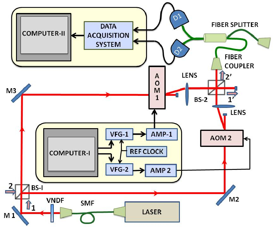
Figure 1: Schematic of the experiment. AMP - amplifier, AOM - acousto-optic modulator, BS - beam splitter, D1,D2 - detectors, M1 - M3 - mirrors, SMF - single mode fiber, VFG - versatile function generator, VNDF - variable neutral density filter.

The schematic of the experiment is given in Fig. 1. Coherent cw laser light from an external cavity diode laser (Toptica, 767 nm, linewidth $<5$ MHz) was fiber coupled through a single mode polarization maintaining fiber. The light was then passed through a variable neutral density filter (VNDF) ( to control the intensity of the beam) onto beam splitter BS1 where it was amplitude divided into two parts. These two beams traversed along the two arms of a Mach-Zehnder interferometer (MZI), which had an AOM in each of the two arms, arranged such that the first order diffracted light proceeded further on, while the undiffracted light was blocked. After traversing the two arms of the interferometer, the beams were combined at BS2, that is, the diffracted light beams of the two arms of the MZI interfered at BS2. Light emerging from one of the exit ports of BS2 was directed into an input of a 50:50 fiber-splitter, and then onto two detectors, D1 and D2.

The two AOMs were driven by individual Versatile Function Generators (VFG, Toptica) which operated at 80 MHz radio frequency (rf); they were both referenced to a common 10MHz clock. Using a LabVIEW interface we could tailor any distribution of phase and intensity fluctuations in the rf electrical signal being fed to the AOM on time scales ranging from few hundreds of nanoseconds to seconds. These fluctuations were transferred to the diffracted light by the acousto-optic interaction thus providing fine electronic control over the phase and intensity of the light. Measurements at the two detectors were used to determine the second order correlation (intensity-intensity correlation) function. For the case of continuous light intensity measurements, the laser was operated at a power of around $30\,\rm mW$ and D1 and D2 were two fast photodiodes (Thorlabs PD10A-EC). For the case of photon coincidence detection, the laser light was strongly attenuated, photodiodes D1 and D2 were avalanche photo-diode (APD) based single photon counting modules ( SPCM-AQR-15 Perkin Elmer) where an incident photon results in a TTL pulse with a detection efficiency of 65 % at 767 nm spcm . The outputs of D1 and D2 were stored in a PC using data acquisition systems. In the case of classical detectors, a digital storage oscilloscope was employed, while for photon counting, two counters on a data acquisition card (NI M-series PCI-6259) were used.

III Generation of Incoherent Light by only phase modulation in an MZI setup

In this Section, we describe the creation of incoherent sources of light by imparting phase jumps to light by means of the AOMs in the MZI (Fig.1). The use of a Mach-Zehnder interferometer was motivated by the facts that, i) phase changes imparted to light can be discerned only in an interferometric setup, and ii) it enables the creation of a source with intensity fluctuations even though only phase jumps are imparted to light.

III.1 Theory

The action of the MZI in Fig.1 may be mathematically represented by the transformation matrix $M=B.\Phi.B$ where $B$ ( the operation of a beam splitter) and $\Phi$ (the action of the two AOMs) are given by

$$B=\frac{1}{\sqrt{2}}\left(\begin{array}[]{cc}\,\,\,\,1&1\\ -1&1\end{array}\right)\,\,\,\,\rm and\,\,\,\,\,\,\Phi=\left(\begin{array}[]{cc}e^{i\phi_{1}(t)}&0\\ 0&e^{i\phi_{2}(t)}\end{array}\right)$$ (5)

Here $\phi_{1}(t)$ and $\phi_{2}(t)$ are the phase shifts imparted to light at AOMs 1 and 2, respectively. Thus, in terms of the scalar wave field, $E_{1}$, entering one of the ports of $BS1$ (and with no input at its other port) the output at $BS2$ is given by

$$\left(\begin{array}[]{c}E_{1^{\prime}}\\ E_{2^{\prime}}\end{array}\right) = M.\left(\begin{array}[]{c}E_{1}\\ 0\end{array}\right)$$ (10)

where 1, 2 represent the input ports of BS1 and 1’, 2’ the output ports of BS2. It is clear that the second order intensity self-correlation at the output ports is given by

$$G^{2}_{ii}(\tau)=\frac{\left\langle E_{i}^{\star}(t)E_{i}(t)E_{i}^{\star}(t+\tau)E_{i}(t+\tau)\right\rangle_{t}}{\left\langle E_{i}^{\star}(t)E_{i}(t)\right\rangle_{t}\left\langle E_{i}^{\star}(t+\tau)E_{i}(t+\tau)\right\rangle_{t}}$$ (11)

where i can take values 1’, 2’. In terms of field operators $G^{2}_{ii}(\tau)$ is given by

$$\frac{\left\langle\psi\right|A_{i}{}^{\dagger}(t)A_{i}{}^{\dagger}(t+\tau)A_{i}(t+\tau)A_{i}(t)\left|\psi\right\rangle_{t}}{\left\langle\psi\right|A_{i}{}^{\dagger}(t+\tau)A_{i}(t+\tau)\left|\psi\right\rangle_{t}\left\langle\psi\right|A_{i}{}^{\dagger}(t)A_{i}(t)\left|\psi\right\rangle_{t}}$$ (12)

where

$$\left(\begin{array}[]{c}\hat{A_{1^{\prime}}}\\ \hat{A_{2^{\prime}}}\end{array}\right)=M.\left(\begin{array}[]{c}\hat{a_{1}}\\ \hat{a_{2}}\end{array}\right),$$ (17)

with $\left|\psi\right\rangle$ being the input state, $\hat{a_{1}}$, $\hat{a_{2}}$ the annihilation operators of the input modes, and $\hat{A}_{1^{\prime}},\hat{A}_{2^{\prime}}$ those of the output modes, and $M$ is as defined earlier. In our setup, $\left|\psi\right\rangle=\left|E_{1}\right\rangle\otimes\left|0\right\rangle$, where $\left|E_{1}\right\rangle$ is a coherent state. Simplification of Eqs. 11 and 12, for the case of complete phase noise, (i.e., uniformly distributed noise, with phase spanning the entire circle) both yield

$$G^{2}_{ii}(\tau)=1+\left\langle\cos(\delta\phi(t))\cos(\delta\phi(t+\tau))\right\rangle_{t}$$ (18)

where $\delta\phi=\phi_{1}(t)-\phi_{2}(t)$. Note that we have adjusted the MZI to match the dynamical paths in both arms and, therefore, the phase difference is the difference in the phases imparted at the two AOMs.

The temporal coherence of light, emerging out of the port 2’, was determined by intensity correlation technique in a standard correlation setup developed by Hanbury-Brown and Twiss HBT . Equation (6) can be easily cast into the form

$$G^{2}_{2^{\prime}2^{\prime}}(\tau) = 1+0.5\xi(\tau),$$ (19)

where $\xi(\tau)$ represents the probability of temporal overlap of $\delta\phi(t)$ and $\delta\phi(t+\tau)$. In general, for complete phase noise given to AOM 1 and 2 and phase jumps occurring at time intervals $t$ given by independent distributions $P_{1}(t)$ and $P_{2}(t)$ respectively, we have

$$\xi(\tau)=\frac{\int_{\tau}^{\infty}(t-\tau)P_{1}(t)d(t)}{\int_{0}^{\infty}tP_{1}(t)d(t)}.\frac{\int_{\tau}^{\infty}(t-\tau)P_{2}(t)d(t)}{\int_{0}^{\infty}tP_{2}(t)d(t)}$$ (20)

For the special case where one of the phases, say $\phi_{2}(t)$, is held constant Eq. 20 reduces to

$$\xi(\tau)=\frac{\int_{\tau}^{\infty}(t-\tau)P_{1}(t)d(t)}{\int_{0}^{\infty}tP_{1}(t)d(t)}$$ (21)

III.2 Experimental Results

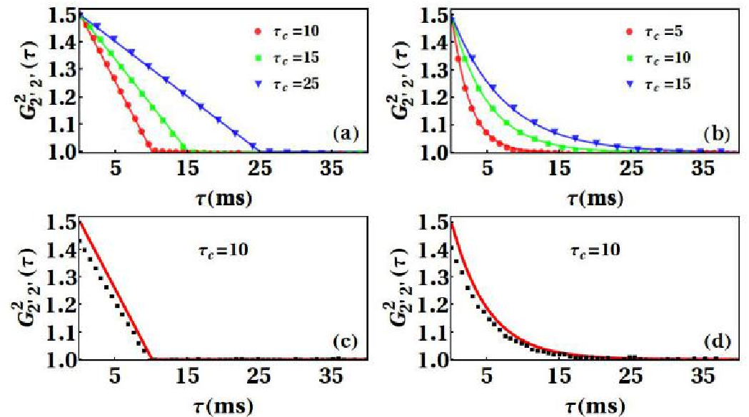
Figure 2: Intensity-intensity correlation function, $G^{2}_{2^{\prime}2^{\prime}}(\tau)$ of the light exiting port 2’ of BS2 in Fig.1, as function of $\tau$ for (a) constant dwell time noise to rf of one AOM, and with classical light detection; (b) exponential distribution of dwell times of noise in both AOMs, and with classical light detection; (c) same as (a), but in photon counting regime; (d) same as (b), but in photon counting regime.

We now present our experimental results. Initially, random phase jumps were imparted to AOM1 only and at regular intervals, that is, $P_{1}(t)=\delta(t-\tau_{c})$. For this case, we see from Eq. 21 and Eq. 19,

$$G^{2}_{2^{\prime}2^{\prime}}(\tau) = 1+0.5\left(1-\frac{\tau}{\tau_{c}}\right)\quad\rm for\quad\tau\leq\tau_{c}$$ (22)

$$= 1\quad\quad\quad\quad\quad\quad\quad\quad\rm for\quad\tau\geq\tau_{c}$$

that is, on imparting phase noise one expects photon-bunching with a zero-delay second-order correlation value 1.5, that falls to 1 for long delays. In the experiment, at constant time intervals, $\tau_{c}$, the rf electrical signal to AOM1 was given a random phase jump, distributed uniformly in the interval $(-\pi,\pi)$. The experimentally determined values of $G^{2}_{2^{\prime}2^{\prime}}(\tau)$ are shown as discrete points in Fig. 2(a) for three different values of coherence time, $\tau_{c}$. The continuous curves are $G^{2}_{2^{\prime}2^{\prime}}(\tau)$ as obtained from Eq. 22.

Next, AOMs 1 and 2 were driven with rf voltages with independent, random phase jumps uniformly distributed in the interval $(-\pi,\pi)$, and at time intervals that had independent exponentially falling distributions,  $P(t)=[\exp({-t/\tau_{c}})]/\tau_{c}$, with $1\,\rm ms$ $\leq t\leq 100\,\rm ms$ and with a mean, $\sim\tau_{c}.$ The results for this case are presented in Fig. 2(b), for three values of $\tau_{c}$. As in the previous case, the agreement between theory and experiment is very good.

The above measurements, which utilized classical detection of intensities with photodetectors, were repeated at the photon counting regime using APD based single-photon counting modules (SPCM). The laser light was strongly attenuated, so that, on an average, every $30\,\mu$s, there was a 10% probability of detecting a photon. Thus, there was, on an average, less than one photon in the interferometer at any instant of time. The output pulses from D1 and D2 (APD based SPCMs) were fed to two counters operating at a time bin of $30\,\mu$s, that was shorter than the mean interval between phase jumps that ranged from $1\,\rm ms$ to $100\,\rm ms$. The values of $G^{2}(\tau)$ obtained from the experiments for the two cases (phase jumps to one AOM only at constant intervals and phase jumps to both AOMs with exponential distribution of interval between jumps) are shown in Figs. 2(c) and 2(d), along with theoretically expected values. The agreement is fair. In order to obtain sufficient statistics at single photon detection level, data had to be acquired over long durations. Mechanical instability of the interferometer and dark counts are believed to have contributed to the deviation from the theoretical curves in the photon counting regime.

From the above, it is amply clear that classical light sources exhibiting bunching and with the desired temporal coherence characteristics may be created. The results also confirm the equivalence between classical intensity-intenstiy correlation and coincidence detection for $G^{2}(\tau)$ measurement for classical states of light. In the present experiment, the time scales for phase fluctuations are on the milliseconds time scales due to restriction of the data acquisition card. The setup allows for a temporal variation from  $50\,\rm ns$ (currently limited to $500\,\rm ns$ by USB 2.0 communication) to few seconds depending upon the stability of the interferometer. This provides an easy way of creating bunched light with long coherence times. Further the bunching can be enhanced and higher values of ${G^{2}_{2^{\prime}2^{\prime}}}(0)$ can be obtained by using engineered partial phase noise in this interferometric setup Nandan .

IV Tailoring Photon Number Distribution by Intensity Modulation of Light

In this Section, we demonstrate the creation of classical incoherent states with desired photon number distributions (PND), starting from an input coherent state. This was achieved by modulating the diffraction efficiency of a single AOM by the addition of calibrated amplitude noise with the desired characteristics to the input rf electrical signal. This, in effect, modulates the transmittivity of the coherent state through the AOM according to the chosen probability distribution function, thereby providing a source of classical light with a tailored photon number distribution.

IV.1 Theory

Consider the coherent state $|\alpha\rangle$ being diffracted by an AOM where the transmittivity into the diffracted order (amplitude of the coherent state) is modulated in time, in the from of ${\cal P}(|\alpha|)$. The modulated coherent state and its expansion in terms of number (Fock) states can be written as

$$\hat{\rho} = \int_{0}^{|\alpha_{0}|}{\cal P}(|\alpha|)|\alpha\rangle\langle\alpha|d^{2}|\alpha|=\sum_{n=0}^{\infty}p(n)|n\rangle\langle n|,\,\,\,\,{\rm with}$$

$$p(n) = \int_{0}^{|\alpha_{0}|}d^{2}|\alpha|\,{\cal P}(|\alpha|)\,e^{-|\alpha|^{2}}\,\frac{|\alpha|^{2n}}{n!}.$$ (23)

where $p(n)$ is the photon number distribution function and $|\alpha_{0}\rangle$ is the diffracted coherent state at maximal transmittivity, and $\{|n\rangle\}$ is the Fock basis. The ensemble in Eq. (23) is practically realized by appropriately modulating the transmittivity of the input coherent state over a sufficient amount of time. The upper limit of $\hat{\rho}$ can be taken as infinity if $|\alpha_{0}|$ is chosen to be much larger than the mean $|\alpha|$.

We experimentally generate light sources with two specific PNDs as examples. The first is the thermal state with an average of $\bar{n}$ photons, namely, $\hat{\rho}_{\rm th}(\bar{n})$  sudarshan63 with

$${\cal P}(|\alpha|)\equiv{\cal P}_{\rm th}(|\alpha|)=\frac{1}{\bar{n}\pi}\exp(-|\alpha|^{2}/{\bar{n}}),$$ (24)

for which the probabilities

$$p_{\rm th}(n)=({1-e^{-\lambda}})e^{-\lambda n}\,\,\,\,\,\,\,\rm with\,\,\,\,\,\,\,e^{-\lambda}=\bar{n}/(\bar{n}+1),$$ (25)

define the PND. The second is the state $\hat{\rho}_{\zeta}$ corresponding to

$${\cal P}(|\alpha|)\equiv{\cal P}_{\rm\zeta}(|\alpha|)=\zeta^{2}|\alpha|^{2}\exp[-\zeta|\alpha|^{2}],$$ (26)

with an average number of photons $\bar{n}$ and a PND specified by the probabilities

$$p_{\zeta}(n)=\left(\frac{\zeta}{\zeta+1}\right)^{2}\,\frac{n+1}{(\zeta+1)^{n}}.\,\,\,\,\,\,\,\rm with\,\,\,\,\,\,\,\zeta=\frac{2}{\bar{n}}.$$ (27)

Note that the state $\hat{\rho}_{\zeta}$ is manifestly non-Gaussian.

The temporal coherence characteristics of the incoherent light with tailored PNDs, as generated above, is described by the second-order correlation function $G^{2}(\tau)$, given by

$$G^{2}(\tau) = 1+(G^{2}(0)-1)\xi(\tau)$$ (28)

where $\xi(\tau)$ is as given in Eq. (21). $G^{2}(0)=2$ for ${\cal P}_{\rm th}(|\alpha|)$, $G^{2}(0)=1.5$ for ${\cal P}_{\zeta}(|\alpha|)$ and $G^{2}(0)=1$ for a coherent state.

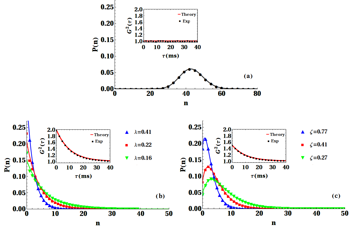
Figure 3: Photon number distributions, p(n) vs n, as determined from the experiment, with a time bin of 450$\mu$s, for (a) maximally diffracted laser light, in absence of input fluctuations; (b) light obtained with Gaussian amplitude noise (Eq. 12) applied to the rf, for different values of $\lambda$; (c) light obtained with non-Gaussian amplitude noise (Eq.14) applied to the rf, for different $\zeta$. Insets show the corresponding $G^{2}(\tau)$ as function of $\tau$.

IV.2 Experimental Results

For this part of the experiment AOM1 of Fig.1 was switched off and BS2 was removed. Thus, only the light emerging from AOM2 could reach the detectors, which in this case were APD based SPCMs, as described previously. The input laser beam was attenuated using neutral density filters to at most 94000 counts per second (cps), suitable for measurement in the photon counting regime spcm2 . The number distribution of photons was determined using a time bin of $450\,\mu$s. The size of the time bin, which determines the average photon number, was so chosen for the PND measurements to clearly bring out the distinction between coherent and incoherent states of various parameters. Once chosen this time bin was fixed for all PND determinations. All measurements lasted for a period of at least 30 minutes to obtain good statistics.

Initially, no noise was added to the rf signal and the maximum rf power was fed to the AOM; the $+1^{st}$ order diffracted light in this situation constitutes the maximally transmitted coherent state $|\alpha_{0}\rangle$. The PND for this light, as obtained from our measurements, is as shown in Fig. 3(a). It gave a Poissonian distribution with a mean photon number of 42 with an estimated average dark counts $2.25\times 10^{-2}$ spcm ; spcm2 per time bin, which is three orders of magnitude smaller than the average photon number in any of our experimental observations. The second-order correlation function, $G^{2}(\tau)$ for this case is shown in the inset; it is clearly that of a coherent state with $G^{2}(\tau)=1$ for all $\tau$. This was calculated directly from the recorded time series of the counter operating at $30\,\mu$s. Using the calibration of the AOM transmittivity into the $+1^{st}$ order versus the rf power, and the experimentally determined value of $\bar{n}$ for the maximally transmitted coherent state $|\alpha_{0}\rangle$, we generate, by appropriate modulation of rf power, light with the desired photon number distribution function. The rf power was fluctuated at random time intervals in the range $1$ to $100$ ms with a mean time of $\sim 10$ ms, with the distribution of time intervals falling exponentially.

Then the rf power fed to the AOM was varied such that the transmitted coherent state $|\alpha\rangle$ was modulated to realise ${\cal P}_{\rm th}(|\alpha|)$ of Eq.  $12$, for three different values of $\bar{n}$ ( 1.91, 3.85 and 5.67). The emergent light was found to have the PNDs as shown in Fig. 3(b). These are in good agreement with the theoretically expected curves given by Eq. 13 for ${p}_{\rm th}(n)$. The second-order correlation function for this case is shown in the inset. The zero-delay second-order correlation has a value 2, as expected for thermal light. This shows that temporal modulation of intensity of coherent light leads to the bunching of photons. On similar lines, the rf power fed to the AOM was varied such that the transmitted coherent state $|\alpha\rangle$ was modulated to realise the non-Gaussian function ${\cal P}_{\rm\zeta}(|\alpha|)$ of Eq.  $14$ for three different values of $\bar{n}$ (2.60, 4.88 and 7.41). The PNDs obtained for the emergent light are shown in Fig. 3(c), along with the theoretically expected curves given by Eq.  15 for ${p}_{\rm\zeta}(n)$ . The second order correlation function is shown in the inset. The zero-delay second-order correlation has a value 1.5, as expected for this case. The good agreement between theory and experiment for all measurements, both Gaussian and non-Gaussian, underlines the reliability and efficacy of this method in generating tailored classical light sources with desired PND and temporal coherence characteristics. Generation of classical non-Gaussian states with desired PND in a predetermined manner promises to be useful in various contexts as discussed in the next section.

V Application of classical non-Gaussian state in quantum optics

As our method offers complete flexibility of providing phase and/or intensity fluctuations with different desired probability distributions and on different time scales, the AOMs can be used to generate classical incoherent light having properties quite different from existing light sources, opening up new fields for exploration. For example it is a simple matter to produce light with temporal incoherence but spatial coherence. This is a crucial requirement in experiments involving photon addition/subtraction to incoherent lightparigi09 and this AOM-based technique is likely to find immediate application here. Another feature, likely to prove useful, is the ability to control the mean photon number with ease, even during the course of a measurement, by electronic means. This has been illustrated in Fig. 3(b) and 3(c), where we have changed the parameters $\lambda$ and $\xi$ to alter the mean photon number.

$\begin{array}[]{c c}\includegraphics[height=142.26378pt,width=204.85974pt]{P_th.jpg}&\includegraphics[height=142.26378pt,width=204.85974pt]{P_nongauss.jpg}\\ \end{array}$

Figure 4: The distribution function ${\cal P}(|\alpha|)$ for photon addded thermal state, $\rho^{1}_{th}$, (Fig.  (4) a)) and photon added classical non-Gaussian state, $\rho^{1}_{\zeta}$ (Fig.  (4) b)) given by Eq. 14. The plots for three different values of average photon number are given for each case. Note the qualitative difference between the two states for same average photon number.

V.1 Non-classical behaviour of photon added classical non-Gaussian state

A significant application of the tailored classical non-Gaussian states generated by this method is in the creation of tailored non-classical non-Gaussian states for example when used in conjunction with the photon addition technique. We consider the photon-added thermal state $\hat{\rho}_{\rm th}^{1}=\frac{1}{N_{1}}\,\hat{a}^{\dagger}\,\hat{\rho}_{\rm th}\,\hat{a}$ and the photon-added non-Gaussian state $\hat{\rho}_{\zeta}^{1}=\frac{1}{N_{2}}\,\hat{a}^{\dagger}\,\hat{\rho}_{\zeta}\,\hat{a}$. Here the superscript $1$ indicates that we have added one photon, and $N_{1}$ and $N_{2}$ are appropriate normalisations. The Glauber-Sudarshan’s diagonal weight functions sudarshan63 of the respective photon-added states are given by

$${\cal P}_{\rm th}^{1}(|\alpha|) = \frac{1}{\pi\,\bar{n}^{3}}\,(|\alpha|^{2}(1+\bar{n})-\bar{n})\,\exp[-|\alpha|^{2}/\bar{n}],\,$$

$${\cal P}_{\zeta}^{1}(|\alpha|) = \frac{4}{\pi\,\bar{n}^{4}\,(1+\bar{n})}\,(\bar{n}^{2}-3\bar{n}(\bar{n}+2)|\alpha|^{2}+(\bar{n}+2)^{2}|\alpha|^{4})\times$$ (29)

$$\exp[-2|\alpha|^{2}/\bar{n}],$$

with $\zeta=\frac{2}{\bar{n}}$ for the latter. As is well known, any state with a pointwise non-positive diagonal weight function is nonclassical (quantum). Clearly, both the weight functions in Eq. (29) correspond to nonclassical states, and this is made manifest in Figs. (4) a) and Figs. (4) b) . Further the nonclassicality (quantumness) of the states $\hat{\rho}_{\rm th}^{1}$ and $\hat{\rho}_{\zeta}^{1}$ are qualitatively different. To make this observation quantitative, we now evaluate the Mandel parameter $Q$, of these states with respect to the mean number of photons. The Mandel parameter $Q$ of a state $\hat{\rho}$ is defined as $Q=({\rm Tr}(\hat{\rho}\,\hat{a}^{\dagger 2}\hat{a}^{2})-({\rm Tr}(\hat{\rho}\,\hat{a}^{\dagger}\hat{a}))^{2})/{\rm Tr}(\hat{\rho}\,\hat{a}^{\dagger}\hat{a})$ mandel79 . As any state with $Q<0$ is definitely nonclassical (quantum), it is clear from Fig. (5) that both $\hat{\rho}_{\zeta}^{1}$ and $\hat{\rho}_{\rm th}^{1}$ show non-classical behaviuor. More interestingly, there are physical situations in which $Q$ of $\hat{\rho}_{\zeta}^{1}$ is $<0$ while $Q$ of $\hat{\rho}_{\rm th}^{1}$ $>0$ for the same mean no. of photons. This suggests tailoring the non-Gaussianity of a classical state can have a direct bearing on the quantum features that may emerge when such a state is subject to further quantum processing.

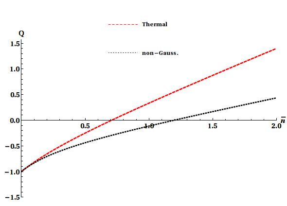
Figure 5: The differece in the non-classicality behaviour ($Q<0$) for the two different photon added states, one with thermal $\rho^{1}_{th}$ and other with non-Gaussain state $\rho^{1}_{\zeta}$. For the same mean photon number $\rho^{1}_{\zeta}$ shows more negativity compared to state $\rho^{1}_{th}$. Even more interestingly for mean photon numbers where $\rho^{1}_{th}$ is classical ($Q>0$), $\rho^{1}_{\zeta}$ still continues to be non-classical even upto average photon number $\bar{n}=1$.

V.2 Generation of non-Gaussian Entanglement

Here we show how the tailored PNDs of the kind generated above may be used for producing novel forms of entanglement.

As is well known, a beamsplitter preserves non-Gaussianity solo11-1 , and non-classicality sudarshan63 ; aharonov66 . It also generates entanglement of input non-classical states knight02 . These features of the beamsplitter may be utilized to create non-Gaussian entangled states [24] of the form

$$\hat{\rho}_{\rm out}^{\rm nG}=U_{bs}\,(\hat{\rho}_{\rm G}\otimes\hat{\rho}_{\rm nG})\,U_{bs}^{\dagger},$$ (30)

by appropriately choosing a Gaussian state $\hat{\rho}_{\rm G}$ and a tailored non-Gaussian state $\hat{\rho}_{\rm nG}$. Here $U_{bs}$ is the beamsplitter unitary.

Consider the situation where a single-mode squeezed state $\hat{\rho}_{\rm sq}$ enters one port of a 50:50 beamsplitter and a tailored non-Gaussian state $\hat{\rho}_{\rm nG}$ enters the other. Note that here we may also tailor the non-classicality of $\hat{\rho}_{\rm nG}$ through processes such as photon-addition. Let $V={\rm diag}\,\frac{1}{2}(e^{\mu},e^{-\mu})$ denote the variance matrix of the squeezed state with squeezing parameter $\mu$, and $\hat{\rho}_{\rm nG}$ the tailored non-Gaussian state with average photon number $\bar{n}$. The resultant state at the output of the beamsplitter is definitely entangled when $2\bar{n}+1<e^{\mu}$  simon00 , while also remaining non-Gaussian. Clearly, this a realization of a non-Gaussian entangled state. The method is effective even if the initial non-classicality were to purely reside in $\hat{\rho}_{\rm nG}$. For instance, say $\mu=0$ ($\hat{\rho}_{\rm G}$ is the ground state), and $\hat{\rho}_{\rm nG}$ is a photon-added tailored non-Gaussian PND, the resulting $\hat{\rho}^{nG}_{\rm out}$ is definitely non-Gaussian entangled solo11-2 . In other words, we may choose the initial non-classicality to reside either in $\hat{\rho}_{\rm G}$ or in $\hat{\rho}_{\rm nG}$, or in both of them, while simultaneously tuning the non-Gaussianity of $\hat{\rho}_{\rm nG}$, to generate the desired non-Gaussian entanglement.

VI Conclusion

To conclude, we have experimentally demonstrated a method for the creation of tunable classical light using AOMs where the temporal characteristics, coherence time, photon number distribution function and the mean photon number are electronically tuned. Pseudo-thermal light and non-Gaussian classical light have been created from coherent laser light, as illustrative examples. Possible applications of such tailored light sources, like the generation of tailored non-Gaussian non-classical state as well as tailored non-Gaussian entanglement, have been discussed. The present proof-of-principle experiments, which display fluctuations on the milliseconds timescales, may be easily augmented with currently available technology to higher speeds (nanosecond timescales) and may be combined with techniques of photon addition, to create novel forms of non-classical light.

References

- (1) R. J. Glauber, Phy. Rev. 130, 2529 (1963).
- (2) E. C. G. Sudarshan, Phys. Rev. Lett. 10, 277 (1963).
- (3) E. Fermi, Rev. Mod. Phy. 4, (1932).
- (4) R. J. Glauber, Phy. Rev. 131, 2766 (1963).
- (5) Brahim Lounis, and Michel Orrit, Rep. Prog. Phys. 68, 1129-1179 (2005).
- (6) Pieter Kok, W. J. Munro, Kae Nemoto, T. C. Ralph, Jonathan P. Dowling, and G. J. Milburn, Rev. Mod. Phys., Vol. 79, 135 (2007).
- (7) Alejandra Valencia, Giuliano Scarcelli, Milena D’Angelo, and Yanhua Shih, Phys. Rev. Lett. 94, 063601 (2005).
- (8) Da Zhang, Yan-Hua Zhai, Ling-An Wu, and Xi-Hao Chen, Optics Letters, Vol. 30, No. 18, 2354 (2005).
- (9) F. Ferri, D. Mageeti, A. Gatti, M. Bache, E. Brambilla, and L. A. Lugiato, Phys. Rev. Lett. 94, 183602 (2005).
- (10) A. Gatti, M. Bache, D. Magatti, E. Brambilla, F. Ferri, and L. A. Lugiato, Journal of Modern Optics 53, 739 (2006).
- (11) A. Martin, O. Alibert, J.C. Flesch, J. Samuel, Supurna Sinha, S. Tanzilli, and A. Kastberg, EPL 1, 10003 (2012).
- (12) Nandan Satapathy, Deepak Pandey, Poonam Mehta, Supurna Sinha, Joseph Samuel, and Hema Ramachandran, EPL 97, 50011 (2012).
- (13) Alessia Allevi, Stefano Olivares, and Maria Bondani, Optics Express 20, 24850 (2012).
- (14) A. Zavatta, V. Parigi, and M. Bellini, Phys. Rev. A 75, 052106 (2007).
- (15) V. Parigi, A. Zavatta, and M. Bellini, J. Phys. B: At. Mol. Opt. Phys. 42, 114005 (2009).
- (16) T. Kiesel, W. Vogel, M. Bellini, and A. Zavatta, Phys. Rev. A 83, 032116 (2011).
- (17) Xie Cheng, G. Klimeck, and D. S. Elliott, Phy. Rev. A 41, 6376 (1990).
- (18) Nandan Satapathy, Deepak Pandey, Sourish Banerjee, and Hema Ramachandran, e-print arXiv:1209.1515.
- (19) Deepak Pandey, Nandan Satapathy, M. S. Meena, and Hema Ramachandran, Phys. Rev. A 84, 042322 (2011).
- (20) W. Martienseen, and E. Spiller, Am. J. Phy. 32, 919-926 (1964).
- (21) F. T. Arecchi, Phys. Rev. Lett. 15, 912 (1965).
- (22) G. S. Agarwal, and K. Tara, Phys. Rev. A 43, 492 (1991).
- (23) M. S. Kim, E. Park, P. L. Knight, and H. Jeong, Phy. Rev. A 71, 043805 (2005);
- (24) V. Parigi, A. Zavatta, M. Kim, and M. Bellini, Science 317, 1890 (2007).
- (25) A. Zavatta, V. Parigi, M. S. Kim, and M. Bellini, New J. Phys. 10, 123006 (2008).
- (26) A. I. Lvosky, and S. A. Babichev, Phys. Rev. A 66, 0118011 (2002).
- (27) J. Wenger, R. Tualle-Brouri, and P. Grangier, Phys. Rev. Lett. 92, 153601 (2004).
- (28) A. Ourjoumtsev, R. Tualle-Brouri, J. Laurant, and P. Grangier, Science 312, 83 (2006).
- (29) K. K. Sabapathy, J. Solomon Ivan, and R. Simon, Phys. Rev. Lett. 107, 130501 (2011).
- (30) F. Dell’ Anno, S. De Siena, L. Albano, and F. Illuminati, Phy. Rev. A 76, 022301 (2007).
- (31) F. Dell’ Anno, S. De Siena, L. Albano, and F. Illuminati, Eur. Phys. J. -ST 160, 115 (2008).
- (32) SPCM-AQR-15 is an avalanche photodiode based single photon counting module with a dead time of 50 ns. The quantum efficiency of the detector is 90 at 767 nm. The dark count rate is less than 50 counts per second(cps).
- (33) It may be noted that at these count rates the probability of two or more photons generating a single avalanche signal (including the dead time) is negligible, and thus we could reconstruct theoretically expected PNDs for strongly attenuated continuous laser light.
- (34) R. Hanbury Brown and R. Q. Twiss, Nature 177, 27 (1956).
- (35) J. Solomon Ivan, M. S. Kumar, and R. Simon, Quant. Inf. Process. 11, 853-872 (2012).
- (36) Y. Aharonov, D. Falkoff, E. Lerner, and H. Pendleton, Ann. Phys, (N.Y.) 39, 498 (1966).
- (37) M. S. Kim, W. Son, V. Buzek, and P. L. Knight, Phy. Rev. A 65, 032323 (2002).
- (38) R. Simon, Phys. Rev. Lett. 84, 2726 (2000).
- (39) J. Solomon Ivan, N. Mukunda, and R. Simon, 11, 873-885 (2012).
- (40) L. Mandel, Opt. Lett. 4, 205 (1979).