Efficient learning in ABC algorithms

Abstract

Approximate Bayesian Computation has been successfully used in population genetics to bypass the calculation of the likelihood. These methods provide accurate estimates of the posterior distribution by comparing the observed dataset to a sample of datasets simulated from the model. Although parallelization is easily achieved, computation times for ensuring a suitable approximation quality of the posterior distribution are still high. To alleviate the computational burden, we propose an adaptive, sequential algorithm that runs faster than other ABC algorithms but maintains accuracy of the approximation. This proposal relies on the sequential Monte Carlo sampler of Del Moral et al (2012a) but is calibrated to reduce the number of simulations from the model. The paper concludes with numerical experiments on a toy example and on a population genetic study of Apis mellifera, where our algorithm was shown to be faster than traditional ABC schemes.

Keywords: Likelihood-free sampler, Sequential Monte Carlo, Approximate Bayesian computation, Population genetics

1 Introduction

In a parametric Bayesian setting, computation of the posterior distribution of a parameter $\boldsymbol{\theta}\in\Theta\subset\mathbb{R}^{p}$ is a genuine issue when the likelihood $f\big{(}\mathbf{x}|\boldsymbol{\theta}\big{)}$ is not explicit. We denote by $\mathbf{x}_{\text{obs}}\in\mathcal{D}$ the observed data set, which not necessarily structured as an independent and identically distributed (iid) sample. The probability density function of the posterior distribution on $\boldsymbol{\theta}$ is

$$\pi\big{(}\boldsymbol{\theta}|\mathbf{x}_{\text{obs}}\big{)}\propto\pi\big{(}\boldsymbol{\theta}\big{)}f\big{(}\mathbf{x}_{\text{obs}}\big{|}\boldsymbol{\theta}\big{)}.$$ (1)

For complex models, including models with latent processes, the computation of the likelihood function, namely $\boldsymbol{\theta}\mapsto f\big{(}\mathbf{x}_{\text{obs}}\big{|}\boldsymbol{\theta}\big{)}$, might be expensive, or even impossible in a reasonable amount of time. Thus, sampling from the posterior distribution is challenging. To bypass this difficulty, the population genetics’community developped a technique based only on the ability to simulate from the model, and it was popularised as likelihood-free methods or approximate Bayesian computation (ABC). We refer the reader to Marin et al (2012) and Beaumont (2010) for surveys on ABC methods and their uses in biology. For more practical considerations, see e.g. Csillèry et al (2010).

The ABC method is based on a sample, $(\boldsymbol{\theta}_{i},\mathbf{z}_{i})$, $i=1,2,\ldots$, simulated from the joint distribution $\pi(\boldsymbol{\theta})f(\mathbf{z}|\boldsymbol{\theta})$ on $\Theta\times\mathcal{D}$. Then, the posterior density might be estimated from the simulated sample, using a nonparametric density estimate conditional on $\mathbf{z}=\mathbf{x}_{\text{obs}}$. Since the data space often is of high dimensionality, the estimation of the conditional density is delicate (facing the curse of dimensionality). A solution to this difficulty is that $\mathbf{x}_{\text{obs}}$ and the $\mathbf{z}_{i}$’s are projected into a set of lower dimension, say $d$, in a non-linear way, using some map $\eta:\mathcal{D}\to\mathbb{R}^{d}$. The coordinates of $\eta(\mathbf{z})$ are often called the summary statistics in the ABC literature. They correspond to the following ersatz of the posterior:

$$\pi(\boldsymbol{\theta}|\eta(\mathbf{x}_{\text{obs}}))\propto\pi(\boldsymbol{\theta})\int\mathbf{1}\{\eta(\mathbf{z}^{\prime})=\eta(\mathbf{x}_{\text{obs}})\}f(\mathbf{z}^{\prime}|\boldsymbol{\theta})\,d\mathbf{z}^{\prime}.$$ (2)

As this paper is not about the selection of summary statistics, we will assume that $\eta$ has been well chosen and that (2) is the quantity of interest in the absence of any more reliable approximation of (1), see, e.g., Marin et al (2012). To simplify notations, we identify data sets with their projections through $\eta$ onto $\mathbb{R}^{d}$. In other words, $\mathbf{x}_{\text{obs}}$ and $\mathbf{z}$ actually refer to $\eta(\mathbf{x}_{\text{obs}})$ and $\eta(\mathbf{z})$ respectively, while the model distribution $f(\mathbf{z}|\boldsymbol{\theta})$ and the posterior distribution $\pi(\boldsymbol{\theta}|\mathbf{x}_{\text{obs}})$ refer to $\int\mathbf{1}\{\eta(\mathbf{z}^{\prime})=\eta(\mathbf{z})\}f(\mathbf{z}^{\prime}|\boldsymbol{\theta})\,d\mathbf{z}^{\prime}$ and the distribution of Eq. (2) respectively.

To estimate the posterior, it is sufficient to produce a sample $(\boldsymbol{\theta}_{i},\mathbf{z}_{i})$ localised around $\mathbf{x}_{\text{obs}}$, namely from

$$\pi_{\epsilon}(\boldsymbol{\theta},\mathbf{z}) :=\pi(\boldsymbol{\theta},\mathbf{z}\,|\,d(\mathbf{z},\mathbf{x}_{\text{obs}})\leq\epsilon)$$

$$\propto\mathbf{1}\{d(\mathbf{z},\mathbf{x}_{\text{obs}})\leq\epsilon\}\pi(\boldsymbol{\theta})f(\mathbf{z}|\boldsymbol{\theta}),$$ (3)

where $\epsilon$ is often called the tolerance level, see Beaumont (2010). It might be seen as a bandwidth of a kernel density estimate with compact support kernel. The computational statistic literature has proposed some samplers from this approximate distribution. The very first one is the likelihood-free rejection sampler of Pritchard et al (1999). As an alternative, Marjoram et al (2003) have introduced a Monte Carlo Markov chain (MCMC) algorithm targeting (3) which does not require any calculation of the likelihood either. Rejection sampling and MCMC methods can be inefficient (in term of time complexity) when the tolerance level $\varepsilon$ is small. Thus various sequential Monte Carlo algorithms (Doucet et al, 2001; Del Moral, 2004; Liu, 2008) have been proposed, see Sisson et al (2007), Sisson et al (2009), Beaumont et al (2009), Drovandi and Pettitt (2011) and Del Moral et al (2012a). These algorithms start from a large tolerance level $\epsilon_{0}$ and decrease the tuning parameter over the iterations; thereby they gradually learn about the target (3), i.e., in which part of the parameter space $\boldsymbol{\theta}$’s should be simulated when given the observation $\mathbf{x}_{\text{obs}}$. All those schemes share the following property: at the $t$-th iteration, they produce a Monte Carlo sample distributed according to the ABC target with tolerance level $\epsilon_{t}$, namely $\pi_{\epsilon_{t}}$, defined in Eq. (3).

The algorithm of Beaumont et al (2009) corrects the bias introduced by Sisson et al (2007) (see also Sisson et al (2009)) and this is a particular Population Monte Carlo scheme (Cappé et al, 2004). It requires fixing a sequence of decreasing tolerance levels $\varepsilon_{0}>\varepsilon_{1}>\ldots>\varepsilon_{T}$, which is not very realistic in practical problems. In contrast, the proposals of Del Moral et al (2012a) and Drovandi and Pettitt (2011) are adaptive likelihood-free versions of the sequential Monte Carlo sampler (Del Moral et al, 2006) and include a self-calibration mechanism for a sequence of decreasing tolerance levels.

This paper proposes a different calibration mechanism of the likelihood-free SMC sampler that reduces the computation time when compared to the original calibration scheme of Del Moral et al (2012a). Our proposal assumes that the major proportion of the computational burden comes from simulations from the model distribution. This typically holds for complex models where ABC is one of the most used tools for Bayesian analysis, e.g. for complex evolutionay scenarios in population genetics.

The plan of the paper is as follows. Start with presenting the relevent earlier literature on ABC sampler in Section 2: the accept-reject algorithm, the MCMC-ABC sampler and a first sequential algorithm. Throughout this section, we detail properties of those algorithms that will prove useful to understand our proposal, detailed in Section 3. Following important remarks, we expose the three stages of the proposed scheme: initialisation, the sequential part, and finally the stopping criterion on iterations and post-processing. Section 4 is devoted to numerical experiments, and the paper concludes with a discussion in Section 5.

2 Background

We begin by connecting with the literature, and recall properties of well-known methods that will prove useful to present our efficient algorithm.

2.1 The rejection sampler

Algorithm 1 ABC rejection sampler

1:  for $i=1$ to $N_{\text{prior}}$ do

2:     Generate $(\boldsymbol{\theta}_{i},\mathbf{z}_{i})\sim\pi(\boldsymbol{\theta})f(\mathbf{z}|\boldsymbol{\theta})$

3:     Compute $d_{i}=d(\mathbf{z}_{i},\,\mathbf{x}_{\text{obs}})$

4:  end for

5:  return  the particles $(\boldsymbol{\theta}_{i},\mathbf{z}_{i})$ satisfying $d_{i}\leq\varepsilon$

The sampler of Pritchard et al (1999) targeting (3) is detailed in Alg. 1. The algorithm simulates a number of $N_{\text{prior}}$ particles $(\boldsymbol{\theta}_{i},\mathbf{z}_{i})$ from the joint distribution $\pi(\boldsymbol{\theta})f(\mathbf{z}|\boldsymbol{\theta})$ and rejects all particles that are too far from the observation. The size of the output, say $N$ is of considerable importance: it impacts the accuracy of the Monte Carlo estimate of any functional of the target (3). Besides, we can see the parameter $N_{\text{prior}}$ as representing the overall computational effort, since the time complexity of the algorithm is $N_{\text{prior}}$, when counted in the number of simulations from the model.

Most often, a user has no clue about the tolerance level $\varepsilon$ that should be used. One the other hand, one can readily set the computational effort one is prepared to face, i.e., $N_{\text{prior}}$, and set the size of the output, $N$, for the accuracy of the sample estimates. In that perspective, $\epsilon$ appears as (a Monte Carlo approximation of) the quantile of order $\alpha=N/N_{\text{prior}}$ of the distance $d(\mathbf{z},\mathbf{x}_{\text{obs}})$ when $\mathbf{z}\sim\int\pi(\boldsymbol{\theta})f(\mathbf{z}|\boldsymbol{\theta})\,d\boldsymbol{\theta}$.

2.2 MCMC-ABC kernels

1:  Generate some $(\boldsymbol{\theta}_{0},\mathbf{z}_{0})$

2:  for $t=0$ to $T-1$ do

3:     Generate $\boldsymbol{\theta}^{\ast}\sim\mathcal{N}(\boldsymbol{\theta}_{t},\Sigma)$

4:     Generate $r\sim\mathcal{U}_{[0,1]}$

5:     if  $r\leq\pi(\boldsymbol{\theta}^{\ast})/\pi(\boldsymbol{\theta}_{t})$  then

6:        Generate $\mathbf{z}^{\ast}\sim f\big{(}\mathbf{z}|\boldsymbol{\theta}^{\ast}\big{)}$

7:        if $d(\mathbf{z}^{\ast},\mathbf{x}_{\text{obs}})\leq\epsilon$ then $(\boldsymbol{\theta}_{t+1},\mathbf{z}_{t+1})=(\boldsymbol{\theta}^{\ast},\mathbf{z}^{\ast})$ else $(\boldsymbol{\theta}_{t+1},\mathbf{z}_{t+1})=(\boldsymbol{\theta}_{t},\mathbf{z}_{t})$ end if

8:     else

9:        Set $(\boldsymbol{\theta}_{t+1},\mathbf{z}_{t+1})=(\boldsymbol{\theta}_{t},\mathbf{z}_{t})$

10:     end if

11:  end for

12:  return  the chain $(\boldsymbol{\theta}_{t},\mathbf{z}_{t})_{t=0,\ldots,T}$

Algorithm 2 MCMC-ABC sampler

Marjoram et al (2003) introduced a Markov chain Monte Carlo (MCMC) algorithm targeting (3) to avoid drawing particles $(\boldsymbol{\theta},\mathbf{z})$ in low posterior probability areas. The main objective was indeed to reduce the computational burden. That chain representation is a foundation stone of sequential ABC algorithms, and therefore of our proposals. Our likelihood free MCMC algorithm is based on a Metropolis Hastings chain. Given that the current state of the chain is $(\boldsymbol{\theta}_{t},\mathbf{z}_{t})$, the proposal $\boldsymbol{\theta}^{\ast}$ is drawn from a Gaussian distribution centered at $\boldsymbol{\theta}_{t}$ with covariance matrix $\Sigma$. The value of the new state depends on a simulated data set ${\mathbf{z}}^{\ast}$ from the likelihood $f(\mathbf{z}|{\boldsymbol{\theta}}^{\ast})$. The new state $(\boldsymbol{\theta}_{t+1},\mathbf{z}_{t+1})$ of the chain is then equal to the proposal $(\boldsymbol{\theta}^{\ast},\mathbf{z}^{\ast})$ with probability

$$\min\big{\{}1,\,{\pi(\boldsymbol{\theta}^{\ast})}/{\pi(\boldsymbol{\theta}_{t})}\big{\}}\mathbf{1}\big{\{}d({\mathbf{z}}^{\ast},\mathbf{x}_{\text{obs}})\leq\epsilon\big{\}}.$$ (4)

Otherwise, the proposal is rejected and the state remains unchanged. The complete MCMC scheme is detailed in Alg. 2.

The invariant distribution of the above Markov chain is $\pi_{\epsilon}$ of Eq. (3), see Marjoram et al (2003). However when the tolerance level $\epsilon$ is small (and $\epsilon$ should be small), the Markov chain has poor mixing properties. Indeed, in that case, the event $d(\mathbf{z}^{\ast},\mathbf{x}_{\text{obs}})\leq\epsilon$ has small probability, and most of time the proposal is rejected. Another caveat with this algorithm is the calibration of the proposal covariance matrix $\Sigma$, which is a well known problem in MCMC. See, for instance, Robert and Casella (2004).

Remark 1

If the prior distribution $\pi$ is uniform over some compact set $\Theta_{\text{prior}}$ of the parameter space, the ratio (4) is $1$ if the proposal $\boldsymbol{\theta}^{\ast}$ is in $\Theta_{\text{prior}}$ and $d({\mathbf{z}}^{\ast},\mathbf{x}_{\text{obs}})\leq\epsilon$; otherwise, the ratio is $0$.

Remark 2

The time complexity of the above MCMC scheme is at most $(T+1)$ because each iteration might require a new simulation from the model. But, contrary to Alg. 1, the method is no longer parallelisable because of the sequential nature of the Markov chain.

Remark 3

In Alg. 2, we have postponed the simulation of the proposed data set $\mathbf{z}^{\ast}$ to line 6 instead of line 3 to save computational time. Indeed, in some cases, namely when $r\geq\pi(\boldsymbol{\theta}^{\ast})/\pi(\boldsymbol{\theta}_{t})$ the rejection of the proposal does not depend on the value of $\mathbf{z}^{\ast}$.

Remark 4

In the above, generating the proposal $\boldsymbol{\theta}^{\ast}$ from the Gaussian $\mathcal{N}(\boldsymbol{\theta}_{t},\Sigma)$ is an arbitrary choice. To generate $\boldsymbol{\theta}^{\ast}$, any perturbation of $\boldsymbol{\theta}_{t}$ of the form $\boldsymbol{\theta}^{\ast}=\boldsymbol{\theta}_{t}+\Delta$ is correct if distribution of $\Delta$, says $g(\cdot)$, is symmetric around $0$ (i.e., $g(\Delta)=g(-\Delta)$) and independent of $\boldsymbol{\theta}_{t}$. If $g(\cdot)$ is not symmetric, the ratio (4) should be corrected by the factor $g(\boldsymbol{\theta}^{\ast}-\boldsymbol{\theta}_{t})/g(\boldsymbol{\theta}_{t}-\boldsymbol{\theta}^{\ast})$.

2.3 Sequential likelihood-free schemes

Algorithm 3 Naïve ABC-SMC sampler

1:  for $i=1$ to $N$ do

2:     Generate $(\boldsymbol{\theta}_{0,i},\,\mathbf{z}_{0,i})\sim\pi(\boldsymbol{\theta})f(\mathbf{z}|\boldsymbol{\theta})$

3:     Compute $d_{0,i}=d(\mathbf{z}_{0,i},\mathbf{x}_{\text{obs}})$

4:  end for

5:  for $t=0$ to $T-1$ do

6:     Sort the particles $(\boldsymbol{\theta}_{t,i},\mathbf{z}_{t,i})_{i=1,\ldots,N}$ according to their distances to the observation $(d_{t,i})_{i=1,\ldots,N}$

7:     Set $\alpha_{t}$ such that $d_{t,i}\leq\epsilon_{t+1}$ for all $i\leq\alpha_{t}N$

8:     Replace the particles $(\boldsymbol{\theta}_{t,i},\mathbf{z}_{t,i})_{i=1,\ldots,N}$ by using residual resampling from $(\boldsymbol{\theta}_{t,i},\mathbf{z}_{t,i})_{i=1,\ldots,\alpha_{t}N}$

9:     for $i=1$ to $N$ do

10:        Generate $(\boldsymbol{\theta}_{t+1,i},\mathbf{z}_{t+1,i})$ applying one step of a MCMC-ABC kernel to $(\boldsymbol{\theta}_{t,i},\mathbf{z}_{t,i})$ with tolerance level $\epsilon_{t+1}$

11:        Compute $d_{t+1,i}=d(\mathbf{z}_{t+1,i},\mathbf{x}_{\text{obs}})$

12:     end for

13:  end for

14:  return  the particles $(\boldsymbol{\theta}_{T,i},\mathbf{z}_{T,i})_{i=1,\ldots,N}$

The sequential Monte Carlo sampler of Del Moral et al (2012a) is the foundation stone of our efficient algorithm. Assuming that (i) the sequence of tolerance levels $\infty=\epsilon_{0}>\epsilon_{1}>\epsilon_{2}>\cdots>\epsilon_{T}$ is fixed, (ii) resampling is performed at each iteration and (iii) the number of simulated data sets per particle, denoted $M$ in the original paper, is $1$, we derive Del Moral et al (2006, 2012a, 2012b) the validity of the algorithm. Each iteration reduces the tolerance level by accepting a proportion $\alpha_{t}$ of the array, then fills the array by resampling among the accepted particles and finally moves each particle by applying one step of the Markov kernel described above.

This first sequential algorithm is given in Alg. 3 and can be explained as follow. At the end of line 4, the distribution of the particles provides an approximation of the joint distribution denoted $\pi_{\epsilon_{0}}$ in Eq. (3) with $\epsilon_{0}=\infty$. Line 5 sees the beginning of the sequential update of the array. To understand this scheme, we assume that the distribution of the particles in the array at the beginning is an approximation of $\pi_{\epsilon_{t}}$ and justify that at the end of line 12, the particles in the new array provide an approximation of $\pi_{\epsilon_{t+1}}$:

• Because the conditioning events are nested, we have

  $$\pi_{\epsilon_{t+1}}(\boldsymbol{\theta},\mathbf{z})=\pi_{\epsilon_{t}}\big{(}\boldsymbol{\theta},\mathbf{z}\,\big{|}\,d(\mathbf{z},\mathbf{x}_{\text{obs}})\leq\epsilon_{t+1}\big{)}$$

  and, at line 8, the $\alpha_{t}N$ first particles provide an approximation of $\pi_{\epsilon_{t+1}}$. Resampling from these $\alpha_{t}N$ particles does not modify this property. Hence, after the residual resampling step, the $N$ particles provide an approximation of $\pi_{\epsilon_{t+1}}$.

• At the end of line 12, we have transformed the whole array through one step of a Markov kernel per particle, independently of the others. Since the invariant distribution of the chain is precisely $\pi_{\epsilon_{t+1}}$, the new array of particles still provides an approximation of $\pi_{\epsilon_{t+1}}$.

We recommand recoursing to residual resampling, which dominates the basic multinomial resampling, see Douc et al (2005). An important drawback of resampling is that it will introduce copies of the particles. At transformation of the whole array through one step of a Markov kernel aims at removing copies of the same particles introduced by resampling. Indeed, we hope that different copies will move in different directions. Sadly, however, particles modified according to such a Metropolis-Hasting kernel have a non zero probability of remaining at the same place.

The original sampler of Del Moral et al (2012a) is much more complex than the naïve Alg. 3. It includes the possibility of attaching several simulated data sets per particle, a weighting of the particles, updated with the ratio in Eq. (4), a calibration scheme of the tolerance level $\epsilon_{t}$ through time and a condition to decide wether resampling should be applied at a given iteration. However, their calibration scheme relies on a quantity named “effective sample size” that does not take into account the repetitions introduced by resamplings.

Meanwhile, the calibration scheme of Drovandi and Pettitt (2011) involves a naïve strategy, calibrating the sequence of tolerance level $\epsilon_{t}$ such that the quantile orders $\alpha_{t}$ at line 7 remain constant over time, and might apply several steps of the MCMC kernel to remove the copies, which is really time consuming for complex models. Moreover, the number of steps might vary from one particle to the other to ensure that each of the duplicates has really moved.

Remark 5

Time complexity of this naïve ABC-SMC sampler is at most $N\times(T+1)$. Indeed, running one step of the ABC-MCMC on a particle might require computation of a simulated data set.

Remark 6

To reduce the overall number of iterations $T$ and to reach the target with a low tolerance level as quickly as possible, the sequence ($\epsilon_{t}$) should decrease as fast as possible. But, resampling degrades the quality of the output (when compared with an iid sample of size $N$) by adding duplicates into the array. We still hope to obtain a final output without much duplicates because of the MCMC moves between lines 9 and 12. This process actually removes some duplicates if some proposals $(\boldsymbol{\theta}^{\ast},\mathbf{z}^{\ast})$ are accepted. Hence, the $t$-th iteration does not add much duplicates into the array if a true move, i.e., acceptance, has non negligible probability. Obviously, this probability is large when $\epsilon_{t+1}$ is large. So to sum up, we have to balance between accuracy of the output (decreasing slowly the tolerance level) and reaching the target (decreasing quickly the tolerance level).

Remark 7

In order to be efficient, SMC schemes learn the posterior gradually. But, in the extrema case where the data set carries no information regarding the parameters, posterior and prior distribution are equal, and the effort to gradually learn the posterior is wasted. More generally, efficiency of SMC algorithms depends on the contrast between prior and posterior. See the toy example of Paragraph 4.2.

Remark 8

At iteration $t$, the proposal variance $\Sigma$ within the ABC-MCMC kernel is typically set as twice the empirical variance of the particles at iteration $t-1$. Some numerical experimentations have supported the use of twice the empirical variances. This scaling parameter is also used and justified within the importance sampling paradigm by Beaumont et al (2009).

3 An efficient self-calibrated algorithm

We propose here an improvement over the original ABC-SMC sampler. To clarify the calibration issue, we step back to the naïve sampler given in Alg. 3 that keeps the size of the current array constant over time and that does not include any weighting of the particles. Moreover, we take care of the repetitions inside the array to assess quality of the current array.

Our goal is to decrease the tolerance level $\epsilon_{t+1}$ as much as possible at each iteration, while keeping it sufficiently large so that the MCMC moves between lines 9 and 12 of Alg. 3 remove a large part of the duplications introduced by the resampling on line 8. We have also add an initialisation stage that is able to decide whether or not it is possible to learn from the target with a sequential scheme.

We assume that our final target is the ABC approximation $\pi_{\epsilon}$ with a tolerance level $\epsilon$ that corresponds to a pre-fixed quantile $\alpha$ of the distances between the observed dataset $\mathbf{x}_{\text{obs}}$ and a data set $\mathbf{z}$ simulated from $\int\pi(\boldsymbol{\theta})f(\mathbf{z}|\boldsymbol{\theta})\,d\boldsymbol{\theta}$.

Some entries of the algorithm given below hinge upon a uniformly distributed prior. Using variances to evaluate the difference between the prior and a first rough estimate of the posterior makes no sense if the prior is not flat. In addition, the ratio of acceptance of the Metropolis Hastings Markov chain given in Eq. (4) is either $0$ or $1$ in that case, see Remark 1, which simplifies the calibration scheme. With a uniform prior, no Metropolis Hastings proposal is disadvantaged when $\boldsymbol{\theta}^{\ast}$ falls into a region of smallest prior probability. Of course, choosing a prior for purely computational reasons is conceptually not very attractive. But we can often reparameterize the model or find an explicit transformation $\vec{\phi}=g(\boldsymbol{\theta})$ so that the desired prior on $\boldsymbol{\theta}$ leads to a uniform prior on $\vec{\phi}$. Then, any array of particles in $(\vec{\phi},\mathbf{z})$ returned by the algorithm might easily transformed back into an array of particles in $(\boldsymbol{\theta},\mathbf{z})$.

Remark 9

In rare situations, the reparametrization $g$ is not explicit. We refer the reader to Remarks 10 and 12 below to adapt the given methodology when the prior is not uniform.

3.1 The initialisation stage

The initialisation stage provides us with a first rough estimate of the target through an array of size $N$ with distribution $\pi_{\epsilon_{0}}$. The output of this stage will be the input of the first iteration in the sequential stage. Our main goal is to detect whether or not there is more information contained in the data set than in the prior. The algorithm detailed in Alg. 4 is a modification of the simple ABC rejection algorithm (Alg. 1) gradually increasing the number of particles to decrease the tolerance level. More precisely, when compared with Alg. 1, we fix the size of the output, say $N$, and increase the total number of simulations (denoted $N_{prior}$ in Alg.1) by steps of size $N$. Adding $N$ new particles to the array is performed between lines 11 and 14. If the initialisation stage is stopped with the current value of $K$, then the best $N$ particles are returned. They correspond to a tolerance level $\epsilon_{0}$ which is computed at line 17.

To check whether or not the current approximation of the target has learned anything when compared with the prior, we propose to compare the determinant of the variance of the current array with the one of the prior. If the true posterior is unimodal, then the determinant of its variance is lower than the one of the flat prior. At step $K$, the gap between the prior and the current approximation of the posterior (given by the $N$ first particles of the array) is then measured with the difference between the determinants of their variances. In other words, the concentration of the output is measured through the determinant of its covariance matrix. Thus, at line 16 of Alg. 4, we compute this determinant $v_{K}$ as if the output was made of the first $N$ particles among the array of $KN$ particles. We stop the loop at the first tolerance level $\epsilon_{0}$ for which the determinant of the variance matrix is twice smaller than the determinant of the variance matrix of the prior. If, we reach the tolerance level of the final target, we stop the initialisation stage, as well as the whole procedure at that level, and return the $N$ first particles of the array as final output of the whole scheme.

Algorithm 4 Initialisation of the efficient self-calibrated algorithm

1:  for $i=1$ to $N$ do

2:     Generate $(\boldsymbol{\theta}_{i},\mathbf{z}_{i})\sim\pi(\boldsymbol{\theta})f(\mathbf{z}|\boldsymbol{\theta})$

3:     Compute $d_{i}=d\big{(}\mathbf{z}_{i},\mathbf{x}_{\text{obs}}\big{)}$

4:  end for

5:  Sort the particles $(\boldsymbol{\theta}_{i},\mathbf{z}_{i})_{i=1,\ldots,N}$ according to their distances to the observation $(d_{i})_{i=1,\ldots,N}$

6:  Set $v_{1}=\det\big{(}\operatorname{Var}(\boldsymbol{\theta}_{1},\ldots,\boldsymbol{\theta}_{N})\big{)}$

7:  Set $K=1$ and $\epsilon_{0}=\infty$

8:  while $\epsilon_{0}\geq\epsilon$ and $v_{K}\geq v_{1}/2$ do

9:     Set $K=K+1$

10:     $\#$ Generate $N$ new particles:

11:     for  $i=(K-1)N+1$ to $KN$ do

12:        Generate $(\boldsymbol{\theta}_{i},\mathbf{z}_{i})\sim\pi(\boldsymbol{\theta})f(\mathbf{z}|\boldsymbol{\theta})$

13:        Compute $d_{i}=d\big{(}\mathbf{z}_{i},\mathbf{x}_{\text{obs}}\big{)}$

14:     end for

15:     Sort the particles $(\boldsymbol{\theta}_{i},\mathbf{z}_{i})_{i=1,\ldots,KN}$ according to their distances to the observation $(d_{i})_{i=1,\ldots,KN}$

16:     Set $v_{K}=\det\big{(}\operatorname{Var}(\boldsymbol{\theta}_{1},\ldots,\boldsymbol{\theta}_{N})\big{)}$

17:     Update $\epsilon_{0}=d_{N}$

18:  end while

19:  return  the particles $(\boldsymbol{\theta}_{i},\mathbf{z}_{i})_{i=1,\ldots,N}$

The aim of this first stage is to seek a good starting point for the sequential stage. It might be useless at first sight, but it indeed offers the two following advantages. First, it initializes the sequential stage with a first approximation of the target. Second, it prevents the user from running the sequential algorithm if not efficient, i.e., if we are in cases comparable with the ones of Remark 7 above.

Remark 10

Comparing the prior and a rough estimate of the posterior through the determinant of the variance matrices might be inappropriate in some situations. It is efficient only when the prior is flat and the posterior is unimodal. The one half factor in the criterion was set quite arbitrarily and may be changed.
If the user has no clue as to which criterion to use to stop the loop in this initialisation stage, he or she can graphically represent the prior and a kernel density estimate of the current $N$ first particles to detect if they have sufficiently diverged, or build an criterion adapted to the context.

3.2 The sequential stage

To sum up Remark 6 above, we have to balance accuracy of the output (decreasing slowly the tolerance level) and quickly reaching the target (decreasing quickly the tolerance level) in the calibration scheme. To fathom the efficiency of the Markov steps in removing duplicates, let us denote by $n_{t}$ the number of distinct particles in the array at the beginning of the $t$-th iteration of Alg. 3. We assume that (i) the proportion $\alpha_{t}$ computed at line 7 is small, i.e., $\alpha_{t}\ll 1$, (ii) $\alpha_{t}N$ is an integer and $N$ is a multiple of $\alpha_{t}N$ and (iii) resampling in line 8 is residual resampling, i.e., the array is made of $1/\alpha_{t}$ identical copies of the $(\alpha_{t}N)$ surviving particles. Then,

$$\mathbb{E}(n_{t+1})\geq\big{(}\alpha_{t}+\rho_{t}+o(\alpha_{t})\big{)}\mathbb{E}(n_{t}),$$ (5)

where $\rho_{t}$ is the probability that, within one step of the MCMC-ABC kernel at tolerance level $\epsilon_{t+1}$, the particle has moved somewhere else. The proof of the first order approximation in Eq. (5) is given in the Appendix.

Algorithm 5 Iteration $t$ of the self-calibrated sampler

1:  Sort the particles $(\boldsymbol{\theta}_{t,i},\mathbf{z}_{t,i})_{i=1,\ldots,N}$ according to their distances to the observation $(d_{t,i})_{i=1,\ldots,N}$$\sharp$ Calibration of $\alpha$

2:  Set $\alpha=0.0$

3:  repeat

4:     Set $\alpha^{\prime}=\alpha+0.01$

5:     Set $\varepsilon^{\prime}=d_{t,\alpha^{\prime}N}$

6:     for $i=\alpha N+1$ to $\alpha^{\prime}N$ do

7:        Generate $\boldsymbol{\theta}_{i}^{\ast}\sim\mathcal{N}(\boldsymbol{\theta}_{t,i},\Sigma)$ and $\mathbf{z}_{i}^{\ast}\sim f(\mathbf{z}|\boldsymbol{\theta}_{i}^{\ast})$

8:     end for

9:     Set $N_{\text{move}}$ equal to the number of $(\boldsymbol{\theta}_{i}^{\ast},\mathbf{z}_{i}^{\ast})_{i=1,\ldots,\alpha^{\prime}N}$ satisfying $\boldsymbol{\theta}_{i}^{\ast}\in\Theta$ and $d(\mathbf{z}_{i}^{\ast},\mathbf{x}_{\text{obs}})\leq\varepsilon^{\prime}$

10:     Update $\rho=N_{\text{move}}/(\alpha^{\prime}N)$ and $\alpha=\alpha^{\prime}$

11:  until $\alpha+\rho\geq 1.0$

12:  Set $\alpha_{t}=\alpha$ and $\varepsilon_{t}=\varepsilon^{\prime}$ $\sharp$ Computation of the new array

13:  for $i=1$ to $\alpha_{t}N$ do

14:     if $\boldsymbol{\theta}_{i}^{\ast}\in\Theta$ and $d(\mathbf{z}_{i},\mathbf{x}_{\text{obs}})\leq\varepsilon_{t}$ then $(\boldsymbol{\theta}_{t+1,i},\,\mathbf{z}_{t+1,\,j})=(\boldsymbol{\theta}_{j}^{\ast},\mathbf{z}_{j}^{\ast})$ else $(\boldsymbol{\theta}_{t+1,i},\,\mathbf{z}_{t+1,\,j})=(\boldsymbol{\theta}_{t,i},\,\mathbf{z}_{t,\,j})$ end if

15:  end for

16:   Replace the particles $(\boldsymbol{\theta}_{t,i},\mathbf{z}_{t,i})_{i=1,\ldots,N}$ by using residual resampling from $(\boldsymbol{\theta}_{t,i},\mathbf{z}_{t,i})_{i=1,\ldots,\alpha_{t}N}$

17:  for $i=\alpha_{t}N+1$ to $N$ do

18:     Generate $\boldsymbol{\theta}^{\ast}\sim\mathcal{N}(\boldsymbol{\theta}_{t,i},\Sigma)$ and $\mathbf{z}^{\ast}\sim f(\mathbf{z}|\boldsymbol{\theta}^{\ast})$

19:     if $\boldsymbol{\theta}^{\ast}\in\Theta$ and $d(\mathbf{z}^{\ast},\mathbf{x}_{\text{obs}})\leq\varepsilon_{t}$ then $(\boldsymbol{\theta}_{t+1,\,i},\mathbf{z}_{t+1,\,i})=(\boldsymbol{\theta}^{\ast},\mathbf{z}^{\ast})$ else $(\boldsymbol{\theta}_{t+1,\,i},\mathbf{z}_{t+1,\,i})=(\boldsymbol{\theta}_{t,\,i},\mathbf{z}_{t,\,i})$ end if

20:  end for

Once a value of $\epsilon_{t+1}$ is chosen, $\alpha_{t}$ and $\rho_{t}$ follow. The calibration of $\epsilon_{t+1}$ that we present here actually rely on calibrating $\alpha_{t}$. We seek $\alpha_{t}$ to be as small as possible (for speed reasons), but such that $\alpha_{t}+\rho_{t}$ remains large for accuracy because of Eq. (5) (even when this assumption $\alpha_{t}\ll 1$ does not hold). The largest value of $\alpha_{t}+\rho_{t}$ we can reach for sure is $1$ (by setting $\alpha_{t}=1$). Hence we adopt the rule to search for the smallest $\alpha_{t}$ such that $\alpha_{t}+\rho_{t}=1$. Another perspective on this calibration rule is one of a simple trade-off between speed (low values of $\alpha_{t}$) and accuracy (large values of $\rho_{t}$).

The main difficulty with this calibration rule is that we have no explicit formula for $\rho_{t}$, which should thus be estimated while performing the calibration of $\alpha_{t}$. But we want to abstain from generating more simulations from the model than necessary (because of their computational cost). This certainly is the reason why the iterations of the self-calibrated sampler we propose in Alg. 5 is so complex. It however relies on a simple fact: if we start from a given particle $(\boldsymbol{\theta},\mathbf{z})$ and want to run one step of the ABC-MCMC kernel, we first have to generate a proposal $(\boldsymbol{\theta}^{\ast},\mathbf{z}^{\ast})$ and afterward decide whether or not it is accepted. Computing the proposals is time expansive (because of the simulated $\mathbf{z}^{\ast}$), but it does not depend on the current tolerance level. Hence if we want to change the tolerance level of the chain, we do not need to generate another proposal but we only have to correct the decision whether or not to accept this proposal.

The other fact on which the calibration scheme relies is that, when performing residual resampling to obtain an array of size $N$ from a smaller array of size $\alpha N$, the result begins with one identical copy from the small array. When $\alpha$ increases, this first copy of the small array is increased.

We are now ready to explain Alg. 5 in full detail. We calibrate $\alpha_{t}$ between lines 3 and 12, fill the first part of the new array (corresponding to the first identical copy of the remaining particles) between lines 13 and 15 and at last compute the rest of the new array between lines 16 and 20.

The detailed description of the calibration stage is as follows. At each passage through the repeat-loop, $\alpha^{\prime}$ is increased (line 4) when compared with the old value $\alpha$, the current tolerance level $\epsilon^{\prime}$ is updated (line 5), and one should think of the $\alpha^{\prime}N$ first particles as the remaining particles at level $\epsilon^{\prime}$. Proposals towards the step of the ABC-MCMC kernel are computed between lines 6 and 8. Note that a large part of the proposals we store for future use are already computed: the newly made particles have indices varying from $\alpha N+1$ to $\alpha^{\prime}N$. We then calculate $N_{\text{move}}$ the number of proposals among the first $\alpha^{\prime}N$ ones that would be accepted if we were performing one iteration of ABC-MCMC scheme with tolerance level $\epsilon^{\prime}$ (line 9). And the current value of $\rho_{t}$, the probability of moving somewhere else in one iteration of the ABC-MCMC scheme with toleranace level $\epsilon^{\prime}$, is estimated with the proportion of accepted proposals, namely $N_{\text{move}}/(\alpha^{\prime}N)$, at line 10.

Once $\alpha_{t}$ is fixed, the first part of the new array (from index $1$ to $\alpha_{t}N$) is almost computed. Indeed, we only have to store the decisions whether or not the proposals of the ABC-MCMC kernel are accepted (lines 13–15). We end up performing resampling from the remaining particles (line 16) and apply one step of the chain with level $\epsilon^{\prime}$ (line 18) until the new array is completely filled.

Remark 11

To alleviate the notations in Alg. 5, we have considered that $\alpha N$ and $\alpha^{\prime}N$ are integer numbers. If not, $\alpha N$ and $\alpha^{\prime}N$ should be replaced with their integer parts.

Remark 12

If the prior is not uniform, the acceptance stage of the Metropolis Hastings proposal $\boldsymbol{\theta}_{i}^{\ast}$ at lines 9 and 19 should be corrected to fit with the acceptance probability of Eq. (4). Then, as in Alg. 2, the decision is taken with the help of a random $r_{i}\mathcal{U}_{[0,1]}$ that should be computed together with the proposal, i.e. at lines 7 and 18.

3.3 Stop criterion and post-processing

We include a criterion towards stopping the sequential stage. Most often, at each iteration $t$, $\alpha_{t+1}\geq\alpha_{t}$ and $\rho_{t+1}\leq\rho_{t}$. This implies that it becomes more and more difficult to remove the duplicates introduced by the resampling stage. In that case the Markovian moves are needlessly time expensive. Hence, after some iterations, it would be better to stop the SMC stage and perform (if needed) a simple rejection step to reduce the tolerance level and reach the value of the target. Pratically, we recommand to stop when $\rho_{t}\leq 0.1$.

Remark 13

One of the major appeals of the classical ABC algorithm is its ability to be parallelized on multicore architectures and computing clusters. In our proposal, the many simulations required by the algorithm can be computed in parallel. However, we need a memory shared architecture to run the sequential algorithm, since each round through the loop depends on the previous simulated sample. If the steps of simulating a dataset from the model and computing the summary statistics are not fast, we observe good parallel program performance on a multicore computer using the OpenMP API (see http://openmp.org).

If one wants to parallelize the program on several computers of a cluster, the situation is quite different. We refer the reader to Marin et al (2013).

4 Numerical experiments

We have implemented our proposal in two numerical experiments. The first is a toy example, presented in Sec. 4.2, which is simple enough to compare the quality of the output with the true posterior and to study its average behaviour through independent replicates of the whole scheme. The population genetics experiment developped in Sec. 4.3 is a phylogeographic analysis of the European honeybee (Apis Mellifera), which serves as an example of complex models evaluated with ABC. In that last experiment, the dimension of the parameter is eight, and the dimension of the data set (ie the number of summary statistics) is thirty.

4.1 Evaluating accuracy and speed

To study the numerical performances our proposal, we need to quantify the accuracy of the final sample and its efficiency.

$\triangleright{}$ Accuracy of the final sample. The accuracy of the output, seen as an array of weighted particles is measured with the effective sample size (ESS). We calculate this ESS by considering only distinct particles with their aggregated weight, as in Schäfer (2013). If one particle $(\boldsymbol{\theta},\mathbf{z})$ is repeated $k$ times with weights $\omega_{i_{1}},\ldots,\omega_{i_{k}}$, its weight after agregation is $\omega_{i_{1}}+\cdots+\omega_{i_{k}}$. Assuming the aggregation has been performed, this quality indicator is

$$ESS=\left(\sum_{i}\omega_{i}\right)^{2}\bigg{/}\left(\sum_{i}\omega_{i}^{2}\right),$$ (6)

where $\omega_{i}$ is the weight of the $i$-th particle in the aggregated array. In many cases, the array is obtained by a resampling step followed by a systematic assignment of the weight $1/N$ to each particle. Such an array might be composed of a small number of distinct particles repeated many times. If we apply directly the formula (6) to such arrays, the ESS would be equal to $N$, which is not a fair assessment of the quality.

The ESS gives a pessimistic estimate of the quality of a weighted array in terms of variance, see Liu (2008, Chapter 2). More precisely, if the original weighted array is of size $N$, and if the particles are independent, $ESS/N$ is a lower bound of the ratio comparing the variance of empirical averages over the weighted array and the variance of empirical averages of an array of size $N$ whose entries are iid from the target distribution.

Relying on ESS to assess quality of the output can be criticized for two reasons. First, our proposals are seeking to maintain a fixed ESS, potentially without maintaing a fixed accuracy with respect to the target. Second, our particles are dependent due to the resampling. However a numerical analysis was performed on the toy example provided below to study the relevance of the ESS, and the number of distinct particles, as measures of accuracy. It appears that this criterion is quite fair, see below.

$\triangleright{}$ Efficiency of the proposal. To quantify the efficiency of our scheme against the rejection algorithm, we introduce an index number $r$, called the gain factor, that is defined as follows. If when targeting a given level $\epsilon$, the whole algorithm has required $n_{\text{model}}$ simulations from the model, denote by $n_{\text{final}}$ the ESS of the output. We then count $n^{0}_{\text{model}}$, the number of simulations required by the rejection algorithm to reach the same level $\epsilon$ and to produce an output of $n_{\text{final}}$ particles. The gain factor is then defined as

$$r=n^{0}_{\text{model}}/n_{\text{model}}.$$ (7)

If the model is complex enough, ABC samplers spend the major part of the computing time simulating from the model. Associated times requires to sort arrays, to resample or to generate the $\boldsymbol{\theta}$’s are negligible. Hence $n^{0}_{\text{model}}$ and $n_{\text{model}}$ are approximations of the computation times of the rejection algorithm and of our scheme, respectively. Both algorithms are tuned to produce an output with the same accuracy (measured though the ESS and the final tolerance level). Thus, the gain factor may be seen as an approximation of the time factor we save using our scheme for a complex model whose simulations require significant time.

4.2 A toy example

Mean of the target:	Median of the target:
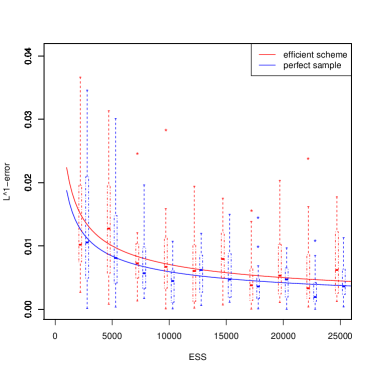
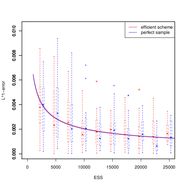
$1$st quartile of the target:	$3$rd quartile of the target:

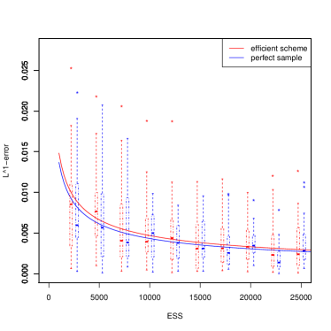
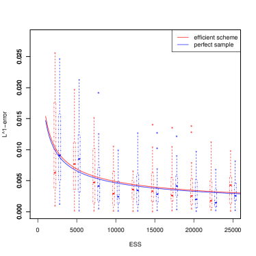
Figure 1: Comparison between errors associated to our self-calibrated and to the rejection algorithms. We estimate four functionals of the target: the mean (top left), the median (top right), the $1$st and the $3$rd quartile (bottom left and right). Each boxplot represents the variation of the $L^{1}$-error over $20$ independent replicates for values of ESS$\approx 2\,500,\ 5\,000,\ldots,\ 25\,000$. The continuous curves result from a linear fit of the $L^{1}$-error against $1/\sqrt{ESS}$ over the whole 200 independent runs.

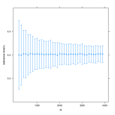
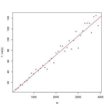
Figure 2: Numerical stability of the calibration obtained after the $1$st iteration. Top: $0.95\%$ intervals for the calibrated tolerance level $\varepsilon_{2}$. Bottom: inverse of $\varepsilon_{2}$’s variance. Variances and confidence intervals were computed on 250 independent replicates.

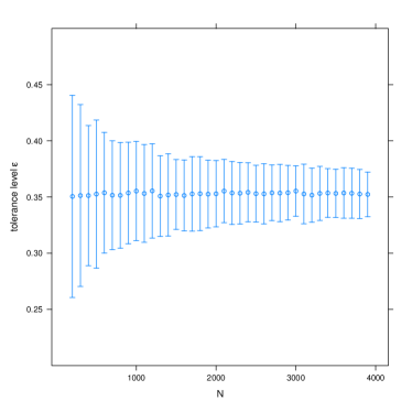
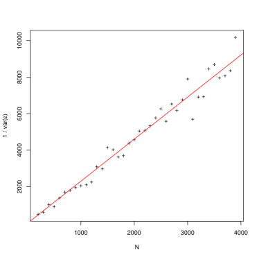
Figure 3: Numerical stability of the calibration obtained after the $8$th iteration. Top: $0.95\%$ intervals for the calibrated tolerance level $\varepsilon_{9}$. Bottom: inverse of $\varepsilon_{9}$’s variance. Variances and confidence intervals were computed on 250 independent replicates.

The following toy example, due to Sisson et al (2007), consists of a simple mixture of two univariate Gaussian distributions with unknown common mean $\boldsymbol{\theta}$ and variances equal to $1$ and $0.01$ respectively:

$$f\big{(}\mathbf{x}|\boldsymbol{\theta}\big{)}=\varphi(\mathbf{x}-\boldsymbol{\theta})/2+10\varphi\big{(}10(\mathbf{x}-\boldsymbol{\theta})\big{)}/2$$ (8)

The prior distribution on $\boldsymbol{\theta}$ is uniformly distributed over the interval $[-10,10]$. For the observation $\mathbf{x}_{\text{obs}}=0$, the posterior is

$$\pi(\boldsymbol{\theta}|\mathbf{x}_{\text{obs}}=0)\propto\big{[}\varphi(\boldsymbol{\theta})+10\varphi\big{(}10\,\boldsymbol{\theta})\big{]}\mathbf{1}\big{\{}-10\leq\boldsymbol{\theta}\leq 10\big{\}}.$$ (9)

This example is simple enough to compare sampling schemes among them and with the true posterior.

$\triangleright{}$ Is the ESS a good assessement of quality? We now have to test whether or not the accuracy of the output of an algorithm with an ESS of $n_{\text{final}}$ is comparable to a perfect sample of size $n_{\text{final}}$ drawn from the target. For this purpose, on $200$ independent runs of the efficient scheme, we evaluated the errors resulting from using the output of our algorithm to evaluate functionals of the target. We compare those with the errors associated with perfect samples. Fig. 1 studies four functionals of the target: the mean, the median, the $1$st and the $3$rd quartiles. In all cases, the differences on the error of both schemes is much smaller than the differences on the error of independent replicates of both schemes. There is almost no dissimilarity for estimates of the median and of $1$st and $3$rd quartiles. We note that the interval bounded by these last two statistics provides an ABC approximation of the credible interval with probability $1/2$, relevance of estimating them correctly.

Table 1: Comparison of ABC samplers

	Cost	ESS
Drovandi and Pettitt (2011)	$109\times 10^{5}$	$32000$
Del Moral et al (2012a)	$46\times 10^{5}$	$29250$
ABC rejection	$37\times 10^{5}$	$33285$
Our self-calibrated sampler	$23\times 10^{5}$	$33285$

The target of the above four schemes is fixed at tolerance level $\epsilon=0.09$. Cost is evaluated in term of numbers of simulations from the model (8). As shown in the third column, algorithms were tuned to produce outputs with about the same quality in term of effective sample size (ESS).

$\triangleright{}$ Comparison with other samplers. In Tab. 1, we compare four algorithms, namely those of Drovandi and Pettitt (2011), Del Moral et al (2012a) when using $M=1$ data set per particles, the rejection sampler (Alg. 1) and our proposal. In all cases, the target has tolerance level $\epsilon=0.09$. Our proposal was tuned with $N=10^{5}$ particles at the sequential stage. The other samplers were tuned to produce a sample with the same accuracy in term of ESS and tolerance level. The scheme of Del Moral et al (2012a) was disavantaged by attaching only $M=1$ simulated data set per particles, since their calibration was designed for larger values of $M$. As seen from Tab. , our sampler needs to reach the required accuracy less simulations from the model than the other three ones.

$\triangleright{}$ Stability of the calibration. We also study the numerical stability of the calibration scheme based on 250 independent replications of the whole algorithm, when the tuning parameter $N$ (ie the size of the array during the sequential stage) varies from $200$ to $4000$. Fig. 2 and 3 detail the stability of the $1$st and $8$th iteration. They indicate that the variance of the calibrated tolerance levels is of order $1/N$. Here, values of $N$ are artificially small to allow us to perform 250 replicates of the whole scheme. The typical values of $N$ we had in mind when designing the algorithm are around $10\,000$ or $100\,000$. Results of Fig. 2 and 3 indicate that the calibrated $\epsilon_{t}$’s have a tendency to converge to a fixed value with $N$, with a mean square error of order $1/N$.

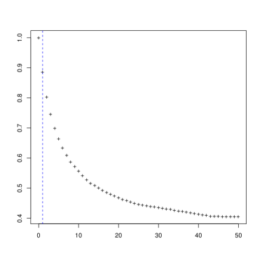
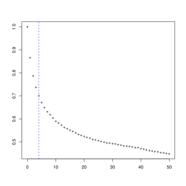
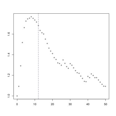
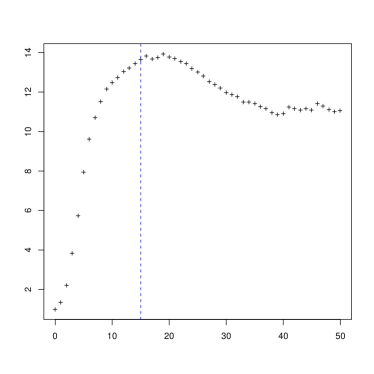
Figure 4: Efficiency of our self calibrated scheme. In all plots, $x$-axis: number of iteration and $y$-axis: the gain factor defined in Paragraph 4.1. The stopping times given by the criterion described in Paragraph 3.3 are represented by the dotted vertical lines. Top, left: uniform prior on $[-0.1,0.1]$ and $\alpha_{0}=1/10$. Top, right: uniform prior on $[-1;1]$ and $\alpha_{0}=1/10$. Bottom, left: uniform prior on $[-10,10]$ and $\alpha_{0}=1/2$. Bottom, right: uniform prior on $[-100,100]$ and $\alpha_{0}=1/4$.

$\triangleright{}$ Efficiency with respect to the gap between the prior and the posterior. We mentioned earlier (in Remark 7 and at the end of Paragraph 3.1) that sequential schemes are not recommended when the prior provides sufficient information about the parameter. The four curves in Fig. 4 correspond to various priors on the parameter $\boldsymbol{\theta}$ in Eq. (8). They show the evolution of the gain factor introduced in (7) over the iterations. The vertical dotted line (blue) indicates the stopping time given by the criterion of Paragraph 3.3. The top two curves of Fig. 4 correspond to the two most informative priors. In such cases, the stopping criterion is met in the early iterations and the efficiency is not in favor of sequential schemes. In each of the four studies, we tuned the initialisation stages to end with values of $\alpha_{0}$ equal to $1/10$, $1/10$, $1/2$, $1/4$ respectively. The two bottom curves in Fig. 4 indicate that, at least on this toy example, the efficiency of our proposal increases with the difference between prior and posterior. Thus, we conclude that our scheme can significantly save time (over the rejection algorithm) when the prior provides little information compared to the information carried by the data.

4.3 A population genetics example

We now consider an experiment that relates more directly to the genesis of ABC, namely population genetics. We perform Bayesian inference over the parameters of the evolutionary scenario (Fig. 5) of Apis mellifera (the common bee). The parameter of interest includes five dates of inter-populational events, $t_{1},\ldots,t_{5}$ (from the oldest to the newest). It is composed of two types of events: three divergences parameterized by their dates $t_{1},t_{2},t_{4}$ and two admixtures parameterized by their dates $t_{3},t_{5}$ and rates $r_{1}$ and $r_{2}$. The old, native area of Apis mellifera was Asia. Those bees invaded western Europe, bypassing the Alps going either North or South. The split between the two lineages is modelised by the divergence at time $t_{1}$. The current population in Italy (Population 2) came from an old mixture (at time $t_{3}$) from both lineages. The admixture rate $r_{1}$ and $r_{2}$ were respectively the frequency of A.m. carnica in Italy and A.m. mellifera in Aosta Valley at the foundation of the colony.

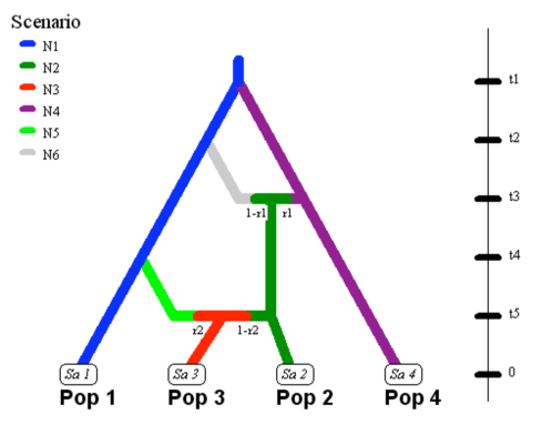
Figure 5: Evolutionary scenario of Apis mellifera. Populations 1, 2, 3 and 4 are respectively in (1) the West coast of France, (2) Italy, (3) Aosta Valley in the Alps and (4) Croatia. Populations 1, 2 and 4 represents respectively subspecies A. m. mellifera, A. m. ligustica and A. m. carnica. Meanwhile Population 3, in the area of A. m. mellifera, had been mixed recently with A.m. ligustica by beekeepers.

The data set is composed of present-day genetic data on samples of individuals collected from the four populations at the bottom of the scenario. Each sample is composed of about forty diploid individuals, and to obtain the data, each individual has been genotyped at eight microsatellite loci in the autosomal part of the genome. The eight loci might be considered as neutral (no selection pressure) and independent. To perform the ABC analysis, we computed $30$ summary statistics on the genetic data, see Appendix B.

The stochastic model is as follows: a unit time represent one generation, which is about 24 monthes for Apis mellifera. The genealogy of the sample at the $\ell$-th locus is distributed according to a coalescence process, contrained by the evolutionary scenario of Fig. 5 (Donnelly and Tavaré, 1995) This random genealogy is parameterised by the five dates $t_{1},\ldots,t_{5}$, both admixture rates $r_{1},r_{2}$ and the effective population sizes $N_{1},\ldots,N_{6}$ over the branches of the scenario as given in Fig. 5. Conditionally on that genealogy, the microsattelite marker evolves along the branches of that tree according to the generalised stepwise model (Estoup et al, 2002). This mutational process on the length of the marker is the superimposition of two independent models: the first model is composed of single nucleotide indels that occur at rate $\mu_{SNI,\ell}$ and the second model is composed of insertion or deletion of a random number, say $G$, of the repeated motif of that locus, and occurs at rate $\mu_{MIC,\ell}$. The random variable $G$ follows a geometrical distribution with parameter $0.42$.

$\triangleright$ Prior. We have built a hierarchical model on the parameters of the model. The parameter of interest (we denote it by $\phi$ to avoid confusion with the fact that the letter $\boldsymbol{\theta}$ is reserved for another use in population genetics) is made of eigth parameters: $\phi=(\widetilde{N},t_{1},t_{2},t_{3},t_{4},t_{5},r_{1},r_{2})$.

• The effective population sizes are managed by the hyper-parameter $\widetilde{N}$ with a uniform prior over $[5,100\,000]$. The six population sizes $N_{k}$, $k=1,\ldots,6$, were drawn independently from a Gamma distribution with position and shape respectively equal to $\widetilde{N}/2$ and $2$, and truncated to be in $[1,500\,000]$.

• The admixture rates $r_{1}$ and $r_{2}$ have independent uniform priors on $[0.01,0.999]$.

• The prior on the six event dates ensures that $t_{1}\geq t_{2}\geq t_{3},\ t_{4}\geq t_{5}$ and is given by:

  $$t_{5} \sim\mathcal{U}_{[0.01,800]}\,,$$

  $$(t_{4}-t_{5}) \sim\mathcal{U}_{[0,50\,000]}\,,$$

  $$(t_{3}-t_{5}) \sim\mathcal{U}_{[0,50\,000]}\,,$$

  $$t_{2}-\max\big{(}t_{3},t_{4}\big{)} \sim\mathcal{U}_{[100,500\,000]}\,,$$

  $$(t_{1}-t_{2}) \sim\mathcal{U}_{[100,2\,000\,000]}\,.$$

• At last, the mutation model is managed by fixed hyper-parameters: $\widetilde{\mu}_{SNI}=10^{-6}$ and $\widetilde{\mu}_{MIC}=10^{-4}$. The rates at the $\ell$-th locus are then drawn as

  $$\mu_{SNI,\ell} \sim{\Gamma}_{\text{trunc}}(\widetilde{\mu}_{SNI}\big{/}2,\ 2,\ 10^{-9},\ 10^{-3}),$$

  $$\mu_{MIC,\ell} \sim{\Gamma}_{\text{trunc}}(\widetilde{\mu}_{MIC}\big{/}2,\ 2,\ 5\times 10^{-7},\ 5\times 10^{-2}),$$

  where $\Gamma_{\text{trunc}}(p,\ s,\ a,\ b)$ is the Gamma distribution with position $p$, shape $s$ truncated on the interval $[a;b)$.

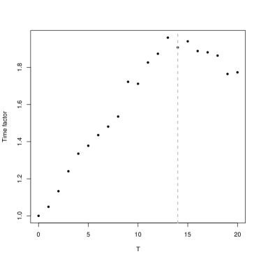
Figure 6: Efficiency of our self-calmibrated scheme estimated the gain factor in the population genetics example.

Fig. 7 shows the ABC posterior of both admixture rates. Finally, the gain factor of our proposal compared to the standard ABC rejection agorithm is given in Figure 6. The dashed vertical line indicates the stopping time of the iterative algorithm (i.e., the first $T$ for which $\rho_{T}\leq 0.1$) that is equal to $14$ iterations in the five independent replicates. We only need half the number of simulations from the model to obtain results similar to those of the standard ABC accept-reject algorithm.

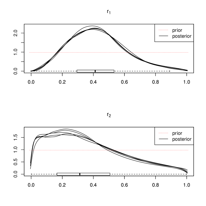
Figure 7: Stability of the estimated posterior densities for the two admixture rates on five independent replicates of our self-calibrated scheme.

5 Discussion

The paper proposes a likelihood-free, sequential algorithm calibrated in such a way as to use a relatively small number of simulations from the model while maintaining a suitable level of accuracy. In the complex example from population genetics, the SMC algorithm is about twice faster than the simple rejection algorithm. Present advances in microbiology increase the number of loci in the genetic data sets, and then the amount of information in the data, but slow down generating simulated data sets with the same number of loci in ABC algorithms. For instance, with the next generation sequencing (NGS), geneticians should be able to produce thousands of SNPs’ loci. An efficient self-calibrated sampler is a promising way to treat such large data sets if the number of summary statistics does not increase.

Throughout the paper we have left the size $N$ of the array in the sequential stage as a free parameter but it could be helpful for the user to provide guidelines on how to tune that parameter. Actually, the size should depend on the value of the final level $\epsilon_{T}$ and its distance from the tolerance level $\epsilon$ of the final target. If $\epsilon_{T}$ is not small enough, the rejection in the post-processing stage fixes the size of the very final output, which can be drastically lower than $N$. Because neither $T$ nor $\epsilon_{T}$ are known in advance, tuning $N$ is a difficult question. Our recommendation is to perform a preliminary but complete run of the whole algorithm with a value of $N$ intentionally too small (less than a thousand) to get rough estimates of $T$ and $\epsilon_{T}$ and restart the algorithm with a suitable value of $N$.

In addition, we did not provide a formal proof that our calibrating scheme do not bias the naïve sequential Monte Carlo scheme, whose correctness is already given in the literature. But we have tried to provide informal arguments in favor of our algorithm, and tested them in numerical experiments. A formal theoretical study of the proposal seems like a major challenge to us, because of the resampling steps and estimation of additional quantities for calibrating the tolerance levels.

Other important issues were set aside in this paper, like constructing or choosing the summary statistics, tuning the final tolerance level. For instance, one could adapt the efficient sequential algorithm to include an automatic construction of the summary statistics as in Fearnhead and Prangle (2012). At last, the efficient scheme deals with parameter estimation, and not with model choice. Whether or not we can provide an efficient sampler to perform a Bayesian model choice, inspired from the proposal of the paper, is still on open question.

Appendix A – Proof of the approximation in Eq. (5)

On average, the number of different particles after the resampling is $\alpha_{t}\mathbb{E}(n_{t})$. The Markov evolution of the copies might add new particles, and remove old ones. The Markov move is applied to each particle of the array of size $N$, and displace them with probability $\rho_{t}$. Thus, on average, the Markov evolution add $\rho_{t}N$ particles.

Moreover, old particles might disappear if all their copies are displaced by the Markov kernel. The probability that this occur depends on the number of copies. This number is always larger than $\ell_{t}:=N/(\alpha_{t}N)$ because each kept particle is copied $\ell_{t}$ times during the last residual resampling. Hence an old (but kept) particle is removed with probability smaller than $\rho_{t}^{\ell_{t}}$, and the expected number of old particles that disappear because of the Markov moves might then be bounded from below by $\rho_{t}^{\ell_{t}}\alpha_{t}\mathbb{E}(n_{t})=o(\alpha_{t})\mathbb{E}(n_{t})$. Morover, $\rho_{t}^{\ell_{t}}$ is negligible in front of the other terms because $\alpha_{t}\ll 1$, i.e., $\ell_{t}\gg 1$. Hence,

$$\mathbb{E}(n_{t+1})\geq(\alpha_{t}+\rho_{t}+o(\alpha_{t}))\mathbb{E}(n_{t}).$$

Appendix B – Summary statistics of the population genetic experiment

Sixteen statistics are computed within each sample: the average (over each locus) of the numbers of alleles, the average of the variances of the allele lengths, the average of the heterozygosity, the average of the M index of Garza and Williamson. Twelve statistics are computed on each pair of samples: the average of the Weir and Cockerham’s $F_{st}$ and the average of the $(\delta\mu)^{2}$ of Goldstein. The last two statistics are a rough estimate of the frequency of individuals in Population 3 that are most likely to come from Population 1 than Population 2, and a rough estimate of the frequency of individuals in Population 2 that are most likely to come from Population 4 than Population 1. Thoses statistics were computed as in the DIYABC software of Cornuet et al (2008).

References

- Beaumont (2010) Beaumont MA (2010) Approximate Bayesian Computation in Evolution and Ecology. Annu Rev Ecol Evol Syst 41:379–406
- Beaumont et al (2009) Beaumont MA, Cornuet JM, Marin JM, Robert CP (2009) Adaptive approximate Bayesian computation. Biometrika 96(4):983–990
- Cappé et al (2004) Cappé O, Guillin A, Marin JM, Robert CP (2004) Population Monte Carlo. J Comput Graph Statist 13(4):907–929
- Cornuet et al (2008) Cornuet JM, Santos F, Beaumont M, Robert CP, Marin JM, Balding D, Guillemaud T, Estoup A (2008) Infering population history with DIY ABC: a user-friedly approach Approximate Bayesian Computation. Bioinformatics 24(23):2713–2719
- Csillèry et al (2010) Csillèry K, Blum M, Gaggiotti O, François O (2010) Approximate Bayesian Computation (ABC) in practice. Trends in Ecology and Evolution 25(7):410–418
- Del Moral (2004) Del Moral P (2004) Feynman-Kac formulae. Probability and its Applications (New York), Springer-Verlag, New York, genealogical and interacting particle systems with applications
- Del Moral et al (2006) Del Moral P, Doucet A, Jasra A (2006) Sequential Monte Carlo samplers. J R Stat Soc Ser B Stat Methodol 68(3):411–436
- Del Moral et al (2012a) Del Moral P, Doucet A, Jasra A (2012a) An adaptive sequential Monte Carlo method for approximate Bayesian computation. Stat Comput 22(5):1009–1020
- Del Moral et al (2012b) Del Moral P, Doucet A, Jasra A (2012b) On adaptive resampling strategies for sequential monte carlo methods. Bernoulli 18(1):252–278
- Donnelly and Tavaré (1995) Donnelly P, Tavaré S (1995) Coalescents and genealogical structure under neutrality. Annu Rev Genet 29:401–421
- Douc et al (2005) Douc R, Cappé O, Moulines E (2005) Comparison of resampling schemes for particle filtering. In: Proceedings of the 4th International Symposium on Image and Signal Processing and Analysis (ISPA), IEEE
- Doucet et al (2001) Doucet A, de Freitas N, Gordon N (eds) (2001) Sequential Monte Carlo methods in practice. Statistics for Engineering and Information Science, Springer-Verlag, New York