Recent advances in ambit stochastics with a view towards tempo-spatial stochastic volatility/intermittency

Abstract

Ambit stochastics is the name for the theory and applications of ambit fields and ambit processes and constitutes a new research area in stochastics for tempo-spatial phenomena. This paper gives an overview of the main findings in ambit stochastics up to date and establishes new results on general properties of ambit fields. Moreover, it develops the concept of tempo-spatial stochastic volatility/intermittency within ambit fields. Various types of volatility modulation ranging from stochastic scaling of the amplitude, to stochastic time change and extended subordination of random measures and to probability and Lévy mixing of volatility/intensity parameters will be developed. Important examples for concrete model specifications within the class of ambit fields are given.

Keywords: Ambit stochastics, random measure, Lévy basis, stochastic volatility, extended subordination, meta-times, non-semimartingales.
 
MSC codes: 60G10, 60G51, 60G57, 60G60,

1 Introduction

Tempo-spatial stochastic models describe objects which are influenced both by time and location. They naturally arise in various applications such as agricultural and environmental studies, ecology, meteorology, geophysics, turbulence, biology, global economies and financial markets. Despite the fact that the aforementioned areas of application are very different in nature, they pose some common challenging mathematical and statistical problems. While there is a very comprehensive literature on both time series modelling, see e.g. Hamilton (1994); Brockwell & Davis (2002), and also on modelling purely spatial phenomena, see e.g. Cressie (1993), tempo-spatial stochastic modelling has only recently become one of the most challenging research frontiers in modern probability and statistics, see Finkenstädt et al. (2007); Cressie & Wikle (2011) for textbook treatments. Advanced and novel methods from statistics, probability, and stochastic analysis are called for to address the difficulties in constructing and estimating flexible and, at the same time, parsimoniously parametrised stochastic tempo-spatial models. There are various challenging issues which need to be addressed when dealing with tempo-spatial data, starting from data collection, model building, model estimation and selection, and model validation up to prediction. This paper focuses on building a flexible, dynamic tempo-spatial modelling framework, in which we develop the novel concept of tempo-spatial stochastic volatility/intermittency which allows one to model random volatility clusters and fluctuations both in time and in space. Note that intermittency is an alternative name for stochastic volatility, used in particular in turbulence. The presence of stochastic volatility is an empirical fact in a variety of scientific fields (including the ones mentioned above), see e.g. Amiri (2009); Huang et al. (2011); Shephard & Andersen (2009). Despite its ubiquitousness and importance, however, this important quantity has so far been often overlooked in the tempo-spatial literature. Possibly this is due to the fact that stochastic volatility induces high mathematical complexity which is challenging both in terms of model building as well as for model estimation.

The concept of stochastic volatility needs to be defined with respect to a base model, which we introduce in the following. While the models should be the best realistic description of the underlying random phenomena, they also have to be treatable for further use in the design of controls, or risk evaluation, or planning of engineering equipment in the areas of application in which the tempo-spatial phenomenon is considered. Stochastic models for such tempo-spatial systems are typically formulated in terms of evolution equations, and they rely on the use of random fields. We focus on such random fields which are defined in terms of certain types of stochastic integrals with respect to random measures which can be regarded as a unifying framework which encompasses many of the traditional modelling classes. We will work with random fields denoted by $Y_{t}({\bf x})\in\mathbb{R}$ with $Y_{t}({\bf x}):=Y({\bf x},t)$, where $t\in\mathbb{R}$ denotes the temporal parameter and ${\bf x}\in\mathbb{R}^{d}$ denotes the spatial parameter, where $d\in{I\!\!N}_{0}$. Typically, we have $d\in\{1,2,3\}$ representing, for instance, longitude, latitude and height. Note that by choosing continuous parameters $({\bf x},t)$, we can later allow for considerable flexibility in the discretisation of the model (including in particular the possibility of irregularly spaced data). This maximises the potential for wide applications of the model. We expect that the random variables $Y_{t}({\bf x})$ and $Y_{t^{\prime}}({\bf x}^{\prime})$ are correlated as soon as the points $({\bf x},t)$ and $({\bf x}^{\prime},t^{\prime})$ are “proximate” according to a suitable measure of distance. This idea can be formalised in terms of a set $A_{t}({\bf x})\subseteq\mathbb{R}^{d}\times\mathbb{R}$ such that for all $({\bf x}^{\prime},t^{\prime})\in A_{t}({\bf x})$, the random variables $Y_{t}({\bf x})$ and $Y_{t^{\prime}}({\bf x}^{\prime})$ are correlated. The set $A_{t}({\bf x})$ is sometimes referred to as causality cone and more recently as ambit set, see Barndorff-Nielsen & Schmiegel (2004), describing the sphere of influence of the random variable $Y_{t}({\bf x})$. A concrete example of an ambit set would, for instance, be given by a light cone or a sound cone.

As the base model for a tempo-spatial object, we choose

$$Y_{t}({\bf x})=\int_{A_{t}({\bf x})}h({\bf x},t;{\boldsymbol{\xi}},s)L(d{\boldsymbol{\xi}},ds),$$ (1)

where $L$ is an infinitely divisible, independently scattered random measure, i.e. a Lévy basis. Under suitable regularity conditions, our base model (1) can be linked to solutions of certain types of stochastic partial differential equations, which are often used for tempo-spatial modelling, see Barndorff-Nielsen, Benth & Veraart (2011) for details. The kernel function $h:\mathbb{R}^{d}\times\mathbb{R}\times\mathbb{R}^{d}\times\mathbb{R}\to\mathbb{R}$ needs to satisfy some integrability conditions to ensure the existence of the integral, which we will study in detail in Section 2. Note that the covariance structure of the base model is fully determined by the choice of the kernel function $h$ and the set $A_{t}({\bf x})$, see Barndorff-Nielsen et al. (2010). In particular, by choosing a certain bounded set $A_{t}({\bf x})$, one can easily construct models which induce a covariance structure with bounded support; such models are typically sought after in applications, which feature a certain decorrelation time and distance. Under suitable regularity assumptions on $h$ and on $A_{t}({\bf x})$, see Barndorff-Nielsen, Benth & Veraart (2011), the random field defined in (1) will be made stationary in time and homogeneous in space. It should be noted that in any concrete application, one needs to account for components in addition to the base model, such as a potential drift, trend and seasonality, and observation error on the data level.

One of the key questions we try to answer in this paper is the following one: How can stochastic volatility/intermittency be introduced in our base model (1)? We propose four complementary methods for tempo-spatial volatility modulation. First, stochastic volatility can be introduced by stochastically changing the amplitude of the Lévy basis $L$. This can be achieved by adding a stochastic integrand to the base model. This method has frequently been used in the purely temporal case to account for volatility clusters. In the tempo-spatial case, one needs to establish a suitable stochastic integration theory, which allows for stochastic integrands in the form of random fields. Moreover, suitable models for tempo-spatial stochastic volatility fields need to be developed.

In the purely temporal, examples typically used to model stochastic volatility are e.g. constant elasticity of variance processes, in particular, square root diffusions, see Cox (1975); Cox et al. (1985), Ornstein-Uhlenbeck (OU) processes, see Uhlenbeck & Ornstein (1930) and more recently Barndorff-Nielsen & Shephard (2001), and supOU processes, see Barndorff-Nielsen (2000); Barndorff-Nielsen & Stelzer (2011). Second, stochastic volatility can be introduced by extended subordination of the Lévy basis. This concept can be viewed as an extension of the concept of stochastic time change as developed by Bochner (1949), see also Veraart & Winkel (2010) for further references, to a tempo-spatial framework. Last, volatility modulation can be achieved by randomising a volatility/intensity parameter of the Lévy basis $L$. Here we will study both probability mixing and the new concept of Lévy mixing, which has recently been developed by Barndorff-Nielsen, Perez-Abreu & Thorbjørnsen (2012). We will show how these two mixing concepts can be used to account for stochastic volatility/intermittency.

Altogether, this paper contributes to the area of ambit stochastics, which is the name for the theory and application of ambit fields and ambit processes. Ambit stochastics is a new field of mathematical stochastics that has its origin in the study of turbulence, see e.g. Barndorff-Nielsen & Schmiegel (2004), but is in fact of broad applicability in science, technology and finance, in relation to modelling of spatio-temporal dynamic processes. E.g. important applications of ambit stochastics include modelling turbulence in physics, see e.g. Barndorff-Nielsen & Schmiegel (2004, 2009); Hedevang (2012), modelling tumour growth in biology, see Barndorff-Nielsen & Schmiegel (2007); Jónsdóttir et al. (2008), and applications in financial mathematics, see Barndorff-Nielsen, Benth & Veraart (2012); Veraart & Veraart (2012); Barndorff-Nielsen et al. (2010).

The outline for the remainder of this article is as follows. Section 2 reviews the concept of Lévy bases and integration with respect to Lévy bases, where the focus is on the integration theories developed by Rajput & Rosinski (1989) and Walsh (1986). Integrals with respect to Lévy bases are then used to establish the notion for our base model (1) and for general ambit fields and ambit processes in Section 3. In addition to reviewing the general framework of ambit fields, we establish new smoothness and semimartingale conditions for ambit fields. An important sub-class of ambit fields – the so-called trawl processes, which constitute a class of stationary infinitely divisible stochastic processes – are then presented in Section 4. Section 5 focuses on volatility modulation and establishes four complementary concepts which can be used to model tempo-spatial stochastic volatility/intermittency: Stochastic scaling of the amplitude through a stochastic integrand, time change and extended subordination of a random measure, and probability and Lévy mixing. Finally, Section 6 concludes and gives an outlook on future research.

2 Background

Ambit fields and ambit processes are constructed from so-called Lévy bases. We will now review the definition and key properties of such Lévy bases and then describe how stochastic integrals can be defined with respect to Lévy bases.

2.1 Background on Lévy bases

Our review is based on the work by Rajput & Rosinski (1989); Pedersen (2003), where detailed proofs can be found.

Throughout the paper, we denote by $(\Omega,\mathcal{F},P)$ a probability space. Also, let $(S,\mathcal{S},\mathit{L}eb)$ denote a Lebesgue-Borel space where $S$ denotes a Borel set in $\mathbb{R}^{k}$ for a $k\in\mathbb{N}$, e.g. often we choose $S=\mathbb{R}^{k}$. Moreover $\mathcal{S}=\mathcal{B}(S)$ is the Borel $\sigma$-algebra on $S$ and $\mathit{L}eb$ denotes the Lebesgue measure. In addition, we define

$$\mathcal{B}_{b}(S)=\{A\in\mathcal{S}:\mathit{L}eb(A)<\infty\},$$

which is the subset of $\mathcal{S}$ that contains sets which have bounded Lebesgue measure. Note that since $\mathit{L}eb$ is $\sigma$-finite, we can deduce that $\mathcal{S}=\sigma(\mathcal{B}_{b}(S))$, see Peccati & Taqqu (2008, p. 399). Also, the set $\mathcal{B}_{b}(S)$ is closed under finite union, relative complementation, and countable intersection and is therefore a $\delta$-ring.

2.1.1 Random measures

Random measures play a key role in ambit stochastics, hence we start off by recalling the definition of a (full) random measure.

Definition 1.

1. By a random measure $M$ on $(S,\mathcal{S})$ we mean a collection of $\mathbb{R}$-valued random variables $\left\{M\left(A\right):A\in\mathcal{B}_{b}(S)\right\}$ such that for any sequence $A_{1},A_{2},\dots$ of disjoint elements of $\mathcal{B}_{b}(S)$ satisfying $\cup_{j=1}^{\infty}A_{j}\in\mathcal{B}_{b}(S)$ we have $M\left(\cup_{j=1}^{\infty}A_{j}\right)=\sum_{j=1}^{\infty}M\left(A_{j}\right)$ a.s..

2. By a full random measure $M$ on $(S,\mathcal{S})$  we mean a random object whose realisations are measures on $(S,\mathcal{S})$ a.s..

Note here that a realisation of a random measure is in general not an ordinary signed measure since it does not necessarily have finite variation. That is why we also introduced the term of a full random measure. Other articles or textbooks would sometimes call the quantity we have defined as a random measure as random noise to stress that it might not be a (signed) measure, see Samorodnitsky & Taqqu (1994, p. 118) for a discussion of this aspect.

In some applications, we work with stationary random measures, which are defined as follows.

Definition 2.

A (full) random measure on $\mathcal{S}$ is said to be stationary if for any ${\bf s}\in S$ and any finite collection $A_{1},A_{2},\dots,A_{n}$ of elements (of $\mathcal{B}(S)$) of $\mathcal{B}_{b}(\mathcal{S})$ the random vector

$$\left(M\left(A_{1}+{\bf s}\right),M\left(A_{2}+{\bf s}\right),\dots,M\left(A_{n}+{\bf s}\right)\right)$$

has the same law as $\left(M\left(A_{1}\right),M\left(A_{2}\right),\dots,M\left(A_{n}\right)\right)$.

The above definition ensures that a random measure is stationary in all components. One could also study stationarity in the individual components separately.

2.1.2 Lévy bases

In this paper, we work with a special class of random measures, called Lévy bases. Before we can define them, we define independently scattered random measures.

Definition 3.

A random measure $M$ on $(S,\mathcal{S})$ is independently scattered if for any sequence $A_{1},A_{2},\dots$ of disjoint elements of $\mathcal{B}_{b}(S)$, the random variables $M(A_{1}),M(A_{2}),\dots$ are independent.

Recall the definition of infinite divisibility of a distribution.

Definition 4.

The law $\mu$ of a random variable on $\mathbb{R}$ is infinitely divisible (ID) if for any $n\in{I\!\!N}$, there exists a law $\mu_{n}$ on $\mathbb{R}$ such that $\mu=\mu_{n}^{*n}$, where $\mu_{n}^{*n}$ denotes the $n$-fold convolution of $\mu_{n}$ with itself.

In the following, we are interested in ID random measures, which we define now.

Definition 5.

A random measure $M$ on $(S,\mathcal{S})$ is said to be infinitely divisible if for any finite collection $A_{1},A_{2},\dots,A_{n}$ of elements of $\mathcal{B}_{b}(S)$ the random vector $\left(M\left(A_{1}\right),M\left(A_{2}\right),\dots,M\left(A_{n}\right)\right)$ is infinitely divisible.

Let us study one relevant example.

Example 1.

Assume that $M$ is an absolutely continuous full random measure on $(S,\mathcal{S})$ with a density $m$ and suppose that the stochastic process $\left\{m\left(x\right)\right\}_{x\in S}$ is non-negative and infinitely divisible. Then $M$ is an infinitely divisible full random measure.

Now we can give the definition of a Lévy basis.

Definition 6.

1. A Lévy basis $L$ on $(S,\mathcal{S})$ is an independently scattered, infinitely divisible random measure.

2. A homogeneous Lévy basis on $(S,\mathcal{S})$ is a stationary, independently scattered, infinitely divisible random measure.

2.1.3 Lévy-Khintchine formula and Lévy-Itô decomposition

Since a Lévy basis $L$ is ID, it has a Lévy-Khintchine representation. I.e. let $\zeta\in\mathbb{R}$ and $A\in\mathcal{B}_{b}(S)$, then

$$\begin{split}C\{\zeta\ddagger L(A)\}&=\log\left(\mathbb{E}(\exp(i\zeta L(A))\right)\\ &=i\zeta a^{*}(A)-\frac{1}{2}\zeta^{2}b^{*}(A)+\int_{\mathbb{R}}\left(e^{i\zeta x}-1-i\zeta x\mathbb{I}_{[-1,1]}(x)\right)n(dx,A),\end{split}$$ (2)

where, according to Rajput & Rosinski (1989, Proposition 2.1 (a)), $a^{*}$ is a signed measure on $\mathcal{B}_{b}(S)$, $b^{*}$ is a measure on $\mathcal{B}_{b}(S)$, and $n(\cdot,\cdot)$ is the generalised Lévy measure, i.e. $n(dx,A)$ is a Lévy measure on $\mathbb{R}$ for fixed $A\in\mathcal{B}_{b}(S)$ and a measure on $\mathcal{B}_{b}(S)$ for fixed $dx$.

Next, we define the control measure as introduced in Rajput & Rosinski (1989, Proposition 2.1 (c), Definition 2.2).

Definition 7.

Let $L$ be a Lévy basis with Lévy-Khintchine representation (2). Then, the measure $c$ is defined by

$$c(B)=|a^{*}|(B)+b^{*}(B)+\int_{\mathbb{R}}\min(1,x^{2})n(dx,B),\qquad B\in\mathcal{S}_{b},$$ (3)

where $|\cdot|$ denotes the total variation. The extension of the measure $c$ to a $\sigma$-finite measure on $(S,\mathcal{S})$ is called the control measure measure of $L$.

Based on the control measure we can now characterise the generalised Lévy measure $n$ further, see Rajput & Rosinski (1989, Lemma 2.3, Proposition 2.4). First of all, we define the Radon-Nikodym derivatives of the three components of $c$, which are given by

$$a({\bf z})=\frac{da^{*}}{dc}({\bf z}), b({\bf z})=\frac{db^{*}}{dc}({\bf z}), \nu(dx,{\bf z})=\frac{n(dx,\cdot)}{dc}({\bf z}).$$ (4)

Hence, we have in particular that $n(dx,d{\bf z})=\nu(dx,{\bf z})c(d{\bf z})$. Without loss of generality we can assume that $\nu(dx,{\bf z})$ is a Lévy measure for each fixed ${\bf z}$ and hence we do so in the following.

Definition 8.

We call $(a,b,\nu(dx,\cdot),c)=(a({\bf z}),b({\bf z}),\nu(dx,{\bf z}),c(d{\bf z}))_{{\bf z}\in S}$ a characteristic quadruplet (CQ) associated with a Lévy basis $L$ on $(S,\mathcal{S})$ provided the following conditions hold:

1. Both $a$ and $b$ are functions on $S$, where $b$ is restricted to be non-negative.

2. For fixed ${\bf z}$, $\nu(dx,{\bf z})$ is a Lévy measure on $\mathbb{R}$, and, for fixed $dx$, it is a measurable function on $S$.

3. The control measure $c$ is a measure on $(S,\mathcal{S})$ such that $\int_{B}a({\bf z})c(d{\bf z})$ is a (possibly signed) measure on $(S,\mathcal{S})$, $\int_{B}b({\bf z})c(d{\bf z})$ is a measure on $(S,\mathcal{S})$ and $\int_{B}\nu(dx,{\bf z})c(d{\bf z})$ is a Lévy measure on $\mathbb{R}$ for fixed $B\in\mathcal{S}$.

We have seen that every Lévy basis on $(S,\mathcal{S})$ determines a CQ of the form $(a,b,\nu(dx,\cdot),c)=(a({\bf z}),b({\bf z}),\nu(dx,{\bf z}),c(d{\bf z}))_{{\bf z}\in S}$. And, conversely, every CQ satisfying the conditions in Definition 8 determines, in law, a Lévy basis on $(S,\mathcal{S})$ .

In a next step, we relate the notion of Lévy bases and CQs to the concept of Poisson random measures and their compensators.

Definition 9.

A Lévy basis on $(S,\mathcal{S})$ is dispersive if its control measure $c$ satisfies $c(\{{\bf z}\})=0$ for all ${\bf z}\in S$.

For a dispersive Lévy basis $L$ on $(S,\mathcal{S})$ with characteristic quadruplet $(a,b,\nu,c)$ there is a modification $L^{*}$ with the same characteristic quadruplet which has following Lévy-Itô decomposition:

$$L^{*}(A) =a^{*}(A)+W(A)+\int_{\{|y|\leq 1\}}y(N-n)(dy,A)+\int_{\{|y|>1\}}yN(dy,A),$$ (5)

for $A\in\mathcal{B}_{b}(S)$ and for a Gaussian basis $W$ (with characteristic quadruplet $(0,b,0,c)$, i.e. $W(A)\sim N(0,\int_{A}b({\bf z})c(d{\bf z}))$), and a Poisson basis $N$ (independent of $W$) with compensator $n\left(dy;A\right)=\mathrm{E}\left\{N\left(dy;A\right)\right\}$ where $n(dx,d{\bf z})=\nu(dx,{\bf z})c(d{\bf z})$, cf. Pedersen (2003) and Barndorff-Nielsen & Stelzer (2011, Theorem 2.2)

It is also possible to write (5) in infinitesimal form by

$$L^{*}(d{\bf z})=a^{*}(d{\bf z})+W(d{\bf z})+\int_{\{|x|>1\}}xN(dx,d{\bf z})+\int_{\{|x|\leq 1\}}x(N-n)(dx,d{\bf z}).$$ (6)

This is particularly useful in the context of the Lévy-Khintchine representation, which can then also be expressed in infinitesimal form by

$$\begin{split}C\{\zeta\ddagger L(d{\bf z})\}&=\log\left(\mathbb{E}(\exp(i\zeta L(d{\bf z}))\right)\\ &=i\zeta a^{*}(d{\bf z})-\frac{1}{2}\zeta^{2}b^{*}(d{\bf z})+\int_{\mathbb{R}}\left(e^{i\zeta x}-1-i\zeta x\mathbb{I}_{[-1,1]}(x)\right)n(dx,d{\bf z})\\ &=\left(i\zeta a({\bf z})-\frac{1}{2}\zeta^{2}b({\bf z})+\int_{\mathbb{R}}\left(e^{i\zeta x}-1-i\zeta x\mathbb{I}_{[-1,1]}(x)\right)\nu(dx,{\bf z})\right)c(d{\bf z})\\ &=C\{\zeta\ddagger L^{\prime}({\bf z})\}c(d{\bf z}),\qquad\zeta\in\mathbb{R},\end{split}$$ (7)

where $L^{\prime}({\bf z})$ denotes the Levy seed of $L$ at ${\bf z}$. Note that $L^{\prime}({\bf z})$ is defined as the infinitely divisible random variable having Lévy-Khintchine representation

$$C\{\zeta\ddagger L^{\prime}({\bf z})\}=i\zeta a({\bf z})-\frac{1}{2}\zeta^{2}b({\bf z})+\int_{\mathbb{R}}\left(e^{i\zeta x}-1-i\zeta x\mathbb{I}_{[-1,1]}(x)\right)\nu(dx,{\bf z}).$$ (8)

Remark 1.

We can associate a Lévy process with any Lévy seed. In particular, let $L^{\prime}({\bf z})$ denote the Lévy seed of $L$ at ${\bf z}$. Then, $(L_{t}^{\prime}({\bf z}))_{t}$ denotes the Lévy process generated by $L^{\prime}({\bf z})$, which is defined as the Lévy process whose law is determined by $L_{1}^{\prime}({\bf z})\stackrel{{\scriptstyle law}}{{=}}L^{\prime}({\bf z})$.

Definition 10.

Let $L$ denote a Lévy basis on $(S,\mathcal{S})$ with CQ given by $(a,b,\nu(dx,\cdot),c)$.

1. If $\nu(dr,{\bf z})$ does not depend on ${\bf z}$, we call $L$ factorisable.

2. If $L$ is factorisable and if $c$ is proportional to the Lebesgue measure and $a({\bf z})$ and $b({\bf z})$ do not depend on $z$, then $L$ is called homogeneous. In that case we write $c(d{\bf z})=v\mathit{L}eb(d{\bf z})=vd{\bf z}$ for a positive constant $v>0$ and where $\mathit{L}eb(\cdot)$ denotes the Lebesgue measure.

In order to simplify the exposition, we will throughout this paper assume that in the case of a homogeneous Lévy basis the constant $v$ is set to 1, i.e. the measure $c$ is given by the Lebesgue measure.

2.1.4 Examples of Lévy bases

Let us study some examples of Lévy bases $L$ on $(\mathbb{R}^{k},\mathcal{B}(\mathbb{R}^{k}))$ with CQ $(a,b,\nu(dx,\cdot),c)$.

Example 2 (Gaussian Lévy basis).

When $\nu(dx,{\bf z})\equiv 0$, then $L$ constitutes a Gaussian Lévy basis with $L(A)\sim\mathit{N}\left(\int_{A}a({\bf z})c(d{\bf z}),\int_{A}b({\bf z})c(d{\bf z})\right)$, for $A\in\mathcal{B}_{b}(\mathbb{R}^{k})$. If, in addition, $L$ is homogeneous, then $L(A)\sim\mathit{N}\left(a\mathit{L}eb(A),b\mathit{L}eb(A)\right)$.

Example 3 (Poisson Lévy basis).

When $c(d{\bf z})=d{\bf z}$ and $a\equiv b\equiv 0$ and $\nu(dx;{\bf z})=\lambda({\bf z})\delta_{1}(dx)$, where $\delta_{1}$ denotes the Dirac measure with point mass at 1 and $\lambda({\bf z})>0$ is the intensity function, then $L$ constitutes a Poisson Lévy basis. If, in addition, $L$ is factorisable, i.e. $\lambda$ does not depend on ${\bf z}$, then $L(A)\sim\mathit{Poisson}\left(\lambda\mathit{L}eb(A)\right)$, for all $A\in\mathcal{B}_{b}(\mathbb{R}^{k})$.

Example 4 (Gamma Lévy basis).

Suppose that $c(d{\bf z})=d{\bf z}$, $a\equiv b\equiv 0$ and the (generalised) Lévy measure is of the form $\nu(dx;{\bf z})=x^{-1}e^{-\alpha({\bf z})x}dx$, where $\alpha({\bf z})>0$. In that case, we call the corresponding Lévy basis $L$ a gamma Lévy basis. If, in addition, $L$ is factorisable, i.e. the function $\alpha$ does not depend on the parameter ${\bf z}$, then $L(A)$ has a gamma law for all $A\in\mathcal{B}_{b}(\mathbb{R}^{k})$.

Example 5 (Inverse Gaussian Lévy basis).

Suppose that $c(d{\bf z})=d{\bf z}$, $a\equiv b\equiv 0$ and the (generalised) Lévy measure is of the form $\nu(dx;{\bf z})=x^{-3/2}e^{-\frac{1}{2}\gamma^{2}({\bf z})x}dx$, where $\gamma({\bf z})>0$. Then we call the corresponding Lévy basis $L$ an inverse Gaussian Lévy basis. If, in addition, $L$ is factorisable, i.e. the function $\gamma$ does not depend on the parameter ${\bf z}$, then $L(A)$ has an inverse Gaussian law for all $A\in\mathcal{B}_{b}(\mathbb{R}^{k})$.

Example 6 (Lévy process).

If $k=1$, i.e. $L$ is a Lévy basis on $\mathbb{R}$, then $L([0,t])=L_{t}$, $t\geq 0$ is a Lévy process.

2.2 Integration concepts with respect to a Lévy basis

In order to build relevant models based on Lévy bases, we need a suitable integration theory. In the following, we will briefly review the integration theory developed by Rajput & Rosinski (1989) and also the one by Walsh (1986), and we refer to Barndorff-Nielsen, Benth & Veraart (2011) for a detailed overview on integration concepts with respect to Lévy bases, see also Dalang & Quer-Sardanyons (2011) for a related review and Basse-O’Connor et al. (2012) for details on integration with respect to multiparameter processes with stationary increments.

2.2.1 The integration concept by Rajput & Rosinski (1989)

According to Rajput & Rosinski (1989, p.460), integration of suitable deterministic functions with respect to Lévy bases can be defined as follows. First define an integral for simple functions:

Definition 11.

Let $L$ be a Lévy basis on $(S,\mathcal{S})$. Define a simple function on $S$, i.e. let $f:=\sum_{j=1}^{n}x_{j}\mathbb{I}_{A_{j}}$, where $A_{j}\in\mathcal{B}_{b}(S)$, for $j=1,\dots,n$, are disjoint. Then, one defines the integral, for every $A\in\sigma(\mathcal{B}_{b}(S))=\mathcal{S}$, by

$$\int_{A}fdL:=\sum_{j=1}^{n}x_{j}L(A\cap A_{j}).$$

The integral for general measurable functions can be derived by a limit argument.

Definition 12.

Let $L$ be a Lévy basis on $(S,\mathcal{S})$. A measurable function $f:(S,\mathcal{S})\mapsto(\mathbb{R},\mathcal{B}(\mathbb{R}))$ is called $L$-measurable if there exists a sequence $\{f_{n}\}$ of simple function as in Definition 11, such that

• $f_{n}\to f$ a.e. (i.e. $c$-a.e., where $c$ is the control measure of $L$),

• for every $A\in\mathcal{S}$, the sequence of simple integrals $\{\int_{A}f_{n}dL\}$ converges in probability, as $n\to\infty$.

For integrable measurable functions, define

$$\int_{A}fdL:=\mathbb{P}-\lim_{n\to\infty}\int_{A}f_{n}dL.$$

Rajput & Rosinski (1989) have pointed out that the above integral is well-defined in the sense that it does not depend on the approximating sequence $\{f_{n}\}$. Also, the necessary and sufficient conditions for the existence of the integral $\int fdL$ can be expressed in terms of the characteristics of $L$ and can be found in Rajput & Rosinski (1989, Theorem 2.7), which says the following. Let $f:(S,\mathcal{S})\mapsto(\mathbb{R},\mathcal{B}(\mathbb{R}))$ be a measurable function. Let $L$ be a Lévy basis with CQ $(a,b,\nu(dx,\cdot),c)$. Then $f$ is integrable w.r.t.  $L$ if and only if the following three conditions are satisfied:

$$\int_{S}|V_{1}(f({\bf z}),{\bf z})|c(d{\bf z})<\infty, \int_{S}|f({\bf z})|^{2}b({\bf z})c(d{\bf z})<\infty, \int_{S}V_{2}(f({\bf z}),{\bf z})c(d{\bf z})<\infty,$$ (9)

where for $\varrho(x):=x\mathbb{I}_{[-1,1]}(x)$,

$$V_{1}(u,{\bf z}):=ua({\bf z})+\int_{\mathbb{R}}\left(\varrho(xu)-u\varrho(x)\right)\nu(dx,{\bf z}), V_{2}(u,{\bf z}):=\int_{\mathbb{R}}\min(1,|xu|^{2})\nu(dx,{\bf z}).$$

Note that such integrals have been defined for deterministic integrands. However, in the context of ambit fields, which we will focus on in this paper, we typically encounter stochastic integrands representing stochastic volatility, which tends to be present in most applications we have in mind. Since we often work under the independence assumption that the stochastic volatility $\sigma$ and the Lévy basis $L$ are independent, it has been suggested to work with conditioning to extend the definition by Rajput & Rosinski (1989) to allow for stochastic integrands. An alternative concept, which directly allows for stochastic integrands which can be dependent of the Lévy basis, is the integration concept by Walsh (1986), which we study next.

2.2.2 Integration w.r.t. martingale measures introduced by Walsh (1986)

The integration theory due to Walsh (1986) can be regarded as Itô integration extended to random fields. In the following we will present the integration theory on a bounded domain and comment later on how one can extend the theory to the case of an unbounded domain.

Here we treat time and space separately, which allows us to work with a natural ordering (introduced by time) and to relate the integrals w.r.t. to Lévy bases to martingale measures. In the following, we denote by $S$ a bounded Borel set in $\mathcal{X}=\mathbb{R}^{d}$ for a $d\in\mathbb{N}_{0}$ (where $d+1=k$) and $\mathcal{S}=\mathcal{B}(S)$ denotes the Borel $\sigma$-algebra on $S$. Since $S$ is bounded, we have in fact $\mathcal{S}=\mathcal{B}(S)=\mathcal{B}_{b}(S)$.

Let $L$ denote a Lévy basis on $(S\times[0,T],\mathcal{B}(S\times[0,T]))$ for some $T>0$. For any $A\in\mathcal{B}_{b}(S)$ and $0\leq t\leq T$, we define

$$L_{t}(A)=L(A,t)=L(A\times(0,t]).$$

Here $L_{t}(\cdot)$ is a measure-valued process, and for a fixed set $A\in\mathcal{B}_{b}(S)$, $L_{t}(A)$ is an additive process in law. In the following, we want to use the $L_{t}(A)$ as integrators as in Walsh (1986). In order to do that, we work under the square-integrability assumption, i.e.:

Assumption (A1):

For each $A\in\mathcal{B}_{b}(S)$, we have that $L_{t}(A)\in L^{2}(\Omega,\mathcal{F},P)$.

In the following, we will, unless otherwise stated, work without loss of generality under the zero-mean assumption on $L$, i.e.

Assumption (A2):

For each $A\in\mathcal{B}_{b}(S)$, we have that $\mathbb{E}(L_{t}(A))=0$.

Next, we define the filtration $\mathcal{F}_{t}$ by

$$\mathcal{F}_{t}=\cap_{n=1}^{\infty}\mathcal{F}_{t+1/n}^{0}, \text{where}\qquad\mathcal{F}_{t}^{0}=\sigma\{L_{s}(A):A\in\mathcal{B}_{b}(S),0<s\leq t\}\vee\mathcal{N},$$ (10)

and where $\mathcal{N}$ denotes the $P$-null sets of $\mathcal{F}$. Note that $\mathcal{F}_{t}$ is right-continuous by construction. One can show that under the assumptions (A1) and (A2) and for fixed $A\in\mathcal{B}_{b}(S)$, $(L_{t}(A))_{0\leq t\leq T}$ is a (square-integrable) martingale with respect to the filtration $(\mathcal{F}_{t})_{0\leq t\leq T}$. Note that these two properties together with the fact that $L_{0}(A)=0$ a.s. ensure that $(L_{t}(A))_{t\geq 0,A\in\mathcal{B}(R^{d})}$ is a martingale measure with respect to $(\mathcal{F}_{t})_{0\leq t\leq T}$ in the sense of Walsh (1986). Furthermore, we have the following orthogonality property: If $A,B\in\mathcal{B}_{b}(S)$ with $A\cap B=\emptyset$, then $L_{t}(A)$ and $L_{t}(B)$ are independent. Martingale measures which satisfy such an orthogonality property are referred to as orthogonal martingale measures by Walsh (1986), see also Barndorff-Nielsen, Benth & Veraart (2011) for more details. Note that orthogonal martingale measure are worthy, see Walsh (1986, Corollary 2.9), a property which makes them suitable as integrators. For such orthogonal martingale measures, Walsh (1986) introduces their covariance measure $Q$ by

$$Q(A\times[0,t])=\ <L(A)>_{t},$$ (11)

for $A\in\mathcal{B}(S)$. Note that $Q$ is a positive measure and is used by Walsh (1986) when defining stochastic integration with respect to $L$.

Walsh (1986) defines stochastic integration in the following way. Let $\zeta(\xi,s)$ be an elementary random field $\zeta(\xi,s)$, i.e. it has the form

$$\zeta({\boldsymbol{\xi}},s,\omega)=X(\omega)\mathbb{I}_{(a,b]}(s)\mathbb{I}_{A}({\boldsymbol{\xi}})\,,$$ (12)

where $0\leq a<t$, $a\leq b$, $X$ is bounded and $\mathcal{F}_{a}$-measurable, and $A\in\mathcal{S}$. For such elementary functions, the stochastic integral with respect to $L$ can be defined as

$$\int_{0}^{t}\int_{B}\zeta({\boldsymbol{\xi}},s)\,L(d{\boldsymbol{\xi}},ds):=X\left(L_{t\wedge b}(A\cap B)-L_{t\wedge a}(A\cap B)\right)\,,$$ (13)

for every $B\in\mathcal{S}$. It turns out that the stochastic integral becomes a martingale measure itself in $B$ (for fixed $a,b,A$). Clearly, the above integral can easily be generalised to allow for integrands given by simple random fields, i.e. finite linear combinations of elementary random fields. Let $\mathcal{T}$ denote the set of simple random fields and let the predictable $\sigma$-algebra $\mathcal{P}$ be the $\sigma$-algebra generated by $\mathcal{T}$. Then we call a random field predictable provided it is $\mathcal{P}$-measurable. The aim is now to define stochastic integrals with respect to $L$ where the integrand is given by a predictable random field.

In order to do that Walsh (1986) defines a norm $\|\cdot\|_{L}$ on the predictable random fields $\zeta$ by

$$\|\zeta\|_{L}^{2}:=\mathbb{E}\left[\int_{[0,T]\times S}\zeta^{2}({\boldsymbol{\xi}},s)\,Q(d{\boldsymbol{\xi}},ds)\right]\,,$$ (14)

which determines the Hilbert space $\mathcal{P}_{L}:=L^{2}(\Omega\times[0,T]\times S,\mathcal{P},Q)$, which is the space of predictable random fields $\zeta$ with $\|\zeta\|_{L}^{2}<\infty$, and he shows that $\mathcal{T}$ is dense in $\mathcal{P}_{L}$. Hence, in order to define the stochastic integral of $\zeta\in\mathcal{P}_{L}$, one can choose an approximating sequence $\{\zeta_{n}\}_{n}\subset\mathcal{T}$ such that $\|\zeta-\zeta_{n}\|_{L}\rightarrow 0$ as $n\rightarrow\infty$. Clearly, for each $A\in\mathcal{S}$, $\int_{[0,t]\times A}\zeta_{n}({\boldsymbol{\xi}},s)\,L(d{\boldsymbol{\xi}},ds)$ is a Cauchy sequence in $L^{2}(\Omega,\mathcal{F},P)$, and thus there exists a limit which is defined as the stochastic integral of $\zeta$.

Then, this stochastic integral is again a martingale measure and satisfies the following Itô-type isometry:

$$\mathbb{E}\left[\left(\int_{[0,T]\times S}\zeta({\boldsymbol{\xi}},s)L(d{\boldsymbol{\xi}},ds)\right)^{2}\right]=\|\zeta\|_{L}^{2}\,,$$ (15)

see (Walsh, 1986, Theorem 2.5) for more details.

2.2.3 Relation between the two integration concepts

The relation between the two different integration concept has been discussed in Barndorff-Nielsen, Benth & Veraart (2011, pp. 60–61), hence we only mention it briefly here.

Note that the Walsh (1986) theory defines the stochastic integral as the $L^{2}$-limit of simple random fields, whereas Rajput & Rosinski (1989) work with the $P$-limit. Barndorff-Nielsen, Benth & Veraart (2011) point out that deterministic integrands, which are integrable in the sense of Walsh, are thus also integrable in the Rajput and Rosinski sense since the control measure of Rajput & Rosinski (1989) and the covariance measure of Walsh (1986) are equivalent.

3 General aspects of the theory of ambit fields and processes

In the following we will show how stochastic processes and random fields can be constructed based on Lévy bases, which leads us to the general framework of ambit fields. This section reviews the concept of ambit fields and ambit processes. For a detailed account on this topic see Barndorff-Nielsen, Benth & Veraart (2011) and Barndorff-Nielsen & Schmiegel (2007).

3.1 The general framework

The general framework for defining an ambit process is as follows. Let $Y=\left\{Y_{t}\left({\bf x}\right)\right\}$ with $Y_{t}({\bf x}):=Y({\bf x},t)$ denoting a stochastic field in space-time $\mathcal{X}\times\mathbb{R}$. In most applications, the space $\mathcal{X}$ is chosen to be $\mathbb{R}^{d}$ for $d=1,2$ or $3$. Let $\varpi\left(\theta\right)=\left({\bf x}\left(\theta\right),t\left(\theta\right)\right)$ denote a curve in $\mathcal{X}\times\mathbb{R}$. The values of the field along the curve are then given by $X_{\theta}=Y_{t\left(\theta\right)}\left({\bf x}\left(\theta\right)\right)$. Clearly, $X=\left\{X_{\theta}\right\}$ denotes a stochastic process. Further, the stochastic field is assumed to be generated by innovations in space-time with values $Y_{t}\left({\bf x}\right)$ which are supposed to depend only on innovations that occur prior to or at time $t$ and in general only on a restricted set of the corresponding part of space-time. I.e., at each point $\left({\bf x},t\right)$, the value of $Y_{t}\left({\bf x}\right)$ is only determined by innovations in some subset $A_{t}\left({\bf x}\right)$ of $\mathcal{X}\times\mathbb{R}_{t}$ (where $\mathbb{R}_{t}=(-\infty,t]$), which we call the ambit set associated to $\left({\bf x},t\right)$. Furthermore, we refer to $Y$ and $X$ as an ambit field and an ambit process, respectively.

In order to use such general ambit fields in applications, we have to impose some structural assumptions. More precisely, we will define $Y_{t}\left({\bf x}\right)$ as a stochastic integral plus a drift term, where the integrand in the stochastic integral will consist of a deterministic kernel times a positive random variate which is taken to express the volatility of the field $Y$. More precisely, we think of ambit fields as being defined as follows.

Definition 13.

Using the notation introduced above, an ambit field is defined as a random field of the form

$$Y_{t}\left({\bf x}\right)=\mu+\int_{A_{t}\left({\bf x}\right)}h\left({\bf x},t;{\boldsymbol{\xi}},s\right)\sigma_{s}\left({\boldsymbol{\xi}}\right)L\left(\mathrm{d}{\boldsymbol{\xi}},\mathrm{d}s\right)+\int_{D_{t}\left({\bf x}\right)}q\left({\bf x},t;{\boldsymbol{\xi}},s\right)a_{s}\left({\boldsymbol{\xi}}\right)\mathrm{d}{\boldsymbol{\xi}}\mathrm{d}s,$$ (16)

provided the integrals exist, where $A_{t}\left({\bf x}\right)$, and $D_{t}\left({\bf x}\right)$ are ambit sets, $h$ and $q$ are deterministic functions, $\sigma\geq 0$ is a stochastic field referred to as volatility or intermittency, $a$ is also a stochastic field, and $L$ is a Lévy basis.

Remark 2.

Note that compared to the base model (1) we introduced in the Introduction, the ambit field defined in (16) also comes with a drift term and stochastic volatility introduced in form of a stochastic integrand. In Section 5, we will describe in detail how such a stochastic volatility field $\sigma$ can be specified and what kind of complementary routes can be taken in order to allow for stochastic volatility clustering.

The corresponding ambit process $X$ along the curve $\varpi$ is then given by

$$X_{\theta}=\mu+\int_{A(\theta)}h(t(\theta);{\boldsymbol{\xi}},s)\sigma_{s}({\boldsymbol{\xi}})L(d{\boldsymbol{\xi}},ds)+\int_{D(\theta)}q(t(\theta);{\boldsymbol{\xi}},s)a_{s}({\boldsymbol{\xi}})d{\boldsymbol{\xi}}ds,$$ (17)

where $A(\theta)=A_{t(\theta)}({\bf x}(\theta))$ and $D(\theta)=D_{t(\theta)}({\bf x}(\theta))$.

In Section 3.2, we will formulate the suitable integrability conditions which guarantee the existence of the integrals above.

Of particular interest in many applications are ambit processes that are stationary in time and nonanticipative and homogeneous in space. More specifically, they may be derived from ambit fields $Y$ of the form

$$Y_{t}\left({\bf x}\right) =\mu+\int_{A_{t}\left({\bf x}\right)}h\left({\bf x}-{\boldsymbol{\xi}},t-s\right)\sigma_{s}\left({\boldsymbol{\xi}}\right)L\left(\mathrm{d}{\boldsymbol{\xi}},\mathrm{d}s\right)+\int_{D_{t}\left({\bf x}\right)}q\left({\bf x}-{\boldsymbol{\xi}},t-s\right)a_{s}\left({\boldsymbol{\xi}}\right)\mathrm{d}{\boldsymbol{\xi}}\mathrm{d}s.$$ (18)

Here the ambit sets $A_{t}\left({\bf x}\right)$ and $D_{t}\left({\bf x}\right)$ are taken to be homogeneous and nonanticipative, i.e. $A_{t}\left({\bf x}\right)$ is of the form $A_{t}\left({\bf x}\right)=A+\left({\bf x},t\right)$ where $A$ only involves negative time coordinates, and similarly for $D_{t}\left({\bf x}\right)$. In addition, $\sigma$ and $a$ are chosen to be stationary in time and space and $L$ to be homogeneous.

3.2 Integration for general ambit fields

Ambit fields have initially been defined for deterministic integrands using the Rajput & Rosinski (1989) integration concept. Their definition could then be extended to allow for stochastic integrands which are independent of the Lévy basis by a conditioning argument. As discussed before, the integration framework developed by Walsh (1986) has the advantage that it allows for stochastic integrands which are potentially dependent of the Lévy basis and enables us to study dynamic properties (such as martingale properties). Let us explain in more detail how the Walsh (1986) integration concept can be used to define ambit fields using an Itô-type integration concept.

One concern regarding the applicability of the Walsh (1986) framework to ambit fields might be that general ambit sets $A_{t}(x)$ are not necessarily bounded, and we have only presented the Walsh (1986) concept for a bounded domain. However, the stochastic integration concept reviewed above can be extended to unbounded ambit sets using standard arguments, cf. Walsh (1986, p. 289). Also, as pointed out in Walsh (1986, p. 292), it is possible to extend the Walsh (1986) integration concept beyond the $L^{2}$-framework, cf. Walsh (1986, p. 292).

Note that the classical Walsh (1986) framework works under the zero mean assumption, which might not be satisfied for general ambit fields. However, we can always define a new Lévy basis $\overline{L}$ by setting $\overline{L}:=L-\mathbb{E}(L)$, which clearly has zero mean. Then we can define the Walsh (1986) integral w.r.t. $\overline{L}$, and we obtain an additional drift term which needs to satisfy an additional integrability condition.

However, the main point we need to address is the fact that the integrand in the ambit field does not seem to comply with the structure of the integrand in the Walsh-theory. More precisely, for ambit fields with ambit sets $A_{t}({\bf x})\subset\mathbb{R}^{d}\times(-\infty,t]$, we would like to define Walsh-type integrals for integrands of the form

$$\zeta({\boldsymbol{\xi}},s):=\zeta({\bf x},t;{\boldsymbol{\xi}},s):=\mathbb{I}_{A_{t}({\bf x})}({\boldsymbol{\xi}},s)h({\bf x},t;{\boldsymbol{\xi}},s)\sigma_{s}({\boldsymbol{\xi}}).$$ (19)

The original Walsh’s integration theory covers integrands which do not depend on the time index $t$. Clearly, the integrand given in (19) generally exhibits $t$-dependence due to the choice of the ambit set $A_{t}({\bf x})$ and due to the deterministic kernel function $h$.

Suppose we are in the simple case where the ambit set can be represented as $A_{t}({\bf x})=B\times(-\infty,t]$, where $B\in\mathcal{B}(\mathbb{R}^{d})$ does not depend on $t$, and where the kernel function does not depend on $t$, i.e. $h({\bf x},t;{\boldsymbol{\xi}},s)=h({\bf x};{\boldsymbol{\xi}},s)$. Then the Walsh-theory is directly applicable, and provided the integrand is indeed Walsh-integrable, then (for fixed $B$ and fixed ${\bf x}$) the process

$$\left(\int_{-\infty}^{t}\int_{B}h({\bf x};{\boldsymbol{\xi}},s)\sigma_{s}({\boldsymbol{\xi}})L(d{\boldsymbol{\xi}},ds)\right)_{t\in\mathbb{R}}$$

is a martingale.

Note that the $t$-dependence (and also the additional ${\bf x}$-dependence) for general integrands in the ambit field is in the deterministic part of the integrand only, i.e. in $\mathbb{I}_{A_{t}({\bf x})}({\boldsymbol{\xi}},s)h({\bf x},t;{\boldsymbol{\xi}},s)$. Now in order to allow for time $t$- (and ${\bf x}$-) dependence in the integrand, we can define the integrals in the Walsh sense for any fixed $t$ and for fixed ${\bf x}$. Note that we treat ${\bf x}$ as an additional parameter which does not have an influence on the structural properties of the integral as a stochastic process in $t$.

It is clear that in the case of having $t$-dependence in the integrand, the resulting stochastic integral is, in general, not a martingale measure any more. However, the properties of adaptedness, square-integrability and countable additivity carry over to the process

$$\left(\int_{-\infty}^{t}\int_{\mathbb{R}^{d}}\zeta({\bf x},t;{\boldsymbol{\xi}},s)L(d{\boldsymbol{\xi}},ds)\right)_{t\in\mathbb{R}}$$

(for fixed ${\bf x}$) since it is the $L^{2}$-limit of a stochastic process with the above mentioned properties.

In order to ensure that the ambit fields (as defined in (16)) are well-defined (in the Walsh-sense), throughout the rest of the paper we will work under the following assumption:

Assumption 1.

Let $L$ denote a Lévy basis on $S\times(-\infty,T]$, where $S$ denotes a not necessarily bounded Borel set $S$ in $\mathcal{X}=\mathbb{R}^{d}$ for some $d\in{I\!\!N}$. Define the new Lévy basis $\overline{L}:=L-\mathbb{E}(L)$. We extend the definition of the covariance measure $Q$ of $\overline{L}$, see (11), to an unbounded domain and, next, we define a Hilbert space $\mathcal{P}_{\overline{L}}$ with norm $||\cdot||_{\overline{L}}$ as in (14) (extended to an unbounded domain) and, hence, we have an Itô isometry of type (15) extended to an unbounded domain. We assume that, for fixed ${\bf x}$ and $t$,

$$\zeta({\boldsymbol{\xi}},s)=\mathbb{I}_{A_{t}({\bf x})}({\boldsymbol{\xi}},s)h({\bf x},t;{\boldsymbol{\xi}},s)\sigma_{s}({\boldsymbol{\xi}})$$

satisfies

1. $\zeta\in\mathcal{P}_{\overline{L}}$,

2. $||\zeta||_{\overline{L}^{2}}=\mathbb{E}\left[\int_{\mathbb{R}\times\mathcal{X}}\zeta^{2}({\boldsymbol{\xi}},s)Q(d{\boldsymbol{\xi}},ds)\right]<\infty$.

3. $\int_{\mathbb{R}\times\mathcal{X}}|\zeta({\boldsymbol{\xi}},s)|\mathbb{E}L(d{\boldsymbol{\xi}},ds)<\infty$

Remark 3.

Note that alternatively, we could work with the càdlàg elementary random fields

$$\zeta^{*}({\boldsymbol{\xi}},s,\omega):=X(\omega)\mathbb{I}_{[a,b)}(s)\mathbb{I}_{A}({\boldsymbol{\xi}}),$$

where $X(\omega)$ is assumed to be $\mathcal{F}_{a}$-adapted and the remaining notation is as in (12). Next, one can construct a $\sigma$-algebra from the corresponding simple random fields and one would then define the stochastic integral for $\zeta^{*}({\boldsymbol{\xi}},s-,\omega)$, since clearly adaptedness and the càdlàg property of $\zeta^{*}({\boldsymbol{\xi}},s,\omega)$ implies predictability of $\zeta^{*}({\boldsymbol{\xi}},s-,\omega)$.

3.3 Cumulant function for stochastic integrals w.r.t. a Lévy basis

Next we study some of the fundamental properties of ambit fields. Throughout this subsection, we work under the following assumption:

Assumption 2.

The stochastic fields $\sigma$ and $a$ are independent of the Lévy basis $L$.

Now we have all the tools at hand which are needed to compute the conditional characteristic function of ambit fields defined in (16) where $\sigma$ and $L$ are assumed independent and where we condition on the $\sigma$-algebra $\mathcal{F}^{\sigma}=\mathcal{F}_{t}^{\sigma}({\bf x})$ which is generated by the history of $\sigma$, i.e.

$$\mathcal{F}^{\sigma}_{t}({\bf x})=\sigma\{\sigma_{s}({\boldsymbol{\xi}}):({\boldsymbol{\xi}},s)\in A_{t}({\bf x})\}.$$

Proposition 1.

Assume that Assumption 2 holds. Let $C^{\sigma}$ denote the conditional cumulant function when we condition on the volatility field $\sigma$. The conditional cumulant function of the ambit field defined by (16) is given by

$$\begin{split}&C^{\sigma}\left\{\theta\ddagger\int_{A_{t}({\bf x})}h({\bf x},t;{\boldsymbol{\xi}},s)\sigma_{s}({\boldsymbol{\xi}})L(d{\boldsymbol{\xi}},ds)\right\}\\ &=\log\left(\mathbb{E}\left.\left(\exp\left(i\theta\int_{A_{t}({\bf x})}h({\bf x},t;{\boldsymbol{\xi}},s)\sigma_{s}({\boldsymbol{\xi}})L(d{\boldsymbol{\xi}},ds)\right)\right|\mathcal{F}^{\sigma}\right)\right)\\ &=\int_{A_{t}({\bf x})}C\left\{\theta h({\bf x},t;{\boldsymbol{\xi}},s)\sigma_{s}({\boldsymbol{\xi}})\ddagger{L^{\prime}({\boldsymbol{\xi}},s)}\right\}c(d{\boldsymbol{\xi}},ds),\end{split}$$ (20)

where $L^{\prime}$ denotes the Lévy seed and $c$ is the control measure associated with the Lévy basis $L$, cf. (8) and (3).

Proof.

The proof of the Proposition is an immediate consequence of Rajput & Rosinski (1989, Proposition 2.6). ∎

Corollary 1.

In the case where $L$ is a homogeneous Lévy basis, equation (LABEL:CharFct) simplifies to

$$C^{\sigma}\left\{\theta\ddagger\int_{A_{t}({\bf x})}h({\bf x},t;{\boldsymbol{\xi}},s)\sigma_{s}({\boldsymbol{\xi}})L(d{\boldsymbol{\xi}},ds)\right\}=\int_{A_{t}({\bf x})}C\left\{\theta h({\bf x},t;{\boldsymbol{\xi}},s)\sigma_{s}({\boldsymbol{\xi}})\ddagger{L^{\prime}}\right\}d{\boldsymbol{\xi}}ds.$$

3.4 Second order structure of ambit fields

Next we study the second order structure of ambit fields. Throughout the Section, let

$$Y_{t}({\bf x})=\int_{A_{t}({\bf x})}h({\bf x},t;{\boldsymbol{\xi}},s)\sigma_{s}({\boldsymbol{\xi}})L(d{\boldsymbol{\xi}},ds),$$ (21)

where $\sigma$ is independent of $L$, i.e. Assumption 2 holds, and $L^{\prime}$ is the Lévy seed associated with $L$.

Proposition 2.

Let $t,\tilde{t},{\bf x},{\bf\tilde{x}}\geq 0$ and let $Y_{t}({\bf x})$ be an ambit field as defined in (21). The second order structure is then as follows. The means are given by

$$\mathbb{E}\left.\left(Y_{t}({\bf x})\right|\mathcal{F}^{\sigma}\right) =\int_{A_{t}({\bf x})}h({\bf x},t;{\boldsymbol{\xi}},s)\sigma_{s}({\boldsymbol{\xi}})\mathbb{E}(L^{\prime}({\boldsymbol{\xi}},s))c(d{\boldsymbol{\xi}},ds),$$

$$\mathbb{E}\left(Y_{t}({\bf x})\right) =\int_{A_{t}({\bf x})}h({\bf x},t;{\boldsymbol{\xi}},s)\mathbb{E}\left(\sigma_{s}({\boldsymbol{\xi}})\right)\mathbb{E}(L^{\prime}({\boldsymbol{\xi}},s))c(d{\boldsymbol{\xi}},ds).$$

The variances are given by

$$Var\left.\left(Y_{t}({\bf x})\right|\mathcal{F}^{\sigma}\right) =\int_{A_{t}({\bf x})}h^{2}({\bf x},t;{\boldsymbol{\xi}},s)\sigma_{s}^{2}({\boldsymbol{\xi}})Var(L^{\prime}({\boldsymbol{\xi}},s))c(d{\boldsymbol{\xi}},ds),$$

$$Var\left(Y_{t}({\bf x})\right) =\int_{A_{t}({\bf x})}h^{2}({\bf x},t;{\boldsymbol{\xi}},s)\mathbb{E}\left(\sigma_{s}^{2}({\boldsymbol{\xi}})\right)Var(L^{\prime}({\boldsymbol{\xi}},s))c(d{\boldsymbol{\xi}},ds)$$

$$+\int_{A_{t}({\bf x})}\int_{A_{t}({\bf x})}h({\bf x},t;{\boldsymbol{\xi}},s)h({\bf x},t;\tilde{\boldsymbol{\xi}},\tilde{s})\rho(s,\tilde{s},{\boldsymbol{\xi}},\tilde{\boldsymbol{\xi}})\mathbb{E}(L^{\prime}({\boldsymbol{\xi}},s))\mathbb{E}(L^{\prime}(\tilde{\boldsymbol{\xi}},\tilde{s}))c(d{\boldsymbol{\xi}},ds)c(d\tilde{\boldsymbol{\xi}},d\tilde{s}),$$

where $\rho(s,\tilde{s},{\boldsymbol{\xi}},\tilde{\boldsymbol{\xi}})=\mathbb{E}\left(\sigma_{s}({\boldsymbol{\xi}})\sigma_{\tilde{s}}(\tilde{\boldsymbol{\xi}})\right)-\mathbb{E}\left(\sigma_{s}({\boldsymbol{\xi}})\right)\mathbb{E}\left(\sigma_{\tilde{s}}(\tilde{\boldsymbol{\xi}})\right)$. The covariances are given by

$$Cov\left.\left(Y_{t}({\bf x}),Y_{\tilde{t}}(\tilde{\bf x})\right|\mathcal{F}^{\sigma}\right) =\int_{A_{t}({\bf x})\cap A_{\tilde{t}}(\tilde{\bf x})}h({\bf x},t;{\boldsymbol{\xi}},s)h(\tilde{\bf x},\tilde{t};{\boldsymbol{\xi}},s)\sigma_{s}^{2}({\boldsymbol{\xi}})Var(L^{\prime}({\boldsymbol{\xi}},s))c(d{\boldsymbol{\xi}},ds),$$

$$Cov\left(Y_{t}({\bf x}),Y_{\tilde{t}}(\tilde{\bf x})\right) =\int_{A_{t}({\bf x})\cap A_{\tilde{t}}(\tilde{\bf x})}h({\bf x},t;{\boldsymbol{\xi}},s)h(\tilde{\bf x},\tilde{t};{\boldsymbol{\xi}},s)\mathbb{E}\left(\sigma_{s}^{2}({\boldsymbol{\xi}})\right)Var(L^{\prime}({\boldsymbol{\xi}},s))c(d{\boldsymbol{\xi}},ds)$$

$$+\int_{A_{t}({\bf x})}\int_{A_{\tilde{t}}(\tilde{\bf x})}h({\bf x},t;{\boldsymbol{\xi}},s)h(\tilde{\bf x},\tilde{t};\tilde{\boldsymbol{\xi}},\tilde{s})\rho(s,\tilde{s},{\boldsymbol{\xi}},\tilde{\boldsymbol{\xi}})\mathbb{E}(L^{\prime}({\boldsymbol{\xi}},s))\mathbb{E}(L^{\prime}(\tilde{\boldsymbol{\xi}},\tilde{s}))c(d\tilde{\boldsymbol{\xi}},d\tilde{s})c(d{\boldsymbol{\xi}},ds).$$

Proof.

From the conditional cumulant function (LABEL:CharFct), we can easily deduce the second order structure conditional on the stochastic volatility. Integrating over $\sigma$ and using the law of total variance and covariance leads to the corresponding unconditional results. ∎

Note that it is straightforward to generalise the above results to allow for an additional drift term as in (16).

The second order structure provides us with some valuable insight into the autocorrelation structure of an ambit field. Knowledge of the autocorrelation structure can help us to study smoothness properties of an ambit field, as we do in the following section. Also, from a more practical point of view, we could think of specifying a fully parametric model based on the ambit field. Then the second order structure could be used e.g. in a (quasi-) maximum-likelihood set-up to estimate the model parameters.

3.5 Smoothness conditions

Let us study sufficient conditions which ensure smoothness of an ambit field.

3.5.1 Some related results in the literature

In the purely temporal (or null-spatial) case, which we will discuss in more detail in Section 3.7, smoothness conditions for so-called Volterra processes have been studied before. In particular, Decreusefond (2002) shows that under mild integrability assumptions on a progressively measurable stochastic volatility process, the sample-paths of the volatility modulated Brownian-driven Volterra process are a.s. Hölder-continuous even for some singular deterministic kernels. Note that Decreusefond (2002) does not use the term stochastic volatility in his article, but the stochastic integrand he considers could be regarded as a stochastic volatility process. Also, Mytnik & Neuman (2011) study sample path properties of Volterra processes.

In the tempo-spatial context, or generally for random fields, smoothness conditions have been discussed in detail in the literature. For textbook treatments see e.g. Adler (1981), Adler & Taylor (2007) and Azaïs & Wschebor (2009). Important articles in this context include the following ones. Kent (1989) formulates sufficient conditions on the covariance function of a stationary real-valued random field which ensure sample path continuity.

Rosinski (1989) studies the relationship between the sample-path properties of an infinitely divisible integral process and the properties of the sections of the deterministic kernel. The study is carried out under the assumption of absence of a Gaussian component. In particular, he shows that various properties of the section are inherited by the paths of the process, which include boundedness, continuity, differentiability, integrability and boundedness of $p$th variation.

Marcus & Rosinski (2005) extend the previous results to derive sufficient conditions for boundedness and continuity for stochastically continuous infinitely divisible processes, without Gaussian component.

3.5.2 Sufficient condition on the covariance function

In the following, we write

$$\rho(t,{\bf x};\tilde{t},\tilde{\bf x})=Cov\left(Y_{t}({\bf x}),Y_{\tilde{t}}(\tilde{\bf x})\right),$$

where the covariance is given as in Proposition 2. We can apply the key results derived in Kent (1989) to ambit fields.

Let $t,h_{1}\in\mathbb{R}$ and ${\bf x},{\bf h_{2}}\in\mathbb{R}^{d}$ and ${\bf h}:=(h_{1},{\bf h_{2}})^{\prime}$. For each $({\bf x},t)^{\prime}$ we assume that $\rho(t+h_{1},{\bf x}+{\bf h_{2}};t-h_{1},{\bf x}-{\bf h_{2}})$ is $k$-times continuously differentiable with respect to ${\bf h}$ for a $k\in{I\!\!N}_{0}$. We write $p_{k}({\bf h};t,{\bf x})$ for the polynomial of degree $k$ which is obtained from a Taylor expansion of $\rho(t+h_{1},{\bf x}+{\bf h_{2}};t-h_{1},{\bf x}-{\bf h_{2}})$ about ${\bf h}={\bf 0}$ for each $({\bf x},t)$. In the following, we denote by $||\cdot||$ the Euclidean norm.

Proposition 3.

For each $({\bf x},t)^{\prime}$ suppose that $\rho(t+h_{1},{\bf x}+{\bf h_{2}};t-h_{1},{\bf x}-{\bf h_{2}})$ is $d+1$-times continuously differentiable with respect to ${\bf h}$ and that there exists a constant $\gamma>0$ such that

$$\sup_{({\bf x},t)}\left\{\left|\rho(t+h_{1},{\bf x}+{\bf h_{2}};t-h_{1},{\bf x}-{\bf h_{2}})-p_{d+1}({\bf h};t,{\bf x})\right|\right\}=O\left(\frac{||{\bf h}||^{d+1}}{|\log||{\bf h}|||^{3+\gamma}}\right),$$ (22)

as $||{\bf h}||\to 0$, where the supremum is computed over $({\bf x},t)$ being in each compact subset of $\mathbb{R}^{d+1}$. Then there exists a version of the random field $\{Y_{t}({\bf x}),({\bf x},t)\in\mathbb{R}^{d+1}\}$ which has almost surely continuous sample paths.

Proof.

The result is a direct consequence of Kent (1989, Theorem 1 and Remark 6). ∎

Remark 4.

As pointed out in Kent (1989, Remark 3), (22) could be replaced by the stronger conditions of the supremum being of order $O(||{\bf h}||^{d+1+\beta})$ as ${\bf h}\to{\bf 0}$ for some constant $\beta>0$. This condition is easier to check in practice and if it holds for any $\beta>0$, then it implies that (22) holds for all $\gamma>0$.

Remark 5.

As pointed out in Kent (1989, Remark 5) and Adler (1981, p. 60), as soon as we have a Gaussian field, milder conditions ensure continuity. Note that an ambit field is Gaussian if the Lévy basis is Gaussian and the stochastic volatility component is absent (or purely deterministic).

3.6 Semimartingale conditions

Next we derive sufficient conditions which ensure that an ambit field is a semimartingale in time. This is interesting since in financial applications we typically want to stay within the semimartingale framework whereas in applications to turbulence one typically focuses on non-semimartingales.

We will see that a sufficient condition for a semimartingale is linked to a smoothness condition on the kernel function. When studying the semimartingale condition, we focus on ambit sets which factorise as $A_{t}({\bf x})=[0,t]\times A({\bf x})$, which is in line with the Walsh (1986)-framework. We start with a preliminary Lemma.

Lemma 1.

Let $L$ be a Lévy basis satisfying (A1) and (A2) and $\sigma$ be a predictable stochastic volatility field which is integrable w.r.t. $L$. Then

$$M_{t}(A({\bf x}))=\int_{0}^{t}\int_{A({\bf x})}\sigma_{s}({\boldsymbol{\xi}})L(d{\boldsymbol{\xi}},ds),$$ (23)

is an orthogonal martingale measure.

Proof.

See Walsh (1986, p. 296) for a proof of the lemma above. ∎

Assumption 3.

Assume that the deterministic function $u\mapsto h(\cdot,u,\cdot,\cdot)$ is differentiable (in the second component) and denote by $h^{\prime}=\frac{\partial h}{\partial u}(\cdot,u,\cdot,\cdot)$ the derivative with respect to the second component. Then for $s\leq t$ we have the representation

$$h({\bf x},t;{\boldsymbol{\xi}},s)=h({\bf x},s;{\boldsymbol{\xi}},s)+\int_{s}^{t}h^{\prime}({\bf x},u;{\boldsymbol{\xi}},s)du,$$ (24)

provided that $h({\bf x},s;{\boldsymbol{\xi}},s)$ exists. Further, we assume that both components in the representation (24) are Walsh (1986)-integrable w.r.t. $M$ and $\zeta_{1}({\boldsymbol{\xi}},s)=h({\bf x},s;{\boldsymbol{\xi}},s)$ and $\zeta_{2}({\boldsymbol{\xi}},s)=\int_{s}^{t}h^{\prime}({\bf x},u;{\boldsymbol{\xi}},s)du$ satisfy $\zeta_{i}\in\mathcal{P}_{M}$, $||\zeta_{i}||_{M^{2}}<\infty$, $\int_{R\times\mathcal{X}}|\zeta_{i}({\boldsymbol{\xi}},s)|\mathbb{E}M(d{\boldsymbol{\xi}},ds)<\infty$ for $i=1,2$.

Proposition 4.

Let $M$ be defined as in (23) with covariance measure $Q_{M}$, and assume that $h$ satisfies Assumption 3 and

$$\mathbb{E}\int_{S\times S\times[0,T]\times G}|F(u,{\bf x};s,{\boldsymbol{\xi}_{1}})F(u,{\bf x};s,{\boldsymbol{\xi}_{2}})|Q_{M}(d{\boldsymbol{\xi}_{1}},d{\boldsymbol{\xi}_{2}},ds)du<\infty,$$

for

$$F(u,{\bf x};s,{\boldsymbol{\xi}})=h^{\prime}({\bf x},u;{\boldsymbol{\xi}},s)\mathbb{I}_{[s,t]}(u).$$

Then $(\int_{0}^{t}\int_{A({\bf x})}h({\bf x},t;{\boldsymbol{\xi}},s)M(d{\boldsymbol{\xi}},ds))_{t\geq 0}$ is a semimartingale with representation

$$\int_{0}^{t}\int_{A({\bf x})}h(t,{\bf x};s,{\boldsymbol{\xi}})M(d{\boldsymbol{\xi}},ds)\\ =\int_{0}^{t}\int_{A({\bf x})}h(s,{\bf x};s,{\boldsymbol{\xi}})M(d{\boldsymbol{\xi}},ds)+\int_{0}^{t}\int_{0}^{u}\int_{A({\bf x})}h^{\prime}(u,{\bf x};s,{\boldsymbol{\xi}})M(d{\boldsymbol{\xi}},ds)du.$$ (25)

Clearly, the first term in representation (25) is a martingale measure in the sense of Walsh and the second term is a finite variation process.

Proof.

The result follows from the stochastic Fubini theorem for martingale measures, see Walsh (1986, Theorem 2.6). In the following, we check that the conditions of the stochastic Fubini theorem are satisfied. Let $(G,\mathcal{G},\mathit{L}eb)$ denote a finite measure space. Concretely, take $G=[0,T]$ and $\mathcal{G}=\mathcal{B}(G)$. Note that $u\mapsto h(\cdot,u,\cdot,\cdot)$ has finite first derivative at all points, hence its derivative is $\mathcal{G}$-measurable. Also, the indicator function is $\mathcal{G}$-measurable since the corresponding interval is an element of $\mathcal{G}$. Overall we have that the function

$$F(u,{\bf x};s,{\boldsymbol{\xi}})=h^{\prime}({\bf x},u;{\boldsymbol{\xi}},s)\mathbb{I}_{[s,t]}(u)$$

is $\mathcal{G}\times\mathcal{P}$-measurable and

$$\mathbb{E}\int_{S\times S\times[0,T]\times G}|F(u,{\bf x};s,{\boldsymbol{\xi}_{1}})F(u,{\bf x};s,{\boldsymbol{\xi}_{2}})|Q_{M}(d{\boldsymbol{\xi}_{1}},d{\boldsymbol{\xi}_{2}},ds)du<\infty,$$

where $Q_{M}$ is the covariance measure of $M$. Then

$$\int_{0}^{t}\int_{A({\bf x})}h(t,{\bf x};s,{\boldsymbol{\xi}})M(d{\boldsymbol{\xi}},ds)$$

$$=\int_{0}^{t}\int_{A({\bf x})}h(s,{\bf x};s,{\boldsymbol{\xi}})M(d{\boldsymbol{\xi}},ds)+\int_{0}^{t}\int_{A({\bf x})}\int_{s}^{t}h^{\prime}(u,{\bf x};s,{\boldsymbol{\xi}})duM(d{\boldsymbol{\xi}},ds)$$

$$=\int_{0}^{t}\int_{A({\bf x})}h(s,{\bf x};s,{\boldsymbol{\xi}})M(d{\boldsymbol{\xi}},ds)+\int_{0}^{t}\int_{0}^{u}\int_{A({\bf x})}h^{\prime}(u,{\bf x};s,{\boldsymbol{\xi}})M(d{\boldsymbol{\xi}},ds)du.$$

∎

3.7 The purely-temporal case: Volatility modulated Volterra processes

The purely temporal, i.e. the null-spatial, case of an ambit field has been studied in detail in recent years. Here we denote by $L=(L_{t})_{t\in\mathbb{R}}$ a Lévy process on $\mathbb{R}$. Then, the null–spatial ambit field is in fact a volatility modulated Lévy-driven Volterra ($\mathcal{VMLV}$) process denoted by $Y=\left\{Y_{t}\right\}_{t\in\mathbb{R}}$, where

$$Y_{t}=\mu+\int_{-\infty}^{t}k(t,s)\sigma_{s-}\mathrm{d}L_{s}+\int_{-\infty}^{t}q(t,s)a_{s}\mathrm{d}s,$$ (26)

where $\mu$ is a constant, $k$ and $q$ are are real–valued measurable function on $\mathbb{R}^{2}$, such that the integrals above exist with $k\left(t,s\right)=q\left(t,s\right)=0$ for $s>t$, and $\sigma$ and $a$ are càdlàg processes.

Of particular interest, are typically semi–stationary processes, i.e. the case when the kernel function depends on $t$ and $s$ only through the difference $t-s$. This determines the class of Lévy semistationary processes ($\mathcal{LSS}$), see Barndorff-Nielsen, Benth & Veraart (2012). Specifically,

$$Y_{t}=\mu+\int_{-\infty}^{t}k(t-s)\sigma_{s-}\mathrm{d}Z_{s}+\int_{-\infty}^{t}q(t-s)a_{s}\mathrm{d}s,$$ (27)

$k$ and $q$ are non-negative deterministic functions on $\mathbb{R}$ with $k\left(x\right)=q\left(x\right)=0$ for $x\leq 0$. Note that an $\mathcal{LSS}$ process is stationary as soon as $\sigma$ and $a$ are stationary processes. In the case that $L$ is a Brownian motion, we call $Y$ a Brownian semistationary ($\mathcal{BSS}$) process, see Barndorff-Nielsen & Schmiegel (2009).

The class of $\mathcal{BSS}$ processes has been used by Barndorff-Nielsen & Schmiegel (2009) to model turbulence in physics. In that context, intermittency, which is modelled by $\sigma$, plays a key role, which has triggered detailed research on the question of how intermittency can be estimated non-parametrically. Recent research, see e.g. Barndorff-Nielsen et al. (2009); Barndorff-Nielsen, Corcuera & Podolskij (2011, 2012), has developed realised multipower variation and related concepts to tackle this important question.

The class of $\mathcal{LSS}$ processes has subsequently been found to be suitable for modelling energy spot prices, see Barndorff-Nielsen, Benth & Veraart (2012); Veraart & Veraart (2012). Moreover, Barndorff-Nielsen, Benth, Pedersen & Veraart (2012) have recently developed an anticipative stochastic integration theory with respect to $\mathcal{VMLV}$ processes.

4 Illustrative example: Trawl processes

Ambit fields and processes constitute a very flexible class for modelling a variety of tempo-spatial phenomena. This Section will focus on one particular sub-class of ambit processes, which has recently been used in application in turbulence and finance.

4.1 Definition and general properties

Trawl processes are stochastic processes defined in terms of tempo-spatial Lévy bases. They have recently been introduced in Barndorff-Nielsen (2011) as a class of stationary infinitely divisible stochastic processes.

Definition 14.

Let $L$ be a homogeneous Lévy basis on $\mathbb{R}^{d}\times\mathbb{R}$ for $d\in{I\!\!N}$. Then, using the same notation as before,

$$\mathcal{B}_{b}(\mathbb{R}^{d}\times\mathbb{R}):=\{A\in\mathcal{B}(\mathbb{R}^{d}\times\mathbb{R}):\mathit{L}eb(A)<\infty\}.$$

Further, for an $A=A_{0}\in\mathcal{B}_{b}(\mathbb{R}^{d}\times\mathbb{R})$, we define $A_{t}:=A+({\bf 0},t)$. Then

$$Y_{t}=\int_{\mathbb{R}^{d}\times\mathbb{R}}1_{A}({\boldsymbol{\xi}},s-t)L(d{\boldsymbol{\xi}},ds)=L(A_{t}),$$ (28)

defines the trawl process associated with the Lévy basis $L$ and the trawl $A$.

The assumption $\mathit{L}eb(A)<\infty$ in the definition above ensures the existence of the integral in (28) as defined by Rajput & Rosinski (1989).

Remark 6.

If $A\subset(-\infty,0]\times\mathbb{R}^{d}$, then the trawl process belongs to the class of ambit processes.

The intuition and also the name of the trawl process comes from the idea that we have a certain tempo-spatial set – the trawl – which is relevant for our object of interest. I.e. the object of interest at time $t$ is modelled as the Lévy basis evaluated over the trawl $A_{t}$. As time $t$ progresses, we pull along the trawl (like a fishing net) and hence obtain a stochastic process (in time $t$). For the time being, we have in mind that the shape of the trawl does not change as time progresses, i.e. that the process is stationary. This assumption can be relaxed as we will discuss in Section 5.

Example 7.

Let $d=1$ and suppose that the trawl is given by $A_{t}=\{(x,s):s\leq t,0\leq x\leq\exp(-0.7(t-s))\}$. Figure 1 illustrates the basic framework for such a process. It depicts the trawl at different times $t\in\{2,5\}$. The value of the process at time $t$ is then determined by evaluating the corresponding Lévy basis over the trawl $A_{t}$.

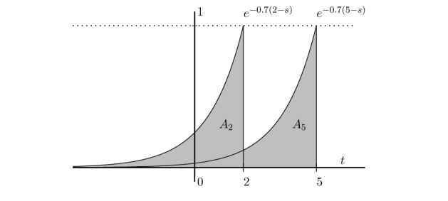
Figure 1: Example of a relevant choice of the trawl: $A_{t}=\{(x,s):s\leq t,0\leq x\leq\exp(-0.7(t-s))\}$. The shape of the trawl does not change as time $t$ progresses and, hence, we obtain a stationary process. The value of the process is obtained by evaluating $L(A_{t})$ for each $t$.

4.2 Cumulants and correlation structure

From Barndorff-Nielsen (2011) we know that the trawl process defined above is a strictly stationary stochastic process, and we can easily derive the cumulant transform of a trawl process, which is given by

$$C(\zeta\ddagger Y_{t}):=\mathbb{E}(\exp(i\zeta Y_{t}))=\mathit{L}eb(A)C(\zeta\ddagger L^{\prime}):=\mathit{L}eb(A)\mathbb{E}(\exp(i\zeta L^{\prime})).$$ (29)

From the equation (29), we see immediately that the law of the trawl process is infinitely divisible since the corresponding Lévy seed has infinitely divisible law.

Remark 7.

To any infinitely divisible law $\pi$ there exists a stationary trawl process having $\pi$ as its one-dimensional marginal law. This follows from formula (29), cf. Barndorff-Nielsen (2011)

We can now easily derive the cumulants of the trawl process which are given by $\kappa_{i}(Y_{t})=\mathit{L}eb(A)\kappa_{i}(L^{\prime})$, for $i\in{I\!\!N}$, provided they exist. In particular, the mean and variance are given by

$$\mathbb{E}(Y_{t})=\mathit{L}eb(A)\ \mathbb{E}(L^{\prime}), Var(Y_{t})=\mathit{L}eb(A)\ Var(L^{\prime}).$$

Marginally, we see that the precise shape of the trawl does not have any impact on the distribution of the process. The quantity which matters here is the size, i.e. the Lebesgue measure, of the trawl. So two different specifications of the ambit set, which have the same size, are not identified based on the marginal distribution only.

However, we will see that the shape of the trawl determines the autocorrelation function. More precisely, the autocorrelation structure is given as follows. Let $h>0$, then

$$\rho(h):=Cov(Y_{t},Y_{t+h})=\mathit{L}eb(A\cap A_{h})Var(L^{\prime}).$$ (30)

For the autocorrelation, we get

$$r(h)=Cor(Y_{t},Y_{t+h})=\frac{\mathit{L}eb(A\cap A_{h})}{\mathit{L}eb(A)}.$$

4.3 Lévy-Itô decomposition for trawl processes

In the following we study some of the sample path properties of trawl processes. First of all, we study a representation result for trawl process $Y$, where we split the process into a drift part, a Gaussian part and a jump part in a similar fashion as in the classical Lévy-Itô decomposition. Recall that $L$ is a homogeneous Lévy basis on $\mathbb{R}^{d}\times\mathbb{R}$. In the following, $s$ denotes the one dimensional temporal variable and ${\boldsymbol{\xi}}$ denotes the $d$-dimensional spatial variable.

From the Lévy-Itô decomposition, see (5), we get the following representation result for the trawl process $Y_{t}=L(A_{t})$ defined in (28), i.e.

$$\begin{split}L(A_{t})&=a\mathit{L}eb(A)+W(A_{t})+\int_{\{|x|>1\}}xN(dx,A_{t})+\int_{\{|x|\leq 1\}}x(N-n)(dx,A_{t})\\ &=a\mathit{L}eb(A)+W(A_{t})+\int_{A_{t}}\int_{\{|x|>1\}}xN(dx,d{\boldsymbol{\xi}},ds)+\int_{A_{t}}\int_{\{|x|\leq 1\}}x(N-n)(dx,d{\boldsymbol{\xi}},ds),\end{split}$$ (31)

where $W(A_{t})\sim N(0,b\mathit{L}eb(A))$ and $n(dx,d{\boldsymbol{\xi}},ds)=\nu(dx)d{\boldsymbol{\xi}}ds$ and $\mathit{L}eb(A_{t})=\mathit{L}eb(A)$.

Example 8.

Suppose the trawl process $Y_{t}$ is defined based on a Lévy basis with characteristic quadruplet $(0,b,0,\mathit{L}eb)$. Then it can be written as

$$Y_{t}=W(A_{t})\sim N(0,b\mathit{L}eb(A)).$$

Assume further that $d=1$ and that the trawl is given by $A_{t}=\{(x,s):s\leq t,0\leq x\leq\exp(-\lambda(t-s))\}$, for a positive constant $\lambda>0$. Then $\mathit{L}eb(A_{t})=\frac{1}{\lambda}$, hence $Y_{t}=W(A_{t})\sim N(0,\frac{b}{\lambda})$ and the autocorrelation function is given by $r(h)=\exp(-\lambda h)$, for $h\geq 0$.

4.4 Generalised cumulant functional

We have already studied the cumulant function of Lévy bases and ambit fields. Here, we will in addition focus on the more general cumulant functional of a trawl process, which sheds some light on important properties of trawl processes.

Definition 15.

Let $Y=(Y_{t})$ denote a stochastic process and let $\mu$ denote any non-random measure such that

$$\mu(Y)=\int_{\mathbb{R}}Y_{t}\,\mu(dt)<\infty,$$

where the integral should exist a.s.. The generalised cumulant functional of $Y$ w.r.t. $\mu$ is defined as

$$C\{\theta\ddagger\mu(Y)\}=\log\mathbb{E}\left(\exp\left(i\theta\mu(Y)\right)\right).$$

When we compute the cumulant functional for a trawl process, we obtain the following result.

Proposition 5.

Let $Y_{t}=L(A_{t})$ denote a trawl process and let $\mu$ denote any non-random measure such that $\mu(Y)=\int_{\mathbb{R}}Y_{t}\,\mu(dt)<\infty$, a. s.. Given the trawl $A$, we will further assume that for all ${\boldsymbol{\xi}}\in\mathbb{R}^{d}$,

$$h_{A}({\boldsymbol{\xi}},s)=\left(\int_{\mathbb{R}}1_{A}({\boldsymbol{\xi}},s-t)\mu(dt)\right)<\infty,$$

and that $h_{A}({\boldsymbol{\xi}},s)$ is integrable with respect to the Lévy basis $L$. Then the cumulant function of $\mu(Y)$ is given by

$$\begin{split}C\{\theta\ddagger\mu(Y)\}&=i\theta a\int_{\mathbb{R}\times\mathbb{R}^{d}}h_{A}({\boldsymbol{\xi}},s)d{\boldsymbol{\xi}}ds-\frac{1}{2}\theta^{2}b\int_{\mathbb{R}\times\mathbb{R}^{d}}h_{A}^{2}({\boldsymbol{\xi}},s)d{\boldsymbol{\xi}}ds\\ &\hskip 14.22636pt+\int_{\mathbb{R}\times\mathbb{R}^{d}}\int_{\mathbb{R}}\left(\exp(i\theta ux)-1-i\theta ux\mathbf{I}_{[-1,1]}(x)\right)\nu(dx)\chi(du),\end{split}$$ (32)

where $\chi$ is the measure on $\mathbb{R}$ obtained by lifting the Lebesgue measure on $\mathbb{R}^{d}\times\mathbb{R}$ to $\mathbb{R}$ by the mapping $\left({\boldsymbol{\xi}},s\right)\rightarrow({\boldsymbol{\xi}},h_{A}(s,{\boldsymbol{\xi}}))$.

Proof.

An application of Fubini’s theorem (see e.g. Barndorff-Nielsen & Basse-O’Connor (2011)) yields

$$\mu(Y) =\int_{\mathbb{R}}\int_{\mathbb{R}\times\mathbb{R}^{d}}1_{A}({\boldsymbol{\xi}},s-t)L(d{\boldsymbol{\xi}},ds)\,\mu(dt)=\int_{\mathbb{R}\times\mathbb{R}^{d}}\underbrace{\left(\int_{\mathbb{R}}1_{A}({\boldsymbol{\xi}},s-t)\mu(dt)\right)}_{=h_{A}({\boldsymbol{\xi}},s)}L(d{\boldsymbol{\xi}}^{,}ds)$$

$$=\int_{\mathbb{R}\times\mathbb{R}^{d}}h_{A}({\boldsymbol{\xi}},s)L(d{\boldsymbol{\xi}},ds).$$

From this we find that the cumulant function of $\mu(Y)$, i.e. the generalised cumulant functional of $Y$ w.r.t. $\mu$, is given by

$$C\{\theta\ddagger\mu(Y)\}=\int_{\mathbb{R}\times\mathbb{R}^{d}}C\{\theta h_{A}({\boldsymbol{\xi}},s)\ddagger L^{\prime}\}d{\boldsymbol{\xi}}ds$$

$$=i\theta a\int_{\mathbb{R}\times\mathbb{R}^{d}}h_{A}({\boldsymbol{\xi}},s)d{\boldsymbol{\xi}}ds-\frac{1}{2}\theta^{2}b\int_{\mathbb{R}\times\mathbb{R}^{d}}h_{A}^{2}({\boldsymbol{\xi}},s)d{\boldsymbol{\xi}}ds$$

$$\hskip 14.22636pt+\int_{\mathbb{R}\times\mathbb{R}^{d}}\int_{\mathbb{R}}\left(\exp(i\theta h_{A}({\boldsymbol{\xi}},s)x)-1-i\theta h_{A}({\boldsymbol{\xi}},s)x\mathbf{I}_{[-1,1]}(x)\right)\nu(dx)d{\boldsymbol{\xi}}ds.$$

Note that the latter part, i.e. the jump part of $C\{\theta\ddagger\mu(Y)\}$, can be recast as

$$\int_{\mathbb{R}\times\mathbb{R}^{d}}\int_{\mathbb{R}}\left(\exp(i\theta h_{A}({\boldsymbol{\xi}},s)x)-1-i\theta h_{A}({\boldsymbol{\xi}},s)x\mathbf{I}_{[-1,1]}(x)\right)\nu(dx)d{\boldsymbol{\xi}}ds$$

$$=\int_{\mathbb{R}\times\mathbb{R}^{d}}\int_{\mathbb{R}}\left(\exp(i\theta ux)-1-i\theta ux\mathbf{I}_{[-1,1]}(x)\right)\nu(dx)\chi(du),$$

where $\chi$ is the measure defined as above. Then the result follows. ∎

In the following, we mention three relevant choices of the measure $\mu$. Let $\delta_{t}$ denote the Dirac measure at $t$. We start with a very simple case:

Example 9.

Suppose $\mu(t)=\delta(dt)$ for a fixed $t$. Hence

$$h_{A}({\boldsymbol{\xi}},s)=\left(\int_{\mathbb{R}}1_{A}({\boldsymbol{\xi}},s-t)\mu(dt)\right)=1_{A}({\boldsymbol{\xi}},s-t)<\infty,$$

and clearly, $h_{A}({\boldsymbol{\xi}},s)$ is integrable with respect to $L$. Then

$$C\{\theta\ddagger\mu(Y)\}=C\{\theta\ddagger Y_{t}\}=\mathit{L}eb(A)C\{\theta\ddagger L^{\prime}\}.$$

This is exactly the result we derived in Section 4.2 above. More interesting is the case when $\mu$ is given by a linear combination of different Dirac measures, since this allows us to derive the joint finite dimensional laws of the trawl process and not just the distribution for fixed $t$.

Example 10.

Suppose $\mu\left(\mathrm{d}t\right)=\theta_{1}\delta_{t_{1}}\left(\mathrm{d}t\right)+\cdots+\theta_{n}\delta_{t_{n}}\left(\mathrm{d}t\right)$ for constants $\theta_{1},\dots,\theta_{n}\in\mathbb{R}$ and times $t_{1}<\cdots<t_{n}$ for $n\in{I\!\!N}$. As in the example before, the integrability conditions which were needed to derive (32) are satisfied and, hence, (32) gives us the cumulant function of the joint law of $Y_{t_{1}},\dots,Y_{t_{n}}$.

Finally, another case of interest is the integrated trawl process, which we study in the next example.

Example 11.

Let $\mu\left(\mathrm{d}t\right)=1_{I}\left(t\right)\mathrm{d}t$ for an interval $I$ of $\mathbb{R}$. Then (32) determines the law of $\int_{I}Y_{s}\mathrm{d}s$.

Remark 8.

The last example is particularly relevant if the trawl process is for instance used for modelling stochastic volatility. Note that such an application is feasible since the trawl process is stationary and we can formulate assumptions which would ensure the positivity of the process as well (e.g. if we work with a Lévy subordinator as the corresponding Lévy seed). In that context, integrated volatility is a quantity of key interest.

4.5 The increment process

Finally, we focus on the increments of a trawl process. Note that whatever the type of trawl, we have the following representation for the increments of the process for $s<t$,

$$Y_{t}-Y_{s}=L\left(A_{t}\backslash A_{s}\right)-L\left(A_{s}\backslash A_{t}\right),\qquad\text{almost surely}.$$ (33)

Due to the independence of $L\left(A_{t}\backslash A_{s}\right)$ and $-L\left(A_{s}\backslash A_{t}\right)$, we get the following representation for the cumulant function of the returns

$$\begin{split}C(\zeta\ddagger Y_{t}-Y_{s})&=C(\zeta\ddagger L\left(A_{t}\backslash A_{s}\right))+C(-\zeta\ddagger L\left(A_{s}\backslash A_{t}\right))\\ &=\mathit{L}eb(A_{t}\backslash A_{s})C(\zeta\ddagger L^{\prime})+\mathit{L}eb(A_{s}\backslash A_{t})C(-\zeta\ddagger L^{\prime})\\ &=\mathit{L}eb(A_{t-s}\backslash A_{0})C(\zeta\ddagger L^{\prime})+\mathit{L}eb(A_{0}\backslash A_{t-s})C(-\zeta\ddagger L^{\prime}).\end{split}$$ (34)

4.6 Applications of trawl processes

Trawl processes constitute a class of stationary infinitely divisible stochastic processes and can be used in various applications. E.g. we already pointed out above that they could be used for modelling stochastic volatility or intermittency. In a recent article by Barndorff-Nielsen, Lunde, Shephard & Veraart (2012), integer-valued trawl processes have been used to model count data or integer-valued data which are serially dependent. Speaking generally, trawl processes can be viewed as a flexible class of stochastic processes which can be used to model stationary time series data, where the marginal distribution and the autocorrelation structure can be modelled independently from each other.

5 Tempo-spatial stochastic volatility/intermittency

Stochastic volatility/intermittency plays a key role in various applications including turbulence and finance. While a variety of purely temporal stochastic volatility/intermittency models can be found in the literature, suitable tempo-spatial stochastic volatility/intermittency models still need to be developed.

Volatility modulation within the framework of an ambit field can be achieved by four complementary methods: By introducing a stochastic integrand (the term $\sigma_{t}({\bf x})$ in the definition of an ambit field), or by (extended) subordination or by probability mixing or Lévy mixing. We will discuss all four methods in the following.

5.1 Volatility modulation via a stochastic integrand

Stochastic volatility in form of a stochastic integrand has already been included in the initial definition of an ambit field, see (16). The interesting aspect, which we have not addressed yet, is how a model for the stochastic volatility field $\sigma_{t}(x)$ can be specified in practice. We will discuss several relevant choices in more detail in the following.

There are essentially two approaches which can be used for constructing a relevant stochastic volatility field: Either one specifies the stochastic volatility field directly as a random field (e.g. as another ambit field), or one starts from a purely temporal (or spatial) stochastic volatility process and then generalises the stochastic process to a random field in a suitable way. In the following, we will present examples of both types of construction.

5.1.1 Kernel-smoothing of a Lévy basis

First, we focus on the modelling approach where we directly specify a random field for the volatility field. A natural starting point for modelling the volatility is given by kernel-smoothing of a homogeneous Lévy basis – possibly combined with a (nonlinear) transformation to ensure positivity. For instance, let

$$\sigma^{2}_{t}({\bf x})=V\left(\int_{\mathbb{R}_{t}\times\mathbb{R}^{d}}j({\bf x},{\boldsymbol{\xi}},t-s)L^{\sigma}(d{\boldsymbol{\xi}},ds)\right),$$ (35)

where $L^{\sigma}$ is a homogeneous Lévy basis independent of $L$, $j:\mathbb{R}^{d+1+d}\mapsto\mathbb{R}_{+}$ is an integrable kernel function satisfying $j({\bf x},u,{\boldsymbol{\xi}})=0$ for $u<0$ and $V:\mathbb{R}\to\mathbb{R}_{+}$ is a continuous, non-negative function. Note that $\sigma^{2}$ defined by (35) is stationary in the temporal dimension. As soon as $j({\bf x},{\boldsymbol{\xi}},t-s)=j^{*}({\bf x}-{\boldsymbol{\xi}},t-s)$ for some function $j^{*}$ in (35), then the stochastic volatility is both stationary in time and homogeneous in space.

Clearly, the kernel function $j$ determines the tempo-spatial autocorrelation structure of the volatility field.

Let us discuss some examples next.

Example 12 (Tempo-spatial trawl processes).

Suppose the kernel function is given by

$$j({\bf x},{\boldsymbol{\xi}},t-s)={\bf I}_{A^{\sigma}}({\boldsymbol{\xi}}-{\bf x},s-t),$$

where $A^{\sigma}\subset\mathbb{R}^{d}\times(-\infty,0]$. Further, let $A_{t}^{\sigma}({\bf x})=A^{\sigma}+({\bf x},t)$; hence $A_{t}^{\sigma}({\bf x})$ is a homogeneous and nonanticipative ambit set. Then

$$\sigma_{t}^{2}({\bf x})=V\left(\int_{\mathbb{R}_{t}\times\mathbb{R}^{d}}{\bf I}_{A}^{\sigma}({\boldsymbol{\xi}}-{\bf x},s-t)L^{\sigma}(d{\boldsymbol{\xi}},ds)\right)=V\left(\int_{A_{t}^{\sigma}({\bf x})}L^{\sigma}(d{\boldsymbol{\xi}},ds)\right)=V\left(L^{\sigma}(A^{\sigma}_{t}({\bf x}))\right).$$

Note that the random field $L^{\sigma}(A^{\sigma}_{t}({\bf x}))$ can be regarded as a tempo-spatial trawl process.

Example 13.

Let

$$j({\bf x},{\boldsymbol{\xi}},t-s)=j^{*}({\bf x},{\boldsymbol{\xi}},t-s){\bf I}_{A^{\sigma}({\bf x})}({\boldsymbol{\xi}},s-t),$$

for an integrable kernel function $j^{*}$ and where $A^{\sigma}({\bf x})\subset\mathbb{R}^{d}\times(-\infty,0]$. Further, let $A_{t}^{\sigma}({\bf x})=A^{\sigma}({\bf x})+({\bf 0},t)$. Then

$$\sigma^{2}_{t}({\bf x})=V\left(\int_{A_{t}^{\sigma}({\bf x})}j({\boldsymbol{\xi}},{\bf x},t-s)L^{\sigma}(d{\boldsymbol{\xi}},ds)\right),$$ (36)

which is a transformation of an ambit field (without stochastic volatility).

Let us look at some more concrete examples for the stochastic volatility field.

Example 14.

A rather simple specification is given by choosing $L^{\sigma}$ to be a standard normal Lévy basis and $V(x)=x^{2}$. Then $\sigma_{s}^{2}({\boldsymbol{\xi}})$ would be positive and pointwise $\chi^{2}$-distributed with one degree of freedom.

Example 15.

One could also work with a general Lévy basis, in particular Gaussian, and $V$ given by the exponential function, see e.g. Barndorff-Nielsen & Schmiegel (2004) and Schmiegel et al. (2005).

Example 16.

A non-Gaussian example would be to choose $L^{\sigma}$ as an inverse Gaussian Lévy basis and $V$ to be the identity function.

Example 17.

We have already mentioned that the kernel function $j$ determines the autocorrelation structure of the volatility field. E.g. in the absence of spatial correlation one could start off with the choice $j({\bf x},t-s,{\boldsymbol{\xi}})=\exp(-\lambda(t-s))$ for $\lambda>0$ mimicking the Ornstein-Uhlenbeck-based stochastic volatility models, see e.g. Barndorff-Nielsen & Schmiegel (2004).

5.1.2 Ornstein-Uhlenbeck volatility fields

Next, we show how to construct a stochastic volatility field by extending a stochastic process by a spatial dimension. Note that our objective is to construct a stochastic volatility field which is stationary (at least in the temporal direction). Clearly, there are many possibilities on how this can be done and we focus on a particularly relevant one in the following, namely the Ornstein-Uhlenbeck-type volatility field (OUTVF). The choice of using an OU process as the stationary base component is motivated by the fact that non-Gaussian OU-based stochastic volatility models, as e.g. studied in Barndorff-Nielsen & Shephard (2001), are analytically tractable and tend to perform well in practice, at least in the purely temporal case. In the following, we will restrict our attention to the case $d=1$, i.e. that the spatial dimension is one-dimensional.

Suppose now that $\tilde{Y}$ is a positive OU type process with rate parameter $\lambda>0$ and generated by a Lévy subordinator $Y$, i.e.

$$\tilde{Y}_{t}=\int_{-\infty}^{t}e^{-\lambda\left(t-s\right)}\mathrm{d}Y_{s},$$

We call a stochastic volatility field $\sigma_{t}^{2}\left(x\right)$ on $\mathbb{R}\times\mathbb{R}$ an Ornstein-Uhlenbeck-type volatility field (OUTVF), if it is defined as follows

$$\tau_{t}\left(x\right)=\sigma_{t}^{2}\left(x\right)=e^{-\mu x}\tilde{Y}_{t}+\int_{0}^{x}e^{-\mu\left(x-\xi\right)}\mathrm{d}Z_{\xi|t},$$ (37)

where $\mu>0$ is the spatial rate parameter and where $\mathcal{Z}=\left\{Z_{\cdot|t}\right\}_{t\in\mathbb{R}_{+}}$ is a family of Lévy processes, which we define more precisely in the next but one paragraph.

Note that in the above construction, we start from an OU process in time. In particular, $\tau_{t}(0)$ is an OU process. The spatial structure is then introduced by two components: First, we we add an exponential weight $e^{-\mu x}$ in the spatial direction, which reaches its maximum for $x=0$ and decays the further away we get from the purely temporal case. Second, an integral is added which resembles an OU-type process in the spatial variable $x$. However, note here that the integration starts from $0$ rather than from $-\infty$, and hence the resulting component is not stationary in the spatial variable $x$. (This could be changed if required in a particular application.)

Let us now focus in more detail on how to define the family of Lévy processes $\mathcal{Z}$. Suppose $\tilde{X}=\left\{\tilde{X}_{t}\right\}_{t\in\mathbb{R}}$ is a stationary, positive and infinitely divisible process on $\mathbb{R}$. Next we define $Z_{|\cdot}=\left\{Z_{x|\cdot}\right\}_{x\in\mathbb{R}_{+}}$ as the so-called Lévy supra-process generated by $\tilde{X}$, that is $\left\{Z_{x|\cdot}\right\}_{x\in\mathbb{R}_{+}}$ is a family of stationary processes such that $Z_{|\cdot}$ has independent increments, i.e. for any $0<x_{1}<x_{2}<\cdots<x_{n}$ the processes $Z_{x_{1}|\cdot},Z_{x_{2}|\cdot}-Z_{x_{1}|\cdot},\dots,Z_{x_{n}|\cdot}-Z_{x_{n-1|\cdot}}$ are mutually independent, and such that for each $x$ the cumulant functional of $Z_{x|\cdot}$ equals $x$ times the cumulant functional of $\tilde{X}$, i.e.

$$\mathrm{C}\{m\ddagger Z_{x|\cdot}\}=x\mathrm{C}\{m\ddagger\tilde{X}\},$$

where

$$\mathrm{C}\{m\ddagger\tilde{X}\}=\log\mathrm{E}\left\{e^{im\left(\tilde{X}\right)}\right\},$$

with $m\left(\tilde{X}\right)=\int\tilde{X}_{s}m\left(\mathrm{d}s\right)$, $m$ denoting an ‘arbitrary’ signed measure on $\mathbb{R}$. Then at any $t\in\mathbb{R}$ the values $Z_{x|t}$ of $Z_{\cdot|\cdot}$ at time $t$ as $x$ runs through $\mathbb{R}_{+}$ constitute a Lévy process that we denote by $Z_{\cdot|t}$. This is the Lévy process occurring in the integral in (37).

Note that $\tau$ is stationary in $t$ and that $\tau_{t}\left(x\right)\rightarrow\tilde{Y}_{t}$ as $x\rightarrow 0$.

Example 18.

Now suppose, for simplicity, that $\tilde{X}$ is an OU process with rate parameter $\kappa$ and generated by a Lévy process $X$. Then

$$\mathrm{Cov}\{\tau_{t}\left(x\right),\tau_{t^{\prime}}\left(x^{\prime}\right)\}=\frac{1}{2}\left(\mathrm{Var}\{Y_{1}\}\lambda^{-1}e^{-\lambda\left(\left|t-t^{\prime}\right|\right)-\mu\left(x+x^{\prime}\right)}+\mathrm{Var}\{\tilde{X}_{0}\}\mu^{-1}e^{-\kappa|t-t^{\prime}|-\mu\left|x-x^{\prime}\right|}\right.$$

$$\left.-\mathrm{Var}\{\tilde{X}_{0}\}\mu^{-1}e^{-\kappa\left|t-t^{\prime}\right|-\mu\left(x+x^{\prime}\right)}\right).$$

If, furthermore, $\mathrm{Var}\{Y_{1}\}=\mathrm{Var}\{\tilde{X}_{0}\}$ and $\kappa=\lambda=\mu$ then for fixed $x$ and $x^{\prime}$ the autocorrelation function of $\tau$ is

$$\mathrm{Cor}\{\tau_{t}\left(x\right),\tau_{t^{\prime}}\left(x^{\prime}\right)\}=e^{-\kappa|t-t^{\prime}|}e^{-\kappa\left|x-x^{\prime}\right|}.$$

This type of construction can of course be generalised in a variety of ways, including dependence between $X$ and $Y$ and also superposition of OU processes.

Note that the process $\tau_{t}(x)$ is in general not predictable, which is disadvantageous given that we want to construct Walsh-type stochastic integrals. However, if we choose $\widetilde{X}$ to be of OU type, then we obtain a predictable stochastic volatility process.

5.2 Extended subordination and meta-times

An alternative way of volatility modulation is by means of (extended) subordination. Extended subordination and meta-times are important concepts in the ambit framework, which have recently been introduced by Barndorff-Nielsen (2010) and Barndorff-Nielsen & Pedersen (2012), and we will review their main results in the following. Note that extended subordination generalises the classical concept of subordination of Lévy processes to subordination of Lévy bases. This in turn will be based on a concept of meta-times.

5.2.1 Meta-times

This section reviews the concept of meta-times, which we will link to the idea of extended subordination in the following section.

Definition 16.

Let $S$ be a Borel set in $\mathbb{R}^{k}$. A meta-time $\mathbf{T}$ on $S$ is a mapping from $\mathcal{B}_{b}(S)$ into $\mathcal{B}_{b}(S)$ such that

1. $\mathbf{T}\left(A\right)$ and $\mathbf{T}\left(B\right)$ are disjoint whenever $A,B\in\mathcal{B}_{b}(S)$ are disjoint.

2. $\mathbf{T}\left(\cup_{j=1}^{\infty}A_{j}\right)=\cup_{j=1}^{\infty}\mathbf{T}\left(A_{j}\right)$ whenever $A_{1},A_{2},\dots\in\mathcal{B}_{b}(S)$ are disjoint and $\cup_{j=1}^{\infty}A_{j}\in\mathcal{B}_{b}(S)$.

A slightly more general definition is the following one.

Definition 17.

Let $S$ be a Borel set in $\mathbb{R}^{k}$. A full meta-time $\mathbf{T}$ on $S$ is a mapping from $\mathcal{B}(S)$ into $\mathcal{B}(S)$ such that

1. $\mathbf{T}\left(A\right)$ and $\mathbf{T}\left(B\right)$ are disjoint whenever $A,B\in\mathcal{B}(S)$ are disjoint.

2. $\mathbf{T}\left(\cup_{j=1}^{\infty}A_{j}\right)=\cup_{j=1}^{\infty}\mathbf{T}\left(A_{j}\right)$ whenever $A_{1},A_{2},\dots\in\mathcal{B}(S)$ are disjoint.

Suppose $\mu$ is a measure on $\left(S,\mathcal{B}(S)\right)$ and let $\mathbf{T}$ be a full meta-time on $S$. Define $\mu\left(\cdot\curlywedge\mathbf{T}\right)$ as the mapping from  $\mathcal{B}(S)$ into $\mathbb{R}$ given by $\mu\left(A\curlywedge\mathbf{T}\right)=\mu\left(\mathbf{T}\left(A\right)\right)$ for any $A\in\mathcal{B}(S)$. Then $\mu\left(\cdot\curlywedge\mathbf{T}\right)$ is a measure on $\left(S,\mathcal{B}(S)\right)$. We speak of $\mu\left(\cdot\curlywedge\mathbf{T}\right)$ as the subordination of $\mu$ by $\mathbf{T}$. Similarly, if $\mathbf{T}$ is a meta-time on $S$ we speak of $\mu\left(A\curlywedge\mathbf{T}\right)=\mu\left(\mathbf{T}\left(A\right)\right)$ for $A\in\mathcal{B}_{b}(S)$ as the subordination of $\mu$ by $\mathbf{T}$.

Let us now recall an important result, which says that any measure, which is finite on compacts, can be represented as the image measure of the Lebesgue measure of a meta-time.

Lemma 2.

Barndorff-Nielsen & Pedersen (2012, Lemma 3.1) Let $T$ be a measure on $\mathcal{B}(S)$ satisfying $T\left(A\right)<\infty$ for all $A\in\mathcal{B}_{b}(S)$  Then there exists a meta-time $\mathbf{T}$ such that, for all $A\in\mathcal{B}_{b}(S)$, we have

$$T\left(A\right)=\mathrm{Leb}\left(\mathbf{T}\left(A\right)\right).$$

We speak of $\mathbf{T}$ as a meta-time associated to $T$.

Remark 9.

$\mathbf{T}$ can be chosen so that $\mathbf{T}\left(A\right)=\left\{\mathbb{T}\left({\bf x}\right):{\bf x}\in A\right\}$ where $\mathbb{T}$ is the inverse of a measurable mapping $\mathbb{U}:S\rightarrow S$ determined from $\mathbf{T}$. Here integration under subordination satisfies

$$\int_{S}f\left(s\right)\mu\left(\mathrm{d}s\curlywedge\mathbf{T}\right)=\int_{S}f\left(s\right)\mu\left(\mathbf{T}\left(\mathrm{d}s\right)\right)=\int_{S}f\left(\mathbb{U}\left(u\right)\right)\mu\left(\mathrm{d}u\right).$$

Suppose $S$ is open and that $T$ is a measure on $S$ which is absolutely continuous with density $\tau$. If we can find a mapping $\mathbb{T}$ from $S$ to $S$ sending Borel sets into Borel sets and such that the Jacobian of $\mathbb{T}$ exists and satisfies

$$|\mathbb{T}_{/{\bf x}}|=\tau\left({\bf x}\right),$$

then $\mathbf{T}$ given by $\mathbf{T}\left(A\right)=\left\{\mathbb{T}\left({\bf x}\right):{\bf x}\in A\right\}$, is a natural choice of meta-time induced by $T$. In fact, by the change of variable formula,

$$\mathit{L}eb\left(\mathbf{T}\left(A\right)\right)=\int 1_{\mathbf{T}\left(A\right)}(y)\mathrm{d}y=\int 1_{A}\left({\bf x}\right)|\mathbb{T}_{/{\bf x}}|\mathrm{d}{\bf x}=\int_{A}\tau\left({\bf x}\right)\mathrm{d}{\bf x}=T\left(A\right),$$

verifying that $\mathbf{T}$ is a meta-time associated to $T$.

Remark 10.

$\mathbf{T}$ is not uniquely determined by $T$ and two different meta-times associated to $T$ may yield different subordinations of one and the same measure $\mu$.

5.2.2 Extended subordination of Levy bases

Let us now study the concept of subordination in the case where we deal with a Lévy basis. Let $T$ be a full random measure on $S$. Then, by Lemma 2, there exists a.s. a random meta-time $\mathbf{T}$ determined by $T$ and with the property that $\mathit{L}eb\left(\mathbf{T}\left(A\right)\right)=T\left(A\right)$, for all $A\in\mathcal{B}_{b}(S)$. There are two cases of particular interest to us. First, $\mathbf{T}$ is induced by a Lévy basis $L$ on $S$ that is non-negative, dispersive and of finite variation. Second, $\mathbf{T}$ is induced by an absolutely continuous random measure $T$ on $S$ with a non-negative density $\tau$ satisfying $T\left(A\right)=\int_{A}\tau\left({\bf z}\right)\mathrm{d}{\bf z}<\infty$ for all $A\in\mathcal{B}_{b}(S)$.

Definition 18.

Let $L$ be a Lévy basis on $S$ and let $T$, independent of $L$, be a full random measure on $S$. The extended subordination of $L$ by $T$ is the random measure $L(\cdot\curlywedge T)$ defined by

$$L(A\curlywedge T)=L\left(\mathbf{T}\left(A\right)\right)$$

for all $A\in\mathcal{B}_{b}\left(S\right)$ and where $\mathbf{T}$ is a meta-time induced by $T$ (in which case $\mathit{L}eb\left(\mathbf{T}\left(A\right)\right)=T\left(A\right)$).

Note that the Lévy basis $L$ may be $n$-dimensional. We shall occasionally write $L\curlywedge T$ for $L\left(\cdot\curlywedge T\right)$, which is a random measure on $(S,\mathcal{B}_{b}(S))$.

In the case that $L$ is a homogeneous Lévy basis and since $T$ is assumed to be independent of $L$, $L(\cdot\curlywedge T)$ is a (in general not homogeneous) Lévy basis, whose conditional cumulant function satisfies

$$\mathrm{C}\{\zeta\ddagger L(A\curlywedge T)|T\}=T(A)\mathrm{C}\{\zeta\ddagger L^{\prime}\}$$ (38)

for all $A\in\mathcal{B}_{b}(\mathcal{S})$ and where $L^{\prime}$ is the Lévy seed of $L$. On a distributional level one may, without attention to the full probabilistic definition of $L(\cdot\curlywedge T)$ presented above, carry out many calculations purely from using the identity established in (38).

Remarks

The two key formulae $L(\cdot\curlywedge T)=L\left(\mathbf{T}\left(\cdot\right)\right)$ and $\mathit{L}eb\left(\mathbf{T}\left(A\right)\right)=T\left(A\right)$ show that the concepts of extended subordination and meta-time together generalise the classical subordination of Lévy processes. Provided that $L$ is homogeneous we have that

$$\mathrm{C}\{\zeta\ddagger L(A\curlywedge T)|T\}=\mathit{L}eb\left(\mathbf{T}\left(A\right)\right)\mathrm{C}\{\zeta\ddagger L^{\prime}\},$$

and hence

$$\mathrm{C}\{\zeta\ddagger L(A\curlywedge T)\}=\log\mathrm{E}\left\{e^{T\left(A\right)\mathrm{C}\{\zeta\ddagger L^{\prime}\}}\right\}.$$

Hence we can deduce the following results.

• The values of the subordination $L(\cdot\curlywedge T)$ of $L$ are infinitely divisible provided the values of $T$ are infinitely divisible and $L$ is homogeneous.

• If $L$ is homogeneous and if $T$ is a homogeneous Lévy basis then $L(\cdot\curlywedge T)$ is a homogeneous Lévy basis.

• In general, $\mathbf{T}$ is not uniquely determined by $T$. Nevertheless, provided the Lévy basis $L$ is homogeneous the law of $L(\cdot\curlywedge T)$ does not depend on the choice of meta-time $\mathbf{T}$.

Lévy-Itô type representation of $L\left(\cdot\curlywedge\cdot\right)$

We have already reviewed the Lévy-Itô representation for a dispersive Lévy basis $L$, see (5). It follows directly that the subordination of $L$ by the random measure $T$ with associated meta-time $\mathbf{T}$ has a Lévy-Itô type representation

$$L\left(A\curlywedge T\right) =a\left(\mathbf{T}\left(A\right)\right)+\sqrt{b(\mathbf{T}\left(A\right))}W\left(\mathbf{T}\left(A\right)\right)$$

$$+\int_{\{\left|y\right|>1\}}yN\left(dy;\mathbf{T}\left(A\right)\right)+\int_{\{\left|y\right|\leq 1\}}y\left(N-\nu\right)\left(dy;\mathbf{T}\left(A\right)\right).$$

Lévy measure of $L\curlywedge T$

Suppose for simplicity that $L\curlywedge T$ is non-negative. According to Barndorff-Nielsen (2010), the Lévy measure $\widetilde{\nu}$ of $L\curlywedge T$ is related to the Lévy measure $\nu$ of $T$ by

$$\widetilde{\nu}\left(\mathrm{d}x;s\right)=\int_{\mathbb{R}}P\left(L^{\prime}_{y}(s)\in dx\right)\nu\left(dy;s\right).$$

5.2.3 Extended subordination and volatility

In the context of ambit stochastics one considers volatility fields $\sigma$ in space-time, typically specified by the squared field $\tau_{t}\left({\bf x}\right)=\sigma_{t}^{2}\left({\bf x}\right)$. So far, we have used a stochastic volatility random field $\sigma$ in the integrand of the ambit field to introduce volatility modulation.

A complementary method consists of introducing stochastic volatility by extended subordination. The volatility is incorporated in the modelling through a meta-time associated to the measure $T$ on $S$ and given by

$$T\left(A\right)=\int_{A}\tau_{t}\left({\bf x}\right)\mathrm{d}{\bf x}\mathrm{d}t$$

A natural choice of meta-time is $\mathbf{T}\left(A\right)=\left\{\mathbb{T}\left({\bf x},t\right):\left({\bf x},t\right)\in A\right\}$, where $\mathbb{T}$ is the mapping given by

$$\mathbb{T}\left({\bf x},t\right)=\left({\bf x},\tau_{s}^{+}\left({\bf x}\right)\right)$$

and where

$$\tau_{t}^{+}\left({\bf x}\right)=\int_{0}^{t}\tau_{s}\left({\bf x}\right)\mathrm{d}s.$$

The above construction of a meta-time in a tempo-spatial model is very general. One can construct a variety of models for the random field $\tau_{t}({\bf x})$, which lead to new model specifications. Essentially, this leads us back to the problem we tackled in the previous Subsection, where we discussed how such fields can be modelled. For instance, one could model $\tau_{t}({\bf x})$ by an Ornstein-Uhlenbeck type volatility field or any other model discussed in Subsection 5.1. Clearly, the concrete choice of the model needs to be tailored to the particular application one has in mind.

5.3 Probability mixing and Lévy mixing

Volatility modulation can also be obtained through probability mixing as well as Lévy mixing.

The main idea behind the concept of probability or distributional mixing is to construct new distributions by randomising a parameter from a given parametric distribution.

Example 19.

Consider our very first base model (1). Now suppose that the corresponding Lévy basis is homogeneous and Gaussian, i.e. the corresponding Lévy seed is given by $L^{\prime}\sim N(\mu+\beta\sigma^{2},\sigma^{2})$ with $\mu,\beta\in\mathbb{R}$ and $\sigma^{2}>0$. Now we use probability mixing and suppose that in fact $\sigma^{2}$ is random. Hence, the conditional law of the Lévy seed is given by $L^{\prime}|\sigma\sim N(\mu+\beta\sigma^{2},\sigma^{2})$. Due to the scaling property of the Gaussian distribution, such a model can be represented as (16) and, hence, in this particular case probability mixing and stochastic volatility via a stationary stochastic integrand essentially have the same effect. Suppose that the conditional variance $\sigma^{2}$ has a generalised inverse Gaussian (GIG) distribution rather than being just a constant, then $L^{\prime}$ follows in fact a generalised hyperbolic (GH) distribution. Such a construction falls into the class of normal variance-mean mixtures.

In this context it is important to note that probability/distributional mixing does not generally lead to infinitely divisible distributions, see e.g. Steutel & van Harn (2004, Chapter VI). Hence Barndorff-Nielsen, Perez-Abreu & Thorbjørnsen (2012) propose to work with Lévy mixing instead of probability/distributional mixing. Lévy mixing is a method which (under mild conditions) leads to classes of infinitely divisible distributions again. Let us review the main idea behind that concept.

Let $L$ denote a factorisable Lévy basis on $\mathbb{R}^{k}$ with CQ $(a,b,\nu(dx),c)$. Suppose that the Lévy measure $\nu(dx)$ depends on a possibly multivariate parameter ${\boldsymbol{\theta}}\in\Theta$, say, where $\Theta$ denotes the parameter space. In that case, we write $\nu(dx;{\boldsymbol{\theta}})$. Then, the generalised Lévy measure of $L$ is given by $\nu(dx;{\boldsymbol{\theta}})c(d{\bf z})$. Now let $\gamma$ denote a measure on $\Theta$ and define

$$\tilde{n}(dx,d{\bf z})=\int_{\Theta}\nu(dx;{\boldsymbol{\theta}})\gamma(d{\boldsymbol{\theta}})c(d{\bf z}),$$

where we assume that

$$\int_{\mathbb{R}}(1\wedge x^{2})\tilde{n}(dx,d{\bf z})<\infty.$$ (39)

Then there exists a Lévy basis $\tilde{L}$ which has $\tilde{n}$ as its generalised Lévy measure. We call the Lévy basis $\tilde{L}$ the Lévy basis obtained by Lévy-mixing $L$ with the measure $\gamma$.

Let us study a concrete example of Lévy mixing in the following.

Example 20.

Suppose $L$ is a homogeneous Lévy basis with CQ given by $(0,0,\nu(dx),\mathit{L}eb)$ with $\nu(dx)=\theta\delta_{1}(dx)$ for $\theta>0$. I.e. the corresponding Lévy seed is given by $L^{\prime}\sim Poi(\theta)$. Now we do a Lévy-mixing of the intensity parameter $\theta$. Let

$$\tilde{n}(dx,d{\bf z})=\int_{\Theta}\theta\gamma(d\theta)\delta_{1}(dx)d{\bf z},$$

for a measure $\gamma$ satisfying condition (39). Let $\tilde{L}$ be the Lévy basis with CQ $(0,0,\int_{\Theta}\theta\gamma(dv)\delta_{1}(dx),\mathit{L}eb)$. In that case, the base model (1) would be transferred into a model of the form

$$\int_{\Theta}\int_{A_{t}({\bf x})}h({\bf x},t;{\boldsymbol{\xi}},s)\tilde{L}(d{\boldsymbol{\xi}},ds,dv).$$

Example 21.

Let us consider the example of a (sup)OU process, see Barndorff-Nielsen (2000), Barndorff-Nielsen & Stelzer (2011) and Barndorff-Nielsen, Perez-Abreu & Thorbjørnsen (2012). Let $L$ denote a subordinator with Lévy measure $\nu_{L}$ (and without drift) and consider an OU process

$$Y_{t}=\int_{-\infty}^{t}e^{-\theta(t-s)}dL(s),\qquad\theta>0.$$

A straightforward computation leads to the following expression for its cumulant function (for $\zeta\in\mathbb{R}$):

$$C\{\zeta\ddagger Y_{t}\}=\int_{0}^{\infty}\left(e^{i\zeta x}-1\right)\nu(dx;\theta),\quad\text{ where }\quad\nu(dx,\theta)=\int_{0}^{\infty}\nu_{L}(e^{\theta u}dx)du$$

is a mixture of $\nu_{L}$ with the Lebesgue measure. A Lévy mixing can be carried out with respect to the parameter $\theta$, i.e.

$$\tilde{\nu}(dx)=\int_{0}^{\infty}\nu(dx,\theta)\gamma(d\theta),$$

where $\gamma$ is a measure on $[0,\infty)$ satisfying $\int_{0}^{\infty}x\tilde{\nu}(dx)<\infty$. Then $\tilde{\nu}$ is a Lévy measure again. Now, let $\tilde{L}$ be the Lévy basis with extended Lévy measure

$$\nu_{L}(dx)du\gamma(d\theta),$$

and define the supOU process $\tilde{Y}_{t}$ w.r.t. $\tilde{L}$ by

$$\tilde{Y}_{t}=\int_{0}^{\infty}\int_{-\infty}^{t}e^{-\lambda(t-s)}\tilde{L}(ds,d\lambda).$$

Then the cumulant function of $\tilde{Y}_{t}$ is given by

$$C\{\zeta\ddagger\tilde{Y}_{t}\} =\int_{0}^{\infty}\int_{-\infty}^{t}C\{\zeta e^{-\theta(t-s)}\ddagger L_{1}\}ds\gamma(d\theta)=\int_{0}^{\infty}\int_{0}^{\infty}\left(e^{i\zeta e^{-\theta u}}-1\right)\nu_{L}(dx)du\gamma(d\theta)$$

$$=\int_{0}^{\infty}\left(e^{i\zeta x}-1\right)\tilde{\nu}(dx).$$

Hence, we have seen that a supOU process can be obtained from an OU process through Lévy-mixing.

5.4 Outlook on volatility estimation

Once a model is formulated and data are available the question of assessment of volatility arises and while we do not discuss this in any detail, tools for this are available for some special classes of ambit processes, see Barndorff-Nielsen et al. (2009); Barndorff-Nielsen, Corcuera & Podolskij (2011, 2012) and also Barndorff-Nielsen & Graversen (2011). Extending these results to general ambit fields and processes is an interesting direction for future research.

6 Conclusion and outlook

In this paper, we have given an overview of some of the main findings in ambit stochastics up to date, including a suitable stochastic integration theory, and have established new results on general properties of ambit field. The new results include sufficient conditions which ensure the smoothness of ambit fields. Also, we have formulated sufficient conditions which guarantee that an ambit field is a semimartingale in the temporal domain. Moreover, the concept of tempo-spatial stochastic volatility/intermittency within ambit fields has been further developed. Here our focus has been on four methods for volatility modulation: Stochastic scaling, stochastic time change and extended subordination of random measures, and probability and Lévy mixing of the volatility/intensity parameter.

Future research will focus on applications of the general classes of models developed in this paper in various fields, including empirical research on turbulence modelling as well as modelling e.g. the term structure of interest rates in finance by ambit fields. In this context, it will be important to establish a suitable estimation theory for general ambit fields as well as inference techniques.

References

- (1)
- Adler (1981) Adler, R. J. (1981), The geometry of random fields, John Wiley & Sons Ltd., Chichester. Wiley Series in Probability and Mathematical Statistics.
- Adler & Taylor (2007) Adler, R. J. & Taylor, J. E. (2007), Random fields and geometry, Springer Monographs in Mathematics, Springer, New York.
- Amiri (2009) Amiri, E. (2009), Bayesian modelling volatility of growth rate in atmospheric carbon dioxide concentrations, in ‘Proceedings of the 2009 Second International Conference on Environmental and Computer Science’, ICECS ’09, IEEE Computer Society, Washington, DC, USA, pp. 86–90.
- Azaïs & Wschebor (2009) Azaïs, J.-M. & Wschebor, M. (2009), Level sets and extrema of random processes and fields, John Wiley & Sons Inc., Hoboken, NJ.
- Barndorff-Nielsen (2000) Barndorff-Nielsen, O. E. (2000), ‘Superposition of Ornstein-Uhlenbeck type processes’, Rossiĭskaya Akademiya Nauk. Teoriya Veroyatnosteĭ i ee Primeneniya 45(2), 289–311.
- Barndorff-Nielsen (2010) Barndorff-Nielsen, O. E. (2010), Lévy bases and extended subordination. Thiele Centre Research Report No. 12, Aarhus University.
- Barndorff-Nielsen (2011) Barndorff-Nielsen, O. E. (2011), ‘Stationary infinitely divisible processes’, Brazilian Journal of Probability and Statistics 25, 294–322.
- Barndorff-Nielsen & Basse-O’Connor (2011) Barndorff-Nielsen, O. E. & Basse-O’Connor, A. (2011), ‘Quasi Ornstein-Uhlenbeck Processes’, Bernoulli 17(3), 916–941.
- Barndorff-Nielsen, Benth, Pedersen & Veraart (2012) Barndorff-Nielsen, O. E., Benth, F. E., Pedersen, J. & Veraart, A. E. D. (2012), On stochastic integration for volatility modulated Lévy-driven Volterra processes. Preprint available at http://arxiv.org/abs/1205.3275v1.
- Barndorff-Nielsen et al. (2010) Barndorff-Nielsen, O. E., Benth, F. E. & Veraart, A. E. D. (2010), Modelling electricity forward markets by ambit fields. Preprint.
- Barndorff-Nielsen, Benth & Veraart (2011) Barndorff-Nielsen, O. E., Benth, F. E. & Veraart, A. E. D. (2011), Ambit processes and stochastic partial differential equations, in G. Di Nunno & B. Øksendal, eds, ‘Advanced Mathematical Methods for Finance’, Springer, pp. 35–74.
- Barndorff-Nielsen, Benth & Veraart (2012) Barndorff-Nielsen, O. E., Benth, F. E. & Veraart, A. E. D. (2012), ‘Modelling energy spot prices by volatility modulated Lévy-driven Volterra processes’, Bernoulli . To appear.
- Barndorff-Nielsen et al. (2009) Barndorff-Nielsen, O. E., Corcuera, J. & Podolskij, M. (2009), ‘Power variation for Gaussian processes with stationary increments’, Stochastic Processes and Their Applications 119, 1845–1865.
- Barndorff-Nielsen, Corcuera & Podolskij (2011) Barndorff-Nielsen, O. E., Corcuera, J. & Podolskij, M. (2011), ‘Multipower variation for Brownian semistationary processes’, Bernoulli 17(4), 1159–1194.
- Barndorff-Nielsen, Corcuera & Podolskij (2012) Barndorff-Nielsen, O. E., Corcuera, J. & Podolskij, M. (2012), Limit theorems for functionals of higher order differences of Brownian semistationary processes, in A. E. Shiryaev, S. R. S. Vayadhan & E. Presman, eds, ‘Prokhorov and Contemporary Probability’. To appear.
- Barndorff-Nielsen & Graversen (2011) Barndorff-Nielsen, O. E. & Graversen, S. E. (2011), ‘Volatility determination in an ambit process setting’, Journal of Applied Probability 48A, 263–275. New frontiers in applied probability: a Festschrift for Søren Asmussen.
- Barndorff-Nielsen, Lunde, Shephard & Veraart (2012) Barndorff-Nielsen, O. E., Lunde, A., Shephard, N. & Veraart, A. E. D. (2012), Integer-valued trawl processes: A class of stationary infinitely divisible processes. Preprint.