Learning Human Activities and Object Affordances from RGB-D Videos

Abstract

Understanding human activities and object affordances are two very important skills, especially for personal robots which operate in human environments. In this work, we consider the problem of extracting a descriptive labeling of the sequence of sub-activities being performed by a human, and more importantly, of their interactions with the objects in the form of associated affordances. Given a RGB-D video, we jointly model the human activities and object affordances as a Markov random field where the nodes represent objects and sub-activities, and the edges represent the relationships between object affordances, their relations with sub-activities, and their evolution over time. We formulate the learning problem using a structural support vector machine (SSVM) approach, where labelings over various alternate temporal segmentations are considered as latent variables. We tested our method on a challenging dataset comprising 120 activity videos collected from 4 subjects, and obtained an accuracy of 79.4% for affordance, 63.4% for sub-activity and 75.0% for high-level activity labeling. We then demonstrate the use of such descriptive labeling in performing assistive tasks by a PR2 robot.

I Introduction

It is indispensable for a personal robot to perceive the environment in order to perform assistive tasks. Recent works in this area have addressed tasks such as estimating geometry (Henry et al.,, 2012), tracking objects (Choi and Christensen,, 2012), recognizing objects (Collet et al.,, 2011), placing objects (Jiang et al., 2012b, ) and labeling geometric classes (Koppula et al.,, 2011; Anand et al.,, 2012). Beyond geometry and objects, humans are an important part of the indoor environments. Building upon the recent advances in human pose detection from an RGB-D sensor (Shotton et al.,, 2011), in this paper we present learning algorithms to detect the human activities and object affordances. This information can then be used by assistive robots as shown in Fig. 1.

Most prior works in human activity detection have focussed on activity detection from still images or from 2D videos. Estimating the human pose is the primary focus of these works, and they consider actions taking place over shorter time scales (see Section II). Having access to a 3D camera, which provides RGB-D videos, enables us to robustly estimate human poses and use this information for learning complex human activities.

Our focus in this work is to obtain a descriptive labeling of the complex human activities that take place over long time scales and consist of a long sequence of sub-activities, such as making cereal and arranging objects in a room (see Fig. 9). For example, the making cereal activity consists of around 12 sub-activities on average, which includes reaching the pitcher, moving the pitcher to the bowl, and then pouring the milk into the bowl. This proves to be a very challenging task given the variability across individuals in performing each sub-activity, and other environment induced conditions such as cluttered background and viewpoint changes. (See Fig. 2 for some examples.)

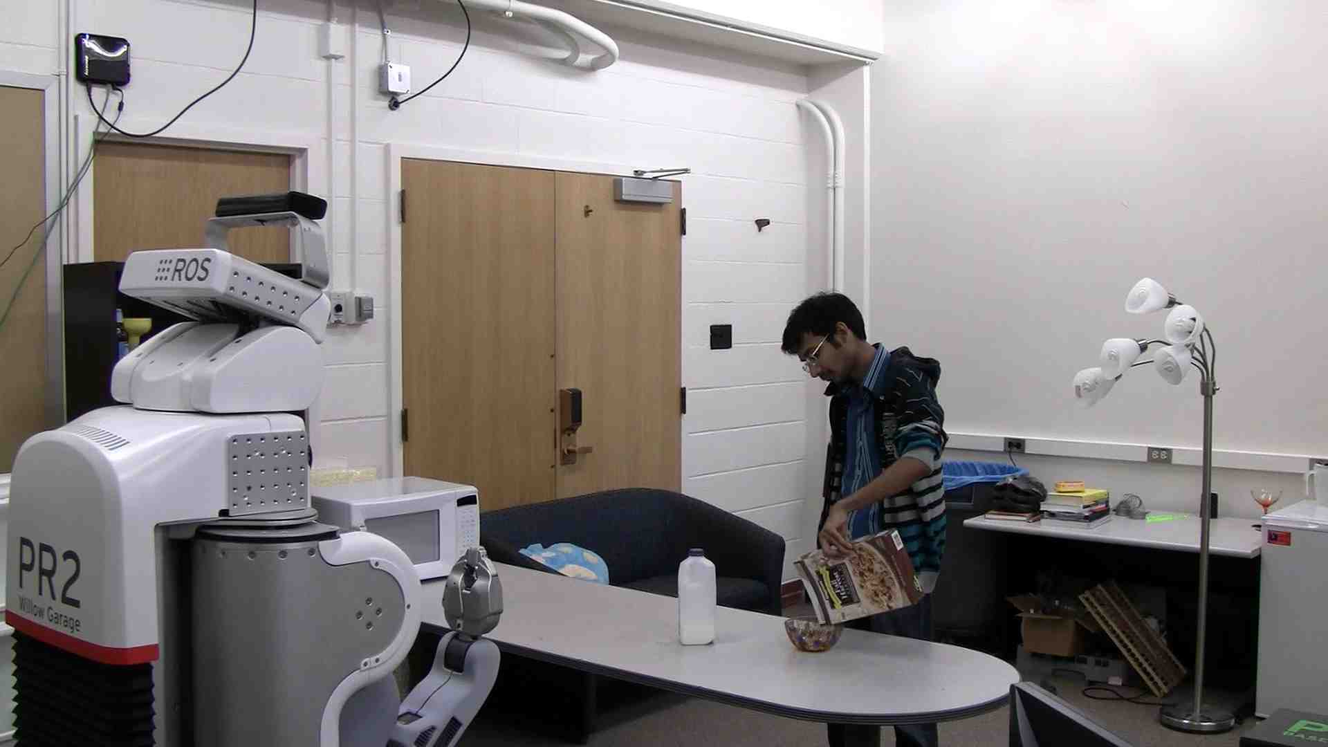
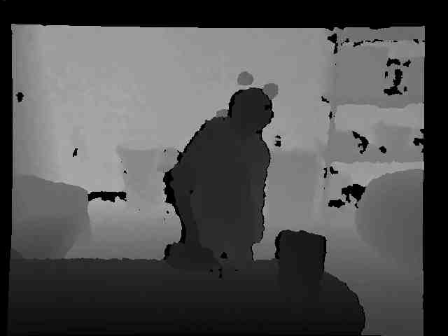
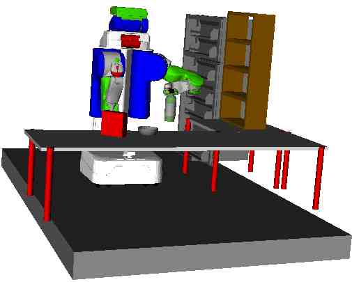
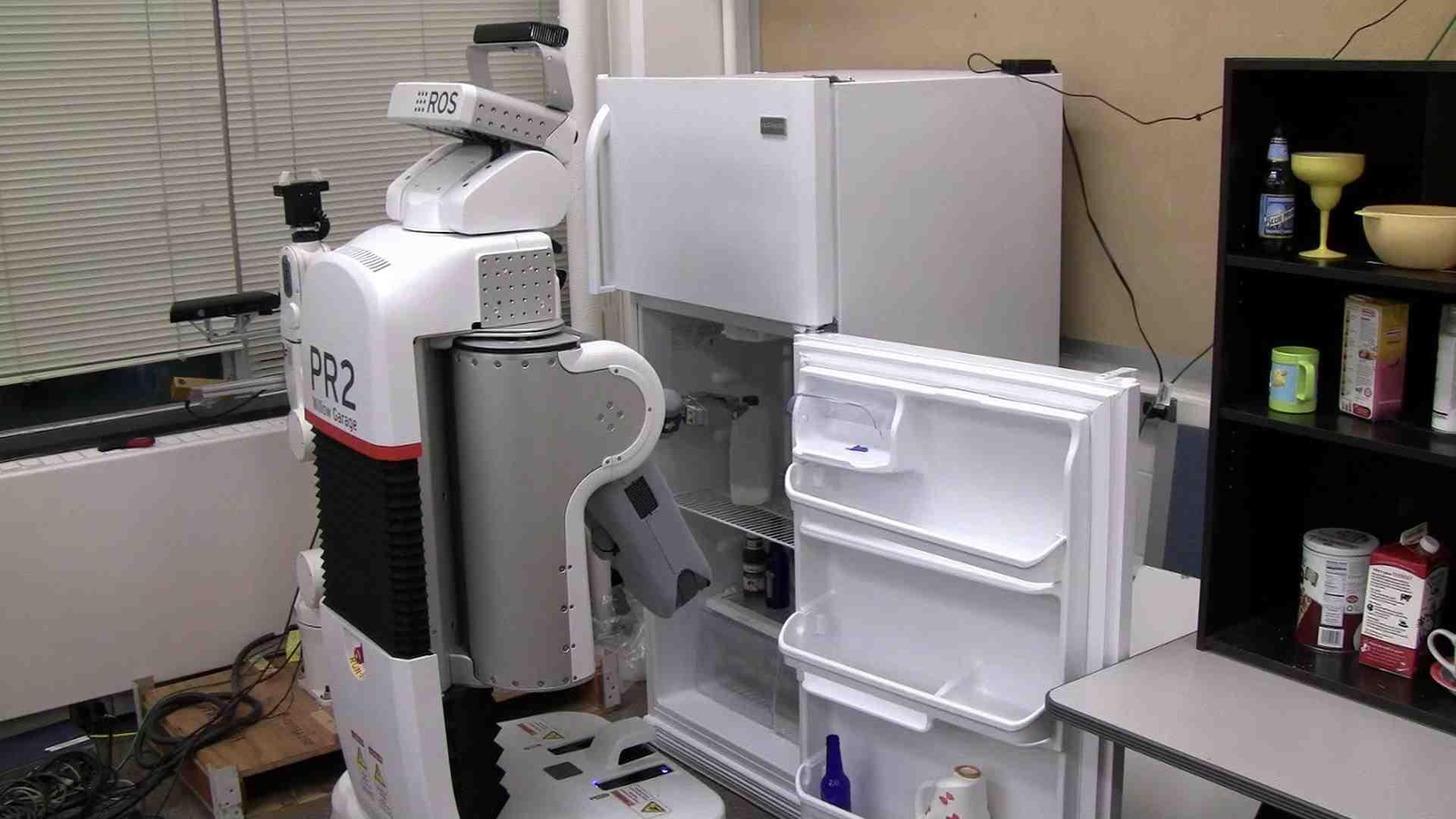
Figure 1: An assistive robot observes human activities (making cereal, top left). Using RGB-D images (top right) as input, our algorithm detects the activity being performed as well as the object affordances. This enables the robot to figure out how to interact with objects and plan actions (bottom left), and to respond appropriately to the activities being performed (cleaning up the table, bottom right).

In most previous works, object detection and activity recognition have been addressed as separate tasks. Only recently, some works have shown that modeling mutual context is beneficial (Gupta et al.,, 2009; Yao and Fei-Fei,, 2010). The key idea in our work is to note that, in activity detection, it is sometimes more informative to know how an object is being used (associated affordances, Gibson,, 1979) rather than knowing what the object is (i.e. the object category). For example, both chair and sofa might be categorized as ‘sittable,’ and a cup might be categorized as both ‘drinkable’ and ‘pourable.’ Note that the affordances of an object change over time depending on its use, e.g., a pitcher may first be reachable, then movable and finally pourable. In addition to helping activity recognition, recognizing object affordances is important by itself because of their use in robotic applications (e.g., Kormushev et al.,, 2010; Jiang et al., 2012a, ; Jiang and Saxena,, 2012).

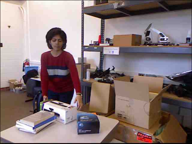
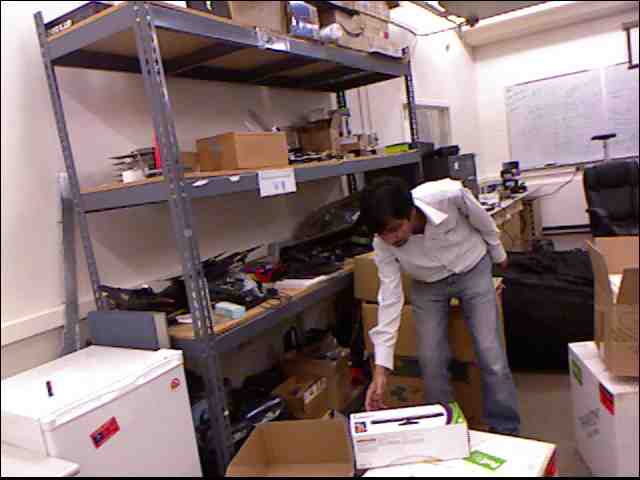
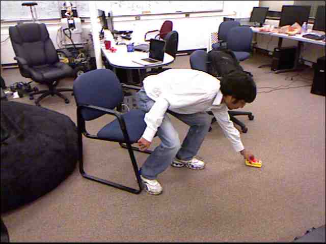
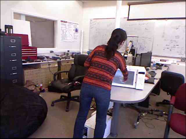
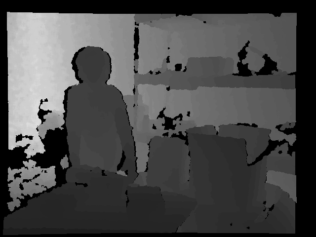
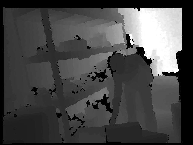
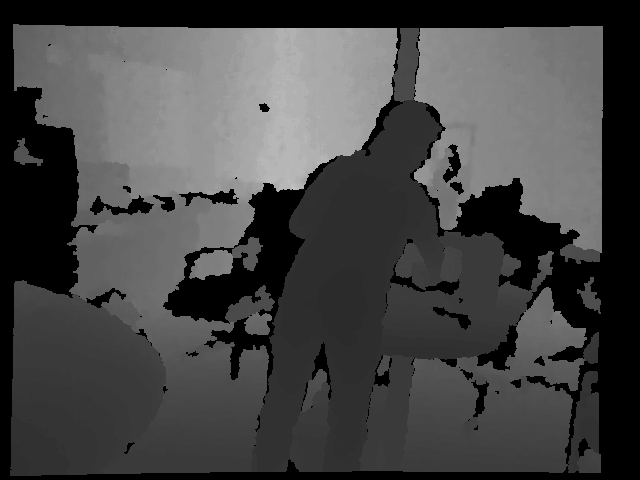
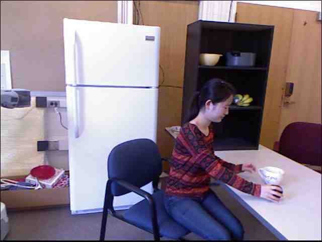
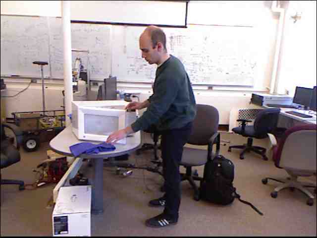
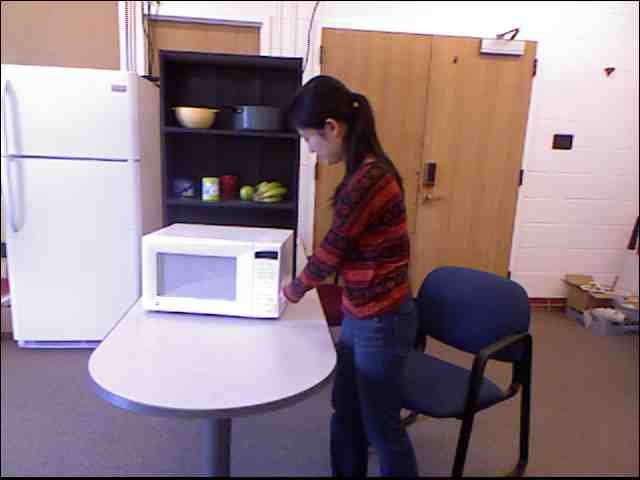
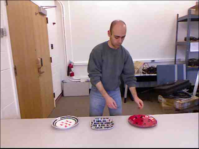
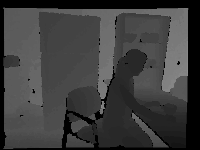
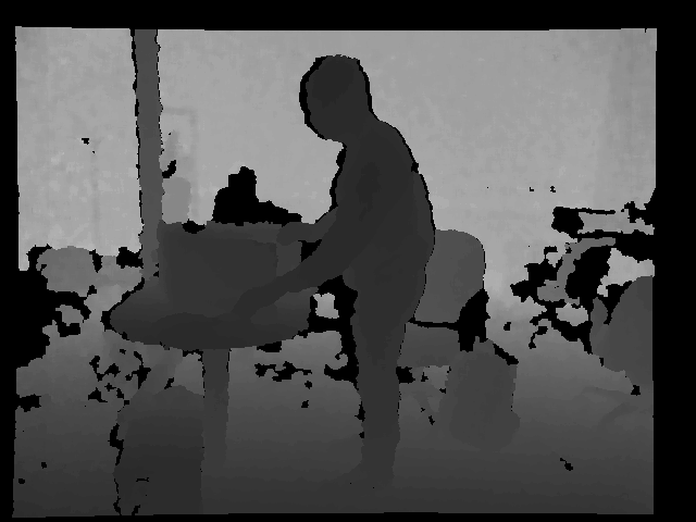
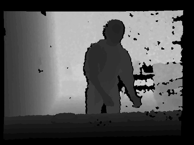
Figure 2: Significant Variations, Clutter and Occlusions: Example shots of reaching sub-activity from our dataset. First and third rows show the RGB images, and the second and bottom rows show the corresponding depth images from the RGB-D camera. Note that there are significant variations in the way the subjects perform the sub-activity. In addition, there is significant background clutter and subjects are partially occluded (e.g., column 1) or not facing the camera (e.g., row 1 column 4) in many instances.

We propose a method to learn human activities by modeling the sub-activities and affordances of the objects, how they change over time, and how they relate to each other. More formally, we define a Markov random field (MRF) over two kinds of nodes: object and sub-activity nodes. The edges in the graph model the pairwise relations among interacting nodes, namely the object–object interactions, object–sub-activity interactions, and the temporal interactions. This model is built with each spatio-temporal segment being a node. The parameters of this model are learnt using a structural support vector machine (SSVM) formulation (Finley and Joachims,, 2008). Given a new sequence of frames, we label the high-level activity, all the sub-activities and the object affordances using our learned model.

The activities take place over a long time scale, and different people execute sub-activities differently and for different periods of time. Furthermore, people also often merge two consecutive sub-activities together. Thus, segmentations in time are noisy and, in fact, there may not be one ‘correct’ segmentation, especially at the boundaries. One approach could be to consider all possible segmentations, and marginalize the segmentation; however, this is computationally infeasible. In this work, we perform sampling of several segmentations, and consider labelings over these temporal segments as latent variables in our learning algorithm.

We first demonstrate significant improvement over previous work on Cornell Activity Dataset (CAD-60). We then contribute a new dataset comprising 120 videos collected from four subjects (CAD-120). These datasets along with our code are available at http://pr.cs.cornell.edu/humanactivities/. In extensive experiments, we show that our approach outperforms the baselines in both the tasks of activity as well as affordance detection. We achieved an accuracy of 91.8% for affordance, 86.0% for sub-activity labeling and 84.7% for high-level activities respectively when given the ground truth segmentation, and an accuracy of 79.4%, 63.4% and 75.0% on these respective tasks using our multiple segmentation algorithm.

In summary, our contributions in this paper are five-fold:

• We provide a fully annotated RGB-D human activity dataset containing 120 long term activities such as making cereal, microwaving food, etc. Each video is annotated with the human skeleton tracks, object tracks, object affordance labels, sub-activity labels, and high-level activities.

• We propose a method for joint sub-activity and affordance labeling of RGB-D videos by modeling temporal and spatial interactions between humans and objects.

• We address the problem of temporal segmentation by learning the optimal labeling from multiple temporal segmentation hypotheses.

• We provide extensive analysis of our algorithms on two datasets and also demonstrate how our algorithm can be used by assistive robots.

• We release full source code along with ROS and PCL integration.

The rest of the paper is organized as follows. We start with a review of the related work in Section II. We describe the overview of our methodology in Section III and describe the model in Section IV. We then describe the object tracking and segmentation methods in Section V and VI respectively and describe the features used in our model in Section VII. We present our learning, inference and temporal segmentation algorithms in Section VIII. We present the experimental results along with robotic demonstrations in Section IX and finally conclude the paper in Section X.

II Related Work

There is a lot of recent work in improving robotic perception in order to enable the robots to perform many useful tasks. These works includes 3D modeling of indoor environments (Henry et al.,, 2012), semantic labeling of environments by modeling objects and their relations to other objects in the scene (Koppula et al.,, 2011; Lai et al., 2011b, ; Rosman and Ramamoorthy,, 2011; Anand et al.,, 2012), developing frameworks for object recognition and pose estimation for manipulation (Collet et al.,, 2011), object tracking for 3D object modeling (Krainin et al.,, 2011), etc. Robots are now becoming more integrated in human environments and are being used in assistive tasks such as automatically interpreting and executing cooking recipes (Bollini et al.,, 2012), robotic laundry folding (Miller et al.,, 2011) and arranging a disorganized house (Jiang et al., 2012b, ; Jiang and Saxena,, 2012). Such applications makes it critical for the robots to understand both object affordances as well as human activities in order to work alongside with humans. We describe the recent advances in the various aspects of this problem here.

Object affordances. An important accept of the human environment a robot needs to understand is the object affordances. Most of the work within the robotics community related to affordances has focused on predicting opportunities for interaction with an object either by using visual clues (Sun et al.,, 2009; Hermans et al.,, 2011; Aldoma et al.,, 2012) or through observation of the effects of exploratory behaviors (Montesano et al.,, 2008; Ridge et al.,, 2009; Moldovan et al.,, 2012). For instance, Sun et al., (2009) proposed a probabilistic graphical model that leverages visual object categorization for learning affordances and Hermans et al., (2011) proposed the use of physical and visual attributes as a mid-level representation for affordance prediction. Aldoma et al., (2012) proposed a method to find affordances which depends solely on the objects of interest and their position and orientation in the scene. These methods, do not consider the object affordances in human context, i.e. how the objects are usable by humans. We show that human-actor based affordances are essential for robots working in human spaces in order for them to interact with objects in a human-desirable way.

There is some recent work in interpreting human actions and interaction with objects (Lopes and Santos-Victor,, 2005; Saxena et al.,, 2008; Aksoy et al.,, 2011; Konidaris et al.,, 2012; Li et al.,, 2012) in context of learning to perform actions from demonstrations. Lopes and Santos-Victor, (2005) use context from objects in terms of possible grasp affordances to focus the attention of their action recognition system and reduce ambiguities. In contrast to these methods, we propose a model to learn human activities spanning over long durations and action-dependent affordances which make robots more capable in performing assistive tasks as we later describe in Section IX-E. Saxena et al., (2008) used supervised learning to detect grasp affordances for grasping novel objects. Li et al., (2012) used a cascaded classification model to model the interaction between objects, geometry and depths. However, their work is limited to 2D images. In recent work, Jiang et al., 2012a used a data-driven technique for learning spatial affordance maps for objects. This work is different from ours in that we consider semantic affordances with spatio-temporal grounding useful for activity detection. Pandey and Alami (2010; 2012) proposed mightability maps and taskability graphs that capture affordances such as reachability and visibility, while considering efforts required to be performed by the agents. While this work manually defines object affordances in terms of kinematic and dynamic constraints, our approach learns them from observed data.

Human activity detection from 2D videos. There has been a lot of work on human activity detection from images (Yang et al.,, 2010; Yao et al.,, 2011) and from videos (Laptev et al.,, 2008; Liu et al.,, 2009; Hoai et al.,, 2011; Shi et al.,, 2011; Matikainen et al.,, 2012; Pirsiavash and Ramanan,, 2012; Rohrbach et al.,, 2012; Sadanand and Corso,, 2012; Tang et al.,, 2012). Here, we discuss works that are closely related to ours, and refer the reader to Aggarwal and Ryoo, (2011) for a survey of the field. Most works (e.g. Hoai et al.,, 2011; Shi et al.,, 2011; Matikainen et al.,, 2012) consider detecting actions at a ‘sub-activity’ level (e.g. walk, bend, and draw) instead of considering high-level activities. Their methods range from discriminative learning techniques for joint segmentation and recognition (Shi et al.,, 2011; Hoai et al.,, 2011) to combining multiple models (Matikainen et al.,, 2012). Some works, such as Tang et al., (2012), consider high-level activities. Tang et al., (2012) proposed a latent model for high-level activity classification and have the advantage of requiring only high-level activity labels for learning. None of these methods explicitly consider the role of objects or object affordances that not only help in identifying sub-activities and high-level activities, but are also important for several robotic applications (e.g. Kormushev et al.,, 2010).

Some recent works (Gupta et al.,, 2009; Yao and Fei-Fei,, 2010; Aksoy et al.,, 2010; Jiang et al., 2011a, ; Pirsiavash and Ramanan,, 2012) show that modeling the interaction between human poses and objects in 2D videos results in a better performance on the tasks of object detection and activity recognition. However, these works cannot capture the rich 3D relations between the activities and objects, and are also fundamentally limited by the quality of the human pose inferred from the 2D data. More importantly, for activity recognition, the object affordance matters more than its category.

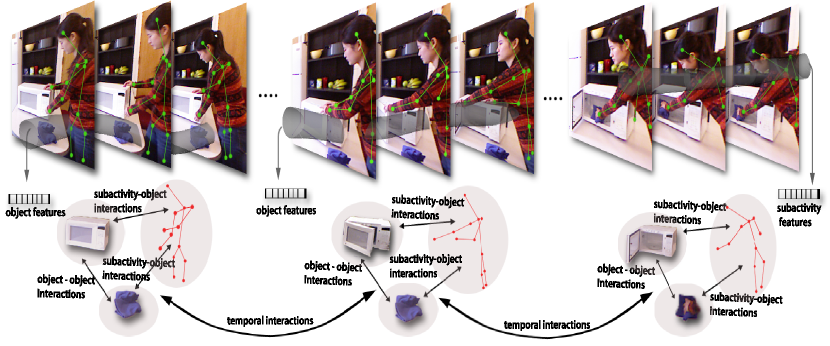
Figure 3: Pictorial representation of the different types of nodes and relationships modeled in part of the cleaning objects activity comprising three sub-activities: reaching, opening and scrubbing. (See Section III.)

Kjellström et al., (2011) used a factorial CRF to simultaneously segment and classify human hand actions, as well as classify the object affordances involved in the activity from 2D videos. However, this work is limited to classifying only hand actions and does not model interactions between the objects. We consider complex full-body activities and show that modeling object–object interactions is important as objects have affordances even if they are not directly interacted with human hands.

Human activity detection from RGB-D videos. Recently, with the availability of inexpensive RGB-D sensors, some works (Li et al.,, 2010; Ni et al.,, 2011; Sung et al.,, 2011; Zhang and Parker,, 2011; Sung et al.,, 2012) consider detecting human activities from RGB-D videos. Li et al., (2010) proposed an expandable graphical model, to model the temporal dynamics of actions and use a bag of 3D points to model postures. They use their method to classify 20 different actions which are used in context of interacting with a game console, such as draw tick, draw circle, hand clap, etc. Zhang and Parker, (2011) designed 4D local spatio-temporal features and use an LDA classifier to identify six human actions such as lifting, removing, waving, etc., from a sequence of RGB-D images. However, both these works only address detecting actions which span short time periods. Ni et al., (2011) also designed feature representations such as spatio-temporal interest points and motion history images which incorporate depth information in order to achieve better recognition performance. Panangadan et al., (2010) used data from laser rangefinder to model observed movement patterns and interactions between persons. They segment tracks into activities based on difference in displacement distributions in each segment, and use a Markov model for capturing the transition probabilities. None of these works model interactions with objects which provide useful information for recognizing complex activities.

In recent previous work from our lab, Sung et al., (2011, 2012) proposed a hierarchical maximum entropy Markov model to detect activities from RGB-D videos and treat the sub-activities as hidden nodes in their model. However, they use only human pose information for detecting activities and also constrain the number of sub-activities in each activity. In contrast, we model context from object interactions along with human pose, and also present a better learning algorithm. (See Section IX for further comparisons.) Gall et al., (2011) also use depth data to perform sub-activity (referred to as action) classification and functional categorization of objects. Their method first detects the sub-activity being performed using the estimated human pose from depth data, and then performs object localization and clustering of the objects into functional categories based on the detected sub-activity. In contrast, our proposed method performs joint sub-activity and affordance labeling and uses these labels to perform high-level activity detection.

All of the above works lack a unified framework that combines all of the information available in human interaction activities and therefore we propose a model that captures both the spatial and temporal relations between object affordances and human poses to perform joint object affordance and activity detection.

III Overview

Over the course of a video, a human may interact with several objects and perform several sub-activities over time. In this section we describe at a high level how we process the RGB-D videos and model the various properties for affordance and activity labeling.

Given the raw data containing the color and depth values for every pixel in the video, we first track the human skeleton using Openni’s skeleton tracker for obtaining the locations of the various joints of the human skeleton. However these values are not very accurate, as the Openni’s skeleton tracker is only designed to track human skeletons in clutter-free environments and without any occlusion of the body parts. In real-world human activity videos, some body parts are often occluded and the interaction with the objects hinders accurate skeleton tracking. We show that even with such noisy data, our method gets high accuracies by modeling the mutual context between the affordances and sub-activities.

We then segment the object being used in the activity and track them through out the 3D video, as explained in detail in Section V. We model the activities and affordances by defining a MRF over the spatio-temporal sequence we get from an RGB-D video, as illustrated in Fig. 3. MRFs are a workhorse of machine learning, and have been successfully applied to many applications (e.g. Saxena et al.,, 2009). Please see Koller and Friedman, (2009) for a review. If we build our graph with nodes for objects and sub-activities for each time instant (at 30 fps), then we will end up with quite a large graph. Furthermore, such a graph would not be able to model meaningful transitions between the sub-activities because they take place over a long-time (e.g. a few seconds). Therefore, in our approach we first segment the video into small temporal segments, and our goal is to label each segment with appropriate labels. We try to over-segment, so that we end up with more segments and avoid merging two sub-activities into one segment. Each of these segments occupies a small length of time and therefore, considering nodes per segment gives us a meaningful and concise representation for the graph $\mathcal{G}$. With such a representation, we can model meaningful transitions of a sub-activity following another, e.g. pouring followed by moving. Our temporal segmentation algorithms are described in Section VI. The outputs from the skeleton and object tracking along with the segmentation information and RGB-D videos are then used to generate the features described in Section VII.

Given the tracks and segmentation, the graph structure ($\mathcal{G}$) is constructed with a node for each object and a node for the sub-activity of a temporal segment, as shown in Fig. 3. The nodes are connected to each other within a temporal segment and each node is connected to its temporal neighbors by edges as further described in Section IV. The learning and inference algorithms for our model are presented in Section VIII. We capture the following properties in our model:

• Affordance–sub-activity relations. At any given time, the affordance of the object depends on the sub-activity it is involved in. For example, a cup has the affordance of ‘pour-to’ in a pouring sub-action and has the affordance of ‘drinkable’ in a drinking sub-action. We compute relative geometric features between the object and the human’s skeletal joints to capture this. These features are incorporated in the energy function as described in Eq. (6).

• Affordance–affordance relations. Objects have affordances even if they are not interacted directly with by the human, and their affordances depend on the affordances of other objects around them. For example, in the case of pouring from a pitcher to a cup, the cup is not interacted with by the human directly but has the affordance ‘pour-to’. We therefore use relative geometric features such as ‘on top of’, ‘nearby’, ‘in front of’, etc., to model the affordance–affordance relations. These features are incorporated in the energy function as described in Eq. (5).

• Sub-activity change over time. Each activity consists of a sequence of sub-activities that change over the course of performing the activity. We model this by incorporating temporal edges in $\mathcal{G}$. Features capturing the change in human pose across the temporal segments are used to model the sub-activity change over time and the corresponding energy term is given in Eq. (8).

• Affordance change over time. The object affordances depend on the sub-activity being performed and hence change along with the sub-activity over time. We model the temporal change in affordances of each object using features such as change in appearance and location of the object over time. These features are incorporated in the energy function as described in Eq. (7).

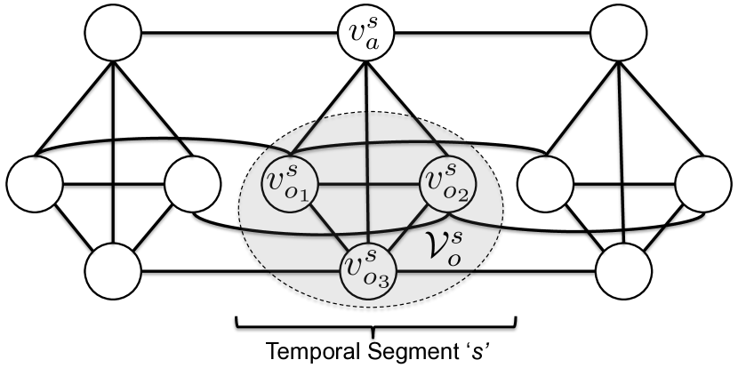
Figure 4: An illustrative example of our Markov random field (MRF) for three temporal segments, with one activity node, $v^{s}_{a}$, and three object nodes, {$v^{s}_{o_{1}}$,$v^{s}_{o_{2}}$,$v^{s}_{o_{3}}$}, per temporal segment.

IV Model

Our goal is to perform joint activity and object affordance labeling of RGB-D videos. We model the spatio-temporal structure of an activity using a model isomorphic to a MRF with log-linear node and pairwise edge potentials (see Fig. 3 and 4 for an illustration). The MRF is represented as a graph $\mathcal{G}=(\mathcal{V},\mathcal{E})$. Given a temporally segmented 3D video, with temporal segments $s\in\{1,...,N\}$, our goal is to predict a labeling ${\mathbf{y}}=({\mathbf{y}_{1}},...,{\mathbf{y}_{N}})$ for the video, where ${\mathbf{y}_{s}}$ is the set of sub-activity and object affordance labels for the temporal segment $s$. Our input is a set of features ${\mathbf{x}}$ extracted from the segmented 3D video as described in Section VII. The prediction $\hat{{\mathbf{y}}}$ is computed as the argmax of a energy function ${E_{{\mathbf{w}}}({\mathbf{x}},{\mathbf{y}})}$ that is parameterized by weights ${\mathbf{w}}$.

$$\hat{{\mathbf{y}}} =\operatorname*{argmax}_{\mathbf{y}}{E_{{\mathbf{w}}}({\mathbf{x}},{\mathbf{y}})}$$ (1)

$${E_{{\mathbf{w}}}({\mathbf{x}},{\mathbf{y}})} =E_{o}+E_{a}+E_{oo}+E_{oa}+E^{t}_{oo}+E^{t}_{aa}$$ (2)

The energy function consists of six types of potentials that define the energy of a particular assignment of sub-activity and object affordance labels to the sequence of segments in the given video. The various potentials capture the dependencies between the sub-activity and object affordance labels as defined by an undirected graph $\mathcal{G}=(\mathcal{V},\mathcal{E})$.

We now describe the structure of this graph along with the corresponding potentials. There are two types of nodes in $\mathcal{G}$: object nodes denoted by $\mathcal{V}_{o}$ and sub-activity nodes denoted by $\mathcal{V}_{a}$. Let $K_{a}$ denote the set of sub-activity labels, and $K_{o}$ denote the set of object affordance labels. Let ${y_{i}^{k}}$ be a binary variable representing the node $i$ having label $k$, where $k\in K_{o}$ for object nodes and $k\in K_{a}$ for sub-activity nodes. All $k$ binary variables together represent the label of a node. Let $\mathcal{V}_{o}^{s}$ denote set of object nodes of segment $s$, and $v_{a}^{s}$ denote the sub-activity node of segment $s$. Figure 4 shows the graph structure for three temporal segments for an activity with three objects.

The energy term associated with labeling the object nodes is denoted by $E_{o}$ and is defined as the sum of object node potentials $\psi_{o}(i)$ as:

$$E_{o}=\sum_{i\in\mathcal{V}_{o}}\psi_{o}(i)=\sum_{i\in\mathcal{V}_{o}}\sum_{k\in K_{o}}{y_{i}^{k}}\left[{\mathbf{w}_{\mathbf{o}}^{k}}\cdot{\phi_{o}({i})}\right],$$ (3)

where ${\phi_{o}({i})}$ denotes the feature map describing the object affordance of the object node $i$ in its corresponding temporal segment through a vector of features, and there is one weight vector for each affordance class in $K_{o}$. Similarly, we have an energy term, $E_{a}$, for labeling the sub-activity nodes which is defined as the sum of sub-activity node potentials as

$$E_{a}=\sum_{i\in\mathcal{V}_{a}}\psi_{a}(i)=\sum_{i\in\mathcal{V}_{a}}\sum_{k\in K_{a}}{y_{i}^{k}}\left[{\mathbf{w}_{\mathbf{a}}^{k}}\cdot{\phi_{a}({i})}\right],$$ (4)

where ${\phi_{a}({i})}$ denotes the feature map describing the sub-activity node $i$ through a vector of features, and there is one weight vector for each sub-activity class in $K_{a}$.

For all segments $s$, there is an edge connecting all the nodes in $\mathcal{V}_{o}^{s}$ to each other, denoted by $\mathcal{E}_{oo}$, and to the sub-activity node $v_{a}^{s}$, denoted by $\mathcal{E}_{oa}$. These edges signify the relationships within the objects, and between the objects and the human pose within a segment and are referred to as ‘object–object interactions’ and ‘sub-activity–object interactions’ in the Fig. 3, respectively.

The sub-activity node of segment $s$ is connected to the sub-activity nodes in segments $(s-1)$ and $(s+1)$. These temporal edges are denoted by $\mathcal{E}^{t}_{aa}$. Similarly every object node of segment $s$ is connected to the corresponding object nodes in segments $(s-1)$ and $(s+1)$, denoted by $\mathcal{E}^{t}_{oo}$. These edges model the temporal interactions between the human poses and the objects, respectively, and are represented by dotted edges in the Fig. 3.

We have one energy term for each of the four interaction types and are defined as:

$$E_{oo} =\sum_{(i,j)\in\mathcal{E}_{oo}}\sum_{(l,k)\in K_{o}\times K_{o}}{y_{i}^{l}}{y_{j}^{k}}\left[{\mathbf{w}_{\mathbf{oo}}^{lk}}\cdot{\phi_{oo}(i,j)}\right],$$ (5)

$$E_{oa} =\sum_{(i,j)\in\mathcal{E}_{oa}}\sum_{(l,k)\in K_{o}\times K_{a}}{y_{i}^{l}}{y_{j}^{k}}\left[{\mathbf{w}_{\mathbf{oa}}^{lk}}\cdot{\phi_{oa}(i,j)}\right],$$ (6)

$$E^{t}_{oo} =\sum_{(i,j)\in\mathcal{E}^{t}_{oo}}\sum_{(l,k)\in K_{o}\times K_{o}}{y_{i}^{l}}{y_{j}^{k}}\left[{\mathbf{w^{t}}_{\mathbf{oo}}^{lk}}\cdot{\phi^{t}_{oo}(i,j)}\right],$$ (7)

$$E^{t}_{aa} =\sum_{(i,j)\in\mathcal{E}^{t}_{aa}}\sum_{(l,k)\in K_{a}\times K_{a}}{y_{i}^{l}}{y_{j}^{k}}\left[{\mathbf{w^{t}}_{\mathbf{aa}}^{lk}}\cdot{\phi^{t}_{aa}(i,j)}\right].$$ (8)

The feature maps ${\phi_{oo}(i,j)}$ and ${\phi_{oa}(i,j)}$ describe the interactions between pair of objects and interactions between an object and the human skeleton within a temporal segment, respectively, and the feature maps ${\phi^{t}_{oo}(i,j)}$ and ${\phi^{t}_{aa}(i,j)}$ describe the temporal interactions between objects and sub-activities, respectively. Also, note that there is one weight vector for every pair of labels in each energy term.

Given $\mathcal{G}$, we can rewrite the energy function based on individual node potentials and edge potentials compactly as follows:

$${E_{{\mathbf{w}}}({\mathbf{x}},{\mathbf{y}})} =\sum_{i\in\mathcal{V}_{a}}\sum_{k\in K_{a}}{y_{i}^{k}}\left[{\mathbf{w}_{\mathbf{a}}^{k}}\cdot{\phi_{a}({i})}\right]+\sum_{i\in\mathcal{V}_{o}}\sum_{k\in K_{o}}{y_{i}^{k}}\left[{\mathbf{w}_{\mathbf{o}}^{k}}\cdot{\phi_{o}({i})}\right]$$

$$+\sum_{t\in{\cal T}}\sum_{(i,j)\in\mathcal{E}_{t}}\sum_{(l,k)\in T_{t}}{y_{i}^{l}}{y_{j}^{k}}\left[{\mathbf{w}_{\mathbf{t}}^{lk}}\cdot{\phi_{t}(i,j)}\right]$$ (9)

where $\cal T$ is the set of the four edge types described above. Writing the energy function in this form allows us to apply efficient inference and learning algorithms as described later in Section VIII.

V Object Detection and Tracking

For producing our graph $\mathcal{G}$, we need as input the segments corresponding to the objects (but not their labels) and their tracks over time. In order to do so, we run pre-trained object detectors on a set of frames sampled from the video and then use particle filter tracker to obtain tracks of the detected objects. We then find consistent tracks that connect the various detected objects in order to find reliable object tracks. We present the details below.

Object Detection: We first train a set of 2D object detectors for the common objects present in our dataset (e.g. mugs, bowls). We use features that capture the inherent local and global properties of the object encompassing the appearance and the shape/geometry. Local features includes color histogram and the histogram of oriented gradients (HoG, Dalal and Triggs,, 2005) which provide the intrinsic properties of the target object while viewpoint features histogram (VFH, Rusu et al.,, 2010) provides the global orientation of the normals from the object’s surface. For training we used the RGB-D object dataset by Lai et al., 2011a and built a one-vs-all SVM classifier using the local features for each object class in order to obtain the probability estimates of each object class. We also build a k-nearest neighbor (kNN) classifier over VFH features. The kNN classifier provides the detection score as inverse of the distance between training and the test instance. We obtain a final classification score by adding the scores from these two classifiers.

At test time, for a given point cloud, we first reduce the set of 3D bounding boxes by only considering those that belong to a volume around the hands of the skeleton. This reduces the number of false detections as well as the detection time. We then run our SVM-based object detectors on the RGB image. This gives us the exact $x$ and $y$ coordinates of the possible detections. The predictions with score above a certain threshold are further examined by calculating the kNN score based on VFH features. To find the exact depth of the object, we do pyramidal window search inside the current 3D bounding box and get the highest scoring box. In order to remove the empty space and any outlier points within a bounding box, we shrink it towards the highest-density region that captures 90% of the object points. These bounding box detections are ordered according to their final classification score.

Object Tracking: We used the particle filter tracker implementation provided under the PCL library for tracking our target object. The tracker uses the color values and the normals to find the next probable state of the object.

Combining Object Detections with Tracking: We take the top detections, track them, and assign a score to each of them in order to compute the potential nodes in the graph $\mathcal{G}$.

We start with building a graph with the initial bounding boxes as the nodes. In our current implementation, this method needs an initial guess on the 2D bounding boxes of the objects to keep the algorithm tractable. We can obtain this by considering only the tabletop objects by using a tabletop object segmenter (e.g. Rusu et al.,, 2009). We initialize the graph with these guesses. We then perform tracking through the video and grow the graph by adding a node for every object detection and connect two nodes with an edge if a track exists between their corresponding bounding boxes. Our object detection algorithm is run after every fixed number of frames, and the frames on which it is run are referred to as the detection frames. Each edge is assigned a weight corresponding to its track score as defined in Eq. (10). After the whole video is processed, the best track for every initial node in the graph is found by taking the highest weighted path starting at that node.

The object detections at the current frame are categorized into one of the following categories: {merged detection, isolated detection, ignored detection} based on their vicinity and similarity to the currently tracked objects as shown in Figure 5. If a detection occurs close to a currently tracked object and has high similarity with it, the detection can be merged with the current object track. Such detections are called merged detections. The detections which have high detection score but do not occur close to the current tracks are labeled as isolated detections and are tracked in both directions. This helps in correcting the tracks which have gone wrong due to partial occlusions or missing due to full occlusions of the objects. The rest of the detections are labeled as ignored detections and are not tracked.

Figure 5: Pictorial representation of our algorithm for combining object detections with tracking.

More formally, let $d^{i}_{j}$ represent the bounding box of the $j^{th}$ detection in the $i^{th}$ detection frame and let $D^{i}_{j}$ represent its tracking score. Let $\hat{d}^{i}_{j}$ represent the tracked bounding box at the current frame with the track starting from $d^{i}_{j}$. We define a similarity score, $S(a,b)$, between two image bounding boxes, $a$ and $b$, as the correlation score of the color histograms of the two bounding boxes. The track score of an edge $e$ connecting the detections $d^{i-1}_{k}$ and $d^{i}_{j}$ is given by

$$ts(e)=S(d^{i-1}_{k},d^{i}_{j})+S(\hat{d}^{i-1}_{k},d^{i}_{j})+\lambda D^{i}_{j}$$ (10)

Finally, the best track of a given object bounding box $b$ is the path having the highest cumulative track score from all paths originating at node corresponding to $b$ in the graph, represented by the set $P_{b}$

$$\hat{t}(b)=\operatorname*{argmax}_{p\in P_{b}}\sum\limits_{e\in p}ts(e).$$ (11)

VI Temporal Segmentation

We perform temporal segmentation of the frames in an activity in order to obtain groups of frames representing atomic movements of the human skeleton and objects in the activity. This will group similar frames into one segment, thus reducing the total number of nodes to be considered by the learning algorithm significantly.

There are several problems with naively performing one temporal segmentation—if we make a mistake here, then our followup activity detection would perform poorly. In certain cases, when the features are additive, methods based on dynamic programming (Hoai et al.,, 2011; Shi et al.,, 2011; Hoai and De la Torre,, 2012) could be used to search for an optimal segmentation.

However, in our case, we have the following three challenges. First, the feature maps we consider are non-additive in nature, and the feature computation cost is exponential in the number of frames if we want to consider all the possible segmentations. Therefore, we cannot apply dynamic programming techniques to find the optimal segmentation. Second, the complex human-object interactions are poorly approximated with a linear dynamical system, therefore techniques such as Fox et al., (2011) cannot be directly applied. Third, the boundary between two sub-activities is often not very clear, as people often start performing the next sub-activity before finishing the current sub-activity. The amount of overlap might also depend on which sub-activities are being performed. Therefore, there may not be one optimal segmentation. In our work, we consider several temporal segmentations and propose a method to combine them in Section VIII-C.

We consider three basic methods for temporal segmentation of the video frames and generate a number of temporal segmentations by varying the parameters of these methods. The first method is uniform segmentation, in which we consider a set of continuous frames of fixed size as the temporal segment. There are two parameters for this method: the segment size and the offset (the size of the first segment). The other two segmentation methods use the graph-based segmentation proposed by Felzenszwalb and Huttenlocher, (2004) adapted to temporally segment the videos. The second method uses the sum of the Euclidean distances between the skeleton joints as the edge weights, whereas the third method uses the rate of change of the Euclidean distance as the edge weights. These methods consider smooth movements of the skeleton joints to belong to one segment and identify sudden changes in skeletal motion as the sub-activity boundaries.

In detail, we have one node per frame representing the skeleton in the graph based methods. Each node is connected to its temporal neighbor, therefore giving a chain graph. The algorithm begins with having each node as a separate segmentation, and iteratively merges the components if the edge weight is less than a certain threshold (computed based on the current segment size and a constant parameter). We obtain different segmentations by varying the parameter.

VII Features

TABLE I: Summary of the Features used in the Energy Function.

Description	Count
Object Features	18
N1. Centroid location	3
N2. 2D bounding box	4
N3. Transformation matrix of SIFT matches between adjacent frames	6
N4. Distance moved by the centroid	1
N5. Displacement of centroid	1
Sub-activity Features	103
N6. Location of each joint (8 joints)	24
N7. Distance moved by each joint (8 joints)	8
N8. Displacement of each joint (8 joints)	8
N9. Body pose features	47
N10. Hand position features	16
Object-object Features (computed at start frame, middle frame, end frame, max and min)	20
E1. Difference in centroid locations $(\Delta x,\Delta y,\Delta z)$	3
E2. Distance between centroids	1
Object–sub-activity Features (computed at start frame, middle frame, end frame, max and min)	40
E3. Distance between each joint location and object centroid	8
Object Temporal Features	4
E4. Total and normalized vertical displacement	2
E5. Total and normalized distance between centroids	2
Sub-activity Temporal Features	16
E6. Total and normalized distance between each corresponding joint locations (8 joints)	16

For a given object node $i$, the node feature map ${\phi_{o}({i})}$ is a vector of features representing the object’s location in the scene and how it changes within the temporal segment. These features include the $(x,y,z)$ coordinates of the object’s centroid and the coordinates of the object’s bounding box at the middle frame of the temporal segment. We also run a SIFT feature based object tracker (Pele and Werman,, 2008) to find the corresponding points between the adjacent frames and then compute the transformation matrix based on the matched image points. We add the transformation matrix corresponding to the object in the middle frame with respect to its previous frame to the features in order to capture the object’s motion information. In addition to the above features, we also compute the total displacement and the total distance moved by the object’s centroid in the set of frames belonging to the temporal segment. We then perform cumulative binning of the feature values into 10 bins. In our experiments, we have ${\phi_{o}({i})}\in\mathbb{R}^{180}$.

Similarly, for a given sub-activity node $i$, the node feature map ${\phi_{a}({i})}$ gives a vector of features computed using the human skeleton information obtained from running Openni’s skeleton tracker on the RGB-D video. We compute the features described above for each of the upper-skeleton joint (neck, torso, left shoulder, left elbow, left palm, right shoulder, right elbow and right palm) locations relative to the subject’s head location. In addition to these, we also consider the body pose and hand position features as described by Sung et al., (2012), thus giving us ${\phi_{a}({i})}\in\mathbb{R}^{1030}$.

The edge feature maps ${\phi_{t}(i,j)}$ describe the relationship between node $i$ and $j$. They are used for modeling four types of interactions: object–object within a temporal segment, object–sub-activity within a temporal segment, object–object between two temporal segments, and sub-activity–sub-activity between two temporal segments. For capturing the object-object relations within a temporal segment, we compute relative geometric features such as the difference in $(x,y,z)$ coordinates of the object centroids and the distance between them. These features are computed at the first, middle and last frames of the temporal segment along with minimum and maximim of their values across all frames in the temporal segment to capture the relative motion information. This gives us ${\phi_{1}(i,j)}\in\mathbb{R}^{200}$. Similarly for object–sub-activity relation features ${\phi_{2}(i,j)}\in\mathbb{R}^{400}$, we use the same features as for the object–object relation features, but we compute them between the upper-skeleton joint locations and each object’s centroid. The temporal relational features capture the change across temporal segments and we use the vertical change in position and the distance between the corresponding object and the joint locations. This gives us ${\phi_{3}(i,j)}\in\mathbb{R}^{40}$ and ${\phi_{4}(i,j)}\in\mathbb{R}^{160}$ respectively.

VIII Inference and Learning Algorithm

VIII-A Inference.

Given the model parameters $w$, the inference problem is to find the best labeling $\hat{{\mathbf{y}}}$ for a new video ${\mathbf{x}}$, i.e. solving the argmax in Eq. (1) for the discriminant function in Eq. (9). This is a NP hard problem. However, its equivalent formulation as the following mixed-integer program has a linear relaxation which can be solved efficiently as a quadratic pseudo-Boolean optimization problem using a graph-cut method (Rother et al.,, 2007).

$$\hat{{\mathbf{y}}}\!=\!\operatorname*{argmax}_{{\mathbf{y}}}\max_{\mathbf{z}}\sum_{i\in\mathcal{V}_{a}}\sum_{k\in K_{a}}{y_{i}^{k}}\left[{\mathbf{w}_{\mathbf{a}}^{k}}\cdot{\phi_{a}({i})}\right]+\!\!\!\sum_{i\in\mathcal{V}_{o}}\sum_{k\in K_{o}}{y_{i}^{k}}\left[{\mathbf{w}_{\mathbf{o}}^{k}}\cdot{\phi_{o}({i})}\right]$$

$$\qquad\qquad\qquad\quad+\sum_{t\in{\cal T}}\sum_{(i,j)\in\mathcal{E}_{t}}\sum_{(l,k)\in T_{t}}{z_{ij}^{lk}}\left[{\mathbf{w}_{\mathbf{t}}^{lk}}\cdot{\phi_{t}(i,j)}\right]$$ (12)

$$\forall i,j,l,k\!:\>\>{z_{ij}^{lk}}\leq{y_{i}^{l}},\>\>{z_{ij}^{lk}}\leq{y_{j}^{k}},\>\>{y_{i}^{l}}+{y_{j}^{k}}\leq{z_{ij}^{lk}}+1,\>\>{z_{ij}^{lk}},{y_{i}^{l}}\in\{0,1\}$$ (13)

Note that the products ${y_{i}^{l}}{y_{j}^{k}}$ have been replaced by auxiliary variables $z^{lk}_{ij}$. Relaxing the variables ${z_{ij}^{lk}}$ and ${y_{i}^{l}}$ to the interval $[0,1]$ results in a linear program that can be shown to always have half-integral solutions (i.e. ${y_{i}^{l}}$ only take values $\{0,0.5,1\}$ at the solution) (Hammer et al.,, 1984). Since every node in our experiments has exactly one class label, we also consider the linear relaxation from above with the additional constraints $\forall i\in\mathcal{V}_{a}:\sum_{l\in K_{a}}{y_{i}^{l}}=1$ and $\forall i\in\mathcal{V}_{o}:\sum_{l\in K_{o}}{y_{i}^{l}}=1$. This problem can no longer be solved via graph cuts. We compute the exact mixed integer solution including these additional constraint using a general-purpose MIP solver during inference.

In our experiments, we obtain a processing rate of 74.9 frames/second for inference and 16.0 frames/second end-to-end (including feature computation cost) on a 2.93 GHz Intel processor with 16 GB of RAM on Linux. In detail, the MIP solver takes 6.94 seconds for a typical video with 520 frames and the corresponding graph has 12 sub-activity nodes and 36 object nodes, i.e. 15908 variables. This is the time corresponding to solving the argmax in Eq. (12-13) and does not involve the feature computation time. The time taken for end-to-end classification including feature generation is 32.5 seconds.

VIII-B Learning.

We take a large-margin approach to learning the parameter vector ${\mathbf{w}}$ of Eq. (9) from labeled training examples $({\mathbf{x}}_{1},{\mathbf{y}}_{1}),...,({\mathbf{x}}_{M},{\mathbf{y}}_{M})$ (Taskar et al.,, 2004; Tsochantaridis et al.,, 2004). Our method optimizes a regularized upper bound on the training error

$$\textstyle R(h)=\frac{1}{{M}}\sum_{m=1}^{{M}}{\Delta({\mathbf{y}}_{m},\hat{{\mathbf{y}}}_{m})},$$

where $\hat{{\mathbf{y}}}_{m}$ is the optimal solution of Eq. (1) and ${\Delta({\mathbf{y}},\hat{{\mathbf{y}}})}$ is the loss function defined as

$$\textstyle{\Delta({\mathbf{y}},\hat{{\mathbf{y}}})}=\sum_{i\in\mathcal{V}_{o}}\sum_{k\in K_{o}}|{y_{i}^{k}}-\hat{y}_{i}^{k}|+\sum_{i\in\mathcal{V}_{a}}\sum_{k\in K_{a}}|{y_{i}^{k}}-\hat{y}_{i}^{k}|.$$

To simplify notation, note that Eq. (12) can be equivalently written as ${\mathbf{w}}^{T}\Psi({\mathbf{x}},{\mathbf{y}})$ by appropriately stacking the ${\mathbf{w}_{\mathbf{a}}^{k}}$ , ${\mathbf{w}_{\mathbf{o}}^{k}}$ and ${\mathbf{w}_{\mathbf{t}}^{lk}}$ into ${\mathbf{w}}$ and the ${y_{i}^{k}}{\phi_{a}({i})}$, ${y_{i}^{k}}{\phi_{o}({i})}$ and ${z_{ij}^{lk}}{\phi_{t}(i,j)}$ into $\Psi({\mathbf{x}},{\mathbf{y}})$, where each ${z_{ij}^{lk}}$ is consistent with Eq. (13) given ${\mathbf{y}}$. Training can then be formulated as the following convex quadratic program (Joachims et al.,, 2009):

$$\min_{w,\xi} \frac{1}{2}{\mathbf{w}}^{T}{\mathbf{w}}+C\xi$$ (14)

$$s.t. \forall\bar{{\mathbf{y}}}_{1},...,\bar{{\mathbf{y}}}_{M}\in\{0,0.5,1\}^{N\cdot K}:$$

$$\frac{1}{M}{\mathbf{w}}^{T}\sum_{m=1}^{M}[\Psi({\mathbf{x}}_{m},{\mathbf{y}}_{m})-\Psi({\mathbf{x}}_{m},\bar{{\mathbf{y}}}_{m})]\geq\Delta({\mathbf{y}}_{m},\bar{{\mathbf{y}}}_{m})-\xi$$

While the number of constraints in this QP is exponential in ${M}$, $N$ and $K$, it can nevertheless be solved efficiently using the cutting-plane algorithm (Joachims et al.,, 2009). The algorithm needs access to an efficient method for computing

$$\bar{{\mathbf{y}}}_{m} = \!\!\!\!\!\operatorname*{argmax}_{{\mathbf{y}}\in\{0,0.5,1\}^{N\cdot K}}\left[{\mathbf{w}}^{T}\Psi({\mathbf{x}}_{m},{\mathbf{y}})+{\Delta({\mathbf{y}}_{m},{\mathbf{y}})}\right].$$ (16)

Due to the structure of ${\Delta(.,.)}$, this problem is identical to the relaxed prediction problem in Eqs. (12)-(13) and can be solved efficiently using graph cuts.

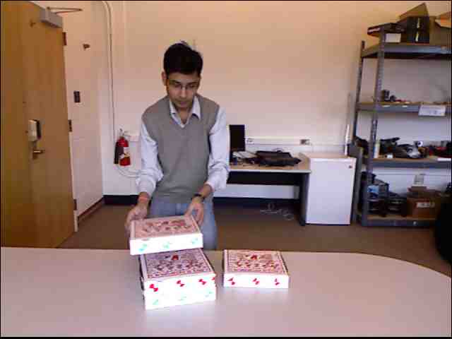
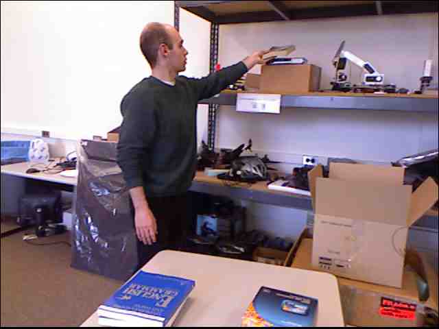
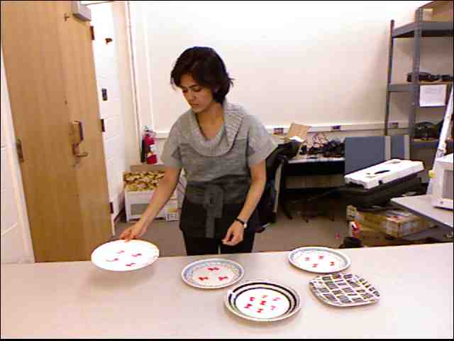
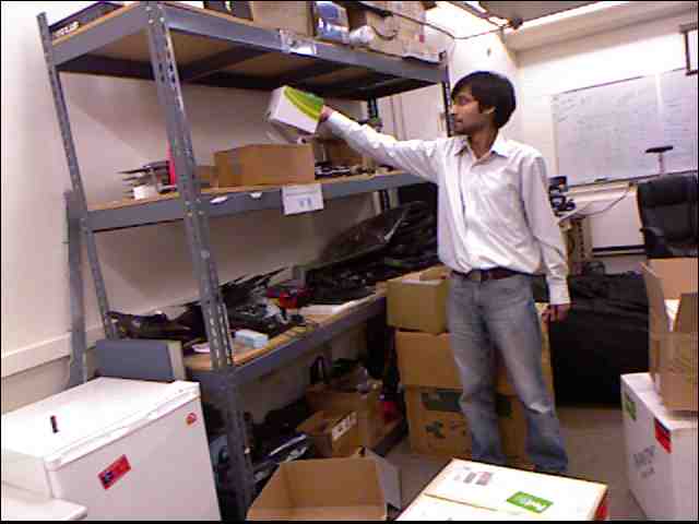
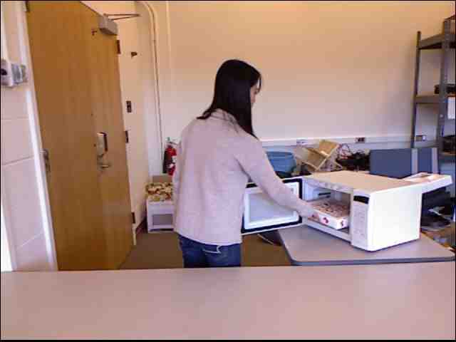
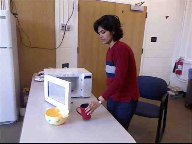
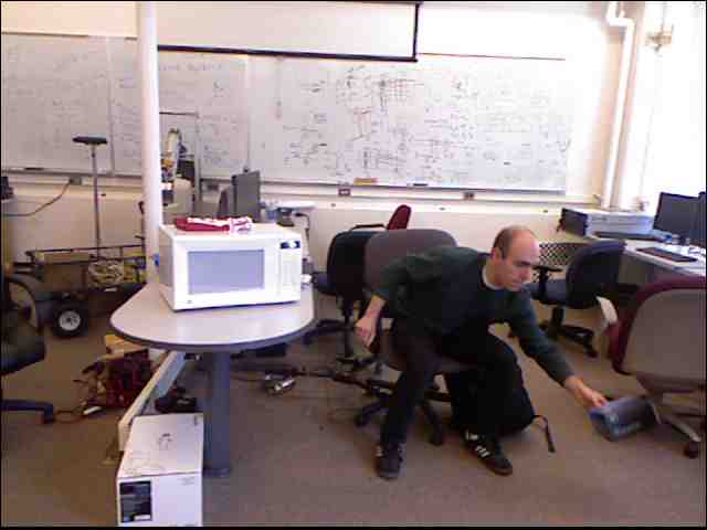
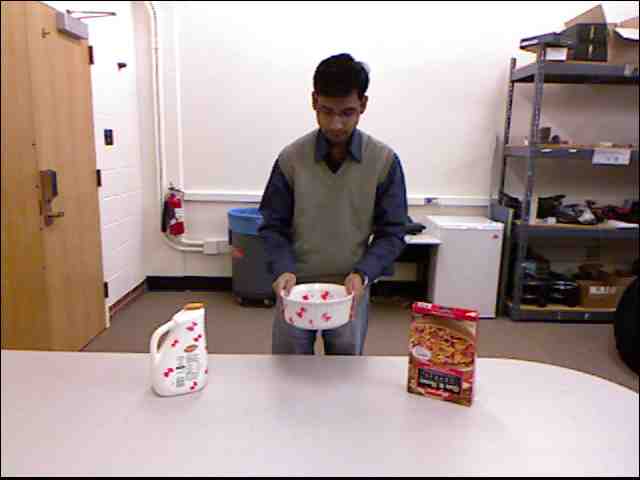
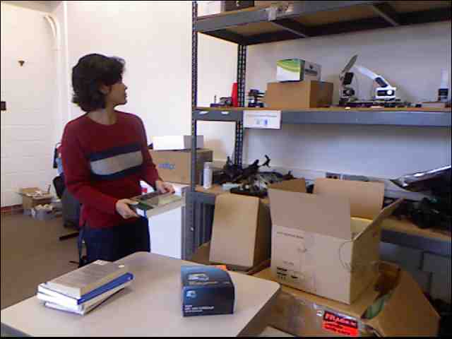
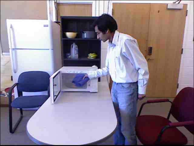
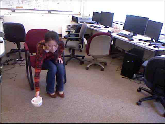
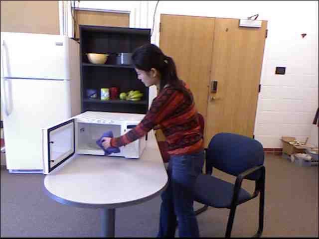
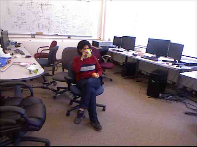
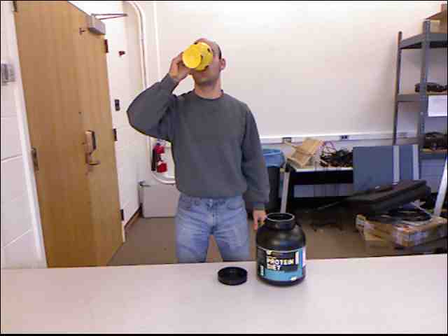
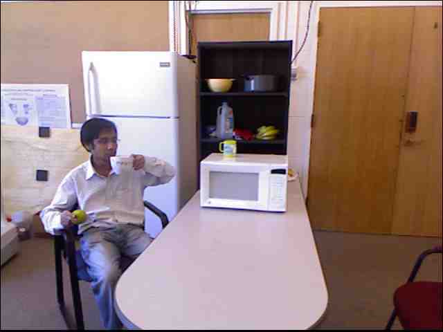
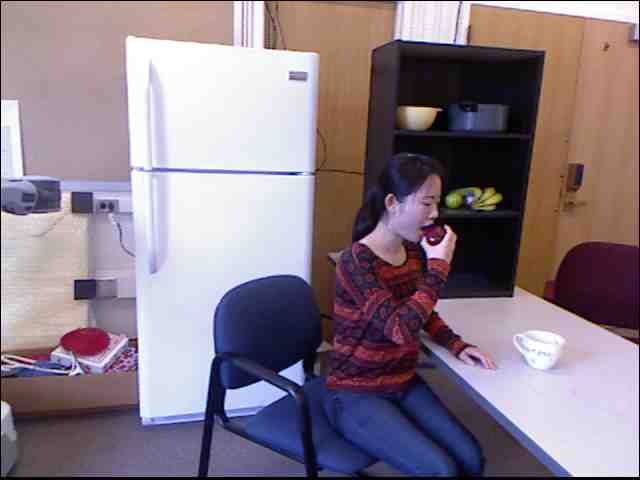
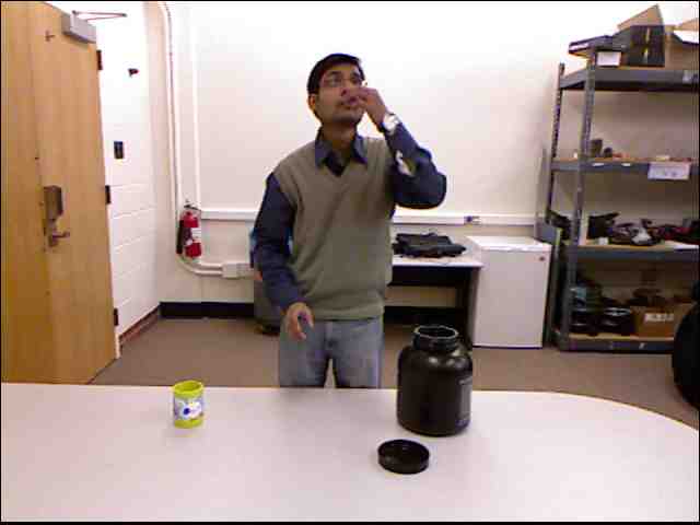
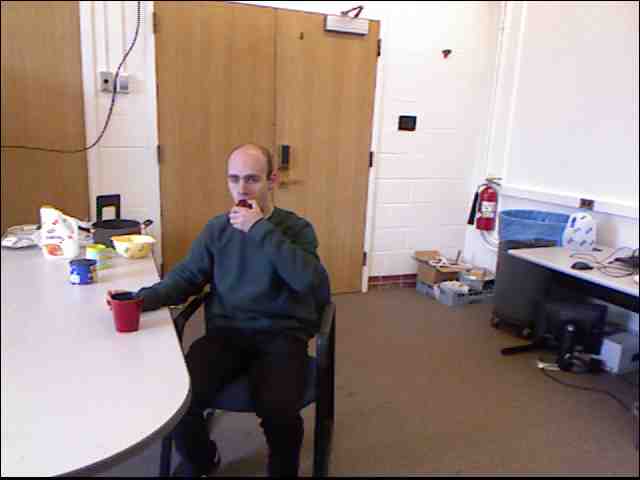
Figure 6: Example shots of reaching (first row), placing (second row), moving (third row), drinking (fourth row) and eating (fourth row) sub-activities from our dataset. There are significant variations in the way the subjects perform the sub-activity.

TABLE II: Description of high-level activities in terms of sub-activities. Note that some activities consist of same sub-activities but are executed in different order. The high-level activities (rows) are learnt using the algorithm in Section VIII-D and the sub-activities (columns) are learnt using the algorithm in Section VIII-B.

	reaching	moving	placing	opening	closing	eating	drinking	pouring	scrubbing	null
Making Cereal	✓	✓	✓					✓		✓
Taking Medicine	✓	✓	✓	✓		✓	✓			✓
Stacking Objects	✓	✓	✓							✓
Unstacking Objects	✓	✓	✓							✓
Microwaving Food	✓	✓	✓	✓	✓					✓
Picking Objects	✓	✓								✓
Cleaning Objects	✓	✓		✓	✓				✓	✓
Taking Food	✓		✓	✓	✓					✓
Arranging Objects	✓	✓	✓							✓
Having a Meal	✓	✓				✓	✓			✓

VIII-C Multiple Segmentations

Segmenting an RGB-D video in time can be noisy, and multiple segmentations may be valid. Therefore, we perform multiple segmentations by using different methods and criterion of segmentation (see Section VI for details). Thus, we get a set $\mathcal{H}$ of multiple segmentations, and let $h_{n}$ be the $n^{th}$ segmentation. A discriminant function ${E_{{\mathbf{w}^{h_{n}}}}({\mathbf{x}^{h_{n}}},{\mathbf{y}^{h_{n}}})}$ can now be defined for each $h_{n}$ as in Eq. (9). We now define a score function ${g_{\theta}({\mathbf{y}^{h_{n}}},{\mathbf{y}})}$ which gives a score for assigning the labels of the segments from ${\mathbf{y}^{h_{n}}}$ to ${\mathbf{y}}$,

$${g_{\theta_{n}}({\mathbf{y}^{h_{n}}},{\mathbf{y}})}=\sum_{k\in K}\sum_{i\in\mathcal{V}}\theta_{n}^{k}\mathbf{y}^{h_{n}k}_{i}{\mathbf{y}}_{i}^{k}$$ (17)

where $K=K_{o}\cup K_{a}$. Here, $\mathbf{\theta}_{n}^{k}$ can be interpreted as the confidence of labeling the segments of label $k$ correctly in the $n^{th}$ segmentation hypothesis. We want to find the labeling that maximizes the assignment score across all the segmentations. Therefore we can write inference in terms of a joint objective function as follows

$$\hat{{\mathbf{y}}}=\operatorname*{argmax}_{\mathbf{y}}\max_{{\mathbf{y}^{h_{n}}}\forall h_{n}\in\mathcal{H}}\sum_{h_{n}\in\mathcal{H}}[{E_{{\mathbf{w}^{h_{n}}}}({\mathbf{x}^{h_{n}}},{\mathbf{y}^{h_{n}}})}+{g_{\theta_{n}}({\mathbf{y}^{h_{n}}},{\mathbf{y}})}]$$ (18)

This formulation is equivalent to considering the labelings $y^{h_{n}}$ over the segmentations as unobserved variables. It is possible to use the latent structural SVM (Yu and Joachims,, 2009) to solve this, but it becomes intractable if the size of the segmentation hypothesis space is large. Therefore we propose an approximate two-step learning procedure to address this. For a given set of segmentations $\mathcal{H}$, we first learn the parameters ${\mathbf{w}^{h_{n}}}$ independently as described in Section IV. We then train the parameters $\mathbf{\theta}$ on a separate held-out training dataset. This can now be formulated as a QP

$$\min_{\theta} \frac{1}{2}\theta^{T}\theta-\sum_{h_{n}\in\mathbf{H}}{g_{\theta_{n}}({\mathbf{y}^{h_{n}}},{\mathbf{y}})}$$ (19)

$$s.t. \forall k\in K:\sum_{n=1}^{|\mathbf{H}|}\theta_{n}^{k}=1$$ (20)

Using the fact that the objective function defined in Eq. (18) is convex, we design an iterative two-step procedure where we solve for ${\mathbf{y}^{h_{n}}},\forall h_{n}\in\mathbf{H}$ in parallel and then solve for ${\mathbf{y}}$. This method is guaranteed to converge, and when the number of variables scales linearly with the number of segmentation hypothesis considered, the original problem in Eq. (18) will become considerably slow, but our method will still scale. More formally, we iterate between the following two problems:

$${\mathbf{\hat{y}}^{h_{n}}} = \operatorname*{argmax}_{\mathbf{y}^{h_{n}}}{E_{{\mathbf{w}^{h_{n}}}}({\mathbf{x}^{h_{n}}},{\mathbf{y}^{h_{n}}})}+{g_{\theta_{n}}({\mathbf{y}^{h_{n}}},\hat{{\mathbf{y}}})}\qquad$$ (21)

$$\hat{{\mathbf{y}}} = \operatorname*{argmax}_{\mathbf{y}}{g_{\theta_{n}}({\mathbf{\hat{y}}^{h_{n}}},{\mathbf{y}})}$$ (22)

VIII-D High-level Activity Classification.

For classifying the high-level activity, we compute the histograms of sub-activity and affordance labels and use them as features. However, some high-level activities, such as stacking objects and unstacking objects, have the same sub-activity and affordance sequences. Occlusion of objects plays a major role in being able to differentiate such activities. Therefore, we compute additional occlusion features by dividing the video into $n$ uniform length segments and finding the fraction of objects that are occluded fully or partially in the temporal segments. We then train a multi-class SVM classifier on training data using these features.

IX Experiments

IX-A Data

We test our model on two 3D activity datasets: Cornell Activity Dataset - 60 (CAD-60, Sung et al.,, 2012) and one that we collected. The CAD-60 dataset has 60 RGB-D videos of four different subjects performing 12 high-level activity classes. However, some of these activity classes contain only one sub-activity (e.g. working on a computer, cooking (stirring), etc.) and do not contain object interactions (e.g. talking on couch, relaxing on couch).

We collected the CAD-120 dataset (available at: http://pr.cs.cornell.edu/humanactivities, along with the code), which contains 120 activity sequences of ten different high-level activities performed by four different subjects, where each high-level activity was performed three times. We thus have a total of 61,585 RGB-D video frames in our dataset. The high-level activities are {making cereal, taking medicine, stacking objects, unstacking objects, microwaving food, picking objects, cleaning objects, taking food, arranging objects, having a meal}. The subjects were only given a high-level description of the task, and were asked to perform the activities multiple times with different objects. For example, the stacking and unstacking activities were performed with pizza boxes, plates and bowls. They performed the activities through a long sequence of sub-activities, which varied from subject to subject significantly in terms of length of the sub-activities, order of the sub-activities as well as in the way they executed the task. Table II specifies the set of sub-activities involved in each high-level activity. The camera was mounted so that the subject was in view (although the subject may not be facing the camera), but often there were significant occlusions of the body parts. See Fig. 2 and Fig. 6 for some examples.

We labeled our CAD-120 dataset with the sub-activity and the object affordance labels. Specifically, our sub-activity labels are {reaching, moving, pouring, eating, drinking, opening, placing, closing, scrubbing, null} and our affordance labels are {reachable, movable, pourable, pourto, containable, drinkable, openable, placeable, closable, scrubbable, scrubber, stationary}.

IX-B Object Tracking Results

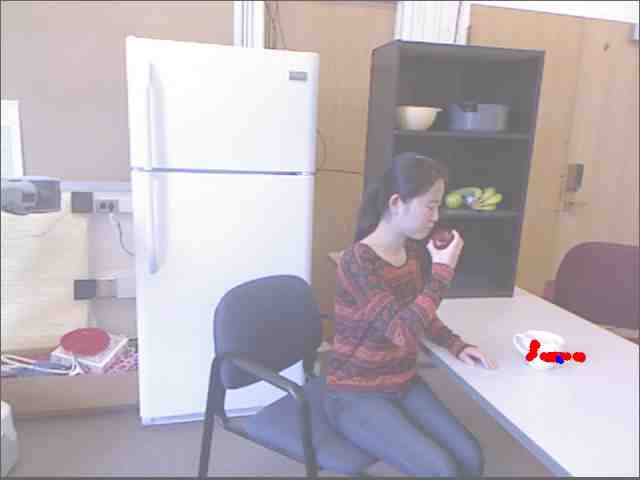
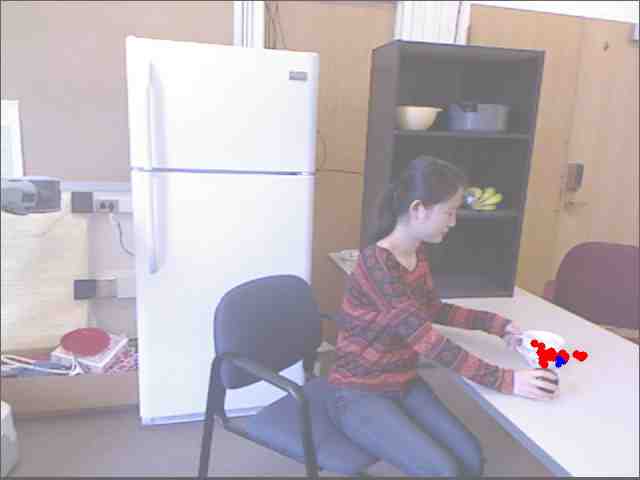
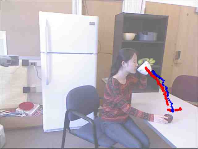
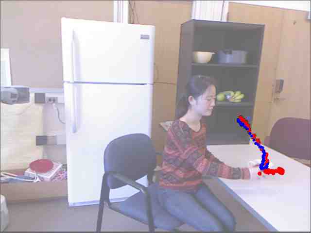
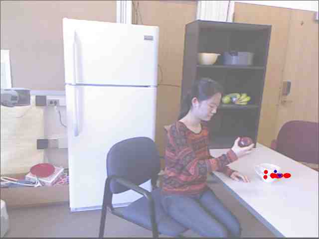
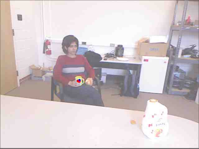
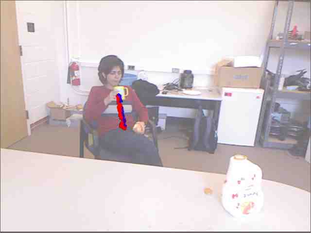
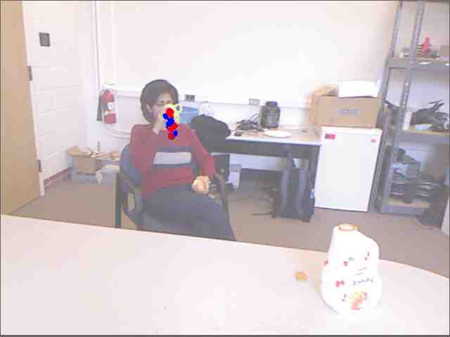
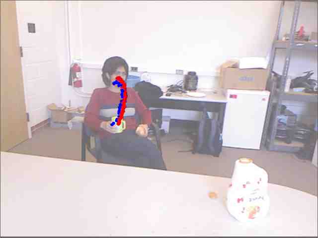
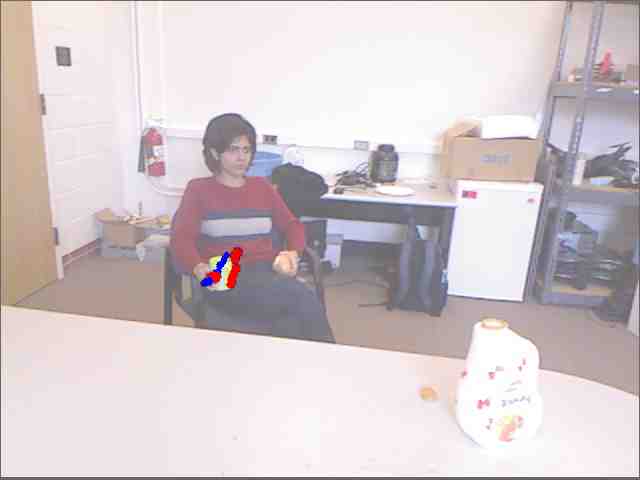
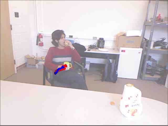
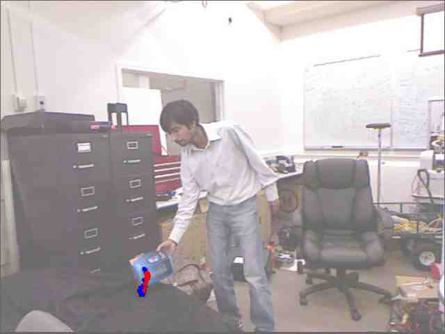
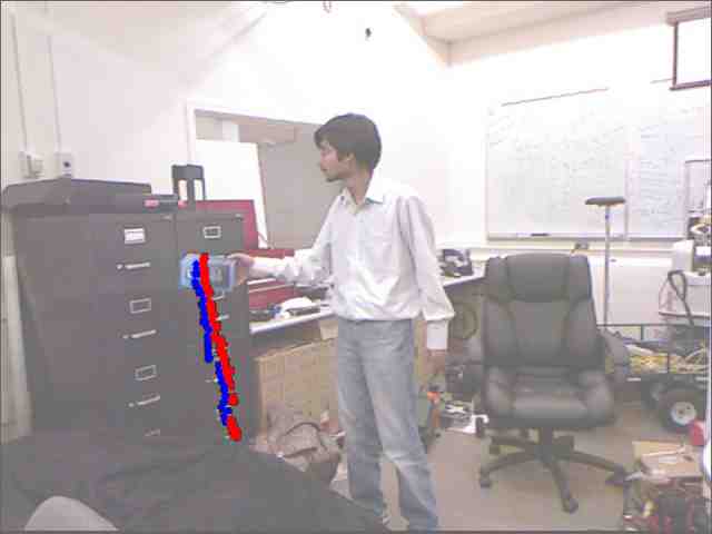
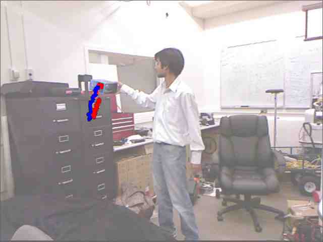
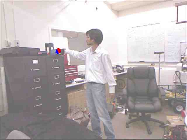
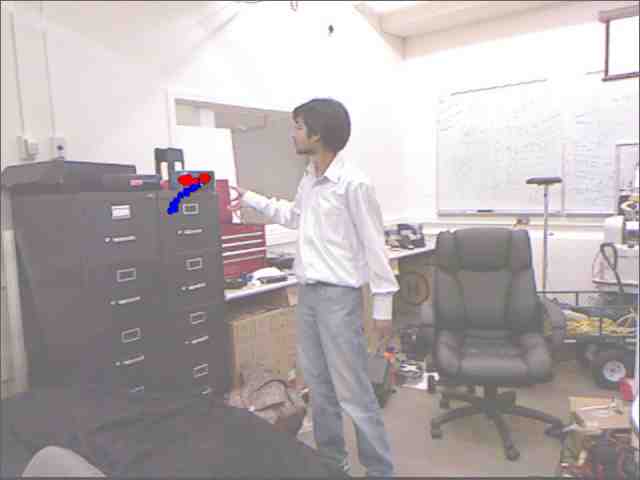
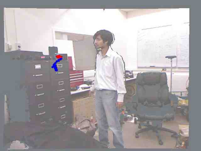
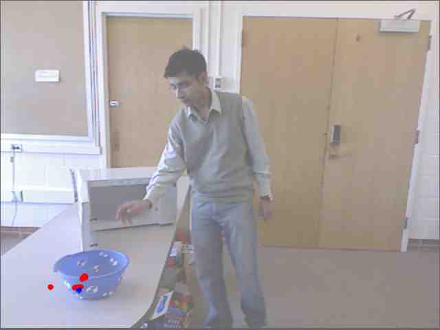
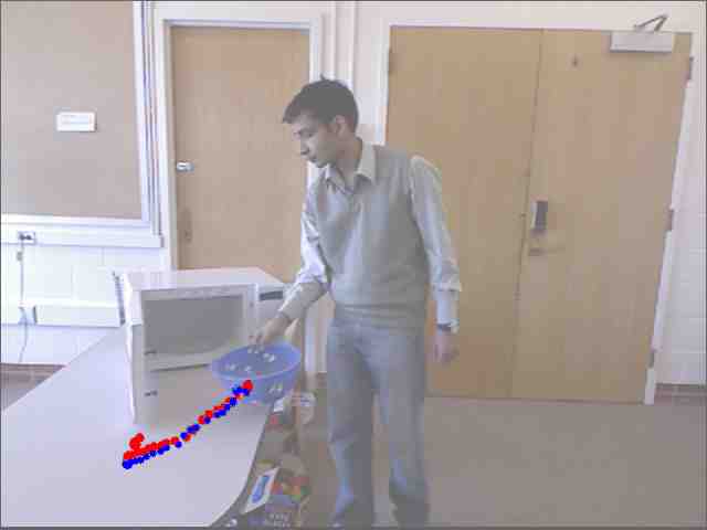
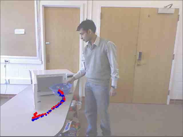
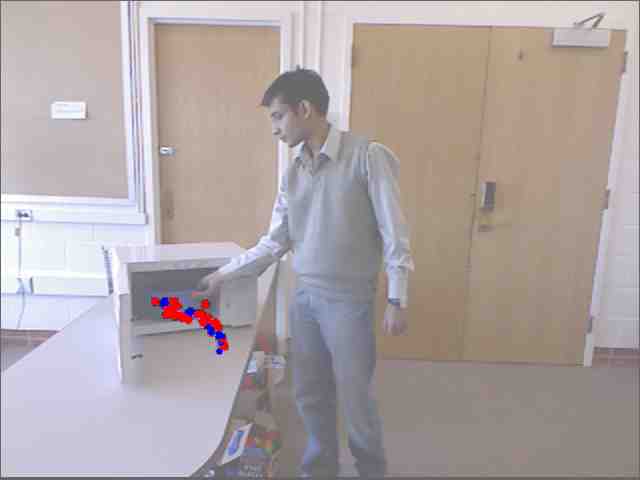
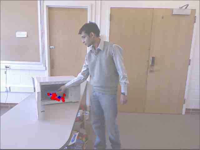
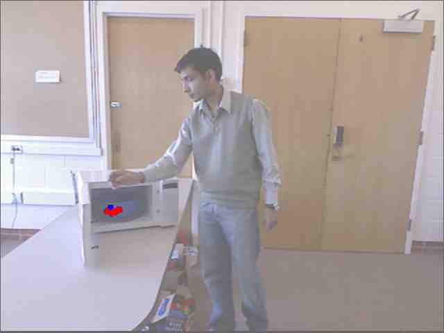
Figure 7: Tracking Results: Blue dots represent the trajectory of the center of tracked bounding box and red dots represent the trajectory of the center of ground-truth bounding box. (Best viewed in color.)

In order to evaluate our object detection and tracking method, we have generated the ground-truth bounding boxes of the objects involved in the activities. We do this by manually labeling the object bounding boxes in the images corresponding to every $50^{th}$ frame. We compute the bounding boxes in the rest of the frames by tracking using SIFT feature matching (Pele and Werman,, 2008), while enforcing depth consistency across the time frames for obtaining reliable object tracks.

Fig. 7 shows the visual output of our tracking algorithm. The center of the bounding box for each frame of the output is marked with a blue dot and that of the ground-truth is marked with a red dot. We compute the overlap of the bounding boxes obtained from our tracking method with the generated ground-truth bounding boxes. Table III shows the percentage overlap with the ground-truth when considering tracking from the given bounding box in the first frame both with and without object detections. As can be seen from Table III, our tracking algorithm produces greater than 10% overlap with the ground truth bounding boxes for 77.8% of the frames. Since, we only require that an approximate bounding box of the objects are given, 10% overlap is sufficient. We study the effect of the errors in tracking on the performance of our algorithm in Section IX-D.

TABLE III: Object Tracking Results, showing the % of frames which have $\geq$40%, $\geq$20% and $\geq$10% overlap with the ground-truth object bounding boxes.

	$\geq$40%	$\geq$20%	$\geq$10%
tracking w/o detection	49.2	65.7	75
tracking + detection	53.5	69.4	77.8

TABLE IV: Results on Cornell Activity Dataset (Sung et al.,, 2012), tested on “New Person” data for 12 activity classes.

	bathroom		bedroom		kitchen		living room		office		Average
	prec. (%)	rec. (%)	prec. (%)	rec. (%)	prec. (%)	rec. (%)	prec. (%)	rec. (%)	prec. (%)	rec. (%)	prec. (%)	rec. (%)
Sung et al., (2012)	72.7	65.0	76.1	59.2	64.4	47.9	52.6	45.7	73.8	59.8	67.9	55.5
Our method	88.9	61.1	73.0	66.7	96.4	85.4	69.2	68.7	76.7	75.0	80.8	71.4

IX-C Labeling results on the Cornell Activity Dataset 60 (CAD-60)

Table IV shows the precision and recall of the high-level activities on the CAD-60 dataset (Sung et al.,, 2012). Following Sung et al.’s (2012) experiments, we considered the same five groups of activities based on their location, and learnt a separate model for each location. To make it a fair comparison, we do not assume perfect segmentation of sub-activities and do not use any object information. Therefore, we train our model with only sub-activity nodes and consider segments of uniform size (20 frames per segments). We consider only a subset of our features described in Section IV that are possible to compute from the tracked human skeleton and RGB-D data provided in this dataset. Table IV shows that our model significantly outperforms Sung et al.’s MEMM model even when using only the sub-activity nodes and a simple segmentation algorithm.

TABLE V: Results on our CAD-120 dataset, showing average micro precision/recall, and average macro precision and recall for affordance, sub-activities and high-level activities. Standard error is also reported.

Full model, assuming ground-truth temporal segmentation is given.
	Object Affordance			Sub-activity			High-level Activity
	micro	macro		micro	macro		micro	macro
method	$P/R$ (%)	Prec. (%)	Recall (%)	$P/R$ (%)	Prec. (%)	Recall (%)	P/R (%)	Prec. (%)	Recall (%)
max class	65.7 $\pm$ 1.0	65.7 $\pm$ 1.0	8.3 $\pm$ 0.0	29.2 $\pm$ 0.2	29.2 $\pm$ 0.2	10.0 $\pm$ 0.0	10.0 $\pm$ 0.0	10.0 $\pm$ 0.0	10.0 $\pm$ 0.0
image only	74.2 $\pm$ 0.7	15.9 $\pm$ 2.7	16.0 $\pm$ 2.5	56.2 $\pm$ 0.4	39.6 $\pm$ 0.5	41.0 $\pm$ 0.6	34.7 $\pm$ 2.9	24.2 $\pm$ 1.5	35.8 $\pm$ 2.2
SVM multiclass	75.6 $\pm$ 1.8	40.6 $\pm$ 2.4	37.9 $\pm$ 2.0	58.0 $\pm$ 1.2	47.0 $\pm$ 0.6	41.6 $\pm$ 2.6	30.6 $\pm$ 3.5	27.4 $\pm$ 3.6	31.2 $\pm$ 3.7
MEMM (Sung et al.,, 2012)	-	-	-	-	-	-	26.4 $\pm$ 2.0	23.7 $\pm$ 1.0	23.7 $\pm$ 1.0
object only	86.9 $\pm$ 1.0	72.7 $\pm$ 3.8	63.1 $\pm$ 4.3	-	-	-	59.7 $\pm$ 1.8	56.3 $\pm$ 2.2	58.3 $\pm$ 1.9
sub-activity only	-	-	-	71.9 $\pm$ 0.8	60.9 $\pm$ 2.2	51.9 $\pm$ 0.9	27.4 $\pm$ 5.2	31.8 $\pm$ 6.3	27.7 $\pm$ 5.3
no temporal interactions	87.0 $\pm$ 0.8	79.8 $\pm$ 3.6	66.1 $\pm$ 1.5	76.0 $\pm$ 0.6	74.5 $\pm$ 3.5	66.7 $\pm$ 1.4	81.4 $\pm$ 1.3	83.2 $\pm$ 1.2	80.8 $\pm$ 1.4
no object interactions	88.4 $\pm$ 0.9	75.5 $\pm$ 3.7	63.3 $\pm$ 3.4	85.3 $\pm$ 1.0	79.6 $\pm$ 2.4	74.6 $\pm$ 2.8	80.6 $\pm$ 2.6	81.9 $\pm$ 2.2	80.0 $\pm$ 2.6
full model	91.8 $\pm$ 0.4	90.4 $\pm$ 2.5	74.2 $\pm$ 3.1	86.0 $\pm$ 0.9	84.2 $\pm$ 1.3	76.9 $\pm$ 2.6	84.7 $\pm$ 2.4	85.3 $\pm$ 2.0	84.2 $\pm$ 2.5
full model with tracking	88.2 $\pm$ 0.6	74.5 $\pm$ 4.3	64.9 $\pm$ 3.5	82.5 $\pm$ 1.4	72.9 $\pm$ 1.2	70.5 $\pm$ 3.0	79.0 $\pm$ 4.7	78.6 $\pm$ 4.1	78.3 $\pm$ 4.9
Full model, without assuming any ground-truth temporal segmentation is given.
full, 1 segment. (best)	83.1 $\pm$ 1.1	70.1 $\pm$ 2.3	63.9 $\pm$ 4.4	66.6 $\pm$ 0.7	62.0 $\pm$ 2.2	60.8 $\pm$ 4.5	77.5 $\pm$ 4.1	80.1 $\pm$ 3.9	76.7 $\pm$ 4.2
full, 1 segment. (averaged)	81.3 $\pm$ 0.4	67.8 $\pm$ 1.1	60.0 $\pm$ 0.8	64.3 $\pm$ 0.7	63.8 $\pm$ 1.1	59.1 $\pm$ 0.5	79.0 $\pm$ 0.9	81.1 $\pm$ 0.8	78.3 $\pm$ 0.9
full, multi-seg learning	83.9 $\pm$ 1.5	75.9 $\pm$ 4.6	64.2 $\pm$ 4.0	68.2 $\pm$ 0.3	71.1 $\pm$ 1.9	62.2 $\pm$ 4.1	80.6 $\pm$ 1.1	81.8 $\pm$ 2.2	80.0 $\pm$ 1.2
full, multi-seg learning + tracking	79.4 $\pm$ 0.8	62.5 $\pm$ 5.4	50.2 $\pm$ 4.9	63.4 $\pm$ 1.6	65.3 $\pm$ 2.3	54.0 $\pm$ 4.6	75.0 $\pm$ 4.5	75.8 $\pm$ 4.4	74.2 $\pm$ 4.6

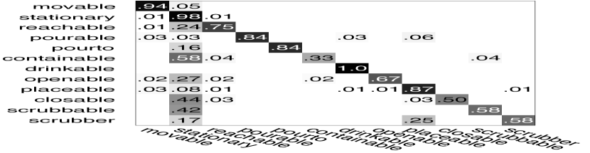
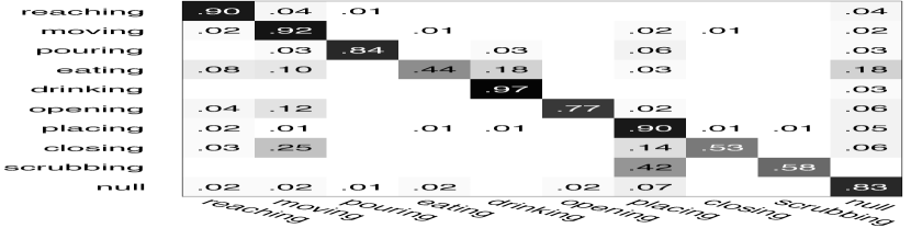
Figure 8: Confusion matrix for affordance labeling (left), sub-activity labeling (middle) and high-level activity labeling (right) of the test RGB-D videos.

IX-D Labeling results on the Cornell Activity Dataset 120 (CAD-120)

Table V shows the performance of various models on object affordance, sub-activity and high-level activity labeling. These results are obtained using 4-fold cross-validation and averaging performance across the folds. Each fold constitutes the activities performed by one subject, therefore the model is trained on activities of three subjects and tested on a new subject. We report both the micro and macro averaged precision and recall over various classes along with standard error. Since our algorithm can only predict one label for each segment, micro precision and recall are same as the percentage of correctly classified segments. Macro precision and recall are the averages of precision and recall respectively for all classes.

Assuming ground-truth temporal segmentation is given, the results for our full model are shown in Table V on line 10, its variations on lines 5–9 and the baselines on lines 1–4. The results in lines 11–14 correspond to the case when temporal segmentation is not assumed. In comparison to a basic SVM multiclass model (Joachims et al.,, 2009) (referred to as SVM multiclass when using all features and image only when using only image features), which is equivalent to only considering the nodes in our MRF without any edges, our model performs significantly better. We also compare with the high-level activity classification results obtained from the method presented in Sung et al., (2012). We ran their code on our dataset and obtain accuracy of 26.4%, whereas our method gives an accuracy of 84.7% when ground truth segmentation is available and 80.6% otherwise. Figure 9 shows a sequence of images from taking food activity along with the inferred labels. Figure 8 shows the confusion matrix for labeling affordances, sub-activities and high-level activities with our proposed method. We can see that there is a strong diagonal with a few errors such as scrubbing misclassified as placing, and picking objects misclassified as arranging objects.

We analyze our model to gain insight into which interactions provide useful information by comparing our full model to variants of our model.

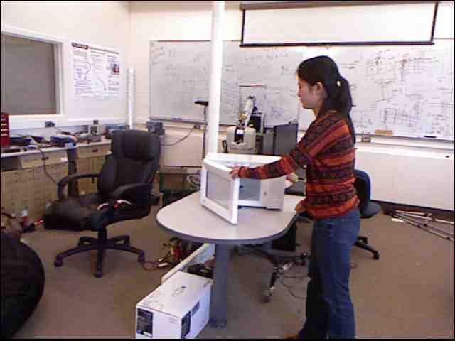
Subject opening openable object1

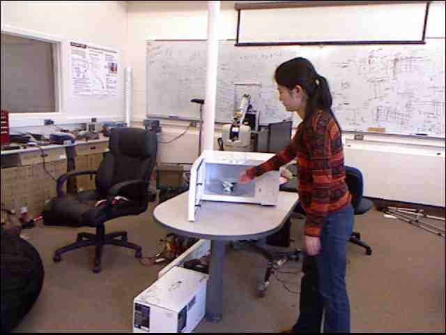
Subject reaching reachable object2

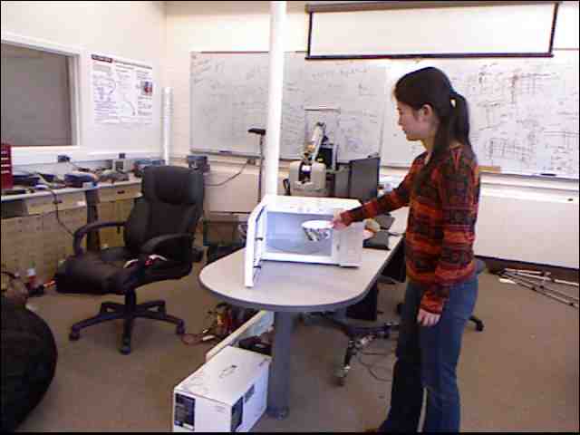
Subject moving movable object2

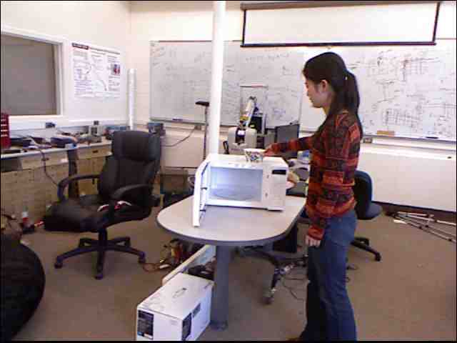
Subject placing placable object2

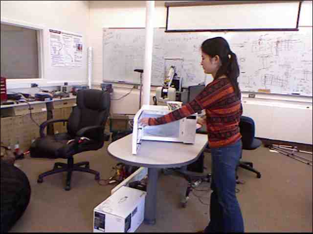
Subject reaching reachable object1

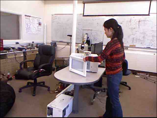
Subject closing closable object1

Subject moving movable object1

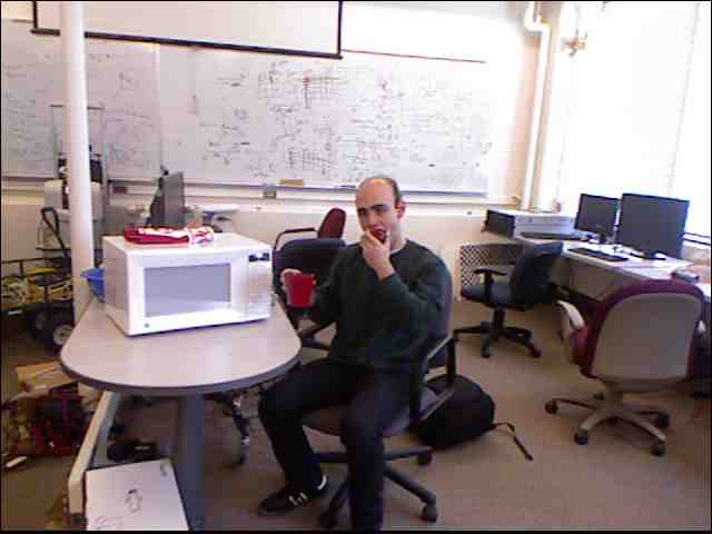
Subject eating

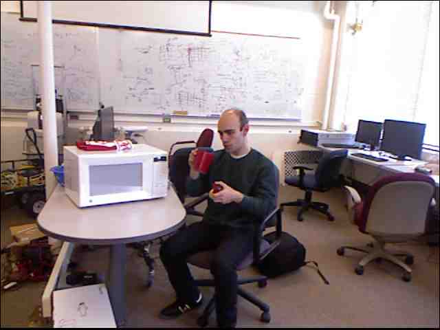
Subject moving movable object1

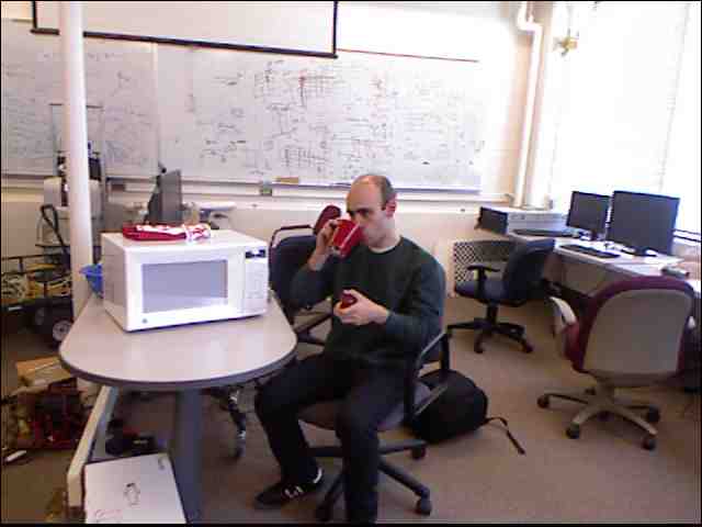
Subject drinking from drinkable object1

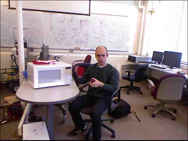
Subject moving movable object1

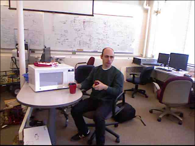
Subject placing placeable object1

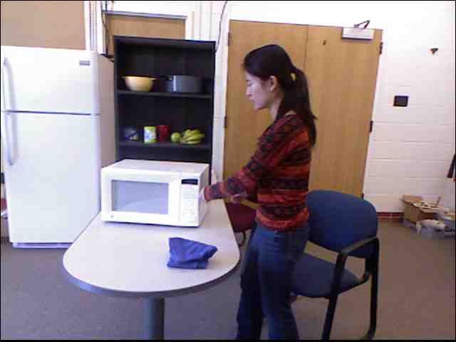
Subject reaching reachable object1

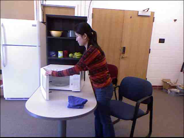
Subject opening openable object1

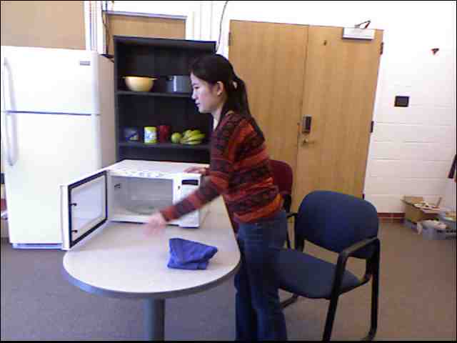
Subject reaching

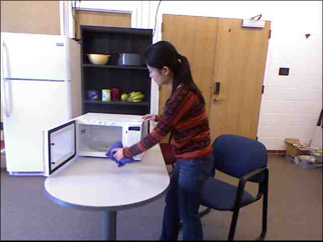
Subject moving movable object2

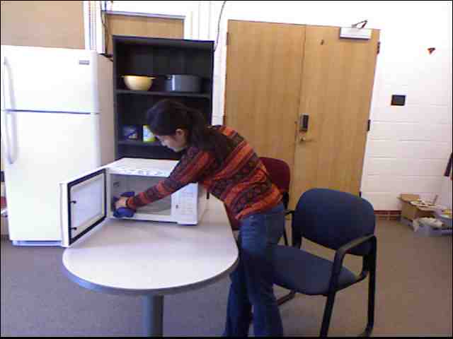
Subject scrubbing scrubbable object1 with scrubber object2

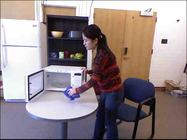
Subject moving movable object2

Figure 9: Descriptive output of our algorithm: Sequence of images from the taking food (Top Row), having meal (Middle Row) and cleaning objects (Bottom Row) activities labeled with sub-activity and object affordance labels. A single frame is sampled from the temporal segment to represent it.

How important is object context for activity detection? We show the importance of object context for sub-activity labeling by learning a variant of our model without the object nodes (referred to as sub-activity only). With object context, the micro precision increased by 14.1% and both macro precision and recall increased by around 23.3% over sub-activity only. Considering object information (affordance labels and occlusions) also improved the high-level activity accuracy by three-fold.

How important is activity context for affordance detection? We also show the importance of context from sub-activity for affordance detection by learning our model without the sub-activity nodes (referred to as object only). With sub-activity context, the micro precision increased by 4.9% and the macro precision and recall increased by 17.7% and 11.1% respectively for affordance labeling over object only. The relative gain is less compared with that obtained in sub-activity detection as the object only model still has object–object context which helps in affordance detection.

How important is object–object context for affordance detection? In order to study the effect of the object–object interactions for affordance detection, we learnt our model without the object-object edge potentials (referred to as no object interactions). We see a considerable improvement in affordance detection when the object interactions are modeled, the macro recall increased by 14.9% and the macro precision by about 10.9%. This shows that sometimes just the context from the human activity alone is not sufficient to determine the affordance of an object.

How important is temporal context? We also learn our model without the temporal edges (referred to as no temporal interactions). Modeling temporal interactions increased the micro precision by 4.8% and 10.0% for affordances and sub-activities respectively and increased the micro precision for high-level activity by 3.3%.

How important is reliable human pose detection? In order understand the effect of the errors in human pose tracking, we consider the affordances that require direct contact by human hands, such as movable, openable, closable, drinkable, etc. The distance of the predicted hand locations to the object should be zero at the time of contact. We found that for the correct predictions, these distances had a mean of 3.8 cm and variance of 48.1 cm. However, for the incorrect predictions, these distances had a mean that was 43.3% higher and a variance that was 53.8% higher. This indicates that the prediction accuracies can potentially be improved with more robust human pose tracking.

How important is reliable object tracking? We show the effect of having reliable object tracking by comparing to the results obtained from using our object tracking algorithm mentioned in Section V. We see that using the object tracks generated by our algorithm gives slightly lower micro precision/recall values compared with using ground-truth object tracks, around 3.5% drop in affordance and sub-activity detection, and 5.7% drop in high-level activity detection. The drop in macro precision and recall are higher, which shows that the performance of few classes are effected more than the others. In future work, one can increase accuracy by improving object tracking.

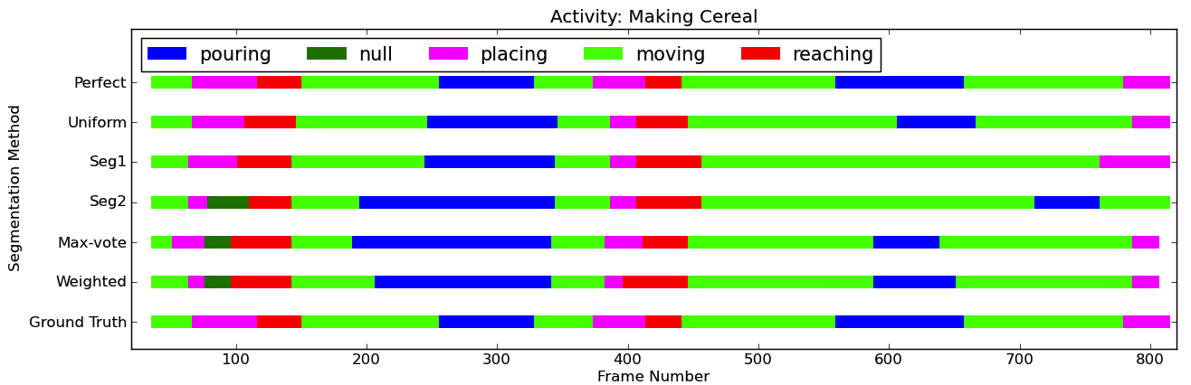
Figure 10: Comparison of the sub-activity labeling of various segmentations. This activity involves the sub-activities: reaching, moving, pouring and placing as colored in red, green, blue and magenta respectively. The x-axis denotes the time axis numbered with frame numbers. It can be seen that the various individual segmentation labelings are not perfect and make different mistakes, but our method for merging these segmentations selects the correct label for many frames.

Results with multiple segmentations. Given the RGB-D video and initial bounding boxes for objects in the first frame, we obtain the final labeling using our method described in Section VIII-C. To generate the segmentation hypothesis set $\mathcal{H}$ we consider three different segmentation algorithms, and generate multiple segmentations by changing their parameters as described in Section VI. The lines 11–13 of Table V show the results of the best performing segmentation, average performance all the segmentations considered, and our proposed method for combining the segmentations respectively. We see that our method improves the performance over considering a single best performing segmentation: macro precision increased by 5.8% and 9.1% for affordance and sub-activity labeling respectively. Fig. 10 shows the comparison of the sub-activity labeling of various segmentations, our end-to-end labeling and the ground-truth labeling for one making cereal high-level activity video. It can be seen that the various individual segmentation labelings are not perfect and make different mistakes, but our method for merging these segmentations selects the correct label for many frames. Line 14 of Table V show the results of our proposed method for combining the segmentations along with using our object tracking algorithm. The numbers show a drop compared with the case of using ground-truth tracks, therefore providing a scope for improvement by using more reliable tracking algorithms.

IX-E Robotic Applications

We demonstrate the use of our learning algorithm in two robotics applications. First, we show that the knowledge of the activities currently being performed enables a robot to assist the human by performing an appropriate response action. Second, we show that the knowledge of the affordances of the objects enables a robot to use them appropriately when manipulating them.

We use Cornell’s Kodiak, a PR2 robot, in our experiments. Kodiak is mounted with a Microsoft Kinect, which is used as the main input sensor to obtain the RGB-D video stream. We used the OpenRAVE libraries (Diankov,, 2010) for programming the robot to perform the pre-programmed assistive tasks.

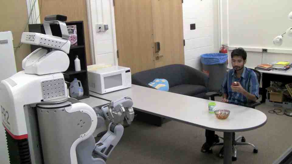
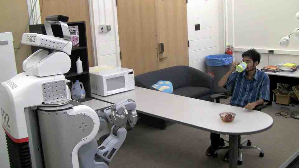
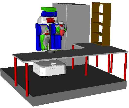
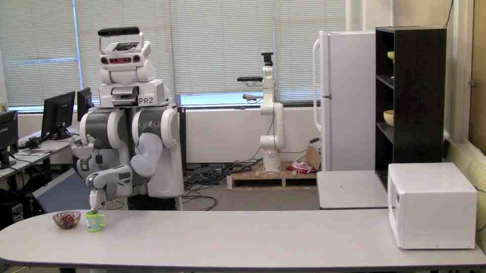
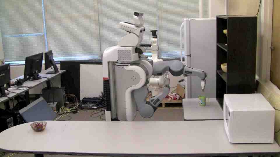
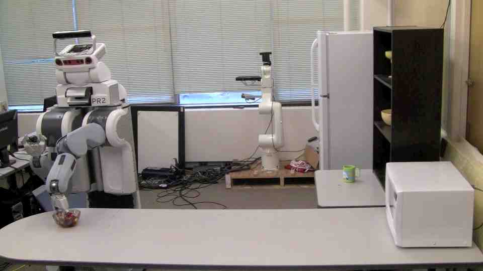
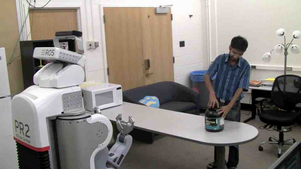
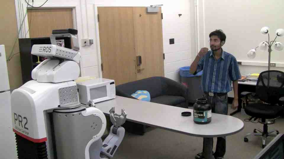
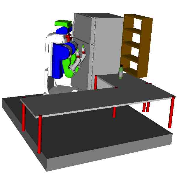
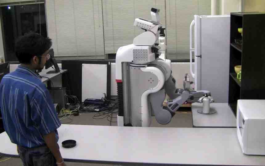
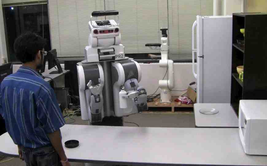
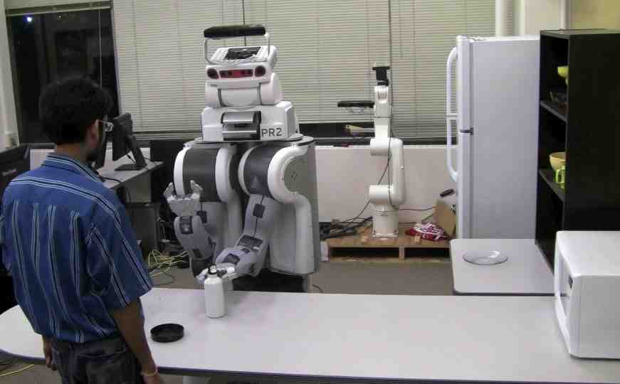
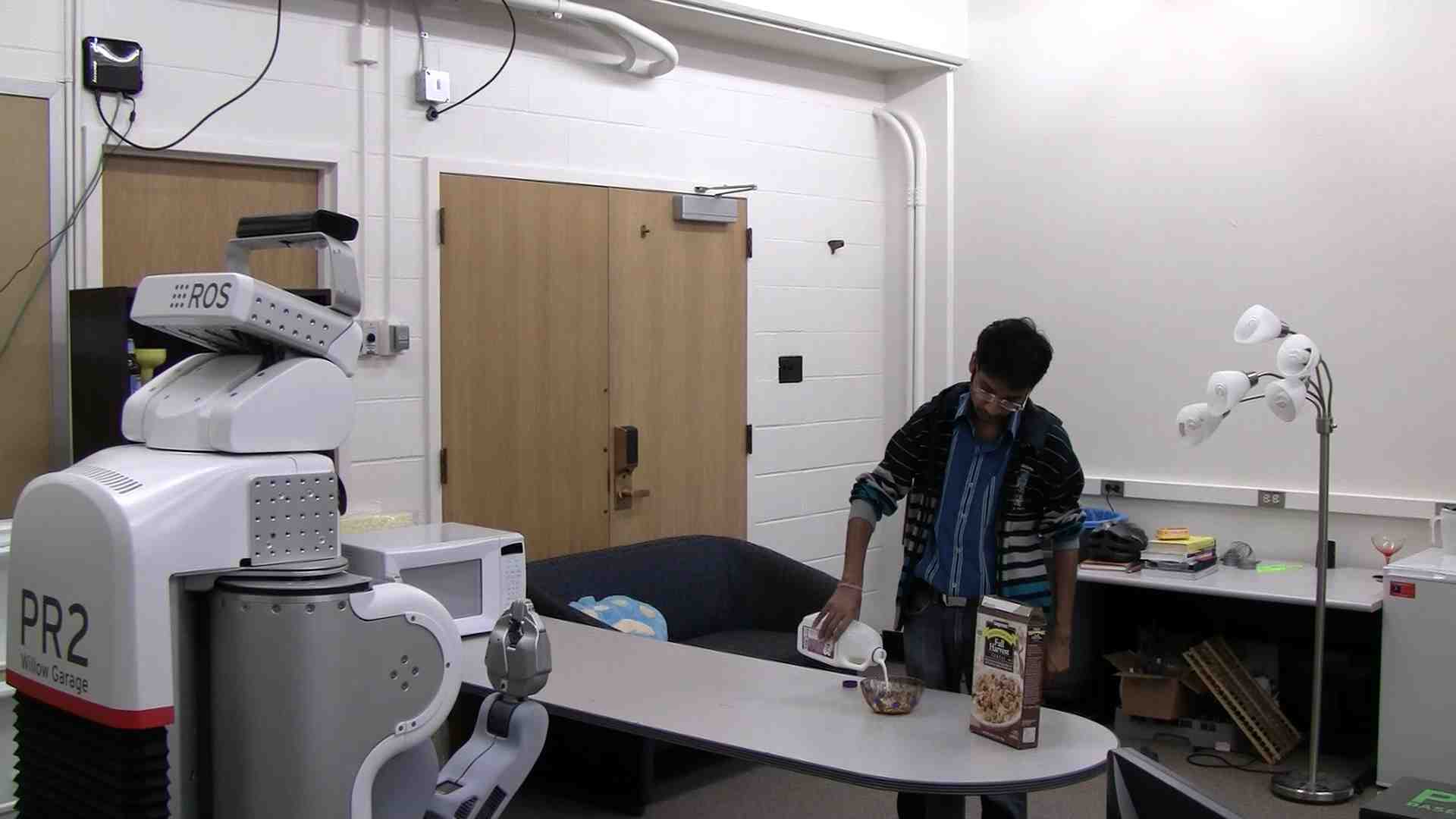
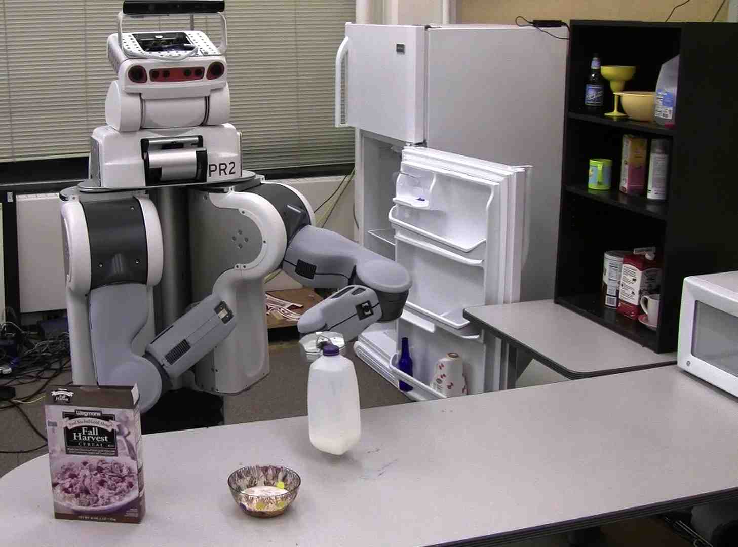
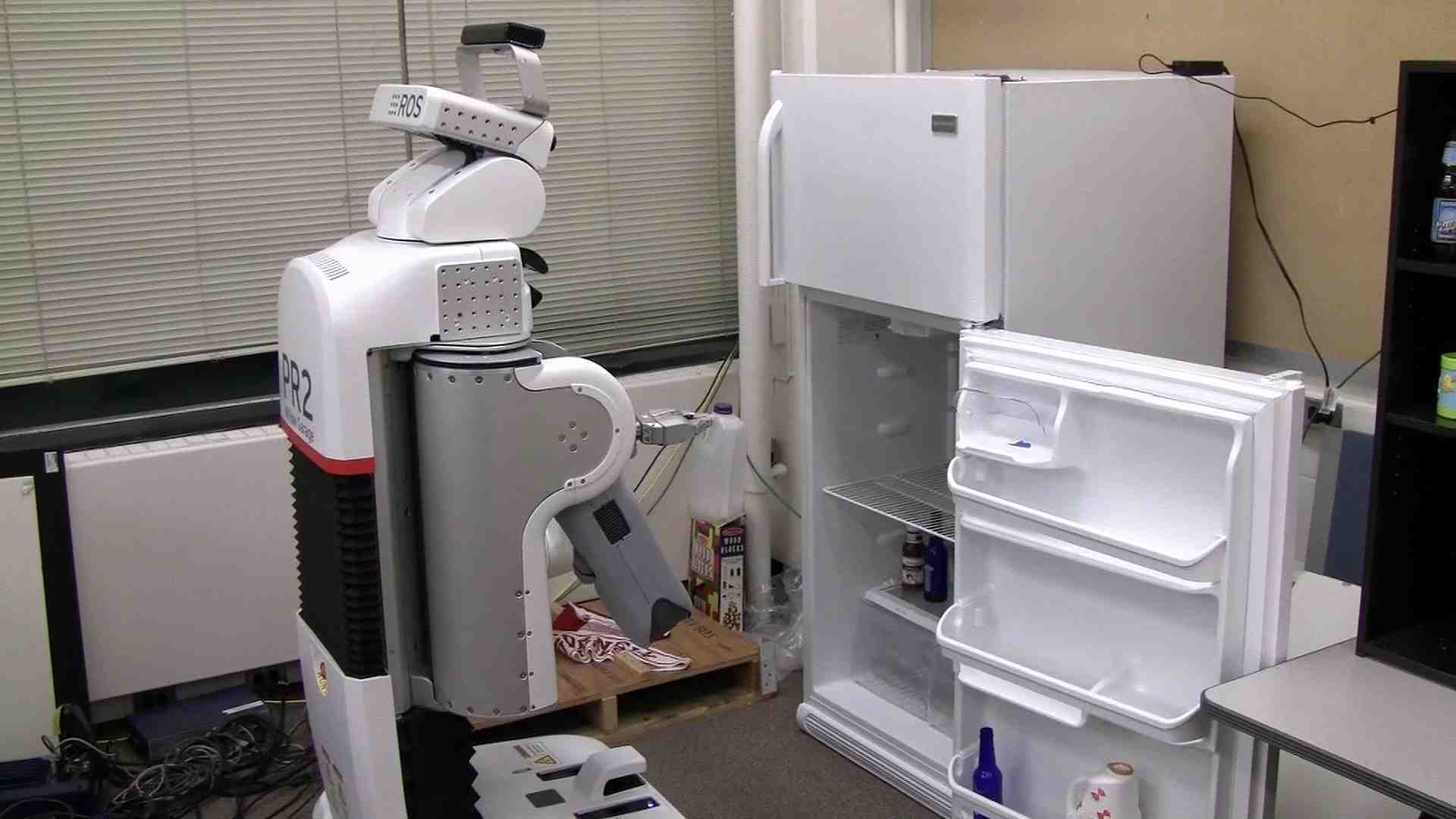
Figure 11: Robot performing the task of assisting humans: (top row) robot clearing the table after detecting having a meal activity, (middle row) robot fetching a bottle of water after detecting taking a medicine activity and (third row) robot putting milk in the fridge after detecting making cereal activity. First two columns show the robot observing the activity, third row shows the robot planning the response in simulation and the last three columns show the robot performing the response action.

Assisting Humans. There are several modes of operation for a robot performing assistive tasks. For example, the robot can perform some tasks completely autonomous, independent of the humans. For some other tasks, the robot needs to act more reactively. That is, depending on the task and current human activity taking place, perform a complementary sub-task. For example, bring a glass of water when a person is attempting to take medicine (and there is no glass within person’s reach). Such a behavior is possible only when the activities are successfully detected. In this experiment, we demonstrate that our algorithm for detecting the human activities enables a robot to take such (pre-programmed) reactive actions.

We consider the following three scenarios:

• Having Meal: The subject eats food from a bowl and drinks water from a cup in this activity. On detecting the having meal activity, the robot assists by clearing the table (i.e. move the cup and the bowl to another place) after the subject finishes eating.

• Taking Medicine: The subjects opens the medicine container, takes the medicine, and waits as there is no water nearby. The robot assists the subject by bringing a glass of water on detecting the taking medicine activity.

• Making Cereal: The subject prepares cereal by pouring cereal and milk in to a bowl. On detecting the activity, the robot responds by taking the milk and putting it into the refrigerator.

Our robot was placed in a kitchen environment so that it can observe the activity being performed by the subject. We found that our robot successfully detected the activities and performed the above described reactive actions. Fig. 11 shows the sequence of images of the robot detecting the activity being performed, planning the response in simulation and then performing the appropriate response for all three activities described above.

Using Affordances. An important component of our work is to learn affordances. In particular, by observing how the humans interact with the objects, a robot can figure out the affordances of the objects. Therefore, it can use these inferred affordances to interact with objects in a meaningful way. For example, given an instruction of ‘clear the table’, the robot should be able to perform the response in a desirable way: move the bowl with cereal without tilting it, and not move the microwave. In this experiment, we demonstrate that our algorithm for labeling the affordances explicitly helps in manipulation.

In our setting, we directly infer the object affordances (movable, pourable, drinkable, etc.). Therefore, we only need to encode the low-level control actions of each affordance, e.g. to move only movable objects, and to execute constrained movement, i.e. no rotation in the xy plane, for objects with affordances such as pour-to, pourable or drinkable, etc. The robot is allowed to observe various activities performed with the objects and it uses our learning algorithms to infer the affordances associated with the objects. When an instruction is given to the robot, such as ‘clear the table’ or ‘move object x’, it uses the inferred affordances to perform the response.

We demonstrate this in two scenarios for the task of ‘clearing the table’: detecting movable objects and detecting constrained movement. We consider a total of seven activities with nine unique objects. Some objects were used in multiple activities, with a total of 19 object instances. Two of these activities were other high-level activities that were not seen during training, but comprise sequences of the learned affordances and sub-activities. The results are summarized in Table VI.

TABLE VI: Robot Object Manipulation Results, showing the accuracy achieved by the Kodiak PR2 performing the two manipulation tasks, with and without multiple observations.

task	# instance	accuracy (%)	accuracy (%) (multi. obsrv.)
object movement	19	100	100
constrained movement	15	80	100

In the scenario of detecting movable objects, the robot was programmed to move only objects with inferred movable affordance, to a specified location. There were a total of 15 instances of movable objects. The robot was able to correctly identify all movable objects using our model and could perform the moving task with 100% accuracy.

In the scenario of constrained movement, i.e. the robot should not tilt the objects which contain food items or liquids when moving them. In order to achieve this, we have programmed the robot to perform constrained movement without tilting the objects if it has inferred at least one of the following affordances: {drinkable, pourable, pour-to}. The robot was able to correctly identify constraint movement for 80% of the movable instances. Also, if we let the robot observe the activities for a longer time, i.e. let the subject perform multiple activities with the objects and aggregate the affordances associated with the objects before performing the task, the robot is able to perform the task with 100% accuracy.

These experiments show that robot can use the affordances for manipulating the objects in a more meaningful way. Some affordances such as moving are easy to detect, where as some complicated affordances such as pouring might need more observations to be detected correctly. Also, by considering other high-level activities in addition to those used for learning, we have also demonstrated the generalizability of our algorithm for affordance detection.

We have made the videos of our results, along with the CAD-120 dataset and code, available at http://pr.cs.cornell.edu/humanactivities

X Conclusion and Discussion

In this paper, we have considered the task of jointly labeling human sub-activities and object affordances in order to obtain a descriptive labeling of the activities being performed in the RGB-D videos. The activities we consider happen over a long time period, and comprise several sub-activities performed in a sequence. We formulated this problem as a MRF, and learned the parameters of the model using a structural SVM formulation. Our model also incorporates the temporal segmentation problem by computing multiple segmentations and considering labeling over these segmentations as latent variables. In extensive experiments over a challenging dataset, we show that our method achieves an accuracy of 79.4% for affordance, 63.4% for sub-activity and 75.0% for high-level activity labeling on the activities performed by a different subject than those in the training set. We also showed that it is important to model the different properties (object affordances, object–object interaction, temporal interactions, etc.) in order to achieve good performance. We also demonstrate the use of our activity and affordance labeling by a PR2 robot in the task of assisting humans with their daily activities. We have shown that being able to infer affordance labels enables the robot to perform the tasks in a more meaningful way.

In this growing area of RGB-D activity recognition, we have presented algorithms for activity and affordance detection and also demonstrated their use in assistive robots, where our robot responds with pre-programmed actions. We have focused on the algorithms for temporal segmentation and labeling while using simple bounding-box detection and tracking algorithms. However, improvements to object perception and task-planning, while taking into consideration the human-robot interaction aspects, are needed for making assistive robots working efficiently alongside humans.

XI Acknowledgements

We thank Li Wang for his significant contributions to the robotic experiments. We also thank Yun Jiang, Jerry Yeh, Vaibhav Aggarwal, and Thorsten Joachims for useful discussions. This research was funded in part by ARO award W911NF-12-1-0267, and by Microsoft Faculty Fellowship and Alfred P. Sloan Research Fellowship to one of us (Saxena).

References

- Aggarwal and Ryoo, (2011) Aggarwal, J. K. and Ryoo, M. S. (2011). Human activity analysis: A review. ACM Comp Surveys (CSUR).
- Aksoy et al., (2010) Aksoy, E., Abramov, A., Worgotter, F., and Dellen, B. (2010). Categorizing object-action relations from semantic scene graphs. In ICRA.
- Aksoy et al., (2011) Aksoy, E. E., Abramov, A., Dörr, J., Ning, K., Dellen, B., and Wörgötter, F. (2011). Learning the semantics of object-action relations by observation. IJRR, 30(10):1229–1249.
- Aldoma et al., (2012) Aldoma, A., Tombari, F., and Vincze, M. (2012). Supervised learning of hidden and non-hidden 0-order affordances and detection in real scenes. In ICRA.
- Anand et al., (2012) Anand, A., Koppula, H. S., Joachims, T., and Saxena, A. (2012). Contextually guided semantic labeling and search for 3d point clouds. IJRR.
- Bollini et al., (2012) Bollini, M., Tellex, S., Thompson, T., Roy, N., and Rus, D. (2012). Interpreting and executing recipes with a cooking robot. In ISER.
- Choi and Christensen, (2012) Choi, C. and Christensen, H. I. (2012). Robust 3d visual tracking using particle filtering on the special euclidean group: A combined approach of keypoint and edge features. IJRR, 31(4):498–519.
- Collet et al., (2011) Collet, A., Martinez, M., and Srinivasa, S. S. (2011). The MOPED framework: Object Recognition and Pose Estimation for Manipulation. IJRR.
- Dalal and Triggs, (2005) Dalal, N. and Triggs, B. (2005). Histograms of oriented gradients for human detection. In CVPR.
- Diankov, (2010) Diankov, R. (2010). Automated Construction of Robotic Manipulation Programs. PhD thesis, Carnegie Mellon University, Robotics Institute.
- Felzenszwalb and Huttenlocher, (2004) Felzenszwalb, P. F. and Huttenlocher, D. (2004). Efficient graph-based image segmentation. IJCV, 59(2).
- Finley and Joachims, (2008) Finley, T. and Joachims, T. (2008). Training structural svms when exact inference is intractable. In ICML.
- Fox et al., (2011) Fox, E., Sudderth, E., Jordan, M., and Willsky, A. (2011). Bayesian Nonparametric Inference of Switching Dynamic Linear Models. IEEE Transactions on Signal Processing, 59(4).
- Gall et al., (2011) Gall, J., Fossati, A., and van Gool, L. (2011). Functional categorization of objects using real-time markerless motion capture. In CVPR.
- Gibson, (1979) Gibson, J. (1979). The Ecological Approach to Visual Perception. Houghton Mifflin.
- Gupta et al., (2009) Gupta, A., Kembhavi, A., and Davis, L. (2009). Observing human-object interactions: Using spatial and functional compatibility for recognition. IEEE T-PAMI, 31(10):1775–1789.
- Hammer et al., (1984) Hammer, P., Hansen, P., and Simeone, B. (1984). Roof duality, complementation and persistency in quadratic 0–1 optimization. Mathematical Prog., 28(2):121–155.
- Henry et al., (2012) Henry, P., Krainin, M., Herbst, E., Ren, X., and Fox, D. (2012). Rgb-d mapping: Using kinect-style depth cameras for dense 3d modeling of indoor environments. IJRR, 31(5):647–663.
- Hermans et al., (2011) Hermans, T., Rehg, J. M., and Bobick, A. (2011). Affordance prediction via learned object attributes. In ICRA: Workshop on Semantic Perception, Mapping, and Exploration.
- Hoai and De la Torre, (2012) Hoai, M. and De la Torre, F. (2012). Maximum margin temporal clustering. In Proceedings of International Conference on Artificial Intelligence and Statistics.
- Hoai et al., (2011) Hoai, M., Lan, Z., and De la Torre, F. (2011). Joint segmentation and classification of human actions in video. In CVPR.
- (22) Jiang, Y., Li, Z., and Chang, S. (2011a). Modeling scene and object contexts for human action retrieval with few examples. IEEE Trans Circuits & Sys Video Tech.
- (23) Jiang, Y., Lim, M., and Saxena, A. (2012a). Learning object arrangements in 3d scenes using human context. In ICML.
- (24) Jiang, Y., Lim, M., Zheng, C., and Saxena, A. (2012b). Learning to place new objects in a scene. IJRR.
- (25) Jiang, Y., Moseson, S., and Saxena, A. (2011b). Efficient grasping from rgbd images: Learning using a new rectangle representation. In ICRA.
- Jiang and Saxena, (2012) Jiang, Y. and Saxena, A. (2012). Hallucinating humans for learning robotic placement of objects. In ISER.
- Joachims et al., (2009) Joachims, T., Finley, T., and Yu, C. (2009). Cutting-plane training of structural SVMs. Mach. Learn., 77(1).
- Kjellström et al., (2011) Kjellström, H., Romero, J., and Kragic, D. (2011). Visual object-action recognition: Inferring object affordances from human demonstration. CVIU, 115(1):81–90.
- Koller and Friedman, (2009) Koller, D. and Friedman, N. (2009). Probabilistic Graphical Models: Principles and Techniques. MIT Press.
- Konidaris et al., (2012) Konidaris, G., Kuindersma, S., Grupen, R., and Barto, A. (2012). Robot learning from demonstration by constructing skill trees. IJRR, 31(3):360–375.
- Koppula et al., (2011) Koppula, H., Anand, A., Joachims, T., and Saxena, A. (2011). Semantic labeling of 3d point clouds for indoor scenes. In NIPS.
- Koppula et al., (2012) Koppula, H. S., Gupta, R., and Saxena, A. (2012). Human activity learning using object affordances from rgb-d videos. CoRR, abs/1208.0967.
- Kormushev et al., (2010) Kormushev, P., Calinon, S., and Caldwell, D. G. (2010). Robot motor skill coordination with EM-based reinforcement learning. In IROS.
- Krainin et al., (2011) Krainin, M., Henry, P., Ren, X., and Fox, D. (2011). Manipulator and object tracking for in-hand 3d object modeling. IJRR, 30(11):1311–1327.
- (35) Lai, K., Bo, L., Ren, X., and Fox, D. (2011a). A Large-Scale Hierarchical Multi-View RGB-D Object Dataset. In ICRA.
- (36) Lai, K., Bo, L., Ren, X., and Fox, D. (2011b). Sparse Distance Learning for Object Recognition Combining RGB and Depth Information. In ICRA.
- Laptev et al., (2008) Laptev, I., Marszalek, M., Schmid, C., and Rozenfeld, B. (2008). Learning realistic human actions from movies. In CVPR.
- Li et al., (2012) Li, C., Kowdle, A., Saxena, A., and Chen, T. (2012). Towards holistic scene understanding: Feedback enabled cascaded classification models. Pattern Analysis and Machine Intelligence, IEEE Transactions on, 34(7):1394–1408.
- Li et al., (2010) Li, W., Zhang, Z., and Liu, Z. (2010). Action recognition based on a bag of 3d points. In Workshop on CVPR for Human Communicative Behavior Analysis.
- Liu et al., (2009) Liu, J., Luo, J., and Shah, M. (2009). Recognizing realistic actions from videos “in the wild”. In CVPR.
- Lopes and Santos-Victor, (2005) Lopes, M. and Santos-Victor, J. (2005). Visual learning by imitation with motor representations. Systems, Man, and Cybernetics, Part B: Cybernetics, IEEE Transactions on, 35(3):438 –449.
- Matikainen et al., (2012) Matikainen, P., Sukthankar, R., and Hebert, M. (2012). Model recommendation for action recognition. In CVPR.
- Miller et al., (2011) Miller, S., van den Berg, J., Fritz, M., Darrell, T., Goldberg, K., and Abbeel, P. (2011). A geometric approach to robotic laundry folding. IJRR.
- Moldovan et al., (2012) Moldovan, B., van Otterlo, M., Moreno, P., Santos-Victor, J., and De Raedt, L. (2012). Statistical relational learning of object affordances for robotic manipulation. In Latest Advances in Inductive Logic Programming,.
- Montesano et al., (2008) Montesano, L., Lopes, M., Bernardino, A., and Santos-Victor, J. (2008). Learning object affordances: From sensory–motor coordination to imitation. IEEE Transactions on Robotics, 24(1):15–26.
- Ni et al., (2011) Ni, B., Wang, G., and Moulin, P. (2011). Rgbd-hudaact: A color-depth video database for human daily activity recognition. In ICCV Workshop on Consumer Depth Cameras for Computer Vision.
- Panangadan et al., (2010) Panangadan, A., Mataric, M. J., and Sukhatme, G. S. (2010). Tracking and modeling of human activity using laser rangefinders. IJSR.
- Pandey and Alami, (2012) Pandey, A. and Alami, R. (2012). Taskability graph: Towards analyzing effort based agent-agent affordances. In RO-MAN.
- Pandey and Alami, (2010) Pandey, A. K. and Alami, R. (2010). Mightability maps: A perceptual level decisional framework for co-operative and competitive human-robot interaction. In IROS.
- Pele and Werman, (2008) Pele, O. and Werman, M. (2008). A linear time histogram metric for improved sift matching. In ECCV.
- Pirsiavash and Ramanan, (2012) Pirsiavash, H. and Ramanan, D. (2012). Detecting activities of daily living in first-person camera views. In CVPR.
- Ridge et al., (2009) Ridge, B., Skočaj, D., and Leonardis, A. (2009). Unsupervised learning of basic object affordances from object properties. In Proceedings of the Fourteenth Computer Vision Winter Workshop (CVWW).
- Rohrbach et al., (2012) Rohrbach, M., Amin, S., Andriluka, M., and Schiele, B. (2012). A database for fine grained activity detection of cooking activities. In CVPR.
- Rosman and Ramamoorthy, (2011) Rosman, B. and Ramamoorthy, S. (2011). Learning spatial relationships between objects. IJRR, 30(11):1328–1342.
- Rother et al., (2007) Rother, C., Kolmogorov, V., Lempitsky, V., and Szummer, M. (2007). Optimizing binary mrfs via extended roof duality. In CVPR.
- Rusu et al., (2010) Rusu, R., Bradski, G., Thibaux, R., and Hsu, J. (2010). Fast 3d recognition and pose using the viewpoint feature histogram. In Intelligent Robots and Systems (IROS), 2010 IEEE/RSJ International Conference on.
- Rusu et al., (2009) Rusu, R. B., Blodow, N., Marton, Z. C., and Beetz, M. (2009). Close-range scene segmentation and reconstruction of 3d point cloud maps for mobile manipulation in domestic environments. In IROS.
- Sadanand and Corso, (2012) Sadanand, S. and Corso, J. (2012). Action bank: A high-level representation of activity in video. In CVPR.
- Saxena et al., (2008) Saxena, A., Driemeyer, J., and Ng, A. (2008). Robotic grasping of novel objects using vision. The International Journal of Robotics Research, 27(2):157.
- Saxena et al., (2009) Saxena, A., Sun, M., and Ng, A. Y. (2009). Make3d: Learning 3d scene structure from a single still image. IEEE PAMI, 31(5):824–840.
- Shi et al., (2011) Shi, Q., Wang, L., Cheng, L., and Smola, A. (2011). Human action segmentation and recognition using discriminative semi-markov models. IJCV.
- Shotton et al., (2011) Shotton, J., Fitzgibbon, A., Cook, M., Sharp, T., Finocchio, M., Moore, R., Kipman, A., and Blake, A. (2011). Real-time human pose recognition in parts from single depth images. In CVPR.
- Sun et al., (2009) Sun, J., Moore, J. L., Bobick, A., and Rehg, J. M. (2009). Learning visual object categories for robot affordance prediction. IJRR.
- Sung et al., (2012) Sung, J., Ponce, C., Selman, B., and Saxena, A. (2012). Unstructured human activity detection from rgbd images. In ICRA.
- Sung et al., (2011) Sung, J. Y., Ponce, C., Selman, B., and Saxena, A. (2011). Human activity detection from rgbd images. In AAAI workshop on Pattern, Activity and Intent Recognition (PAIR).
- Tang et al., (2012) Tang, K., Fei-Fei, L., and Koller, D. (2012). Learning latent temporal structure for complex event detection. In CVPR.
- Taskar et al., (2004) Taskar, B., Chatalbashev, V., and Koller, D. (2004). Learning associative markov networks. In ICML.
- Tsochantaridis et al., (2004) Tsochantaridis, I., Hofmann, T., Joachims, T., and Altun, Y. (2004). Support vector machine learning for interdependent and structured output spaces. In ICML.
- Yang et al., (2010) Yang, W., Wang, Y., and Mori, G. (2010). Recognizing human actions from still images with latent poses. In CVPR.
- Yao and Fei-Fei, (2010) Yao, B. and Fei-Fei, L. (2010). Modeling mutual context of object and human pose in human-object interaction activities. In CVPR.
- Yao et al., (2011) Yao, B., Jiang, X., Khosla, A., Lin, A., Guibas, L., and Fei-Fei, L. (2011). Action recognition by learning bases of action attributes and parts. In ICCV.
- Yu and Joachims, (2009) Yu, C. and Joachims, T. (2009). Learning structural svms with latent variables. In ICML.
- Zhang and Parker, (2011) Zhang, H. and Parker, L. E. (2011). 4-dimensional local spatio-temporal features for human activity recognition. In IROS.