Early Warning Signals and the Prosecutor’s Fallacy

Abstract

Early warning signals have been proposed to forecast the possibility of a critical transition, such as the eutrophication of a lake, the collapse of a coral reef, or the end of a glacial period. Because such transitions often unfold on temporal and spatial scales that can be difficult to approach by experimental manipulation, research has often relied on historical observations as a source of natural experiments. Here we examine a critical difference between selecting systems for study based on the fact that we have observed a critical transition and those systems for which we wish to forecast the approach of a transition. This difference arises by conditionally selecting systems known to experience a transition of some sort and failing to account for the bias this introduces – a statistical error often known as the Prosecutor’s Fallacy. By analysing simulated systems that have experienced transitions purely by chance, we reveal an elevated rate of false positives in common warning signal statistics. We further demonstrate a model-based approach that is less subject to this bias than these more commonly used summary statistics. We note that experimental studies with replicates avoid this pitfall entirely.

1 Introduction

Mathematics …while assisting the trier of fact in the search of truth, must not cast a spell over him. – California Supreme court, 1968.

In the case of People v. Collins 1968, California Supreme Court considered the evidence of an expert witness described by the court as “an instructor of mathematics at a state college”, which concluded that the probability that a randomly selected individual would match the description given by the victim would be less than 1 in 12 million (Supreme Court, 1968). The prosecution had produced an individual matching the prosecutor’s detailed description, and convinced by the mathematics, the lower courts had found him guilty.

The prosecution has only observed that the probability of seeing the evidence ($E$) they produced given a random innocent individual ($I$), $P(E|I)$ is very small. From this one cannot conclude that the individual is indeed guilty, that is, that the probability the individual is innocent given the evidence $P(I|E)$ is also very small. In a city with millions of people, there might be several individuals who match the description of the evidence. Mathematically $P(E|I)$ need not equal $P(I|E)$, instead, these expressions are related by Bayes theorem,

$$P(E|I)=P(I|E)\frac{P(E)}{P(I)},$$ (1)

$P(E)\ll 1$ and $P(I)\approx 1$ , so $P(E|I)\approx P(I|E)P(E)$, and consequently we cannot conclude that $P(I|E)\ll 1$ from $P(E|I)\ll 1$. Realizing this mistake, the California Supreme Court reversed the decision, and the case became a widely recognized example of the Prosecutor’s Fallacy (Thompson and Schumann, 1987). Here we explore how a similar misconception can arise from the use of historical data to evaluate methods for detecting early warning signals of critical transitions.

Catastrophic transitions or tipping points, where a complex system shifts suddenly from one state to another, have been implicated in a wide array of ecological and global climate systems such as lake ecosystems (Carpenter, 2011), coral reefs (Mumby et al., 2007), savannah (Kéfi et al., 2007), fisheries (Berkes et al., 2006), and tropical forests (Hirota et al., 2011). Recent research has begun to identify statistical patterns commonly associated with these sudden catastrophic transitions which could be used as an early warning sign to identify an approaching tipping point, which might provide managers time to react to and avert an undesirable state shift (Scheffer et al., 2009; Lenton, 2011). An array of statistical patterns associated with tipping point phenomena has been suggested for the detection of early warning signals associated with such sudden transitions. Two of the most commonly used are a pattern of increasing variance (Carpenter and Brock, 2006) and a pattern of increasing autocorrelation (van Nes and Scheffer, 2007), which have been tested in both experimental manipulation (Drake and Griffen, 2010; Carpenter, 2011; Veraart et al., 2011; Dai et al., 2012) and historical observations (Livina and Lenton, 2007; Dakos et al., 2008; Lenton et al., 2012; Ditlevsen and Johnsen, 2010; Guttal and Jayaprakash, 2008; Thompson and Sieber, 2010).

Testing patterns on historical data

Historical examples of sudden transitions taken from the paleo-climate record provide an important way to test and evaluate potential leading indicator methods, and have been widely used for this purpose (Livina and Lenton, 2007; Dakos et al., 2008; Lenton et al., 2012; Ditlevsen and Johnsen, 2010; Guttal and Jayaprakash, 2008; Thompson and Sieber, 2010). Similarly, it has been suggested that data gathered from ecological systems such as lakes that were monitored before they experienced sudden eutrophication, or grasslands subjected to overgrazing, could contain data that could help reveal when similar systems are approaching a tipping point (Carpenter, 2011).

However, testing methods for early warning signals against historical examples of transitions is susceptible to statistical mistakes that arise from selecting data conditional on that data having already exhibited a sudden transition. A central tenant of early warning theory is that the system in question is slowly approaching a tipping point that lies some unknown distance away. If nothing is done to remedy the situation, this slow change will inevitably carry the system beyond the tipping point, which introduces a sudden, rapid transition into an undesirable state (Scheffer et al., 2009). This process can be described mathematically as a bifurcation, in which a slowly changing parameter reaches a critical value that causes the system stability to change.

Not all sudden transitions are caused by some “guilty” process slowly driving the system over a tipping point – the kind of process that early warning signals are designed to detect. Some systems may experience such transitions purely by chance, leaving a stable state on an extremely unlikely excursion that happens to stray to far from the stable attractor (e.g. Ditlevsen and Johnsen, 2010; Lenton, 2011, consider this possibility in transitions that arise from analyzing historical climate record). Like the evidence presented before the California Supreme Court in 1968, the chance of observing such an “innocent” transition a priori may be very small, but when selected from a historical record of many possible transitions, this possibility can no longer be ignored.

Figure 1 shows a schematic illustrating critical transitions under each of these scenarios. In the left panel, the system experiences a bifurcation and should contain an early warning signal. In the right panel, a similar-looking trajectory emerges from a simulation of a stable system which should not contain a warning signal. While the simulation of the bifurcation scenario shown on the left produces a similar transition every time, the transition shown on the right is somewhat less likely, occurring in only 1% of simulations.

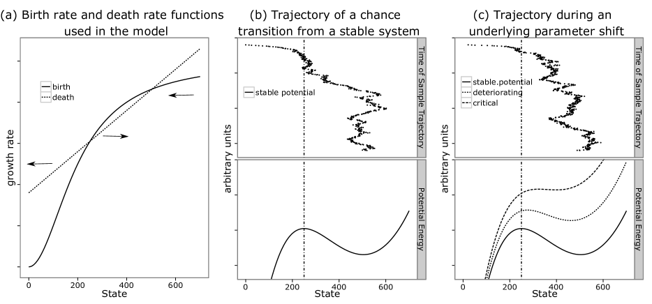
Figure 1: The Prosecutor’s Fallacy. (a) Plot of the model functions shown in Eq (2) with parameters $a=180$, $K=500$, $e=.5$, and $h=200$. When the death rate is higher than the birth rate, the system dynamics drive the state (population size) to smaller values. When birth rate is higher, the system moves right, as indicated by the arrows.(b) The potential energy is given by the negative integral of $b(n)-d(n)$, shown in the lower plot. The potential function gives an intuitive picture of the stability of a system by imagining the curve as a surface on which a ball is free to bounce across – wells correspond to stable points and peaks to unstable points. While most trajectories remain near the stable well, some transition out merely by chance. An example of such a trajectory is shown in the top panel, in which time increases along the vertical axis. Though initially oscillating around the stable state, a chance excursion carries it beyond the Allee threshold (vertical dotted line). Such chance trajectories can produce the statistical patterns as observed in true critical transitions seen in panel (c): Early warning signals are aimed at detecting systems which are slowly moving towards a tipping point or bifurcation, illustrated in the successive curves (deteriorating and critical). Top panel: An example trajectory from a simulation under this process shows the state of the system as the potential moves towards the bifurcation point. The original position of the Allee threshold is shown by the vertical dotted line (though it moves slightly as the parameter changes).

2 Methods and Results

To investigate if early warning signals are vulnerable to this fallacy, we simulate a system that is not driven towards a bifurcation such as in Fig reffig:1(b). This simulation approach allows us to determine whether examining historical events is a valid way to test the utility of these indicators. We simulated 20,000 replicates of a stochastic individual-based birth-death process with an Allee threshold (Courchamp et al., 2008), which arises from positive fitness effects at low densities. Above the Allee threshold the population returns to a positive equilibrium size, whereas below the threshold the population decreases to zero. The model can be represented as a continuous time birth-death process where births and deaths are Poisson events which depend on the current density with rates given by

$$b(n) =\frac{Kn^{2}}{n^{2}+h^{2}},$$ (2)

$$d(n) =en+a,$$ (3)

a model with a linear death rate and density-dependent birth rate that drives the Allee effect at low densities and limits growth at high densities. In this model $n$ indicates the discrete number of individuals in the population, $K$ indicates a carrying capacity as set by a limiting resource, $e$ a per-capita death rate (the $e$ scaling term in the birth equation allows the carrying capacity $K$ to correspond to a positive equilibrium point), $a$ an additional mortality imposed on the population such as harvest, $h$ is a parameter controlling at what population size the addition of more individuals switches from conferring a positive benefit on growth from Allee interactions $n<h$ to a negative impact on growth due to increased competition, $n>h$. The key feature of this model is the alternate stable states introduced by this effect; other functional forms for Eq. (2) could serve equally well for these simulations (see e.g. Scheffer et al., 2001). Though this system can be forced through a bifurcation by increasing the death rate, in these simulations all parameters are held constant and no bifurcation occurs. Consequently we do not anticipate an early warning signal of an approaching bifurcation.

The simulation starts from the positive equilibrium population size. Though the chance of a transition across the Allee threshold in any given time step is small, given enough time this system will eventually experience such a rare event driving the population extinct. We ran each replicate over 50,000 time units, sampling the system every 50 time units. In this time window 266 of the 1,000 replicates experience population collapse. To keep the examples of comparable sample size, we focus on a section of the data 500 time points prior to the system approaching the transition.

To test whether selecting systems that have experienced spontaneous transitions could bias the analysis towards false positive detection of early warning signals, (the Prosecutor’s Fallacy) we selected replicates conditional on having collapsed in the simulations. We then selected a window around each system that ended just before the collapse, while the population values were still above the Allee threshold. For each replicate, we calculated the most common early warning indicators, variance and autocorrelation (e.g. Carpenter and Brock, 2006; Dakos et al., 2008; Scheffer et al., 2009), around a moving window equal to half the length of that time series.

To test for the presence of a warning signal in these indicators we computed values of Kendall’s $\tau$ for both indicators for each of the 266 replicates. Kendall’s $\tau$ is a non-parametric measure of rank correlation frequently used to identify an increasing trend ($\tau>0)$ in early warning signals (Dakos et al., 2008, 2011), defined as $\tau{\frac{1}{2}n(n-1)}$ in $n$ observations. $\tau$ takes values in $(-1,1)$. The distribution of $\tau$ values observed across these replicates is shown in Figure 2. We compare the distribution of $\tau$ from all the simulations to the distribution conditioned on experiencing a chance transition to the alternative stable state. To avoid an effect of sample size the time series are all chosen to be the same length.

To demonstrate the effect we observe is not unique to models with Allee effects, we provide an example of the effect arising in a discrete-time model with two non-zero stable states adapted from (May, 1977),

$$X_{t+1}=X_{t}\exp\left(r\left(1-\frac{X_{t}}{K}\right)-\frac{a*X_{t}^{Q-1}}{X_{t}^{Q}+H^{Q}}\right).$$ (4)

which combines a logistic growth model with a saturating predator response (See May (1977) for detailed discussion), shown in Figure 3. Code to replicate the analysis can be found at
https://github.com/cboettig/earlywarning/tree/prosecutor/.

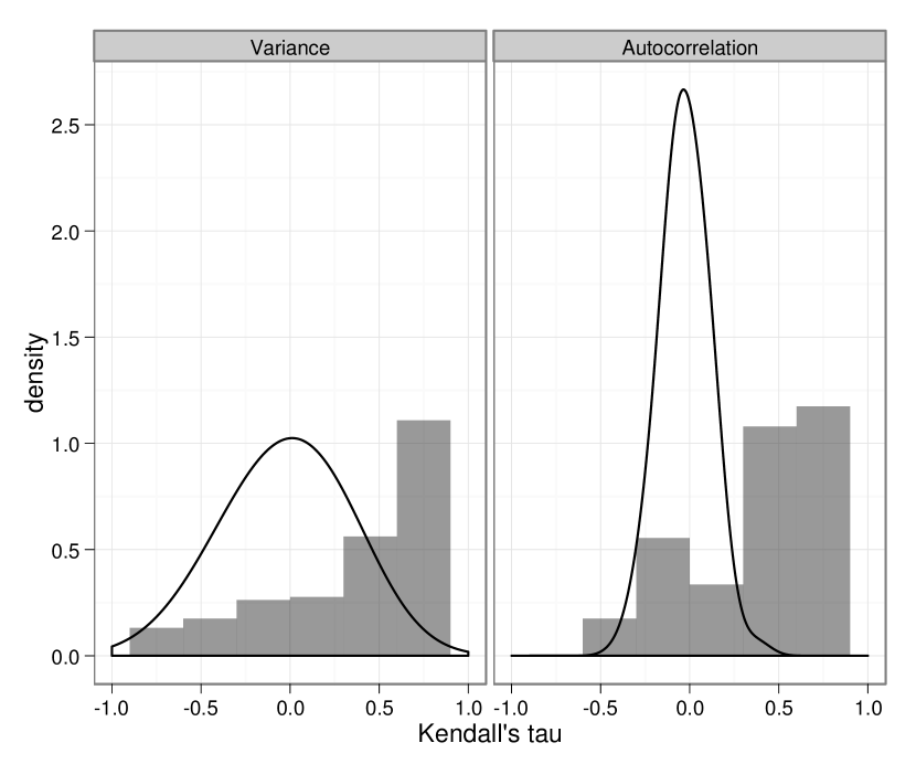
Figure 2: The distribution of the correlation statistic $\tau$ for two early warning indicators (variance, autocorrelation) on replicates conditionally selected for having collapsed by chance in simulations is shown in grey bars. Solid lines indicate the estimated density of the statistic from a random sample of the simulations (not conditional on observing a transition). Positive values of $\tau$ correspond to a pattern of an indicator increasing with time; typically taken as evidence that a system is approaching a critical transition. In these simulations, the pattern arises instead from the Prosecutor’s fallacy of conditional selection.

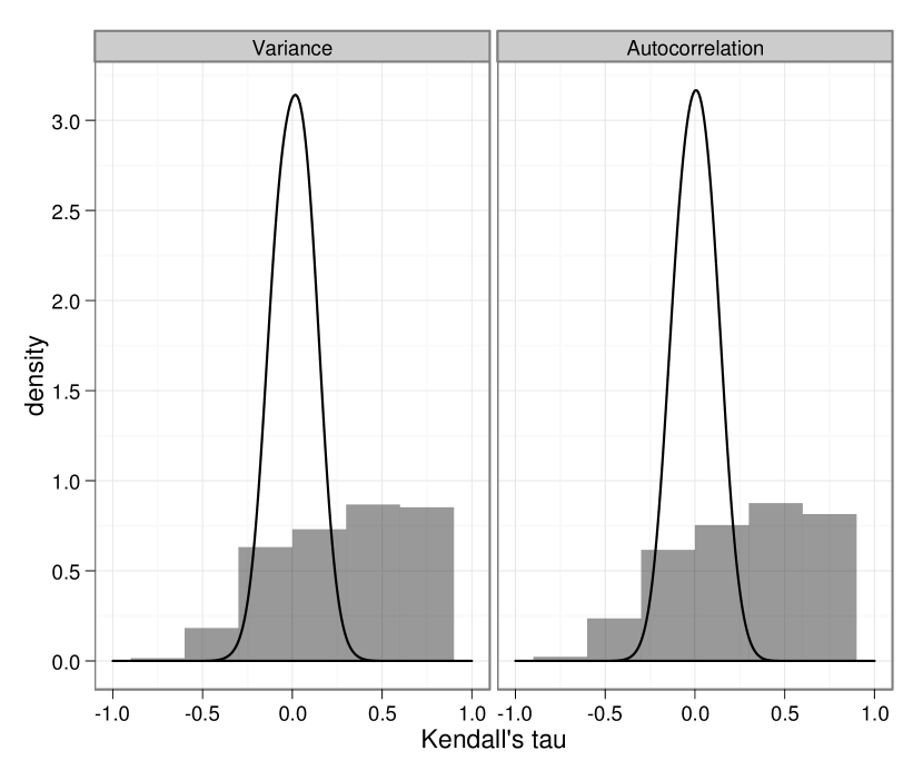
Figure 3: The identical analysis from Figure 2 is shown for the model in Eq (4) using parameters $r=0.75$, $K=10$, $a=1.7$, $Q=3$, and $H=1$. A similar statistical bias, particularly towards positive values of $tau$ occurs in this model as well.

For each of these replicates we also take a model-based approach, estimating parameters for an approximate linear model of the system approaching a saddle node bifurcation, as described by Boettiger and Hastings (2012),

$$\mathrm{d}X=\sqrt{r_{t}}(\phi(r_{t})-X_{t})\mathrm{d}t+\sigma\sqrt{\phi(r_{t})}\mathrm{d}B_{t}$$ (5)

In this model, the parameter $m$ describes the approach towards the saddle-node bifurcation. Estimates $m<0$ are expected in systems approaching a bifurcation, while for stable systems $m$ should be approximately zero. None of the estimates across the 266 simulations differed from zero in our study, hence the model-based estimation shows no evidence of bias on data that has been selected conditional on collapse.

3 Discussion

The attempts to detect early warning signs for critical transitions are based on the concept of a deteriorating environment as embodied in a changing parameter Scheffer et al. (2009), which is a different kind of transition than one which is driven instead by stochasticity in an environment which is otherwise constant and exhibiting no directional change. When trying to use historical data to understand critical transitions we often do not know which category, changing environment or simply chance, an observed large change falls into.

We have shown here that systems which undergo rare sudden transitions due to chance look statistically different from their counterparts that do not, even though they are driven by the same stochastic process. In particular, such conditionally selected examples are more likely to show signs associated with an early warning of an approaching tipping point, such as increasing variance or increasing autocorrelation, as measured by Kendall’s $\tau$. This increases the risk of false positives – cases in which a warning signal being tested appears to have successfully detected an underlying change in the system leading to a tipping point, when in fact the example comes instead from a stable system with no underlying change in parameters. Figure 2 shows that many of the chance crashes show values of $\tau$ that are significantly larger than those observed in the otherwise identical replicates that did not experience a chance transition, thus “detecting” an underlying change in the system dynamics that is not in fact present.

3.1 Chance transitions are false positives for early warning signals

It seems tempting to argue that this bias towards positive detection in historical examples is not problematic – each of these systems did indeed collapse, so the increased probability of exhibiting warning signals could be taken as a successful detection. Unfortunately this is not the case. At the moment the forecast is made, these systems are not likely to transition, since they experience a strong pull towards the original stable state. A closer look at the patterns involved shows why common indicators such as autocorrelation and variance can be misleading.

As the system gets farther from its stable point, it it more likely to draw a random step that returns it towards the stable point. Despite this, there is always some probability that it will move further still, so systems that do cross the tipping point must do so rather quickly by a string of events. This pattern, clearly visible before the crashes in each of the examples in Figure 1, produces a string of observations that appear more highly autocorrelated (if we are sampling the system frequently enough to catch the excursion at all) than we observe in the rest of the fluctuations around the equilibrium. Yet this autocorrelation comes from a chance trajectory moving quickly away from the stable state, not from the critical slowing down pattern in the return times to the stable state which precede a saddle-node bifurcation and motivate the early warning signal.

This longer than expected excursion results in a higher than expected variance in that window as well. Both variance and autocorrelation are calculated using a moving window over the time-series, which allows the method to pick out a pattern of change as the window moves along the sequence. If this chance excursion that precedes the crash happens to fill a significant part of the moving window, the resulting pattern will tend to show an increase in autocorrelation or variance. If the chance excursion is relatively rapid compared to the frequency at which the system is observed (spacing of the data) or the width of the moving window, the excursion may not significantly alter the general pattern. In this way, some of the events in which a crash is observed will appear to present these statistical patterns of increased variance or autocorrelation without being harbingers of approaching critical transitions.

3.2 The truncation of observations

If we had a complete knowledge of the system dynamics, then we could eliminate the bias we observe here since the bias arises from the transient branch of the trajectory that crosses the threshold, and if the system were truncated at the minimum of the potential then the effect we emphasize here would not appear.  But, it is not possible to truncate the system in any practical application. The precise location of the minimum of the potential which is the location of the deterministic equilibrium is unknown. Moreover, under the hypothesis that the system is approaching a critical transition, the location of the minimum potential moves so it cannot easily be estimated by previous observations, (see Figure 1c where the equilibrium point moves in the direction of the transition). Thus it is neither practical nor desirable to suggest that historical time series can be used by following a simple truncation rule that avoids the branch of a trajectory crossing the threshold to another basin of attraction.  Exactly where a particular study will choose to truncate such a trajectory will necessarily be arbitrary without an underlying model of the process.  Frequently this is done by removing the very steep, monotonic branch of the trajectory expected once the system crosses the unstable threshold.  Such an approach corresponds with our choice of termination and produces the bias we discuss here.

The examples of Figure 1, though only single replicates, may be useful in illustrating these issues.  Figure 1c, top panel shows a sample trajectory of a system with a parameter shift, while 1b shows a trajectory without a shift.  Both trajectories become more highly autocorrelated and higher variance near the end of the time series (time increases on the y axis in Figure 1).  The part of the time series following the critical transition shows a fast and monotonic trajectory to the unstable trajectory, and would usually be excluded by an analysis for warning signals in advance of the transition.  No such clear pattern exists prior to the transition in Figure 1b.   An alternative proposal to terminate the trajectory in panel B earlier would also risk decreasing the signal seen in panel c, and would be inconsistent with the application of warning signals in the forecasting context, where there would be no such truncation.

3.3 Comparing to the model-based method

In our numerical experiment, the model-based estimate of early warning signals appears more robust than the summary statistics, producing the same estimates on both the conditionally selected replicates as on a random sample of the replicates. This is a consequence of the more rigid specifications that come with a model-based approach – the pattern expected is less general than any increase in variance or autocorrelation, but instead must be one that matches its approximation of the saddle-node bifurcation. This observation highlights the difference between the pattern driving the false positive trends in increasing variance and increasing autocorrelation and the pattern anticipated in the saddle-node model. This should not however be taken as evidence that the model-based approach is immune to the bias of the Prosecutor’s Fallacy.

3.4 Importance of experimental approaches

The problem we highlight ultimately stems from the difficulty of having only a single realization with which to examine a complex problem. The only way to deal with this problem embodied is through replication, as can be done in an experimental system in laboratory manipulations such as Drake and Griffen (2010); Veraart et al. (2011); Dai et al. (2012) and at the scale of whole lake ecosystems in Carpenter (2011). Experimental procedures avoid the hazard of the Prosecutor’s fallacy by generating a complete sample of replicates, rather than selecting a subset of cases from some larger historical sample.

4 Acknowledgments

This research was supported by funding from NSF Grant EF 0742674 to AH and a Computational Sciences Graduate Fellowship from the Department of Energy grant DE-FG02-97ER25308 and NERSC Supercomputing grant DE-AC02-05CH11231 to CB. The authors thank M. Baskett, T.A. Perkins and N. Ross for helpful comments on earlier drafts of the manuscript, and also P. Ditlevsen and an anonymous reviewer for their comments.

References

- Berkes et al. (2006) Berkes, F., Hughes, T. P., Steneck, R. S., Wilson, J. A., Bellwood, D. R., Crona, B., Folke, C., Gunderson, L. H., Leslie, H. M., Norberg, J., Nyström, M., Olsson, P., Osterblom, H., Scheffer, M., Worm, B., Mar. 2006. Ecology. Globalization, roving bandits, and marine resources. Science (New York, N.Y.) 311 (5767), 1557–8.
- Boettiger and Hastings (2012) Boettiger, C., Hastings, A., May 2012. Quantifying limits to detection of early warning for critical transitions. Journal of The Royal Society Interface 9 (75), 2527 – 2539.
- Carpenter (2011) Carpenter, J., Feb. 2011. May the Best Analyst Win. Science 331 (6018), 698–699.
- Carpenter and Brock (2006) Carpenter, S. R., Brock, W. A., 2006. Rising variance: a leading indicator of ecological transition. Ecology letters 9 (3), 311–8.
- Courchamp et al. (2008) Courchamp, F., Berec, L., Gascoigne, J., 2008. Allee Effects in Ecology and Conservation. Oxford University Press, USA.
- Dai et al. (2012) Dai, L., Vorselen, D., Korolev, K. S., Gore, J., May 2012. Generic Indicators for Loss of Resilience Before a Tipping Point Leading to Population Collapse. Science 336 (6085), 1175–1177.
- Dakos et al. (2011) Dakos, V., Kéfi, S., Rietkerk, M., Nes, E. H. V., Scheffer, M., 2011. Slowing Down in Spatially Patterned Ecosystems at the Brink of Collapse. The American Naturalist.
- Dakos et al. (2008) Dakos, V., Scheffer, M., van Nes, E. H., Brovkin, V., Petoukhov, V., Held, H., Sep. 2008. Slowing down as an early warning signal for abrupt climate change. Proceedings of the National Academy of Sciences 105 (38), 14308–12.
- Ditlevsen and Johnsen (2010) Ditlevsen, P. D., Johnsen, S. J., Oct. 2010. Tipping points: Early warning and wishful thinking. Geophysical Research Letters 37 (19), 2–5.
- Drake and Griffen (2010) Drake, J. M., Griffen, B. D., Sep. 2010. Early warning signals of extinction in deteriorating environments. Nature 467 (7314), 456–459.
- Guttal and Jayaprakash (2008) Guttal, V., Jayaprakash, C., Dec. 2008. Spatial variance and spatial skewness: leading indicators of regime shifts in spatial ecological systems. Theoretical Ecology 2 (1), 3–12.
- Hirota et al. (2011) Hirota, M., Holmgren, M., Van Nes, E. H., Scheffer, M., Oct. 2011. Global Resilience of Tropical Forest and Savanna to Critical Transitions. Science 334 (6053), 232–235.
- Kéfi et al. (2007) Kéfi, S., Rietkerk, M., Alados, C. L., Pueyo, Y., Papanastasis, V. P., Elaich, A., de Ruiter, P. C., Sep. 2007. Spatial vegetation patterns and imminent desertification in Mediterranean arid ecosystems. Nature 449 (7159), 213–7.
- Lenton (2011) Lenton, T. M., Jun. 2011. Early warning of climate tipping points. Nature Climate Change 1 (4), 201–209.
- Lenton et al. (2012) Lenton, T. M., Livina, V., Dakos, V., 2012. Early warning of climate tipping points from critical slowing down: comparing methods to improve robustness. Philosophical Transactions of The Royal Society A (in press).
- Livina and Lenton (2007) Livina, V. N., Lenton, T. M., Feb. 2007. A modified method for detecting incipient bifurcations in a dynamical system. Geophysical Research Letters 34 (3), 1–5.
- May (1977) May, R. M., Oct. 1977. Thresholds and breakpoints in ecosystems with a multiplicity of stable states. Nature 269 (5628), 471–477.
- Mumby et al. (2007) Mumby, P. J., Hastings, A., Edwards, H. J., Nov. 2007. Thresholds and the resilience of Caribbean coral reefs. Nature 450 (7166), 98–101.
- Scheffer et al. (2009) Scheffer, M., Bascompte, J., Brock, W. A., Brovkin, V., Carpenter, S. R., Dakos, V., Held, H., van Nes, E. H., Rietkerk, M., Sugihara, G., 2009. Early-warning signals for critical transitions. Nature 461 (7260), 53–9.
- Scheffer et al. (2001) Scheffer, M., Carpenter, S. R., Foley, J. A., Folke, C., Walker, B., Oct. 2001. Catastrophic shifts in ecosystems. Nature 413 (6856), 591–6.
- Supreme Court (1968) Supreme Court, C., 1968. People v. Collins.
- Thompson and Sieber (2010) Thompson, J. M. T., Sieber, J., Dec. 2010. Climate tipping as a noisy bifurcation: a predictive technique. IMA Journal of Applied Mathematics 76 (1), 27–46.
- Thompson and Schumann (1987) Thompson, W. C., Schumann, E. L., 1987. Interpretation of statistical evidence in criminal trials: The prosecutor’s fallacy and the defense attorney’s fallacy. Law and Human Behavior 11 (3), 167–187.
- van Nes and Scheffer (2007) van Nes, E. H., Scheffer, M., Jun. 2007. Slow recovery from perturbations as a generic indicator of a nearby catastrophic shift. The American naturalist 169 (6), 738–47.
- Veraart et al. (2011) Veraart, A. J., Faassen, E. J., Dakos, V., van Nes, E. H., Lürling, M., Scheffer, M., Dec. 2011. Recovery rates reflect distance to a tipping point in a living system. Nature, 2–5.