High Energy Neutrinos from Dissipative Photospheric Models of
Gamma Ray Bursts

Abstract

We calculate the high energy neutrino spectrum from gamma-ray bursts where the emission arises in a dissipative jet photosphere determined by either baryonically or magnetically dominated dynamics, and compare these neutrino spectra to those obtained in conventional internal shock models. We also calculate the diffuse neutrino spectra based on these models, which appear compatible with the current IceCube 40+59 constraints. While a re-analysis based on the models discussed here and the data from the full array would be needed, it appears that only those models with the most extreme parameters are close to being constrained at present. A multi-year operation of the full IceCube and perhaps a next generation of large volume neutrino detectors may be required in order to distinguish between the various models discussed.

I Introduction

Gamma-ray bursts (GRBs) are a potential source of astrophysical high energy neutrinos which are currently being investigated with IceCube. The standard GRB internal shock scenario of neutrino production Waxman and Bahcall (1997); Guetta et al. (2004) used so far to compare against the IceCube 40 string and 40+59 string observations Abbasi et al. (2011, 2012) assumed some simplifications in the neutrino physics. Also, the astrophysical model itself of the GRB prompt gamma-ray emission based on the same internal shocks has been the subject of discussions in the gamma-ray community Ghisellini and Celotti (1999); Preece et al. (2000); Medvedev et al. (2004); Meszaros (2006), due to issues with the radiation efficiency and the spectral properties in the standard version of this internal shock scenario.

For this reason, modified internal shock models that address these issues (e.g. (Asano and Terasawa, 2009; Inoue et al., 2011; Murase et al., 2012; Zhang and Yan, 2011)) as well as alternative models where the prompt gamma-ray emission arises in the jet photosphere have been considered (e.g. (Mészáros and Rees, 2000; Ryde, 2005; Rees and Mészáros, 2005; Pe’er et al., 2006; Beloborodov, 2010; Pe’er, 2011). In such photospheric models the high radiative efficiency is due to dissipation processes in it.

A separate question that has also been the subject of debate in the astrophysics community is whether the jets in such relativistic sources are dominated by the baryons or by magnetic fields, which imply different macroscopic acceleration rates, different proper densities in the jet rest-frame, and implying a major role for magnetic dissipation in the process of particle acceleration. Such magnetically dominated jets in GRBs have been investigated by Drenkhahn (2002); Tchekhovskoy et al. (2010); Metzger et al. (2011); McKinney and Uzdensky (2012) and others, and the gamma-ray emission is ascribed in such models, again, to dissipative processes mainly in the photosphere, e.g. Giannios and Spruit (2007); Veres and Mészáros (2012).

It is unclear at present whether the above mentioned modified internal shocks or the photospheric models are best for interpreting the prompt gamma-ray emission, nor whether the jet dynamics is dominated by baryonic or magnetic stresses (e.g. Mészáros and Gehrels (2012)). However, the expected neutrino emission is strongly dependent on the specific overarching dissipation and dynamic model of GRBs. For this reason, here we explore the neutrino features of the three main types of models which are currently under consideration. We illustrate the variety of astrophysical uncertainties involved in these models, and how these can affect the expectations for detection with IceCube or future instruments.

II The Dissipative Photospheric Scenarios

In the typical GRB model a high energy-to-mass ratio, jet-like relativistic outflow is launched which initially accelerates with a bulk Lorentz factor $\Gamma$, averaged over the jet cross section, whose dependence on distance from the center of the explosion can be parametrized as

$$\Gamma=(r/r_{0})^{\mu}.$$ (1)

This behavior is assumed valid up to a saturation radius $r_{\rm sat}=r_{0}\eta^{1/\mu}$, where the Lorentz factor has reached the asymptotic value $\Gamma_{\rm sat}=\eta$, where $\eta\simeq L/{\dot{M}}c^{2}$ is the dimensionless entropy of the outflow, $L$ and ${\dot{M}}$ being the average energy and mass flux. The index $1/3\lesssim\mu\lesssim 1$ ranges between the extreme $\mu=1/3$ magnetically dominated radial outflow and the usual $\mu=1$ baryonically dominated outflow regimes, e.g. (Mészáros and Rees, 2011a). In the extreme magnetic case and baryonic cases, the saturation radius is given by

$$r_{\rm sat}=\begin{cases}\eta^{3}r_{0}\sim 2.7\times 10^{14}\eta_{300}r_{0,7}~{}{\rm cm},&~{}~{}{\rm for}~{}~{}\mu=1/3\\ \eta r_{0}\sim 3\times 10^{9}\eta_{300}r_{0,7}~{}{\rm cm},&~{}~{}{\rm for}~{}~{}\mu=1.\end{cases}$$ (2)

In the dissipative photospheric scenario, a fraction of the outflow bulk kinetic energy is converted into radiation energy via some dissipation mechanism in the neighborhood of the photosphere., giving rise to the “prompt" photon luminosity $L_{\gamma}=\epsilon_{e}L_{\rm tot}$, where $L_{\rm tot}=10^{53}L_{53}$ erg/s is the isotropic equivalent total luminosity of the jet. The photospheric radius is estimated by setting the Thomson optical depth $\tau_{{\gamma}e}\sim{n^{\prime}_{e}}\sigma_{T}R_{\rm ph}/\Gamma=1$, where $n^{\prime}_{e}=n^{\prime}_{p}\approx L_{\rm tot}/4\pi R_{\rm ph}^{2}m_{p}c^{3}\eta\Gamma$ is the comoving density of electrons if the $e^{+}e^{-}$ pairs are absent. By using Eqn.1 and the condition above, we obtain

$$\frac{R_{\rm ph}}{r_{0}} = \left(\frac{L_{\rm tot}\sigma_{T}}{{4\pi}m_{p}c^{3}r_{0}}\right)\frac{1}{\eta\Gamma_{ph}^{2}}=$$ (5)

$$= \left\{\begin{array}[]{ll}\eta_{T}^{1/\mu}(\eta_{T}/\eta)^{3}&{\rm if~{}}\eta<\eta_{T}\\ \eta_{T}^{1/\mu}(\eta_{T}/\eta)^{1/(1+2\mu)}&{\rm if~{}}\eta>\eta_{T}\end{array}\right.$$

(Veres and Mészáros, 2012), where

$$\eta_{T}=\left(\frac{L_{\rm tot}\sigma_{T}}{4\pi m_{p}c^{3}r_{0}}\right)^{\frac{\mu}{1+3\mu}}.$$ (6)

Typically, for a magnetically dominated $\mu=1/3$ case the photosphere occurs in the acceleration phase $r\leq r_{\rm sat}$, if $\eta>\eta_{T}$, where $\eta_{T}\simeq 150L_{53}^{1/6}r_{0,7}^{-1/6}$. On the other hand the photosphere occurs in the coasting phase $r>r_{\rm sat}$ for $\eta<\eta_{T}$, which is typical for baryonic cases, where $\mu=1$ and $\eta_{T}\simeq 1900~{}L_{53}^{1/4}r_{0,7}^{-1/4}$. The Lorentz factor of the photosphere $\Gamma_{\rm ph}$ has an $r_{\rm ph}$ dependence for $\eta>\eta_{T}$, being $\Gamma_{\rm ph}=(r_{\rm ph}/r_{0})\propto L^{\mu/(2\mu+1)}\eta^{-\mu/(2\mu+1)}r_{0}^{-\mu/(2\mu+1)}$, while $\Gamma_{\rm ph}\approx\eta$ in the case $\eta<\eta_{T}$.

In the baryonic photospheres the dissipation may be due to dissipation of MHD turbulence (Thompson, 1994) or it may occur in the form of semi-relativistic shocks Rees and Mészáros (2005) with Lorentz factor $\Gamma_{r}\sim 1$, of different kinematic origin but similar physical properties as internal shocks, with a mechanical dissipation efficiency $\epsilon_{d}$. These result in a proton internal energy, and result also in random magnetic fields with an efficiency $\epsilon_{B}$, relativistic protons with $\epsilon_{p}$, and relativistic electrons with $\epsilon_{e}$. In the magnetically dominated jets the total jet luminosity $L_{\rm tot}$ in the acceleration phase before dissipation occurs consists of a toroidal magnetic field component and a proton bulk kinetic energy component. In the dissipation region a fraction $\epsilon_{d}$ of $L_{\rm tot}$ is assumed to be dissipated, consuming a fraction from each of the toroidal field and bulk proton energy, and resulting in proton internal energy and in a fraction $\epsilon_{B}$ which appears as random magnetic fields, and $\epsilon_{p}$ and $\epsilon_{e}$ which appear as relativistic protons and relativistic electrons. In both baryonic and magnetically dominated cases we assume $\epsilon_{B}+\epsilon_{p}+\epsilon_{e}=1$, and we take $\epsilon_{d}\sim 0.3$ and $\epsilon_{B}\sim 1/3$ as examples in this paper. In the jet comoving frame the random magnetic field after the dissipation is parametrized by an energy density

$$U_{\rm B,random}^{\prime}=B^{\prime 2}/{8\pi}=\kappa\epsilon_{B}\epsilon_{d}L_{\rm tot}/(4\pi{R_{\rm ph}^{2}}\Gamma_{\rm ph}^{2}c)$$ (7)

where for semi-relativistic shocks ($\Gamma_{\rm rel}\sim 1$), and a compression ratio of $\kappa\sim 4$ is assumed. For the magnetically dominated outflow, during the acceleration phase, the energy remaining in toroidal fields after dissipation is

$$U_{\rm B,toroid}^{\prime}=(1-\epsilon_{d})(1-\Gamma_{\rm ph}/\eta)L_{\rm tot}/(4\pi{R_{\rm ph}^{2}}\Gamma_{\rm ph}^{2}c)$$ (8)

where $\Gamma_{\rm ph}$ is the bulk Lorentz factor of the protons at the photosphere.

Calculations and simulations of of such baryonic and magnetic dissipative photospheres as well as internal shocks generally result in an escaping photon spectrum similar to the observed characteristic “Band" spectrum (Band et al., 1993), parametrized as

$$dN_{\gamma}/dE\propto(E/E_{\rm br})^{x_{\rm ph}}$$ (9)

in the observer frame. Observationally, for average bursts at redshifts $z\sim 2$ the mean values are $E_{\rm br}\sim 300$ keV, $x_{\rm ph}=-1$ below $E_{\rm br}$ and $x_{\rm ph}=-2$ above $E_{\rm br}$. In a photosphere this spectral shape is the product of the modification of a thermal spectrum by the dissipation. For the purposes of this article, we treat this photon spectrum as the input for our calculations, transformed to the rest frame of the outflow. While the bulk Lorentz factors in the photosphere and internal shock models may differ, for the purposes of comparison we adopt here as a test case the same comoving frame photon spectral break energy for the dissipation zones of the various models considered, $E_{\rm br}^{\prime}=0.01$ MeV, and $x_{\rm ph}=-1$ below $E_{\rm br}^{\prime}$ and $x_{\rm ph}=-2$ above $E_{\rm br}^{\prime}$. The lower and upper branches can have cut-off energies, e.g. determined by synchrotron self-absorption below and acceleration restrictions or $\gamma\gamma\to{e^{+}e^{-}}$ pair production above, the cut-off values depending on the specific model and its parameters. For simplicity, here we adopt the same constant values of a lower limit $E_{\rm min}^{\prime}=1$ eV and an upper limit $E_{\rm max}^{\prime}=0.5$ MeV, which are adequate for our purposes since the neutrino results are insensitive to these values. The total luminosity of this Band-function spectrum is normalized to $\epsilon_{d}\epsilon_{e}L_{\rm tot}$, where $L_{\rm tot}$ represents the total luminosity. (An additional softer thermal spectral component can also be present at the photosphere. However, the temperature of this component is estimated as $T\sim{o(1)\times{\rm keV}}$ at the photosphere (Veres and Mészáros, 2012), corresponding to a thermal luminosity $L_{\rm thermal}\sim{o(1)}\times 10^{49}{\rm erg/s}$ which is low compared to $L_{\rm tot}$ and $L_{\gamma}$. Hence we have neglected this component for the purposes of the present neutrino calculation.)

When the outflow encounters the external medium, it starts to decelerate at a radius

$$R_{d} \approx(\frac{3L_{\rm tot}t_{\rm dur}}{4{\pi}n_{\rm ISM}m_{p}c^{2}\eta^{2}})^{1/3}$$

$$=2.54\times 10^{16}L_{t,53}^{1/3}(t_{\rm dur}/10s)^{1/3}n_{\rm ISM,2}^{-1/3}\eta_{300}^{-2/3}$$ (10)

where an external shock forms which is also able to produce neutrinos. Here we have assumed a uniform interstellar medium of particle density $n_{\rm ISM}=10^{2}n_{\rm ISM,2}cm^{-3}$ and a jet outflow duration time $t_{\rm dur}$ in the central engine frame. The interstellar density value does not affect the photospheric or internal shock neutrinos, but it does affect the external shock neutrinos. Here we have adopted a density which is optimistic for the external shock neutrinos, since even so the external neutrino fluxes predicted are low and more moderate densities such as the typically used $n_{\rm ISM}=1\rm cm^{-3}$ would lead to even smaller external shock neutrino fluxes. The corresponding deceleration timescale is estimated as $t_{d}^{\prime}\sim{R_{d}}/c\eta$. At this radius deceleration $R_{d}$ the external shock has fully developed, consisting of a forward shock, and possibly also a reverse shock (if the magnetization parameter $\sigma$ is or has become low enough at this radius). If present, for our parameters the reverse shock is marginally in the so-called thin-shell regime, the reverse shock having become semi-relativistic as it crosses the ejecta at about the deceleration time $t_{d}$.

The turbulent magnetic fields generated in these external shocks lead to synchrotron radiation, as well as synchrotron self-Compton (SSC) and external inverse Compton (EIC) scattering of non-thermal photons from the dissipation region near the photosphere or the internal shocks. The detailed method of calculation of these photon spectra are discussed in (Veres and Mészáros, 2012; Toma et al., 2011; Asano et al., 2011). As shown below, however, the neutrino fluence from the external shock region is a few orders of magnitude lower than that from the photospheric or baryonic internal shock regions, due to a much lower photon density leading to a lower interaction rate and lower pion production efficiency. Under the assumptions made here, the input photon spectrum of a GRB with typical parameters is shown in Fig.1 as an example. For the reverse shock, we include both the self-generated photons from the reverse shock and the prompt emission as target photons for inverse Compton scattering as well as for $p\gamma$ interaction. For the forward shock, we include the forward shock (FS), reverse shock (RS) and prompt photons.

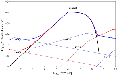
Figure 1: Photon spectrum in the observer frame for a typical GRB with parameters $L_{\rm tot}=5\times 10^{52}$ erg/s, $t_{\rm dur}=10$ s, $\eta=300$ , $z=1.0$, $n_{\rm ISM}=100~{}\rm cm^{-3}$ , $\epsilon_{\rm d}=0.3$, $\epsilon_{\rm e}=\epsilon_{\rm p}=\epsilon_{\rm B}=1/3$, where $\epsilon_{\rm d}$ is defined as the total dissipated energy from jet total energy, in the forms of $\epsilon_{\rm e}$,$\epsilon_{\rm p}$ and $\epsilon_{\rm B}$. The subindex "ph" refers to photosphere, “prompt" refers to the prompt emission from the photospheric region, for which a Band-like spectrum is assumed. The SYN,R and SYN,F are the synchrotron from the reverse and forward shock; SSC is the synchrotron-self Compton spectrum, EIC is the inverse Compton scattering of the prompt photons in the external shock region. (At very high energies, a Klein-Nishina break may be expected; however, for the neutrino calculation this contribution can be neglected since it contains very few photons, hence these KN breaks are not shown here). A smaller dissipation value for external shock emission used , $\epsilon_{\rm B,FS}=\epsilon_{\rm B,RS}=0.02\epsilon_{\rm B}$, suitable to explain the external shock photon emission (Veres and Mészáros, 2012).

III method of calculation

In the baryonic dissipation regions, whether these are in the photosphere or in internal shocks beyond the photosphere, it is usually assumed that protons, as well as electrons, are accelerated through a Fermi-first order (Fermi-I) acceleration mechanism in the disordered magnetic fields created in the region. A process similar to Fermi acceleration is also expected in magnetic reconnection regions where layers of magnetic field of opposite polarity meet and drive converging flows. (Kowal et al., 2009; Sironi and Spitkovsky, 2011; Hoshino, 2012). The particles bounce back and forth in the converging flow between the layers and can reach similar maximum energies as in the usual Fermi mechanism. We assume that the injection of accelerated protons has a spectrum

$$dN_{p}/dE\propto{E}^{-x_{p}}\hskip 14.22636pt(E_{\rm p,min}<E_{\rm p}<E_{\rm p,max})$$ (11)

with $x_{p}=2$ as a nominal value. The acceleration timescale is $t_{\rm acc}^{\prime}\sim{t_{\rm cycle}^{\prime}}=\xi_{p}r_{g}^{\prime}/c=\xi_{p}E_{p}^{\prime}/eB^{\prime}c$ , where $r_{g}$ is the average gyroradius. Here we have adopted a minimum injection energy of protons $E_{\rm p,min}^{\prime}=10$ GeV since the neutrino spectrum is insensitive to this value. We have also assumed a high compression ratio and weakly disordered magnetic fields, corresponding to $\xi_{p}\sim 10$. The accelerated proton spectral energy (eqn.11) here is normalized to a fraction of the jet total luminosity $\epsilon_{p}L_{\rm tot}$, the value of $\epsilon_{p}$ being discussed in section IV.

The maximum proton energy is constrained by the gyroradius being smaller than the size of the acceleration region $r_{g}^{\prime}<R_{\rm ph}/\Gamma_{\rm ph}$, or by radiative cooling $t_{\rm p,acc}<t_{\rm p,cool}$ where $t_{\rm p,cool}$ is the total cooling timescale for the proton $t_{\rm p,cool}^{-1}=t_{\rm p\gamma}^{-1}+t_{pp}^{-1}+t_{BH}^{-1}+t_{sy}^{-1}+t_{IC}^{-1}+t_{ad}^{-1}$. The terms on the right hand side are the photohadronic, $pp$ collisional, Bethe-Heitler (photopair), proton synchrotron, inverse Compton and adiabatic inverse cooling timescales in the fluid comoving frame (we have dropped the "prime" superscript here), given respectively by

$$t_{p\gamma}^{-1} {\approx}\frac{c}{2\gamma_{p}^{2}}\int_{0}^{\infty}\frac{dE}{E^{2}}n_{ph}(E)\int_{\epsilon_{\rm TH}}^{2\gamma_{p}E}d{\epsilon}\epsilon{\sigma_{p\gamma}}(\epsilon)K_{p\gamma}(\epsilon)$$ (12)

$$t_{pp}^{-1} =cn_{p}\sigma_{pp}(\gamma_{p})K_{pp}(\gamma_{p})$$ (13)

$$t_{BH}^{-1} \approx\frac{7(m_{e}c^{2})^{2}\alpha_{f}\sigma_{T}c}{9\sqrt{2}{\pi}m_{p}c^{2}\gamma_{p}^{2}}\int_{{\gamma_{p}}^{-1}}^{\infty}d\gamma_{e}\gamma_{e}^{-2}n_{ph}(\gamma_{e}m_{e}c^{2})$$

$$\times\{(2\gamma_{p}\gamma_{e})^{3/2}[\log(2\gamma_{p}\gamma_{e})-2/3]+2/3\}$$ (14)

$$t_{sy}^{-1} =4\sigma_{T}m_{e}^{2}\gamma_{p}(B^{2}/8\pi)/3m_{p}^{3}c$$ (15)

$$t_{IC}^{-1} =\frac{3(m_{e}c^{2})^{2}\sigma_{T}c}{16\gamma_{p}^{2}(\gamma_{p}-1)\beta_{p}}\int_{0}^{\infty}\frac{dE}{E^{2}}F(E,\gamma_{p})n_{ph}(E)$$ (16)

$$t_{ad}^{-1} \approx{\Gamma{c}/R}$$ (17)

where each individual cooling inverse timescale is defined as $t^{-1}\equiv-(d\gamma_{p}/dt)\gamma_{p}$ and $n_{ph}(E)\equiv{dN/dEdV}$ is the photon differential spectral density. Neutrinos result mainly from charged pion and kaon decays, to the first and second leading order of approximation respectively here. These charged mesons come from $p\gamma$ and $pp$ interactions (eqn.12,13). The cross section and inelasticity in the former channel, considering the lower threshold $\epsilon_{\rm TH}=0.2$ GeV, are approximated by two step-functions:

$$\sigma_{p\gamma}(\epsilon) =\begin{cases}340{~{}\mu}b&0.2<\epsilon/GeV<1.0\\ 120{~{}\mu}b&\epsilon>1.0\end{cases}$$ (18)

$$K_{p\gamma}(\epsilon) =\begin{cases}0.2&0.2<\epsilon<1.0\\ 0.6&\epsilon>1.0\end{cases}$$ (19)

where $\epsilon$ is the photon energy in the proton comoving frame. For $0.2<\epsilon<1.0$ GeV the cross section is dominated by resonances while for $\epsilon>1.0$ GeV multi-pion production takes over. In the single-pion resonance channel, $\pi^{+}$ and $\pi^{0}$ are created at approximately the same rate. In the multi-pion channel, we assume that pions are created with an average multiplicity of 3, and in a first-order approximation the $\pi^{+}$ , $\pi^{-}$ and $\pi^{0}$ come in equal numbers. (For more details, see e.g. (Dermer and Menon, 2009)). For $pp$ interactions, the (thermal) protons which are not accelerated in the fluid are the targets. In the fluid comoving frame, where the target protons are basically at rest, the incident proton with energy $E_{p}(E_{p}\gg 1$ GeV) has a cross section approximated by

$$\sigma_{\rm pp}{\approx}\sigma_{\rm pp,inel}\approx 30[0.95+0.06\log(E_{p})]{\rm~{}mb}$$ (20)

with charged pion multiplicity approximated by

$$\chi(s){\approx}1.17+0.3\log{s}+0.13\log^{2}s$$ (21)

in which $s$ is the invariant energy $\sqrt{s}$ squared of the binary particle system. The detailed pion spectra are discussed in e.g. (Kamae et al., 2006; Gao and Mészáros, 2012). However, in this paper we take the approximation that the pions are created at rest in the CM frame of the binary particle system. The error caused by this approximation is much reduced in the calculation of a broad spectrum in the high energy regimes (compared with the case in (Kamae et al., 2006) or (Gao and Mészáros, 2012)),and is smaller than the astrophysical uncertainties in this paper.

To derive eqn.14, we have used a cross section $\sigma_{\phi{e}}\approx(7/6\pi)\alpha_{f}\sigma_{T}\log(\epsilon_{\gamma}/2m_{e}c^{2})$ where $\alpha_{f}=1/137$ is the fine structure constant, $\sigma_{T}=665\rm mb$ is the Thomson cross section and $\epsilon$ is the photon energy in the proton rest frame. We note that although $p\gamma{\to}p{e^{\pm}}$ has a larger cross section than the photopion process, the effective inelasticity of the proton is smaller and the relative photopion and photopair energy loss rate for protons interacting with the peak of the $\nu{F}_{\nu}$ target photon spectrum is $K_{\phi\pi}\sigma_{\phi\pi}/K_{\phi{e}}\sigma_{\phi{e}}\approx 100$. An expression for the function $F(E,\gamma_{p})$ in eqn.16 is given by (Jones, 1965). With the above analytical approximate expressions we can calculate the energy fraction from the parent proton spectrum converted into pions, $f_{p\gamma}{\equiv}t_{\rm p\gamma}^{-1}/t_{\rm p,cool}^{-1}$ and $f_{pp}{\equiv}t_{pp}^{-1}/t_{\rm p,cool}^{-1}$. With the leading order approximation that the pions are created at the rest frame of the protons, we can obtain the pion spectrum. We also rouphly approximate the produced Kaon number density as $1\sim 10$% of the pions from $p\gamma$ or $pp$ interactions, motivated by (Asano and Nagataki, 2006; Ando and Beacom, 2005) or simulations using PYTHIA-8. Neutrinos from Kaon decays are generally subdominant but they become the main component at the high end of the neutrino spectrum. At these energies charged Kaons suffer less from radiative cooling than charged Pions due to their larger mass and shorter lifetime. The various cooling timescales for a GRB with typical parameters are shown in Fig.2.

Figure 2: Proton inverse cooling timescales at the photosphere as a function of proton energy in the magnetic reconnection region comoving frame, defined as $t^{-1}=|Edt/dE|$ in s^-1. The symbols used are Triangle(pg): $p$-gamma (photopion) interaction; Circle(bh): Bethe-Heitler (photopair); Square(pp): $pp$ interaction; Dot(sy): proton synchrotron; Cross (ic) : proton inverse Compton; Solid line(ad): adiabatic cooling; Plus(ac) : Fermi acceleration timescale; Minus(TOTAL) : total cooling timescale. The astrophysical parameters for this GRB are $L_{\rm tot}=10^{53.5}$ erg/s, $\eta=300$. At lower energies, protons are mainly cooled by adiabatic expansion and $pp$ collisions. At intermediate energies in this figure, protons are mainly cooled by photopion production and at higher energies by proton synchrotron radiation.

The pion decay kinematics are well established. Neutrinos result mainly from the following channel:

$$\pi^{\pm}\rightarrow\mu^{\pm}+\nu_{\mu}(\bar{\nu}_{\mu})\rightarrow e^{\pm}+\nu_{e}(\bar{\nu}_{e})+\nu_{\mu}+\bar{\nu}_{\mu}~{}.$$ (22)

which we calculate in detail following the method in (Marscher et al., 1980). A high energy pion may lose a significant fraction of its energy through synchrotron radiation before it decays. Therefore we first calculate the pion spectrum after the cooling process has set in (using a method similar to eqns.[15,16 and 17]). Then we calculate the neutrino spectrum from the ’final’ pion and muon spectra. The $\mu^{\pm}$ has a longer mean life-time and smaller mass which makes its synchrotron cooling more severe than that of charged pions. Finally we note that the leading decay channel of the charged kaon is the same as that of the charged pion so in this sense they can be viewed as "effective pions".

While the maximum proton energy at injection is determined by the condition $t_{\rm acc}<t_{\rm cool}$, the maximum cosmic ray energy of the escaped protons can be smaller, being given by the condition $t_{\rm cool}>t_{\rm dyn}$. The resultant values are summarized in Table.1.

IV Parameters and Neutrinos from a Single Source

We numerically compute the neutrino spectrum by using the method described in the previous section. Several parameters are needed: the jet total luminosity $L_{\rm tot}$ and its duration in the source frame $t_{\rm dur}$, the target photon luminosity $L_{\gamma}=\epsilon_{d}\epsilon_{e}L_{\rm tot}$, the Fermi accelerated proton luminosity and its power-law spectral index $x_{p}$, the magnetic field calculated from the parameter $\epsilon_{B}$ and eqn.7, the dissipation radius $R$, the outflow energy to mass ratio $\eta$ and finally the source redshift $z$.

Table 1: Parameter list for different models calculated. The common parameters are: jet total luminosity $L_{\rm tot}=10^{53.5}$ erg/s, source frame duration $t_{\rm dur}=10$ s. source redshift $z=0.1$, and the dissipation partition fractions $\epsilon_{\rm e}=\epsilon_{\rm B}=\epsilon_{\rm p}=1/3$ with $\epsilon_{\rm d}=0.3$ . The first column identifies the different curve symbols and the figure used. The M and B in the second column refer to "Magnetic dominated" and "Baryonic dominated". The third column identifies the type of dissipation region: Ph for photosphere with $R_{\rm ph}$ from eqn.5, $e^{\pm}{\rm Ph}$ for pair-photosphere, and IS for internal shock of radius $R_{\rm IS}$ from eqn. 24. In the next columns $R\equiv 10^{13}R_{13}$ cm gives the corresponding radii, $\eta_{100}$ is the initial dimensionless entropy, $\Gamma_{100}@R$ and $B_{5}=B_{5}@R$ are the bulk Lorentz factor and comoving magnetic field (in the unit of $10^{5}$ G) in the dissipation region. The max $E_{\rm CR,PeV}$ is the maximum escaping cosmic ray (proton) energy in the source frame, calculated by setting $t_{\rm p\gamma}=t_{\rm dyn}$, or $t_{\rm p,syn}=t_{\rm dyn}$, or $t_{\rm p,cool}=t_{\rm p,acc}$, whichever gives the smallest $E$. The number of $\mu$-events are in the last two columns; these are estimated from the neutrino flux and the effective area of the IceCube 86-string configuration, for a source at $z=0.1$ or $z=1.0$.

We discuss three main representative scenarios: an extreme magnetic photosphere model where $\Gamma\propto{r}^{1/3}$, a baryonic photosphere model where $\Gamma\propto{r}$, and a modified internal shock (IS) scenario where two ejecta shells of different bulk Lorentz factors collide. For the modified internal shocks we assume that a high mechanical dissipation efficiency $\epsilon_{d}$ is achieved, e.g. (Asano and Terasawa, 2009; Inoue et al., 2011; Murase et al., 2012), and that the photon spectral issues raised about traditional internal shocks are avoided in such mechanisms. As far as neutrino production, the location and seed photon spectrum is similar to that in the standard internal shock, but without the simplifications of Guetta et al. (2004); Abbasi et al. (2012) in the neutrino physics; that is, we treat the $p\gamma$ interaction with the whole photon spectrum, not just the break region, and include besides the $\Delta$-resonance also multi-pion effects, Kaons and detailed secondary particle distributions for the charged meson and muon decay, as in e.g. Hümmer et al. (2012); Asano and Mészáros (2012). We assume for the internal shocks a dissipation efficiency $\epsilon_{d}=$ 0.3, which for comparison is taken to be similar to that of the photospheric models. For the two photospheric models, the extreme magnetic one satisfies $\eta>\eta_{T}$, while for the baryonic one $\eta<\eta_{T}$, so the photospheric dissipation radii are

$$\frac{R_{\rm ph}}{r_{0}}=\begin{cases}\eta_{T}^{18/5}\eta^{-3/5}&~{}~{}{\rm for}~{}~{}\mu=1/3;\cr\eta_{T}^{4}\eta^{-3}&~{}~{}{\rm for}~{}~{}\mu=1~{},\end{cases}$$ (23)

where $\eta_{T}$ is defined in eq. (6). For the internal shock models, the dissipation radius at which these shocks occur is

$$R_{\rm IS}\approx{c}\eta^{2}t_{\rm var}.$$ (24)

Here $\eta$ is the average Lorentz factor of the two shells and $t_{\rm var}\gtrsim 1$ ms is the variability timescale which represent the time interval between the ejection of the two shells in the source frame. Note that a range of $t_{\rm var}$ is indicated by observations, extending down to $t_{\rm var}=0.001\sim 1$ s. This introduces a large uncertainty in the internal shock radius and the corresponding final neutrino spectrum. Here we use optimistic values for the internal shock neutrino production, for comparison purposes. Unless specified otherwise, in the following we assume a nominal parameter set of $L_{\rm tot}=10^{53.5}{\rm erg/s}$ , $t_{\rm dur}=10$ s (source frame) , $\eta=300$ , $\epsilon_{d}\epsilon_{e}=0.1$ corresponding to an isotropic equivalent total photon luminosity of $L_{\gamma}\approx 10^{52.5}$ erg/s (which is roughly the average luminosity from GRB statistics). The exact energy partition fractions in the jet are not well known, here we have assumed $\epsilon_{B}=\epsilon_{e}=\epsilon_{p}=0.33$, $\epsilon_{d}=0.3$. As an example of the fluence in the observer frame , we consider a GRB at redshift $z=1$ corresponding to a luminosity distance of 6.6 Gpc, and at $z=0.1$ corresponding to a luminosity distance of 450 Mpc in a standard ${\rm\Lambda{CDM}}$ cosmology with

$$\Omega_{m}=0.28,\Omega_{V}=0.72,H_{0}=72{\rm km/s/Mpc}.$$ (25)

The detailed parameters of different models are listed in Table.1 for which the neutrino spectra are plotted in figs. 4 and 5.

The neutrino spectral fluence ($\nu_{\mu}+\bar{\nu}_{\mu}$) from a magnetically dominated $\mu=1/3$ GRB is shown in Fig.3, including both photospheric and external shock contributions. In principle, the neutrino flavor distribution at the source can be calculated from by Eqn.22 and then recomputed at the observer frame after neutrino oscillations. However the large range of distances, source geometry and density distribution introduce a large variability in final result, so here simply approximate the received neutrino flux as having equal numbers in all three flavors. In this type of models the dominant neutrino emission comes from the magnetic photosphere. The neutrino spectrum from the external shock peaks at a higher energy because the magnetic fields and photon densities there are lower than in the photosphere, and the charged mesons suffer much less synchrotron cooling before they decay. A uniformly distributed interstellar density of $n_{\rm ISM}=100~{}\rm cm^{-3}$ is assumed for the external shock calculation. The neutrino fluence is nonetheless low compared to the photospheric fluence, due to the low target photon and proton column density and therefore the low $pp$ or $p\gamma$ collision rate. A smaller value of $n_{\rm ISM}$ would lead to a more distant shock, and even lower neutrino fluences.

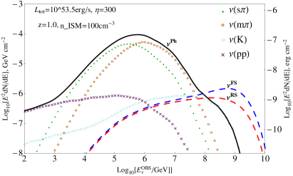
Figure 3: The observer frame $\nu_{\mu}+\bar{\nu}_{\mu}$ fluence $E^{2}dN/dE$ for a $\mu=1/3$ magnetically dominated burst at $z=1$. Solid line($\nu^{\rm Ph}$): total muon neutrino spectrum from $\Delta$-resonance (dotted), $p\gamma$ multi-pion production (circle), $pp$ collision (cross) and Kaons(square). Large dashed line ($\nu^{RS}$ and $\nu^{FS}$): total neutrino spectrum from external reverse and forward shock in the early afterglow. For the forward shock neutrino calculation, we included the photons from the reverse shock as well.

Fig.3, as well as Fig.4,5 also illustrate the effect on the neutrino spectra of including additional physical processes besides the $p\gamma$ production from the $\Delta^{+}$-resonance used in many previous studies, including the recent IceCube GRB data analyses (Abbasi et al., 2012). The processes included in Figs.3, 4 and the rest are the production of $\pi^{\pm}$ via $\Delta^{+}$ in $pp$ as well as $p\gamma$, as well as multi-pion production and $K^{\pm}$ in $pp$ and $p\gamma$. We note that $pp$ collisions can become important at lower energies (before $p\gamma$ interactions set in). This is especially true if the dissipation radius $R_{\rm dis}$ is small, where the $pp$ collision optical depth $\tau_{pp}$ approaches unity or above. We also note that the neutrino fluence is comparable to the photon fluence in fig.1. This may be a relatively conservative value; in some other works a higher acceleration efficiency , pionization efficiency and proton luminosity e.g $L_{p}=10L_{\gamma}$ are adopted corresponding to a neutrino luminosity $L_{\nu}\sim$ a few ${L_{\gamma}}$.

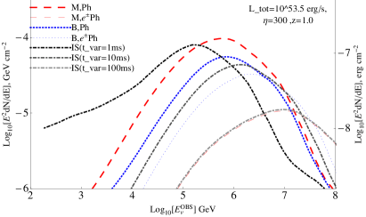
Figure 4: The $\nu_{\mu}+\bar{\nu}_{\mu}$ fluence spectra for different models assuming a source at redshift $z=1$. $L_{\rm tot}=10^{53.5}$ erg/s, $\eta=300$ are used. (External shock neutrino spectrum is not calculated here.) The models shown here are the $\mu=1/3$ magnetic photosphere (M,Ph), $\mu=1$ baryonic photosphere (B,Ph) , pair-photosphere dissipation (M,$e^{\pm}{\rm Ph}$ or M,$e^{\pm}{\rm Ph}$) and internal shock shock models (IS) with $t_{\rm var}=1,10,100$ ms (black, dark gray, light gray)

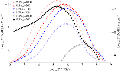
Figure 5: The neutrino spectrum from a magnetic photosphere (red upstanding triangle), a baryonic photosphere (blue inverted triangle) and an internal shock model (black square), for $\eta=300$ (filled) $\eta=1000$ (empty). Both the two lines for internal shock models have used $t_{\rm var}=1$ ms. The other parameters are the same as in fig.4. Note that a slower jet produces a higher neutrino flux in all these cases. The more detailed quantities for those models (and in fig.4) are listed in Table.1.

In Fig.4, we also show the possible effect of having a dissipative photosphere at a radius larger than that given by Eqn.(5), e.g. due to pair effects. Without specifiyng an underlying mechanism giving rise to the dissipation and Band function spectrum this increase is uncertain. If the photon spectrum is generated by the scattering of thermal electrons associated with turbulent Alfven waves (Thompson, 1994), the maximum energy of the comoving photons can hardly exceed the electron rest mass $m_{e}c^{2}$ and negligible pairs are produced. On the other hand if the prompt emission is due to synchrotron radiation from Fermi-I accelerated electrons e.g. (Drury, 2012) and the attenuation beyond $E_{\rm max}^{\prime}$ is due to $\gamma\gamma\to e^{+}e^{-}$ process, we can calculate $\tau_{\gamma\gamma}$ and the amount of pairs. The existence of pairs with such parameters (Fig.1) could boost the pair-photosphere radius to $\sim 20$ times the original $R_{\rm ph}$. In the collisional scenario where protons and neutrons decouple (Beloborodov, 2010), high energy $\gamma$s and injected poisitrons from decaying pions induce leptonic cascades and significant pair production, which gives a similar boost of $\sim 20$ to a pair-photosphere radius. Without going into specific model details, we just consider for simplicity the dissipative and spectrum formation effects associated with such larger effective pair photospheres, and use this radius for calculating the neutrino spectrum. In Fig.4 the curve labelled ${\rm M},e^{\pm}{\rm Ph}$ is for a magnetized dynamics photosphere a factor $\sim 20$ larger, and the curve labelled ${\rm B},e^{\pm}{\rm Ph}$ is for a baryonic photosphere a factor $\sim 3.6$ larger than the value of Eqn.(5).

The case of an internal shock is also shown, for a dissipation radius estimated by Eqn.24 and variability time $t_{\rm var}=1$ ms. Qualitatively, the harder spectra from larger radius dissipation regions arise because the magnetic field and photon density is lower at larger radii, reducing the pion and muon electromagnetic cooling.

The effect of a magnetic versus a baryonic jet bulk dynamics on the neutrino signatures are compared in Fig.5, where we plot the neutrino spectra from a magnetic photosphere where $\Gamma\propto{r^{1/3}}$, a baryonic photosphere where $\Gamma\propto{r}$ and an internal shock model. Each case is calculated for two different terminal Lorentz factors, $\eta=300$ and $\eta=1000$.

The neutrino fluence in general decreases for increasing $\eta$ in the baryonic photosphere model. The analytical expression for the photospheric radius is $R\propto\eta^{-3}$ in this model (Eqn.5), and having assumed a fixed Band function in the comoving frame, the number density of target photons is $n_{ph}^{\prime}\sim{u_{ph}^{\prime}/E^{\prime}\Delta{E}^{\prime}}\propto L/R^{2}\eta^{2}\propto\eta^{4}$. Therefore, the $p\gamma$ inverse cooling timescale $t_{p\gamma}^{\prime{-1}}\propto{n_{ph}^{\prime}}\propto\eta^{4}$ We also have $t_{dyn}^{\prime{-1}}\sim\eta{c}/R\sim\eta^{4}\sim{t}_{ad}^{\prime{-1}}$. The pionization efficiency $f_{\pi}=t_{p\gamma}^{\prime{-1}}/t_{ad}^{\prime{-1}}$ has no dependence on $\eta$ in the leading order approximation, or on $R$, which is treated as a function of $\eta$ here. But, the synchrotron cooling for $\pi^{\pm}$, $\mu^{\pm}$ ($t_{\rm sync}/t_{\rm dec}\propto\eta^{-4}$ for given $\pi,\mu$ energy) diminishes the neutrino flux for larger $\eta$. . From Fig.5 we see that the peak energy of $\eta=1000$ is smaller than $\eta=300$ case in the comoving frame. This indicates strong pion cooling taking place. Therefore a higher $\eta$ is associated with a smaller $\nu$ flux.

For the magnetic photosphere, a larger $\eta$ gives smaller $R_{\rm ph}$ and $\Gamma_{\rm ph}$. Both are advantageous for neutrino production (although a higher magnetic field lead to stronger cooling of pions and muons, it is less severe than the baryonic case, e.g. see $B_{5}@R$ column in Table.1).

In Fig.6, upper panel, we compare the luminosity dependence of the single source spectra for a standard $\eta=300$ of an “optimistic" internal shock model (with a high dissipation rate and $t_{\rm var}=1,~{}10,~{}100$ ms), a magnetic photosphere model and a baryonic photosphere model. The optimistic internal shock model with $t_{\rm var}=1$ ms gives the highest flux at energies $\lesssim 100$ TeV, while the magnetic photosphere models have a lower flux at these energies, with their spectrum also peaking towards higher energies. In Fig.7 upper panel we show those cases with $\eta=1000$. We see that the magnetic photosphere case is the least affected by $\eta$.

An interesting possibility in the case of magnetic dissipation regions, e.g. due to reconnection, is that they may produce an an accelerated proton spectrum which is harder than the typical Fermi case of $dN/dE\propto{E^{-2}}$. As discussed by (Drury, 2012; Bosch-Ramon, 2012) for an extreme case all the protons entering the acceleration process are essentially confined by the magnetic field and the zero escape probability leads to a spectrum $dN/dE\propto{E^{-1}}$. If this scenario is valid, the bulk of the energy for the accelerated protons is concentrated in the high energy end of their injection spectrum. The neutrino energy associated with these protons lies in the PeV-EeV energy range. This energy is in the sensitivity range of IceCube and proposed ARIANNA neutrino detector. However this scenario requires significant magnetic reconnection process where the toroidal magnetic field is still present. Charged pions and muons at this energy suffer strong synchrotron cooling which suppresses the neutrino spectrum significantly. Therefore, no significant neutrino emission is expected from this scenario (since at lower energies there are too few protons due to the nature of a $dN/dE\propto{E^{-1}}$ spectrum.)

V Diffuse neutrino background from various GRB models and implications

Since the individual source fluxes are very low, except for the unlikely event of an extremely nearby occurrence, it is useful to consider the cumulative diffuse neutrino flux from all GRBs in the sky. We calculate this diffuse flux based on two methods. Method-I uses a GRB luminosity distribution (luminosity function) and a redshift distribution (Wanderman and Piran, 2010), given, respectively, by

$$\phi(L_{\gamma})\propto\begin{cases}(L_{\gamma}/L_{*})^{m_{1}}&L_{\rm min}<L_{\gamma}<L_{*}\\ (L_{\gamma}/L_{*})^{m_{2}}&L_{*}<L_{\gamma}<L_{\rm max}\end{cases}$$ (26)

$$R_{\rm GRB}(z)\propto\begin{cases}(1+z)^{n_{1}}&z<z_{1}\\ (1+z)^{n_{2}}&z>z_{1}\end{cases}$$ (27)

Here $L_{\gamma}$ is the peak photon luminosity (here mostly in the 0.1-1 MeV range) and we have used the following values: $L_{\rm min}=10^{50}$ erg/s, $L_{*}=10^{52.5}$ erg/s , $L_{\rm max}=10^{54}$ erg/s, $m_{1}=-0.17$ , $m_{2}=-1.44$ , $n_{1}=2.07$ , $n_{2}=-1.36$ , $z_{1}=3.1$ which are best fit values used in (Wanderman and Piran, 2010). The differential comoving rate of GRBs at a redshift $z$ is

$$R(z)=\frac{R_{\rm GRB}(z)}{(1+z)}\frac{dV}{dz}$$ (28)

where V(z) is the comoving volume in the standard ${\rm\Lambda{CDM}}$ cosmology given by parameters in Eqn.25 and the factor (1+z) accounts for time dilation effect due to cosmic expansion. The differential number of GRB per unit redshift is given by

$${\rm d}N(L_{\gamma},z)=\rho_{0}\phi(L_{\gamma})R(z){\rm d}{\log}L_{\gamma}{\rm d}z$$ (29)

where $\rho_{0}=1.3{\rm/yr/Gpc^{3}}$ is the local rate of high luminosity GRBs (not including a separate family of objects called low luminosity GRBs (Liang et al., 2007)).

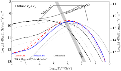
Figure 6: Upper panel: Neutrino fluence from a single GRB from different dissipation regions. Red, dashed: magnetic photosphere; blue, dotted: baryonic photosphere; Dot-dash: baryonic internal shock for $t_{\rm var}=1,10,100$ ms. (black, dark gray, light gray). These are computed for different luminosities (in each model, $L_{\gamma}=10^{53},10^{52},10^{51}$ erg/s (top,middle,bottom). Lower panel: Diffuse $\nu_{\mu}+\bar{\nu}_{\mu}$ neutrino spectral flux from the three models above (same line style), calculated for an all-sky GRB rate of 700/yr using statistical Method I (thick lines) and Method II (thin lines; see §V). Also shown is the IceCube collaboration’s representation of the diffuse flux from a standard Waxman-Bahcall internal shock model, and the IC 40+59 observational upper limit (see Fig.3 of (Abbasi et al., 2012) for description). The gray zone labeled ATM is the atmospheric neutrino spectrum. The plots from both panels suggest that the occasional electromagnetically bright GRBs can contribute significantly to the total diffuse flux.

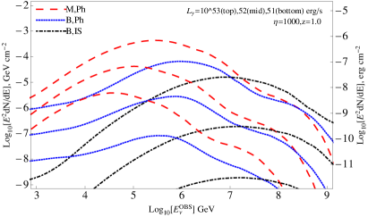
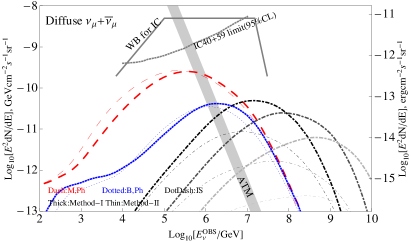
Figure 7: The parameters and conventions are the same as those in fig.6 except we have used $\eta=1000$ (in fig.6,$\eta=300$ is used).

An alternative method (Method-II) is to use the Wisconsin GRB catalog [http://grbweb.icecube.wisc.edu/]. We consider only long GRBs and use the parameters such as the Band photon index, fluence, redshift, photon peak energy etc. to compute the neutrino spectrum from each individual burst and stack them together. Finally we normalize the resultant flux to an all sky rate of 700 GRBs/yr. These two methods are then used to calculate the diffuse neutrino flux assuming that the GRB neutrinos are due to a magnetic photosphere, a baryonic photosphere, and an internal shock model (Fig.6,7). In Fig.6 we plot those cases with $\eta=300$ while in Fig.7 $\eta=1000$.

An inspection of this Fig.6,7 (lower panel) shows that the above models, with the parameters used in this paper, predict a diffuse neutrino flux which is likely to be within the current constraints set by IceCube 40+59 string observations, as suggested by the fact that they lie below the two IceCube constraint lines labeled WB for IC and IC 40+59. A caveat is that these constraints are upper limits on the flux as a function of the break energy assuming a Band function with $\alpha=-1,\beta=-2$, or assuming a slope -2. They are not directly applicable to other types of spectra; thus, these constraint lines are here intended only for a rough comparison; they would have to be re-evaluated for the spectra shown here. Nonetheless, they do provide some guidance, and it appears that the only models which are close to being constrained at present are those using the most optimistic parameters; e.g. for internal shock models with a $t_{\rm var}=1$ ms one would expect a small dissipation radius leading to a high $\tau_{\rm pp}$ and a high neutrino fluence in the lower energy range from $pp$ collisions (where $\tau_{\rm p\gamma}$ has saturated to unity with $\tau_{\rm pp}$ increasing, making $pp$ collisions more important.) Also, if we were to assume a higher value of $\epsilon_{p}/\epsilon_{e}$, such as 10 (in this paper we used a value of $1$, see also section. IV) and/or if we were to adopt a lower magnetic field fraction ($\epsilon_{B}\simeq 10^{-2}$, rather than the $\epsilon_{d}\epsilon_{B}=0.1$ used here), the diffuse neutrino fluence would be likely to violate the above constraints, especially for the internal shock model. However, this is for the optimistic internal shock case where one uses $t_{\rm var}=1$ ms, whereas there is a larger uncertainty in this quantity, and in most bursts $t_{\rm var}$ can often be several orders or magnitude larger (see comments in the third paragraph of §IV). For such larger (and more reasonable) values of $t_{\rm var}$ the model would appear to be still compatible with the constraints, even if a high $\epsilon_{p}/\epsilon_{e}$ ratio were assumed.

We have also included the approximate atmospheric neutrino background in Fig.6,7. It is worth noting that GRBs are transient sources whose prompt emission duration in the observer frame is within $t_{\rm dur}^{\rm obs}\sim 100$ s. The angular resolution for TeV neutrino and above is within $1~{}{\rm deg^{2}}$. Therefore, considering the search time bin and the small solid angle set by optical observations, the effective atmospheric neutrino background is well below these GRB diffuse fluxes. In other words, even one or two muon events in IceCube correlated with photon detections would give a high signal to noise ratio.

A caveat for such calculations of the diffuse background is that the statistical description of both the source physics parameters and the spatial-temporal distribution of the sources has large uncertainties; this applies to both the luminosity function (Method I) and the observed burst catalog (Method II). In Method-I, the parameters in eqns. (26, 27) have large uncertainties; especially in the low redshift region (e.g. $z<0.3$), very few GRBs are observed. However, in order to expect more than one muon event in IceCube, we need a GRB of moderate or high luminosity located at low redshift (such as the example GRB in fig.4 with $L_{\gamma}=10^{52.5}$ erg/s and $z=0.1$, which results in about 0.2 muon events in the IceCube 86-string configuration.) The estimated rate of GRBs which satisfy $N_{\rm\mu,Icecube}\geq{1}$ is about $o(1)$ per ten years. In Method-II, we actually have a very limited number of GRBs with well measured redshifts in the catalog. Those without a redshift are assigned a default redshift value of $z=2.0$. Thus, improvements in the photon-based statistics of bursts, as well as neutrino observations over multi-year periods appear required.

VI Discussion

We have calculated the $\nu_{\mu}+{\bar{\nu}}_{\mu}$ signatures expected from photospheric GRB models where the dynamics is either magnetically or baryonically dominated, including also the effects of external shocks, and have compared these signatures with those expected from the baryonic internal shock models. This comparison is timely in view of recent developments, the most pressing being the recently published IceCube constraints (Abbasi et al., 2011, 2012) on the “standard" internal shock GRB models. The exploration of alternative models to the internal shocks has its own separate motivation, independently of the IceCube observations. One reason is the increased realization that magnetic fields may play a dominant role in the GRB phenomenon, and the dynamics of magnetically dominated GRB jet models are being considered in detail (Drenkhahn and Spruit, 2002; Tchekhovskoy et al., 2010; McKinney and Uzdensky, 2012). Also, issues related to the efficiency and spectrum of standard internal shock models of the prompt $\gamma$-ray emission (Preece et al., 2000; Medvedev et al., 2004; Meszaros, 2006) have led, on the one hand, to considering modified internal shock models that address these issues, e.g.(Asano and Mészáros, 2011; Inoue et al., 2011; Murase et al., 2012), etc., and, on the other hand, to considering the photospheric emission as the source of the prompt $\gamma$-rays, including both baryonic photospheres (Mészáros and Rees, 2000; Ryde, 2005; Rees and Mészáros, 2005; Pe’er et al., 2006; Beloborodov, 2010; Pe’er, 2011) and magnetic photospheres (Giannios and Spruit, 2007; Mészáros and Rees, 2011b; Veres and Mészáros, 2012). Some previous calculations of neutrino spectra from baryonically dominated photospheres have been carried out (Murase, 2008; Wang and Dai, 2009), but so far none from dissipative photospheres or magnetic photospheres, which we treat here

One of the notable features about the neutrino emission from dissipative photosphere models, both in magnetized of baryonic dynamics, is that the peak energy of the spectrum (which is around 0.5-1 PeV, as seen in Fig. 3) differs from the peak energies of a typical Waxman-Bahcall (WB97)(Waxman and Bahcall, 1997) simplified standard internal shock model such as used in the recent IceCube studies (and in (Guetta et al., 2001a, 2004)). The peak energy is also higher than those for the internal shock model with $t_{\rm var}=1{\rm ms}$ and $\eta=300$, but lower than those with higher $t_{\rm var}$ and $\eta$ values. In part, this is due to the inclusion, in addition to $\Delta$ resonance production, also of multi-pion effects, Kaon decay, etc., which also gives a steeper spectrum above the peak, compared to the flat slope of $E^{2}dN/dE$ above the peak expected in the usual WB97 internal shock model. This steepening of the spectrum above the peak is not unique to the photospheric dissipation model, it occurs also in internal shocks when we include the above additional physics beyond the $\Delta$-resonance, as can be seen in Fig. 4. (Such a steepening for internal shocks is also found by (Hümmer et al., 2012)).

The energy at which the spectral peak appears depends generically on the radius of the dissipative and photon escape zones, which here we have assumed to be colocated, whether it be a photosphere or an internal shock. The effect of different radii is illustrated in Fig. 4, which compares the spectra and peak energies of different photospheric dissipation zones at different radii and also two internal shocks at two different radii (or variability times). The harder spectra from larger radii are expected because of the decrease of the magnetic fields and and photon densities, which allows the higher energy secondary pions and muons to decay before significant electromagnetic cooling has taken place.

The difference between a magnetically dominated photosphere (M,Ph), a baryonically dominated photosphere (B,Ph) and internal shock (IS) models are compared in Fig.4,5, Fig.6,7(upper panel) and Table.1. The dissipation region for the ‘M,Ph’ typically lies in the acceleration phase of the jet where there is a smaller $\Gamma_{\rm ph}$ than ‘B,Ph’ and ‘IS’ model. The neutrino spectrum in the observer frame is affected by the efficiency of $pp$ and $p\gamma$ interaction, the cooling of the secondary charged particles (which is mainly synchrotron, determined by the comoving magnetic field) and finally Lorentz boost and redshift. The differences in neutrino spectra from these models are not quite significant for $\eta=300$ where the dissipation region, magnetic field and Lorentz factor are similar. For $\eta=1000$, the ‘B,Ph’ and ‘IS’ have harder spectra than the ‘M,Ph’ model. The ‘B,Ph’ radius here is rather small where $pp$, $p\gamma$ and coolings are all efficient. The large Lorentz boost factor finally pushes the peak neutrino energy in the observer frame over the ‘M,Ph’ model. For ‘IS’ model with $\eta=1000$ the dissipation radii is much larger than ‘M,Ph’ and ‘B,Ph’ case. The inefficient cooling results in the highest peak energy of the three models. However, the flux is also the lowest because $pp$ and $p\gamma$ are the least efficient of these models.

The maximum source-frame energy of the accelerated protons which are able to escape the acceleration region, for the models considered here, are shown in the third from the last column of Table.1. Leaving out any consideration of the diffuse flux, it is seen that only the internal shock models approach the highest energies associated with the GZK limit, as originally suggested by (Waxman and Bahcall, 1997), while all photospheric models fall several orders of magnitude below this energy. We have not done an exhaustive parameter search, since our emphasis has been the neutrino emission, but it is apparent that photospheric models would not be competitive GZK sources.

The detection of neutrinos from individual single sources with the 86 string IceCube, as seen from Table.1 in the last two columns, is rather difficult, the number of expected muon events at best being $\sim 0.2$ for a magnetic photosphere model of average luminosity at $z=0.1$. The only hope may be the statistically rare observation of a nearby bright GRB , or through observations of the diffuse flux.

The diffuse flux offers higher prospects for an eventual detection, and a comparison of the diffuse flux expected from the three different types of models discussed, Figs. 6 and 7 lower panels, shows that an internal shock scenario with optimistic parameters such as $t_{\rm var}=1{\rm ms}$ and $\eta=300$ comes closest to being constrained by the current IceCube limits (Abbasi et al., 2012). This confirms the recent calculations of (Li, 2012; He et al., 2012; Hümmer et al., 2012). On the other hand, a magnetic photosphere model is far from being constrained by the current limits (although the limits will have to be re-evaluated for the specific spectral shapes). A baryonic dissipative photosphere model has an even lower flux, and would take the longest to be detected. Fig.7 shows that a higher Lorentz factor, in this case $\eta=1000$, decreases the constraints. The diffuse flux from a magnetic photosphere is the least affected, and both baryonic photosphere and internal shock models have higher peak energy but lower flux.

In conclusion, the calculations discussed in the previous sections indicate that the current IceCube limits are not yet sufficient to distinguish between the dissipative photosheric models based on magnetic or baryonic dynamics, although they are approaching meaningful limits for baryonic internal shocks outside the photospheres. Also, as of now it is not yet possible to set stringent limits on the value of $\epsilon_{p}/\epsilon_{e}$, i.e. the putative ration of accelerated protons to accelerated electrons. One of the reasons, for the photospheric models, is that the magnetic reconnection or dissipation scenario is less straightforward than the simple internal shock scenario, having both more physical model uncertainties and parameters associated with them, e.g. the geometry of the plasma layers or the striped field structures, resistivity, instabilities, reconnection rate, etc. Both for photospheric and internal shock models, the fraction of protons that are injected into the reconnection or Fermi acceleration process is uncertain. The acceleration timescale and escape probability depend on the geometry and dynamics of magnetic reconnection or acceleration region. These factors are also crucial for determining the injection of a cosmic ray proton spectrum and its effect on the neutrino fluence, maximum neutrino energy and spectrum.

For these reasons, and in preparation for future improved limits from longer observation times and from possible future higher sensitivity detectors, we have here investigated the typical neutrino spectral features and flux levels expected from three of the basic GRB models currently being considered. There are reasonable prospects that the detection or non-detection of these neutrino fluxes in the next decade with IceCube or next generation of large neutrino detectors will shed light on the underlying physics of the GRB jets and on the cosmic ray acceleration process in then.