Evolution of isolated overdensities as a control on cosmological N body simulations

Abstract

Beyond convergence studies and comparison of different codes, there are essentially no controls on the accuracy in the non-linear regime of cosmological N body simulations, even in the dissipationless limit. We propose and explore here a simple test which has not been previously employed: when cosmological codes are used to simulate an isolated overdensity, they should reproduce, in physical coordinates, those obtained in open boundary conditions without expansion. In particular, the desired collisionless nature of the simulations can be probed by testing for stability in physical coordinates of virialized equilibria. We investigate and illustrate the test using a suite of simulations in an Einstein de Sitter cosmology from initial conditions which rapidly settle to virial equilibrium. We find that the criterion of stable clustering allows one to determine, for given particle number $N$ in the “halo” and force smoothing $\varepsilon$, a maximum red-shift range over which the collisionless limit may be represented with desired accuracy. We also compare our results to the so-called Layzer Irvine test, showing that it provides a weaker, but very useful, tool to constrain the choice of numerical parameters. Finally we outline in some detail how these methods could be employed to test the choice of the numerical parameters used in a cosmological simulation.

1 introduction

Numerical simulations of structure formation in the universe in cosmology use the $N$ body method in which the continuum density field of dark matter is represented by a finite number of discrete particles interacting by a smoothed Newtonian two body potential. It is evidently of importance to control as much as possible for their precision and reliability. Specifically, beyond issues of numerical convergence, it is important to understand the limits imposed on the accuracy of results by the use of a finite number of particles to represent the theoretical continuum density field, and the associated introduction of a smoothing scale (or equivalent) in the gravitational force. This latter scale, $\varepsilon$, clearly imposes a lower limit on the spatial resolution, so in order to optimize resolution the question is how small a value of $\varepsilon$ may be employed for a given number of particles and starting redshift. This question has been the subject of some controversy, notably concerning whether values of $\varepsilon$ smaller than the initial inter-particle distance may be employed (see e.g. Splinter et al. (1998); Knebe et al. (2000); Power et al. (2003); Heitmann et al. (2005); Joyce et al. (2008); Romeo et al. (2008)).

In this article we discuss one way in which cosmological N body codes may be tested for their reliability which has not been explored previously. The idea is based on the simple observation that, applied to the simulation of an “isolated” overdensity (i.e. a finite system of size much smaller than that of the periodic simulation box), a cosmological simulation should be equivalent, in physical coordinates, to one performed in open boundary conditions without cosmological expansion. Indeed the only differences between the two should arise from possible differences in the force smoothing and finite size effects, both of which are variables on which the physical results of a cosmological simulation should not depend. Even without a direct comparison with simulations in open boundary conditions, the desired collisionless nature of cosmological simulations can be tested for by probing whether an isolated virialized structure, corresponding to a collisionless equilibrium, remains stable in physical coordinates.

By “isolated” we mean that there is no other mass in the periodic box other than the structure considered, which itself evolves in a region of a size small compared to that of the box. The structure is therefore isolated but for the interaction with its “copies” included in the infinite system over which the force is summed. We illustrate with a set of numerical simulations how this required equivalence of the evolution in codes with and without expansion can be used to actually determine whether a given choice of numerical parameters for cosmological simulations is appropriate. We focus in particular on the choice of the smoothing length in the force, and show that the test allows one to determine a range of appropriate values.

To avoid possible confusion it is probably useful to underline the distinction between stable clustering as we study it here, and the same term as it is frequently discussed in cosmological simulations (see, e.g., Efstathiou et al. (1988); Smith et al. (2003)): it can be postulated (Peebles, 1980) that, in the strongly non-linear regime, structures evolve as if they were isolated from the rest of the mass in the universe. If this “stable clustering hypothesis” is valid (to a good approximation, on average) it leads, when matched with linear theory, to very specific predictions for the nature of the correlations in the non-linear regime. Here, in contrast, we will consider by construction the evolution only of a single structure, for which stable clustering must be observed if the simulation is reproducing the desired physical limit.

The article is organized as follows. In the next section we show explicitly how cosmological codes used to simulate isolated overdensities in an expanding universe are related, in an appropriate limit, to non-expanding codes. We then discuss the particular limit of virialized halos, for which the stationarity in a non-expanding code corresponds to stable clustering in physical coordinates in the expanding code. In the following section we illustrate and investigate the test using a set of simulations in an Einstein de Sitter (EdS) universe, which differ only in the smoothing length employed. We then also consider a set of simulations in which only the box size is varied. In the subsequent section we compare the test with the so-called Layzer Irvine test for the evolution of the energy in cosmological simulations. In Sect. 5 we discuss what can be inferred from our results about the role of different possible discreteness effects in producing the observed deviations from stable clustering, and what can be concluded about dependences of these deviations on the relevant parameters (particle number, force smoothing, box size). In the following section we specify in a “recipe” form how the test could be employed practically by simulators to test choice of numerical parameters in cosmological simulations. We conclude with a brief discussion of possible variants on the tests and some more general comments.

2 Evolution of an isolated overdensity in cosmological N body codes

Dissipationless cosmological N-body simulations (see, e.g., Kravtsov et al. (1997); Springel et al. (2001); Teyssier (2002), or Bagla (2005) for a review) solve numerically the equations

$$\frac{d^{2}{\bf x}_{i}}{dt^{2}}+2H\frac{d{\bf x}_{i}}{dt}=\frac{1}{a^{3}}{\mathbf{F}}_{i}$$ (1)

where

$${\mathbf{F}}_{i}=-Gm\sum_{j\neq i}^{P}\frac{{\bf x}_{i}-{\bf x}_{j}}{|{\bf x}_{i}-{\bf x}_{j}|^{3}}W_{\varepsilon}(|{\bf x}_{i}-{\bf x}_{j}|)\,.$$ (2)

${\bf x}_{i}$ are the comoving particle coordinates of the $i=1...N$ particles of equal mass $m$, enclosed in a cubic box of side $L$, and subject to periodic boundary conditions, $a(t)$ is the appropriate scale factor for the cosmology considered, and $H(t)={\dot{a}}/{a}$ is the Hubble constant. The function $W_{\varepsilon}$ is a regularisation of the divergence of the force at zero separation — below a characteristic scale, $\varepsilon$, which is typically fixed in comoving units. For simplicity we will drop this function in this section as it plays no role for our considerations here.

The superscript ‘P’ in the sum in (2) indicates that it runs over the infinite periodic system, i.e., the force on a particle is that due to the $N-1$ other particles and all their copies. The sum, as written, is formally divergent, but it is implicitly regularized by the subtraction of the contribution of the mean mass density. This is physically appropriate, in an expanding universe, as the mean mass density sources the expansion (see e.g. Peebles (1980)).

2.1 Equations of motion a single “isolated” structure in physical coordinates

Let us now consider the case illustrated schematically in Fig.1 where the $N$ particles are contained within a spherical volume, $\Omega$, of radius $R$, with $R<L/4$ (where $L$ is the side of the cube). The latter condition is sufficient to ensure that the distance between any particle $i$ and any other particle $j$ in $\Omega$ is less than that separating $i$ from any copy of $j$ in the infinite periodic system. The force on a particle $i$ may then be written

Figure 1: Schematic representation of the case studied in this paper: a single structure of $N$ particles confined in a region of characteristic size small compared to the side of the cubic cosmological simulation box (dark line).

$${\mathbf{F}}_{i}={\mathbf{F}}_{i}^{\Omega}+{\mathbf{F}}_{i}^{c}$$ (3)

where

$${\mathbf{F}}_{i}^{\Omega}=-Gm\sum_{j\neq i}\frac{{\bf x}_{i}-{\bf x}_{j}}{|{\bf x}_{i}-{\bf x}_{j}|^{3}}$$ (4)

is simply the direct one over the $N-1$ other particles in the volume $\Omega$, and

$${\mathbf{F}}_{i}^{c}=\sum_{j\neq i}{\mathbf{F}}_{ij}^{c}=-Gm\sum_{j\neq i}\sum_{{\bf n}\neq 0}\frac{{\bf x}_{i}-{\bf x}_{j}-{\bf n}L}{|{\bf x}_{i}-{\bf x}_{j}-{\bf n}L|^{3}}$$ (5)

is the force due to all the particles in the copies, labelled by all vectors of non-zero integers ${\bf n}$, and where we have $|{\bf x}_{i}-{\bf x}_{j}|<L/2<|{\bf n}L|$. Note that ${\mathbf{F}}_{i}^{\Omega}$ is clearly finite and well defined, while each sum over ${\bf n}$ giving ${\mathbf{F}}_{ij}^{c}$ is now formally divergent, but again implicitly regulated by the subtraction of the mean density.

To calculate ${\mathbf{F}}_{ij}^{c}$ we observe that it corresponds simply to the force on a single particle displaced by $({\bf x}_{i}-{\bf x}_{j})$ off an infinite perfect lattice of lattice spacing $L$. It is straightforward to show (see Gabrielli et al. (2006)) that, expanding in Taylor series in $({\bf x}_{i}-{\bf x}_{j})$ about ${\bf x}_{i}-{\bf x}_{j}=0$, we have

$${\mathbf{F}}_{ij}^{c}=\frac{4\pi G\rho_{0}}{3N}({\bf x}_{i}-{\bf x}_{j})+O(|{\bf x}_{i}-{\bf x}_{j}|^{2}/L^{4})$$ (6)

where $\rho_{0}=mN/L^{3}$ is the total mean mass density (and thus $\rho_{0}/N$ the mean mass density of the lattice of the particle $j$ and its copies). The leading non-zero “dipole” term on the right hand side in (6) is a repulsive term which arises from the subtraction of the mean mass density to regulate the sum: it is precisely the force arising from the mass contained in a sphere of radius $|{\bf x}_{i}-{\bf x}_{j}|$ of constant mass density $-\rho_{0}/N$. We do not write explicitly the sums for the subsequent (quadrupole and higher multipole) terms, but they are manifestly convergent and suppressed by positive powers of $(R/L)$ compared to the dipole term.

As the sum over ${\bf x}_{j}$ in ${\mathbf{F}}_{i}^{c}$ vanishes because we have chosen (without loss of generality) to place the center of mass of the $N$ particles in $\Omega$ at the origin of our coordinates, retaining only the dipole term in ${\mathbf{F}}_{i}^{c}$ the equations of motion (1) we obtain

$$\frac{d^{2}{\bf x}_{i}}{dt^{2}}+2H\frac{d{\bf x}_{i}}{dt}=-\frac{Gm}{a^{3}}\sum_{j\neq i}\frac{{\bf x}_{i}-{\bf x}_{j}}{|{\bf x}_{i}-{\bf x}_{j}|^{3}}+\frac{4\pi G\rho_{0}}{3}{\bf x}_{i}$$ (7)

where the sum is now only over the $N-1$ particles in $\Omega$. Assuming an EdS cosmology, for which

$$\frac{\ddot{a}}{a}=-\frac{4\pi G\rho_{0}}{3a^{3}}\,,$$ (8)

these equations (2) may be written, in physical coordinates ${\bf r}_{i}\equiv a(t){\bf x}_{i}$, simply as

$$\frac{d^{2}{\bf r}_{i}}{dt^{2}}=-Gm\sum_{j\neq i}\frac{{\bf r}_{i}-{\bf r}_{j}}{|{\bf r}_{i}-{\bf r}_{j}|^{3}}$$ (9)

i.e. as the equations of motion of $N$ isolated purely self-gravitating particles .

Thus, when a cosmological code is used to simulate an isolated structure in an expanding universe, it should reproduce the same result, in physical coordinates, as that obtained for such a structure in open boundary conditions without expansion. This identity is valid up to

• finite size corrections, arising from the use of a finite (periodic) box in cosmological simulations (and which vanish in the limit $R/L\rightarrow\infty$).

• eventual differences due to force softening in the two type of codes (which we have neglected above).

Any dependence of results on the box size or force smoothing is unphysical in cosmological codes. Thus these codes can be tested by using them to simulate isolated structures and comparing the results obtained to those for the same initial conditions in open boundary conditions and without expansion.

2.2 Virialization and stable clustering

Results for the detailed evolution from arbitrary initial conditions in open boundary conditions and without expansion can be obtained in general only from numerical simulation. However, even without performing such simulations, it is possible to do tests of cosmological codes which are based on well established generic features of the evolution in open boundary conditions. One such feature, for a very wide class of simple initial conditions, is the evolution to a virial equilibrium in a few dynamical times (see e.g. Heggie & Hut (2003)). These equilibria are, in the limit $N\rightarrow\infty$, stationary states corresponding to time independent solutions of the collisionless Boltzmann equation. In a finite $N$ system they evolve away from this equilibrium, on a very long time scale diverging with $N$, due to collisional effects. The stationarity of these states in the collisionless limit corresponds, in a cosmological code, to “stable clustering” of the virialized system.

It follows that by studying the stability of the evolution obtained from appropriate initial conditions, we can test cosmological codes both for effects arising from the finite size of the box, and force smoothing, as well as for collisional effects. These are precisely the principle undesired effects introduced by using the N-body method to solve the (continuum, infinite system) cosmological problem of formation of structure, and present even in the idealized limit that the numerical integration of the equations of motion is arbitrarily accurate. Thus by testing for the validity of stable clustering in such a regime we can test for the capacity of N body codes to reproduce correctly the relevant physical limit. It is such a test which we will focus on in what follows.

3 Numerical study of the test

To illustrate the test we use the GADGET code   (Springel et al., 2005), which can be used to perform both cosmological simulations, and simulations without expansion (in both open and periodic boundary conditions). For our cosmological simulations we consider, for simplicity, evolution in an Einstein de Sitter background. All our simulations here are for $N=10^{4}$ particles.

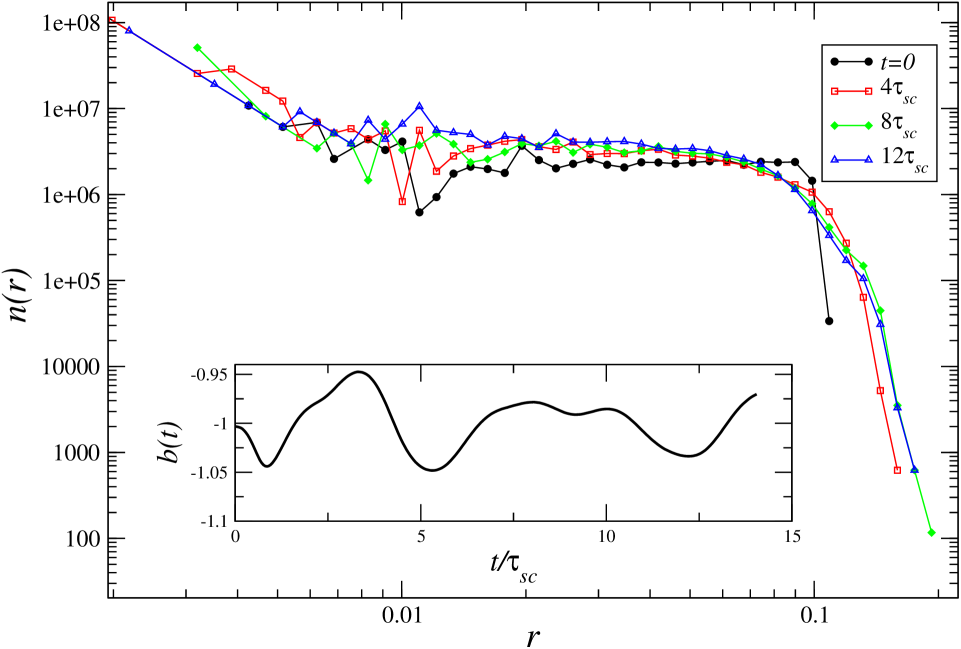
Figure 2: Density profile (and, inset, virial ratio) at indicated times for our chosen initial conditions when evolved in open boundary conditions (and without expansion).

3.1 Initial conditions and choice of units

The initial conditions we study here are the following: the $N=10^{4}$ particles are randomly distributed in a spherical volume of radius $R=0.1L$, and assigned random velocities sampled from a probability distribution which is uniform in a cube centered at zero velocity. These velocities are then normalized so that $b=-1$, where

$$b=\frac{2K_{p}}{U_{p}}$$ (10)

is the virial ratio, and $K_{p}$ and $U_{p}$ are the peculiar kinetic energy and peculiar potential energy respectively. These are defined by

$$K_{p}=\frac{1}{2}\sum_{i}m|\vec{v}_{i}|^{2}$$ (11)

where $\vec{v_{i}}=a(t)\frac{d\vec{x}_{i}}{dt}$ is the particle peculiar velocity, i.e.,

$$\vec{v}_{i}=a(t)\frac{d\vec{x}_{i}}{dt}=\frac{d\vec{r}_{i}}{dt}-H(t)\vec{r}_{i}$$ (12)

and

$$U_{p}=\frac{1}{2a}\sum_{i,j,i\neq j}mg(|\vec{x_{i}}-\vec{x_{j}}|)$$ (13)

where $g(r)$ is the exact (GADGET) two body potential. Thus, modulo force smoothing, $U_{p}$ is equal to the Newtonian potential energy in physical coordinates, and we will therefore refer to it as the physical potential energy .

Our motivation for this choice is that it is a simple one which, although out of equilibrium, rapidly settles to a virial equilibrium. We note that it corresponds, in the cosmological simulations, to an initial density fluctuation of amplitude

$$\delta=\frac{\rho}{\rho_{0}}=\frac{3L^{3}}{4\pi R^{3}}\approx 240$$ (14)

where $\rho_{0}$ is the mean (comoving) mass density of the universe.Thus it can be thought of, roughly, as representing an almost virialized spherical halo at its formation time, which is then evolved forward in isolation from the rest of the mass in the universe . In our conclusions we will briefly discuss other initial conditions which it would be relevant to study in testing cosmological simulations.

The results we report require only choice of units for length and energy: for the former we will take units defined by $L=1$, and for the latter units in which $(3GM^{2}/5R)=1$, i.e. in which the initial continuum limit potential energy is (minus) unity.

We note that (14) implies that, at expansion factor $a$, starting from $a=1$ at $t=t_{0}=1/\sqrt{6\pi G\rho_{0}}$, we have

$$t-t_{0}=[a^{3/2}-1]t_{0}=\frac{4}{3\pi}\sqrt{\delta}\,[a^{3/2}-1]\tau_{sc}\approx 6.6\,[a^{3/2}-1]\tau_{sc}$$ (15)

where $\tau_{sc}=\sqrt{3\pi/32G\rho}$ is the collapse time for a cold uniform sphere with mass density $\rho$.

Our expanding simulations are evolved up to a scale factor $a=20$, unless otherwise indicated. This means our study is (roughly) of halos of $N=10^{4}$ particles which formed at a red-shift less than about twenty. Note that (15) implies that $a=20$ corresponds to several hundred dynamical times of the halo. For $N=10^{4}$ particles this is sufficiently long, as we will see, to see evidence large deviations from stable clustering in all our simulations.

3.2 Parameters of expanding simulations

We consider a set of simulations (of $N=10^{4}$ particles) with the values of smoothing $\varepsilon$ shown in Table 1. In GADGET the smoothed two body potential has a complicated functional form which is a spline interpolation between the exact Newtonian potential — above a separation of $2.8\varepsilon$ — and a potential of which the first derivative vanishes at zero separation. The value of $\varepsilon$ we quote is the value of the parameter with this name in the code. At this separation the smoothed potential is approximately $75\%$ of it Newtonian value, while at $\varepsilon/2$ it is down to approximately $50\%$.

The values of the parameters controlling precision of the time stepping and force calculations are given in Appendix A, as well as a discussion of tests we have performed for the sensitivity of our results to variation of these parameters.

Each row in Table 1 gives the name of a simulation and the corresponding value of $\varepsilon$ in units of the box size $L$. Also given is the ratio of $\varepsilon$ to $\ell=LN^{-1/3}$. The latter corresponds to the initial grid spacing of a cosmological simulation with the same mean (comoving) matter density. The initial mean nearest neighbour separation $\Lambda$, on the other hand, is given by 

$$\Lambda=0.55\times\left(\frac{4\pi R^{3}}{3N}\right)^{1/3}\approx 0.9\,\ell\,\frac{R}{L}\,$$ (16)

i.e. $\varepsilon/\Lambda\approx 9\varepsilon/\ell$ since $R=0.1L$.

Name	$\varepsilon/L$	$\varepsilon/\ell$
s1	3.7 $\times$ 10-5	0.0008
s2	5.0 $\times$ 10-5	0.001
s3	8.0 $\times$ 10-5	0.0016
s4	1.0 $\times$ 10-4	0.002
s5	3.7 $\times$ 10-4	0.008
s6	5.0 $\times$ 10-4	0.01
s7	3.7 $\times$ 10-3	0.08

Table 1: Names and corresponding values of $\varepsilon$ of simulations with $N=10^{4}$ particles. $L$ is the box size and $\ell=LN^{-1/3}$.

We thus consider in all our simulations, as in many large cosmological simulations, a smoothing which is fixed in comoving units. As we will discuss a little more in our conclusions, our test can of course be applied with any other smoothing prescription, e.g., fixed smoothing in physical coordinates or adaptative smoothing. The motivation for the range of $\varepsilon$ we have chosen to study, which extends to values significantly smaller to those typically used in large cosmological simulations, is the following:

• An upper cut-off on $\varepsilon$ is imposed by the fact that this scale must be sufficiently small so that gravitational mean field forces may be well approximated. This requires simply that

  $$\varepsilon\ll R_{s}\,$$ (17)

  where $R_{s}$ is the characteristic scale on which the mass density in the structure varies (in the continuum limit). The value of $\varepsilon$ in s7 corresponds to $\varepsilon\approx 0.04\,R$. Given that $\varepsilon$ is fixed in comoving coordinates, while stable clustering will lead to a structure with $R_{s}\propto 1/a$, this simulation (run up to $a=20$) will clearly be expected to manifest the effects of the violation of the bound (17).

  We note that even the largest value of $\varepsilon$ we consider corresponds to a value significantly smaller than $\ell$. Indeed such a choice is unavoidable if one wishes to resolve the non-linear evolution of structures with a modest number of particles in a cosmological simulation. As mentioned in our introduction, the use of $\varepsilon<\ell$ has been the source of discussion and controversy in the literature, notably as at early times it leads inevitably to effects which should be absent in the desired mean-field limit (see e.g. Splinter et al. (1998); Joyce et al. (2008); Romeo et al. (2008)). Our present test, which considers only the strongly non-linear regime subsequent to collapse and virialization, clearly cannot give us any information or constraint on the accuracy with which collisionless behaviour is reproduced in the early time evolution. We will return briefly to these issues in our conclusions.

• A lower cut-off on the other hand is dictated in principle only by numerical limitations: without such a cut-off hard two body collisions will occur, with (arbitarily) large accelerations requiring integration with correspondingly small time steps (for a discussion, see e.g. Knebe et al. (2000)). Given that a two body collision is soft if $(Gm/sv_{r}^{2})\ll 1$, where $v_{r}$ is the initial relative velocity and $s$ the impact factor, a naive estimate of the condition on softening to suppress hard collisions is $\varepsilon\gg(Gm/v^{2})$, where $v$ is the typical speed of a particle in the system. For a virialized system of $N$ particles of size $R_{s}$ we have $Nv^{2}\sim GmN^{2}/R_{s}$. Thus we estimate

  $$\varepsilon\gg R_{s}/N\,.$$ (18)

  The value of $\varepsilon$ in s1 corresponds approximately to this estimated lower bound at the beginning of the simulation. Note that, in contrast to the upper bound Eq. (17), an evolution corresponding to stable clustering (with $R_{s}\sim 1/a$) will improve progressively the satisfaction of the condition Eq. (18).

Given that the goal of N body simulations is to reproduce the collisionless limit, in which hard two body collisions should clearly play no role, the imposition of the lower bound (18) is clearly justified. Indeed we note that simple estimates of the minimal $\varepsilon$ required to reproduce the collisionless limit suggest that much larger values of $\varepsilon$ may be necessary. If one assumes, for example, that $\varepsilon$ should be large enough so that the force from a single particle is always subdominant with respect to the mean field force, one obtains

$$\varepsilon\gg R_{s}N^{-1/2}\,.$$ (19)

An even more restrictive condition, that might possibly be relevant, is that $\varepsilon$ should be at least of order the average interparticle distance, i.e.,

$$\varepsilon\gg R_{s}N^{-1/3}\,.$$ (20)

As we will discuss further below, although we do not do so here the test we develop could in principle be used to determine which (if any) of these scalings is the right one for the minimal $\varepsilon$.

3.3 Evolution in open boundary conditions

As discussed above, the test we explore here, for stability in physical coordinates of a virialized structure, does not necessarily require direct comparison with the same initial conditions evolved in open boundary conditions. Such comparison constitutes, however, a more stringent test, and, as we will see, can be used to derive more precise quantitative conclusions about the choice of numerical parameters.

We have therefore evolved the initial conditions described above in open boundary conditions without expansion . The values of the numerical parameters we have used, and tests we have performed for the stability of these results, are given in Appendix A. Shown in Fig. 2 is the initial and evolved density profile obtained at the indicated times in a simulation in open boundary conditions and without expansion. In inset is shown the evolution of the virial ratio $b$ (defined as Eq. (10), taking $a(t)=1$). After a few dynamical times the system has settled down “gently” to a macroscopically stable virialized configuration, with small residual fluctuations about it. Below we will use a smooth fit to the profile at $12\tau_{sc}$ as a template for the profile of the collisionless equilibrium established in open boundary conditions from these initial conditions. We will then compare this template with the profile of the virial equilibrium obtained in the cosmological code. In absence of collisional effects, finite size effects or other numerical effects, the two should coincide. Note that one could also perform a test in which the open system is evolved to the considerably longer times on which collisional effects play a role, and compare this with the evolution in the expanding case. This, however, is not a test we explore here as our focus is on testing the collisionless nature of cosmological simulations.

3.4 Evolution in cosmological code

3.4.1 Virial ratio

In Fig. 3 are shown for the indicated simulations, the evolution, as a function of redshift, of the virial ratio, as defined by Eqs. (10), (11) and (13).

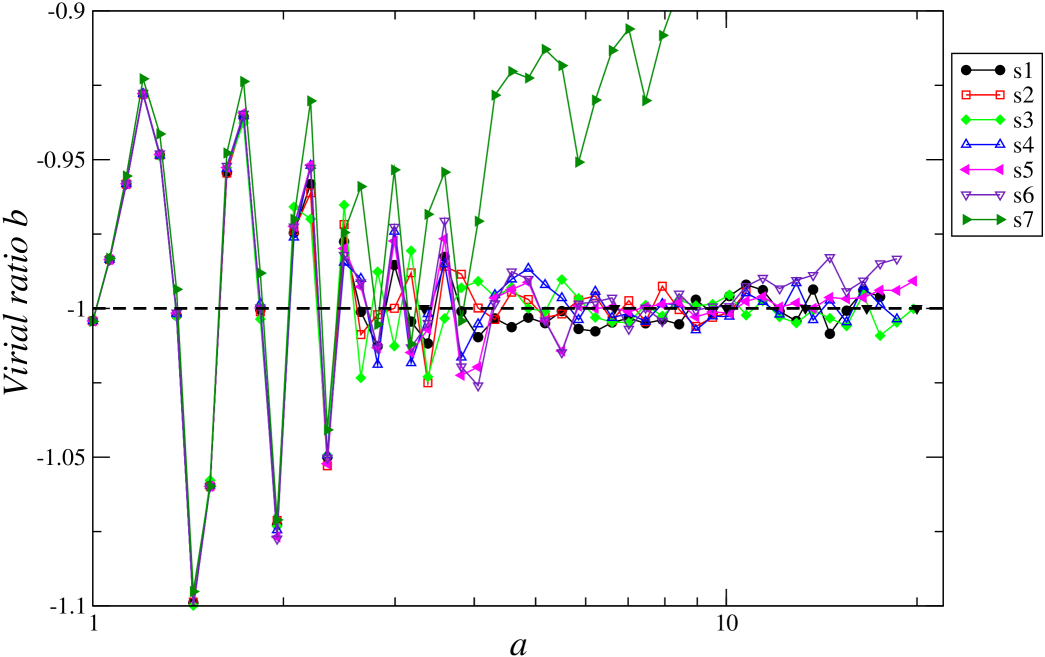
Figure 3: Evolution of the virial ratio $b$ (as defined in the text) up to scale factor $a=20$, for the different simulations in Table 1.

For all the simulations, except s7, the virial ratio evolves qualitatively as would be expected if the system evolves as in open boundary conditions: they show low amplitude coherent oscillations which decay gradually indicating virialisation (corresponding to $b=-1$). Further we have checked that there is good quantitative coherence between the amplitude and time scale of these oscillations, and those found in open boundary conditions (inset of Fig. 2): using Eq. (15) we see that the temporal range of the latter corresponds just to evolution up to $a\approx 2$ in the expanding case. We will consider below the exact degree of agreement between the density profiles obtained in the expanding simulations and the non-expanding case.

The fact that s7 behaves so differently — deviating clearly from a behavior like that in the other cases at $a\approx 5$ — can be attributed, as anticipated above, to the violation of the constraint (17): we have $\varepsilon/R_{s}\approx 0.04$ initially, which means that, if the structure does indeed remain fixed in physical coordinates, at $a\sim 5$ the effective mean-field force due to all particles is very different to its Newtonian value. For s6, on the other hand, with a smoothing about seven times smaller than in s7, we expect to have $\varepsilon/R_{s}\approx 0.1$ at $a=20$, still small enough so that the Newtonian value of the mean field potential is well approximated by the smoothed potential. In this latter case, however, even from $a\approx 10$ the virial ratio already appears in Figs.2 and 3 to show a slight tendency to increase at the larger values of $a$.

3.4.2 Potential energy

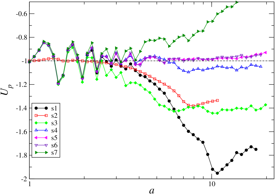
Figure 4: Evolution of the potential energy $U_{p}$ of the structure (in physical coordinates), for the indicated simulations in Table 1.

In Fig. 4 are shown the evolution of the physical potential energy $U_{p}$. If the structure, once virialized, remains stable in physical coordinates we should have $U_{p}=constant$. Further, of course, if the smoothing plays no role, this constant value should be the same in all the simulations. We observe that only the behavior observed for the simulations s5 and s6 appears to be consistent with stable clustering of the virialized structure, and even in these two cases a slight deviation is apparent at the end of simulated red-shift range, from $a\approx 18$. These plots thus indicate that at most in the corresponding narrow range of $\varepsilon$ can the behavior required in the desired continuum limit be reproduced by the $N$ body method.

3.4.3 Density profiles

Let us now examine whether this conclusion is borne out by further analysis of the evolved configurations. Shown in Fig. 5 are the measured density profiles at the indicated scale factors in each of the simulations. The results confirm strongly what can be anticipated from the analysis of the potential energy: the profiles agree increasingly poorly in time, with s7 and s1 clearly giving profiles completely different to those obtained in the other cases. s4, on the other hand, shows a much smaller discrepancy with the remaining two, s5 and s6. These latter two simulations agree very well with one another, except at the very last plot where a slight difference may be observed. We note that, compared to these cases, the simulations with a smaller $\varepsilon$ have a denser more concentrated core, while for s7, which has a larger value of $\varepsilon$, the opposite behavior is observed. This is very consistent with our comments above about this latter simulation: $\varepsilon$ is so large that mean field forces are very reduced compared to the exact Newtonian mean field, leading to a much less condensed structure.

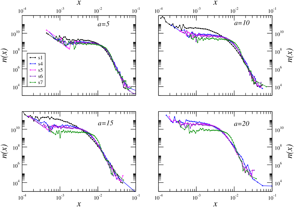
Figure 5: Density profiles in comoving coordinates as measured in the indicated simulations from Table 1, at the different indicated scale factors.

3.4.4 Rescaled density profiles

It can be seen qualitatively from the previous figures (which are plotted in comoving coordinates) that the comoving size of the structures does indeed decrease, with a corresponding increase in their density. To see whether the behavior is quantitatively in agreement with that associated with stable clustering, we show in Fig. 6 the evolution of the profile in physical coordinates for the simulations indicated, i.e., we plot in each case $n(r)=n(x)/a^{3}$ as a function of $r=ax$. In this representation stable clustering corresponds to an invariant profile. We also show in these plots the template for the profile of the collisionless equilibrium obtained from a simulation of the open non-expanding case, as described in Sect. 3.3. The insets in the plots show the results in each expanding simulation normalized to this profile.

The results confirm what has been anticipated above from the examination of the behaviour of $U_{p}$ and the comparison of density profiles, but also give additional constraints: s5 and s6 reproduce stable clustering considerably better than any of the other simulations, but s5 also clearly does better than s6, which shows a deviation between $a=15$ and $a=20$. Thus, of the full range of $\varepsilon$ considered, s5 is closest to optimal, while all others lead to quite measurable deviations from the continuum limit behaviour. We see very clearly in these plots again the marked qualitative difference between the cases of a smoothing which is too large and one which is too small. In the former case the structure obtained is very much less dense and more extended than it should be, while in the latter case it is very much more compact, with a density profile which steepens towards the centre. These differences, as we will discuss further in the final section below, clearly correspond to the very different effects at play in the two cases.

We note that the conclusions in the previous paragraph can be drawn even without the direct comparison with the non-expanding density profile: in other words, when stability is observed in a given expanding universe simulation, the (stable) profile obtained is always consistent with the correct one. The comparison with the non-expanding profile, shown in the inset of each figure gives a more quantitative measure of the deviation of the corresponding expanding universe simulation from the correct behavior. Note that these insets have been cut in all cases at $r=0.1$, since in all cases there are very significant deviations beyond this radius, which is reflected also clearly in clear deviations from stable clustering. Indeed we note that in all cases the very outer part of the profile extends very significantly further than in open boundary conditions. In most cases this corresponds to a very small fraction of the total mass, except in the case of s7 (with the largest smoothing) for which the characteristic size of the whole structure is, as we have noted, very much larger than it should be.

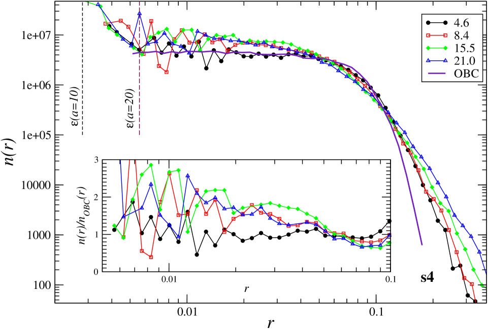
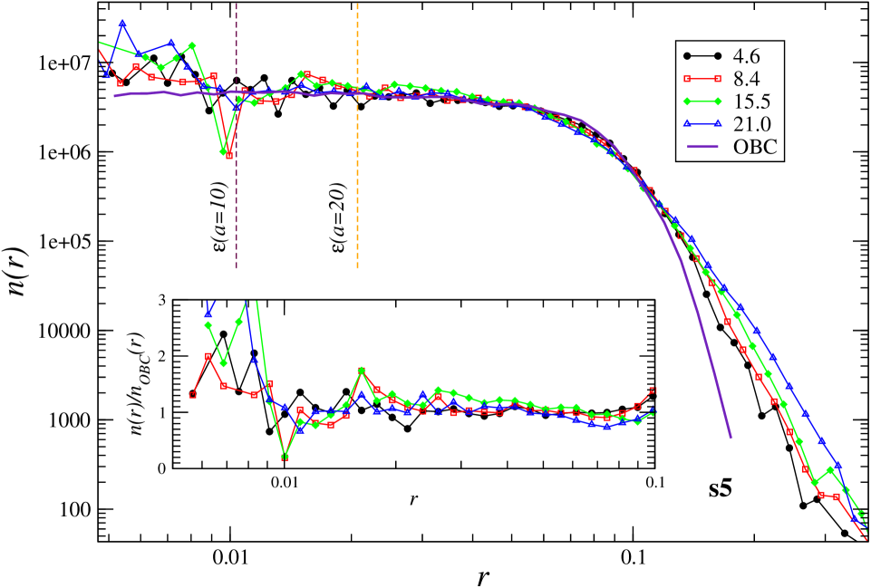
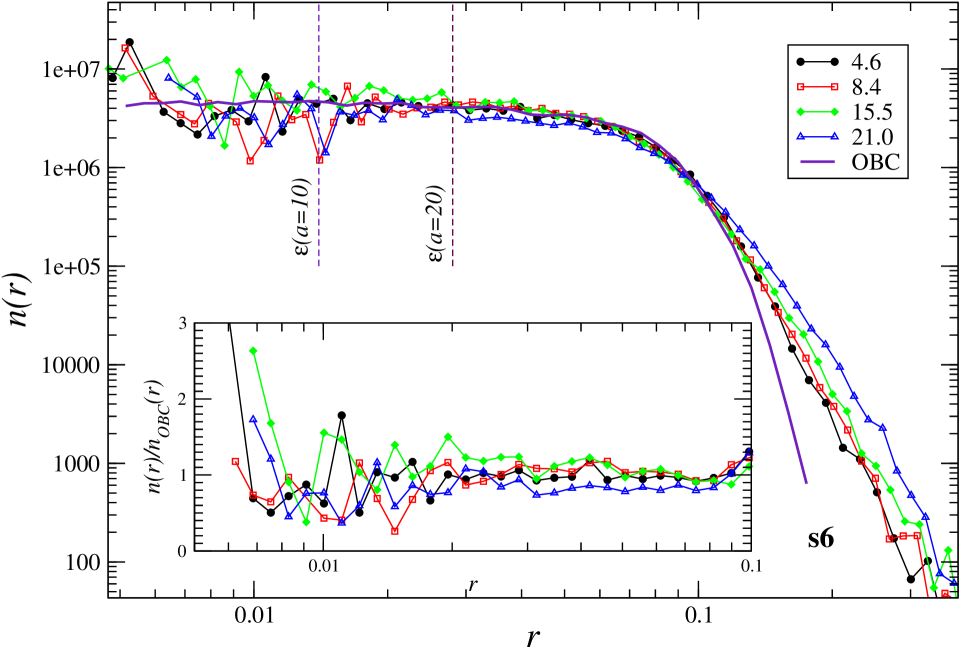
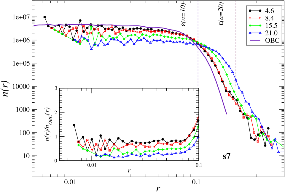
Figure 6: Density profiles in physical coordinates at the different indicated values of $a$. Each figure corresponds to the single indicated simulation. Also shown in each case is a smooth fit to the profile (labelled OBC) obtained in an open non-expanding simulation at $t=12\tau_{sc}$. In the inset plots of the profiles normalized by this latter profile are given.

3.5 Test for box size dependence

The simulations in the previous section are of fixed box size. The fact that they evolve differently is, by construction, due only to the different force smoothing. However when we compare the profiles obtained to the template in open boundary conditions (determined at very early times and taken to be representative of collisionless evolution), differences may also arise because of the periodic boundary conditions. As we have explained the differences with respect to the open system should be suppressed by powers of $R/L$ and thus vanish as the size of the system becomes small compared to the box size. By varying the box size we can test both whether finite size effects may be observed, and whether they are, as we have assumed, small for $R/L=0.1$

To do so we have run the set of simulations in Table 2. The simulation s5R0.1 is identical to the simulation s5 considered above, except that it has been run for a longer time, up to $a=33$ (rather than $a=20$). The other four simulations are for the same number of particles, $N=10^{4}$, and differ only in their initial size $R$. Because the overdensity $\delta$ represented by these initial conditions depends on $R$ [cf.Eq. (14)], the relation Eq. (15) between the physical time elapsed and the scale factor $a$ is modified. More precisely, in units of the characteristic time of the isolated structure $\tau_{sc}$, a given elapsed time $t-t_{0}$ corresponds to a fixed value of $R^{-3/2}\,(a^{3/2}-1)$. The scale factor $a=a_{\rm end}$ in Table 2, up to which the corresponding simulation has been run, has been chosen so that $R^{-3/2}\,(a_{\rm end}^{3/2}-1)$ is equal in all cases, i.e., all simulations are run up to the same time in units of $\tau_{sc}$.

The choice of $\varepsilon$ given in Table 2 have been made by scaling the value in s5 in proportion to $R$ (and the mean interparticle distance). As $\varepsilon$ is fixed in comoving coordinates, it evolves in physical coordinates in proportion to $a(t)$, and therefore as a function of $(t-t_{0})/\tau_{sc}$ in a manner which depends on the box size. Thus the dependence on box size in the evolution of these systems can arise not just from contributions to the gravitational force due to the periodic copies, but also through possible differences in the dynamics due to the differences in force smoothing in each case. Apart from such effects their evolution should be identical when analysed in physical units (of length and time).

Name	$\varepsilon$	$a_{\rm end}$
s5R0.3	1.1 $\times 10^{-3}$	100
s5R0.2	7.4 $\times 10^{-4}$	67
s5R0.1	3.7 $\times 10^{-4}$	33
s5R0.05	1.65 $\times 10^{-4}$	16.8
s5R0.025	8.25 $\times 10^{-5}$	8.6

Table 2: Parameter of simulations with $N=10^{4}$ particles for various different initial system size $R$ (in units of the side of the periodic box). The ratio $\varepsilon/R$ is the same as that in the simulation s5 in Table 1. The parameter $a_{\rm end}$ is defined in the text.

In Fig. 7 is shown the evolution of the potential energy $U_{p}$, normalized to the modulus of its initial value, for the five simulations, as a function of the appropriately normalised time determined by Eq. (15), and the evolution of the virial ratio in the inset. In Fig. 8 is shown the density profile in each of the five simulations, at the time in each case corresponding to $a=10$ in the simulation s5 (and s5R0.1).

Very strong dependence on the box size is manifest for the two largest systems (of which the initial diameter is equal to, respectively, $0.4$ and $0.6$ of the box size): both the energy of the virial equilibrium attained, and the density profiles, are very significantly different to those in the other cases. The smaller systems, on the other hand, show a clear convergence for these quantities (and which we have seen for the case s5R0.1 agree well with those obtained in the open case). The differences at late times in the deviations towards higher values of $U_{p}$, associated (as can be seen in the inset) with deviations from satisfaction of the virial condition, may clearly be attributed to the differences in the force smoothing noted above: a larger box size corresponds, at a given $(t-t_{0})/\tau_{sc}$, to a larger scale factor $a$, and therefore to a larger smoothing with respect to the size of the system. Indeed in the simulation s7 we saw (Fig. 4 ) that significant deviation in the behaviour of $U_{p}$ already at $a\sim 2-3$. The simulations here have $\epsilon/R_{s}$ initially exactly ten times smaller than in s7, and so would be expected to show deviations in the range $a\sim 20-30$ as is observed.

Thus for the quantities we have focussed on above the effects due to the finite box size in the system of the initial size we have considered appear indeed to be very small. We note, however, that considerable box size dependence is manifest even for the smaller boxes in other quantities. The amplitude of the oscillations during the initial relaxation to virial equilibrium are very significantly larger than in the smaller systems, for which the amplitude appears to converge approximately. This suggests that the corresponding modes of oscillation of the structure about the virial equilibrium are enhanced very significantly by the gravitational coupling to the periodic copies.

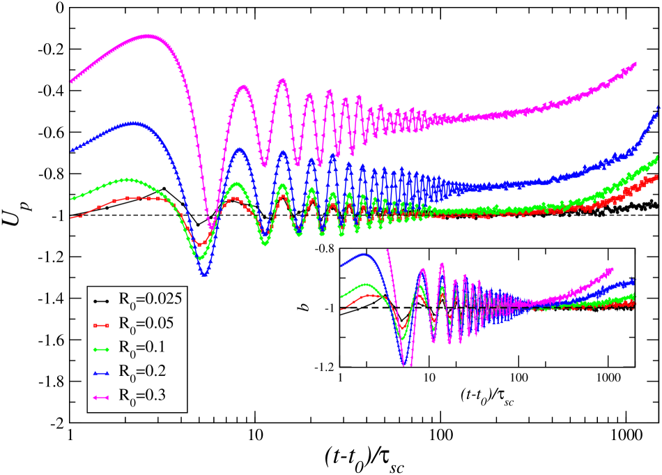
Figure 7: Evolution of the potential energy $U_{p}$ for the simulations in Table 2 with $N=10^{4}$, normalized to initial absolute value of $U_{p}$.

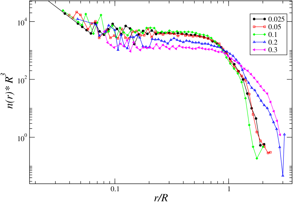
Figure 8: Density profiles for the simulations in Table 2 with $N=10^{4}$, at the normalized time corresponding to $a=10$ in s5R0.1

4 Comparison with the Layzer-Irvine test

One possible test of the accuracy of a cosmological code is the so-called Layzer-Irvine (LI) test, derived from the equation of the same name which describes the variation of total energy in an expanding universe (see, e.g., Peebles (1980)). Unlike energy conservation in non-expanding simulations, it is, however, a test which is rarely employed in practice by cosmological simulators as a control on their code, because it is not evident how to quantify the violation of the LI equation which may be tolerated. Given that the test discussed in this paper is an independent one on the correctness of cosmological codes in a specific regime, it can in principle be used to “calibrate” the LI test in this context. Likewise it is interesting to see whether it may be useful to employ both tests together.

In terms of the quantities defined above, the Layzer Irvine equation may be written (Peebles, 1980)

$$\frac{d}{dt}\left[a(K_{p}+U_{p})\right]=-\dot{a}K_{p}\,.$$ (21)

We thus define the quantity

$$A(a)=\frac{a(K_{p}+U_{p})+\int_{1}^{a}K_{p}da}{K_{p}(1)+U_{p}(1)}$$ (22)

which should be equal to unity .

In Fig. 9 is shown the evolution of $A(a)$ for the simulations s1 to s7. We observe immediately that the two simulations in which $A(a)$ remains close to unity are precisely those, s5 and s6, which have been singled out by our test above as reproducing best the required behaviour. On the contrary, all the other simulations which showed much greater deviation from stable clustering also show larger deviations from unity of $A(a)$. More precisely, in all cases where deviation of $A(a)$ from unity by more than a few percent is observed, the stable clustering test showed the results for the clustering in the system were completely incorrect and unphysical.

The correlation between the information we deduced from Fig. 4 and what we observe in Fig. 9 is very evident, and the reason for it very simple: the requirement that $U_{p}$ be constant is, when the virial condition $b=-1$ is satisfied, equivalent to the condition that both $K_{p}$, and therefore also the sum $U_{p}+K_{p}$ corresponding to the energy in physical coordinates, is constant. In this case, as can be seen from Eqs. (21) and (22), the LI test is also satisfied. Thus it is clear that the very strong deviations from stable clustering observed for the simulations s1 to s4 stem from a poor integration of the equations of motion, with very significant violation of energy conservation. As discussed in Sect. 3.2, such numerical difficulties are expected to arise due to the precision requirements of integrating accurately the hard two body collisions present when $\varepsilon$ becomes very small. We note that our results are very consistent with those of Knebe et al. (2000) who have studied in detail the effects of such poorly integrated hard collisions: they lead to an artificial injection of energy into the system, increasing its size as some particles are sent into spurious higher energy orbits. We observe here indeed quite distinctly these effects both in the behaviour of the energy (which increases) and the profiles which stretch out further than they should (compared to stable clustering).

For the very small $\varepsilon$ considerably greater precision than that employed (see Appendix A) would be required to attain numerical convergence. We note that our results do suggest that, at given numerical precision, a lower bound on $\varepsilon$ may be expressed in a simple form like Eqs. (18)-(20), i.e., that the minimal $\varepsilon$ required scales linearly the size of the structure $R_{s}$ : in Fig. 4 each of the simulations s1 to s3, which have the same maximum time step, show an approximate plateau in $U_{p}$, starting from a scale factor $a$ which increases roughly in proportion to $1/\varepsilon$. Given that we observe in these simulations that $R_{s}\sim 1/a$, this behaviour of $U_{p}$, indicating energy conservation, therefore sets in approximately at a fixed value of $\varepsilon/R_{s}$, in line with bounds of the form of Eqs. (18)-(20). A study of simulations with different $N$ would be required to establish which (if any) of the proposed scalings is the correct one

We underline that the LI test for an expanding simulation is, just as the test for the constancy of $U_{p}$, a weaker test than the test for the stability of clustering: the latter tests for the collisionless nature of the evolution, which is a different (and stronger) requirement than energy conservation. In practice, however, the breakdown of energy conservation is often due to the difficulty of integrating numerically with sufficient accuracy the collisional dynamics (specifically, hard two body collisions), and therefore the breakdown of the collisionless approximation is associated with the violation of energy conservation. Such an association can always be “undone” , in principle, by increasing sufficiently the accuracy of the numerical integration. In practice, however, it is very difficult to disentangle the two effects, and indeed studies up to now of two body collisionality in cosmological simulations (e.g. Knebe et al. (2000); Power et al. (2003); Binney & Knebe (2002)) have not done so.

In conclusion we find that the LI test is a very useful and relevant one in the context of the present test of cosmological simulations. Quite simply deviations of the dimensionless parameter $A$ defined above by more than a few percent appear always to be indicative of a grossly incorrect evolution. The crucial difference with respect to its use for a full cosmological simulation, which, as mentioned, has been found to be problematic, arises from the difference in initial condition: for the very cold and almost perfectly uniform initial conditions of cosmological simulations the denominator in $A$ approaches zero, which makes it difficult to calibrate the test.

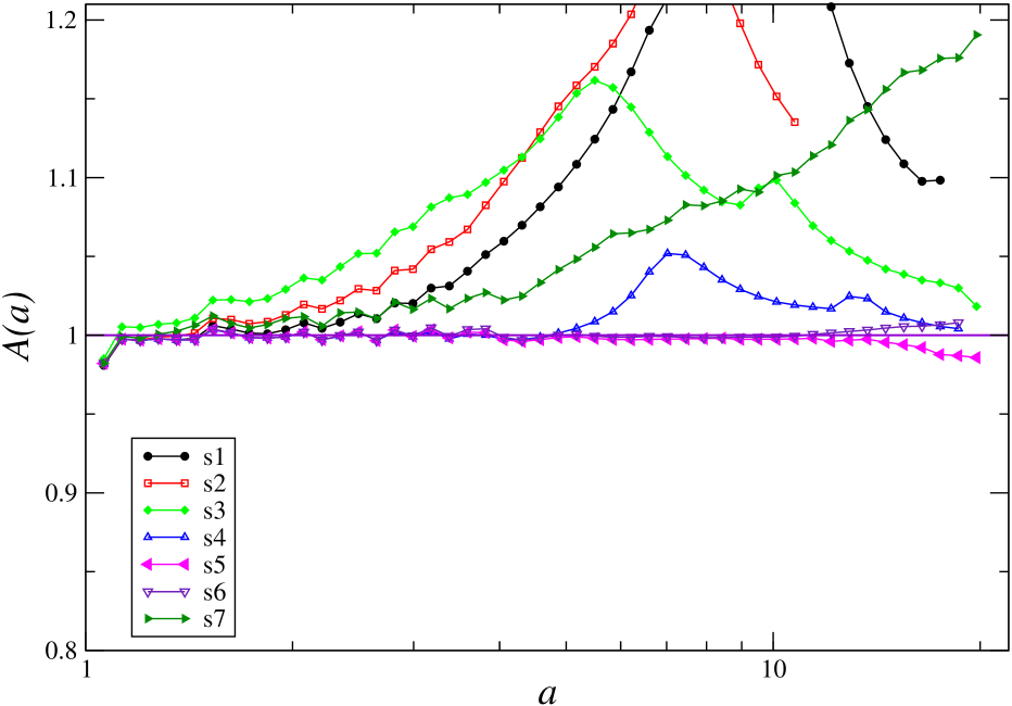
Figure 9: Layzer Irvine test for the simulations in Table 1. See text for the definition of $A(a)$.

5 Nature of discreteness effects and parametric scalings

Our results above establish that the tests considered can clearly detect and measure discreteness effects in $N$-body simulations, i.e., deviations of the results of such simulations from the desired continuum limit. We discuss now briefly what conclusions may be drawn about the nature of these discreteness effects. More specifically we discuss what we can conclude about the parametric dependences of these effects.

Discreteness effects here can be divided into two categories as follows:

• “numerical discreteness effects” arising arise from limitations on precision in the integration of the $N$-body system with a given smoothed two-body potential, and

• “physical discreteness effects” arising from the use of a finite particle density, finite force smoothing and a finite periodic box.

The former are related to the choice of the numerical parameters controlling accuracy of the force calculation and time stepping in the code, while the latter are related to the number of particles $N$, the size of the force smoothing $\varepsilon$ and the size of the box $L$ . The two kinds of effects are in practice interrelated since the numerical precision required will depend typically on the values of the “physical” discreteness parameters. However, in order to understand the effects at play in cosmological simulation, it is useful to separate them in this way. One can then consider, on the one hand, the issue of numerical convergence at fixed values of $N$, $\varepsilon$ and $L$, and, on the other hand, the scalings with $N$, $\varepsilon$ and $L$, of the deviations from the desired physical behaviour, assuming “perfect” numerical convergence. It is the latter we consider here. Our results in Sect. 3.5 showed up clearly the presence of effects related to the box size $L$, which, in line with expectations, decrease strongly as $L$ increases compared to the size of the simulated structure. We do not pursue further tests here to establish exactly the associated scalings, but instead focus on the other two parameters.

Our results show clearly, as anticipated, that for larger values of the smoothing, deviation from the collisionless self-gravitating limit arises predominantly from the associated loss of spatial resolution. This was most easily “diagnosed” by the behaviour of the virial ratio, which deviated clearly away from $b=-1$ towards less negative values. As discussed in Sect. 3.5 the behaviours observed are very consistent with the simple bound Eq. (17), with significant deviations becoming easily visible (in potential energy and profiles) roughly when $(\varepsilon/R_{s})\sim 0.1$. Using the fact that $R_{s}\propto 1/a$, we deduce that the scale factor at which we see the effects of the finite resolution start to significantly modify the structure is

$$a_{res}\sim 10^{-1}\frac{R}{\varepsilon}$$ (23)

where $R$ is the size of the structure at $a=1$ (and the result is valid for the case we consider where $\varepsilon$ remains fixed in comoving coordinates).

The very large deviations from stable clustering we have observed in our simulations with very small $\varepsilon$ are, as we have discussed, apparently due to poor integration of hard two body collisions. This problem is clearly diagnosed very well using analysis of the $U_{p}$, or even more clearly using the LI test. As mentioned, such effects have been diagnosed and discussed in some detail notably in Knebe et al. (2000).

In principle, as we have discussed, two body collisionality, when integrated accurately, can also contribute to the deviations from stable clustering we observe. Indeed in our simulations s5 and s6, which satisfy quite precisely the LI test, we see clear deviations which are similar qualitatively to those observed in the case of poorly integrated collisions: tails in the density profiles which become more extended in time and a hint of steepening of the inner density profile. It is straightforward in our case to estimate the time scale for such two body effects using the well known results for the case of an open virialized system in a non-expanding space. In this case numerical studies (see e.g. Farouki & Salpeter (1982, 1994); Theis (1998); Theis & Spurzem (1999); Diemand et al. (2004); Gabrielli et al. (2010)) have shown that the time scales for evolution of collisionless equilibria is very consistent with the those estimated analytically (originally by Chandrasekhar, see Chandrasekhar (1943)) for two body collisions, given by

$$\tau_{2body}\approx\kappa N\tau_{c}$$ (24)

where $\tau_{c}$ is a characteristic crossing time for the structure, and $\kappa$ is a numerical factor incorporating the “Coulomb logarithm” . Modulo box size effects, which we have seen are small, the only difference between these open systems and the one we are studying should arise from the difference in the smoothing, which in our cosmological code simulations is fixed in comoving coordinates and therefore varies in time (increases) in physical coordinates. The two body relaxation time is, however, only logarithmically sensitive to the lower cut-off in the two body interaction, and temporal variation of the smoothing $\varepsilon$ will lead therefore to modification of the numerical prefactor $\kappa$ in the calculation, with at most very weak dependence on $N$. Using Eq. (15) with Eq. (24) we thus estimate that two body relaxation will start to cause deviations in our numerically well converged test simulations (i.e. s5 and s6 above) when

$$a_{2body}\sim\left[\frac{\kappa(\varepsilon)}{\sqrt{\delta}}\,N\right]^{2/3}$$ (25)

where we have taken $\tau_{c}\sim\tau_{sc}$.

Values of $\kappa$ of order those measured in open simulations (with smoothing fixed in physical coordinates), typically a little smaller than unity, thus give an estimate for $a_{2body}$ quite consistent with the hypothesis that two body collisionality should account for the observed deviations from stable clustering in the simulations in which the energy is conserved well. We note that these results also appear to be very consistent with studies such as Power et al. (2003); Binney & Knebe (2002) which have detected such effects in cosmological simulations. Clearly however a full study of the $N$-dependence of the results of our test, which we do not undertake here, would be required to establish whether the scaling Eq. (25) is indeed observed. It would be instructive to couple such a study also to one including analysis with other indicators of collisionality (e.g. measures of diffusion in velocity space like those employed in Diemand et al. (2004), or using two mass species as in Binney & Knebe (2002)).

An important practical question in numerical simulation is whether there is an optimal value of force smoothing in cosmological N body simulations. The question may be posed either with respect to some set of numerical constraints (quantified e.g. in terms of bounds on the numerical parameters controlling accuracy of integration), or in abstraction from such limitations. The relations Eq. (25) and Eq. (23) can be clearly combined, in principle, to provide a prescription for an optimal value of the latter kind: although we have not determined explicitly, it is clear that $\kappa(\varepsilon)$ is a monotonically (a priori logarithmically) increasing function of $\varepsilon$, while the coefficient in Eq. (23) is monotonically decreasing. Thus by varying $\varepsilon$ at fixed $N$ an optimal value can be found which maximizes the scale factor at which discreteness effects modify the evolution. A much more extensive study, notably of $N$ dependence, would clearly be necessary to determine the scaling with $N$ of such an optimum. It would be interesting to determine, in particular, whether it turns out to be that derived by Merritt (1996); Dehnen (2001) from simple considerations of the optimization of the representation of the continuum (mean-field, Newtonian) forces. It would evidently be interesting also to compare with optimization criteria derived in various numerical convergence studies in the literature (e.g. Diemand et al. (2004); Power et al. (2003)).

6 Practical guide to use of the test

The numerical study we have reported establishes that the test considered can provide non-trivial constraints on the accuracy of cosmological simulations. To facilitate the exploitation of the test in practice by cosmological simulators we now summarize in a recipe form how it could be implemented. The results of such tests will, as we discuss, inevitably depend strongly on the details of the particular simulations (cosmological model, time and length scales probed, quantities of interest and desired level of precision etc). We therefore do not attempt to summarize the information which can be obtained from the test in some simple set of rules. Instead we propose to simulators an instrument they can use to assess themselves the reliability of the results of their codes.

Let us suppose a simulator intends to run a (dissipationless) cosmological simulation, which has $N_{\rm 0}$ particles of mass $m$ in a box of side $L_{\rm 0}$. An initial perturbation spectrum $P(k)$ is given at the starting red-shift $z_{i}$, and a cosmological model specifying the scale-factor (e.g. $\Lambda$ CDM). Based on criteria at his disposal, he chooses a set of numerical parameters (time step and force accuracy criteria, smoothing $\varepsilon$). The test we have considered for the accuracy of simulation of halos containing $N$ particles (and of mass $M=mN$) can be generalized as follows:

• Consider a simulation identical for all numerical parameters to the full simulation, except for the box size, which is rescaled so that

  $$L=L_{0}\left(\frac{N}{N_{0}}\right)^{1/3}$$ (26)

  This condition means that the mean matter density of the universe is equal to that in the full simulation, and therefore, in particular, the ratio $\varepsilon/\ell$ has the same value as in the full simulation.

• Distribute the $N$ particles in a spherical region of radius $R=L(3\rho_{0}/4\pi\rho_{v})^{1/3}$ where $\rho_{v}$ is the initial density of the halo. For $\rho_{v}\approx 200\rho_{0}$ this corresponds to $R\approx 0.1$ (as in our simulations s1-s7 above).

• Assign velocities with some simple velocity distribution (e.g. uniform or gaussian) and normalize them so that the initial virial ratio is unity.

• Run the cosmological code (with the chosen numerical parameters) starting from $z_{v}(M)$, the (estimated) maximum redshift for virialization of a halo of mass $M$ in the model studied.

• Check that the potential energy $U_{p}$ and virial ratio $b$ display the expected physical behaviour (low amplitude decaying oscillations about a constant value). Systematic deviation of the virial ratio from $b=-1$ towards less negative values indicates that the upper resolution on smoothing is violated. Plot also the parameter $A(a)$ for the LI test. If deviations from unity are at the level of more than a few percent, the parameter choices are inappropriate to simulate over the corresponding time-scale.

• To obtain more precise limits on the precision of halo profiles (in the cases where the previous tests are reasonably well satisfied) apply first the test for stability of clustering. Further quantitative limits can be obtained by comparison with the equilibrium profile obtained from a high-resolution simulation of the same initial conditions in open boundary conditions.

Our simulations s1-s7 reported above test the case $N=10^{4}$ for a range of values of $\varepsilon$ (and other numerical parameters) up to red-shift of about twenty. Following the prescription above we would exclude all but s5 and s6 using the analysis of the energies and LI test beyond a red-shift of a few (cf. Fig. 4 and Fig. 9). The conclusion of our further analysis (step 6) above was that significant departures from stable clustering (and from the equilibrium template) were observable, increasing as a function of redshift. Beyond a redshift of order ten, we could conclude, for example, that $50\%$ precision on profiles of halos over two decades in scale is not attainable with $N=10^{4}$. To determine how many particles (and what numerical parameters) would lead to such a level of precision could be determined by performing the test for larger $N$.

Several variants of the test as described above could provide further or more precise constraints:

• Different initial conditions could be used in steps 2 and 3. In particular rather than a structure close to, but not at, virial equilibrium, one could take instead a structure which is already at equilibrium. Such an initial condition could be prepared numerically, or set up directly using the Eddington formula (see, e.g., Muldrew et al. (2011); Kazantzidis et al. (2004)). It would be interesting notably to study equilibrium halos with profiles like those typically measured in simulations (e.g. NFW halos). Alternatively initial conditions could be obtained directly from the full cosmological simulation, by extracting typical halos at about the time they virialize. Techniques to do this have been developed in the context of convergence studies in which individual halos are identified and resimulated at higher resolution(see, e.g. Power et al. (2003) and references therein).

• To separate out possible effects arising from the box size, the test could be repeated in boxes of different sizes, and specifically in a box of side $L_{0}$. These are important in particular when comparison with a simulation in open boundary conditions is made. As the change in the box size leads to a change in the mean density (by a factor of $N/N_{0}$ for the case of a box of size $L_{0}$), this must be accounted for in applying the test. As discussed in Sect. 3.5, in an EdS cosmology this can done, modulo effects due to the force smoothing, by a simple rescaling of the time. If the role of smoothing is the focus of the test, and/or the cosmology employed is non-scale free (e.g. $\Lambda$CDM,) the code would need to be modified “by hand” to impose the evolution of the scale factor corresponding to the cosmological simulation.

• Another variant of the test would be, using further the framework of the spherical collapse model for halo formation, to start from the time of turn-around. At this time the spherical overdensity is already sufficiently large ($\sim 5-6$) that one should be able to consider the system to a good approximation as isolated. The initial condition would thus be taken as a uniform or quasi-uniform sphere with physical velocities equal to zero. Given that the scale $R$ in step 1 would be comparable to the box size, it would be appropriate also to study simulations in a larger box as discussed in the previous paragraph.

7 Conclusions and discussion

The central point of this paper is the introduction of a simple test on the reliability of cosmological $N$-body simulations in the non-linear regime. We have shown with a very simple implementation of the test that it can constrain strongly the choice of the unphysical parameters introduced by the $N$-body method, given desired precision criteria on the properties of virialized structures. More specifically we have illustrated that the test can determine a window for an appropriate force smoothing $\varepsilon$ for simulations with a given time stepping accuracy, and any given $N$ in a virialized structure. At larger $\varepsilon$ the loss of resolution was clearly seen to be the dominant effect, while at small $\varepsilon$ the effects of two body collisionality become the primary cause of deviation. In contrast to most other methods explored previously in the literature these effects are detected and quantified by comparing the evolution of the test simulation with an exact behaviour, rather than by a comparison between different codes.

We have not attempted here, and indeed it is not our goal, to try to use the test to derive some set of simple short-hand rules that could be used to, say, choose $\varepsilon$ in a given cosmological simulation (or compared with other prescriptions which have been given in the literature). Rather it is the simulator who should apply the test to derive what his constraints are, with respect to his own precision requirements. Nevertheless it is interesting to comment a little more on what our specific test, of simulations with fixed comoving softening, indicates. Smoothing in simulations with fixed comoving softening are characterised by the sole parameter $\varepsilon/\ell$. We can compare the smoothings we have considered (Table 1) to typical values employed in large volume cosmological simulations: the smoothing in s5, s6 and s7 correspond, respectively, to $\varepsilon/\ell\approx 1/125,1/100,1/12$, while e.g., Springel et al. (2005) uses $\varepsilon/\ell\approx 1/50$, and Smith et al. (2003) $\varepsilon/\ell\approx 1/16$. From the results discussed above it is clear that application of the test for these specific values can give very strong indications of the reliability and/or precision of the properties of halos in such simulations. Indeed we note that, using Eq. (14), our approximate derived constraint Eq. (23) for the red-shift range over which a structure of $N$ particles may be resolved, can be rewritten as

$$a_{res}\sim 10^{-2}\frac{\ell}{\varepsilon}\,N^{1/3}\,.$$ (27)

Thus, for example, at $\frac{\ell}{\varepsilon}\sim 10^{-2}$ resolution constraints become relevant for all objects of less than $N\sim 10^{3}$ formed at or before a redshift of ten.

Comparing this with Eq. (25), in which the factor $\kappa(\varepsilon)$ has a priori very weak (logarithmic) dependence on $N$, leads to the conclusion that, for given $\varepsilon/\ell$, two body collisionality will be the dominant discreteness effect at small $N$, while for larger $N$ it is the resolution limit associated with $\varepsilon$ which is the relevant one. Thus, for an $\varepsilon/\ell$ which remains fixed in comoving coordinates, there is an inevitable trade-off between resolution and the introduction of spurious discreteness effects. We have considered solely simulations with fixed comoving softening, but the test can be applied without modification (as described in detail in that last section) to any other kind of code. Indeed it could provide very useful constraints on optimal smoothing strategies in codes with an adaptative smoothing, which indeed aim to optimize spatial resolution while keeping two body collisionality under control (see e.g. Knebe et al. (2000)).

We finally remark that while the test discussed here can, as we have shown, provide constraints on the parameters which must be respected in order to reproduce the desired continuum limit, it does not show that satisfaction of these constraints guarantee the same property, i.e., the test provides necessary, but not sufficient, conditions to guarantee the correctness of the numerical results. Firstly the test only constrains the choice of parameters in the strongly non-linear regime. This means, notably, that it cannot say anything about the appropriateness of the use of an $\varepsilon<\ell$, which has been shown to introduce discreteness effects in the early time evolution, and which may or may not distort the subsequent evolution (Splinter et al. (1998); Joyce et al. (2008); Romeo et al. (2008); Knebe et al. (2000)). Nor can it, as noted, provide constraints on the choice of the starting redshift of simulations (Joyce et al. (2008); Knebe et al. (2009)). Further, even in the non-linear regime, it is clear that considerable caution should be adapted in supposing the constraints derived from this test guarantee a faithful representation of the collisionless evolution: it shows that halos with less than some number of particles will necessarily suffer from effects of discreteness which modify strongly their density profiles: as we have seen in our study, the use of a smoothing which is slightly too small leads at the end of the simulation to a completely incorrect profile. Further the characteristic physical scale of this modification is the size of the structure, which has no direct relation to the smoothing scale $\varepsilon$. In the case of an inappropriately large $\varepsilon$ (simulation s7 above) we saw that a halo can even be very considerably larger than it should be. How the presence of such spurious clustering modifies the evolution of the whole system is very unclear. Indeed given that clustering in currently favored cosmological models is hierarchical in nature, the possibility that such error may feed through different scales is a major concern.

We thank François Sicard for useful discussions, and the two anonymous referees for many invaluable criticisms and suggestions.

Appendix A Further details on simulations

Besides the choice of $\varepsilon$ on which we have focussed above, simulation with GADGET requires one to fix several other numerical parameters. In our choices we have followed the guidelines given by the GADGET user’s guide, and also performed several tests indicate that our results appear to be reasonably stable with respect to these choices. Specifically we have considered:

• ErrTolIntAccuracy, a dimensionless parameter which controls the accuracy of the time-step criterion. The value suggested by the GADGET user’s guide is 0.025, and we have done numerical tests in various cases reducing it by a factor ten without any detectable difference in the results reported here.

• MaxSizeTimestep, which specifies the maximum allowed time-step for cosmological simulations as a fraction of the current Hubble time. According to the GADGET user’s guide a value of 0.025 is usually accurate enough for most cosmological runs. We have found our results to be stable in tests using considerably smaller values, down to as small as $10^{-5}$ in some cases.

• ErrTolTheta is the accuracy criterion (the opening angle $\theta$) of the tree algorithm if the standard Barnes & Hut (BH) opening criterion is used. The suggested value is 0.7 and we have considered values down to 0.1, again finding stable results in the tested cases.

We have also performed some tests comparing different realizations of the initial conditions in various cases, again with stable results.

We emphasize that despite these numerous tests, we have come to the conclusion through our analysis using the test studied in the paper that the four simulations with smaller $\varepsilon$ are in fact not numerically converged, and are characterized by very significant violations of energy conservation due to poorly integrated two body collisions. Thus sufficient further extrapolation of the numerical parameters beyond what we have considered must lead to very different results in these cases.

For completeness we give in Table 3 I the values of the numerical parameters used in the simulations reported in the body of the article. For the non-expanding simulation in open boundary conditions we have used (see also Sylos Labini (2012) for further details), a force softening $\varepsilon=0.007R$. This means that $\varepsilon$ is very much smaller at all times than the size of the structure. In addition we have chosen $\eta=0.01$, and have used the new GADGET cell opening criterion with a high force accuracy of $\alpha_{F}=0.001$. Energy is conserved to within less than $10^{-3}$ up to $12\tau_{sc}$. In Joyce et al. (2009) extensive tests of the dependence on $\varepsilon$ were performed, for the much more constraining case of evolution from the same initial condition but with initial velocities set to zero. These tests lead to the conclusion that no sensible dependence is observed up to this time (notably in the density profile) unless the ratio $\varepsilon/R_{s}$ becomes large.

Simulation	ETIA	MaxTimeStep	ErrTolTheta
s1	0.025	0.01	0.7
s2	0.0025	0.01	0.7
s3	0.0025	0.01	0.7
s4	0.025	0.0001	0.7
s5	0.025	0.0001	0.7
s6	0.025	0.00001	0.1
s7	0.025	0.0001	0.7
s1N5e4	0.025	0.01	0.7
s1N1e5	0.025	0.01	0.7
s5N1e3	0.025	0.0001	0.7
s6N1e3	0.025	0.00001	0.1

Table 3: Values of the three numerical parameters (ErrTolIntAccuracy, MaxTimeStep and ErrTolTheta) adopted in each of the simulations reported in the text.

References

- Bagla (2005) Bagla J., 2005, Curr. Sci., 88, 10883
- Binney & Knebe (2002) Binney J., Knebe A., 2002, Mon. Not. R. Astron. Soc., 333, 378
- Chandrasekhar (1943) Chandrasekhar S., 1943, Rev. Mod. Phys., 15, 1
- Dehnen (2001) Dehnen W., 2001, Mon. Not. R. Astron. Soc., 324, 273
- Diemand et al. (2004) Diemand J., Moore B., Stadel J., Kazantzidis S., 2004, Mon. Not. R. Astron. Soc., p. 977
- Efstathiou et al. (1988) Efstathiou G., Frenk C. S., White S. D. M., Davis M., 1988, Mon. Not. R. Astron. Soc., 235, 715
- Farouki & Salpeter (1982) Farouki R. T., Salpeter E. E., 1982, Astrophys. J., 253, 512
- Farouki & Salpeter (1994) Farouki R. T., Salpeter E. E., 1994, Astrophys. J. Lett, 427, 676
- Gabrielli et al. (2006) Gabrielli A., Baertschiger T., Joyce M., Marcos B., Sylos Labini F., 2006, Phys. Rev., E74, 021110
- Gabrielli et al. (2010) Gabrielli A., Joyce M., Marcos B., 2010, Phys. Rev. Lett., 105, 210602
- Gabrielli et al. (2004) Gabrielli A., Sylos Labini F., Joyce M., Pietronero L., 2004, Statistical Physics for Cosmic Structures. Springer
- Heggie & Hut (2003) Heggie D., Hut P., 2003, The Gravitational Million-Body Problem: A Multidisciplinary Approach to Star Cluster Dynamics. Cambridge
- Heitmann et al. (2005) Heitmann K., Ricker P. M., Warren M. S., Habib S., 2005, Astrophy. J. Supp, 160, 28
- Joyce et al. (2008) Joyce M., Marcos B., Baertschiger T., 2008, Mon. Not. R. Astron. Soc.
- Joyce et al. (2009) Joyce M., Marcos B., Sylos Labini F., 2009, Mon. Not. R. Astron. Soc., 397, 775
- Kazantzidis et al. (2004) Kazantzidis S., Magorrian J., Moore B., 2004, Astrophys. J., 601, 37
- Knebe et al. (2000) Knebe A., Kravtsov A., Gottlöber S., Klypin A., 2000, Mon. Not. Roy. Astron. Soc., 317, 630
- Knebe et al. (2009) Knebe A., Wagner C., Knollmann S., Diekershoff T., Krause F., 2009, Astrophys. J., 698, 266
- Kravtsov et al. (1997) Kravtsov A. V., Klypin A. A., Khokhlov A. M., 1997, Astrophys. J. Supp., 111, 73
- Merritt (1996) Merritt D., 1996, Astron. Jour., 111, 2462
- Muldrew et al. (2011) Muldrew S. I., Pearce F. R., Power C., 2011, Mon. Not. R. Astron. Soc., 410, 2617
- Peebles (1980) Peebles P. J. E., 1980, The Large-Scale Structure of the Universe. Princeton University Press
- Power et al. (2003) Power C., Navarro J. F., Jenkins A., Frenk C. S., White S. D. M., Springel V., Stadel J., Quinn T., 2003, Mon. Not. R. Astron. Soc., 338, 14
- Romeo et al. (2008) Romeo A. B., Agertz O., Moore B., Stadel J., 2008, Astrophys. J., 686, 1
- Smith et al. (2003) Smith R. E., Peacock J. A., Jenkins A., White S. D. M., Frenk C. S., Pearce F. R., Thomas P. A., Efstathiou G., Couchman H. M. P., 2003, Mon. Not. R. Astron. Soc., 341, 1311
- Splinter et al. (1998) Splinter R. J., Melott A. L., Shandarin S. F., Suto Y., 1998, Astrophys. J., 497, 38
- Springel et al. (2005) Springel V., et al., 2005, Nature, 435, 629
- Springel et al. (2001) Springel V., Yoshida N., White S. D. M., 2001, New. Astron., 6, 79
- Sylos Labini (2012) Sylos Labini F., 2012, Mon. Not. R. Astron. Soc., 423, 1610
- Teyssier (2002) Teyssier R., 2002, Astron. Astrophys., 385, 337
- Theis (1998) Theis C., 1998, Astron. Astrophys., 330, 1180
- Theis & Spurzem (1999) Theis C., Spurzem R., 1999, Astron. Astrophys., 341, 361
- Worrakitpoonpon (2011) Worrakitpoonpon T., , 2011, PhD. Thesis, Université Pierre et Marie Curie