Kullback–Leibler upper confidence bounds for optimal sequential allocation

Abstract

We consider optimal sequential allocation in the context of the so-called stochastic multi-armed bandit model. We describe a generic index policy, in the sense of Gittins [J. R. Stat. Soc. Ser. B Stat. Methodol. 41 (1979) 148–177], based on upper confidence bounds of the arm payoffs computed using the Kullback–Leibler divergence. We consider two classes of distributions for which instances of this general idea are analyzed: the kl-UCB algorithm is designed for one-parameter exponential families and the empirical KL-UCB algorithm for bounded and finitely supported distributions. Our main contribution is a unified finite-time analysis of the regret of these algorithms that asymptotically matches the lower bounds of Lai and Robbins [Adv. in Appl. Math. 6 (1985) 4–22] and Burnetas and Katehakis [Adv. in Appl. Math. 17 (1996) 122–142], respectively. We also investigate the behavior of these algorithms when used with general bounded rewards, showing in particular that they provide significant improvements over the state-of-the-art.

, , , and

t1Supported by the French National Research Agency (ANR) under Grant EXPLO/RA (“Exploration–exploitation for efficient resource allocation”), the PASCAL2 Network of Excellence under EC Grant 506778 and the ECs Seventh Framework Programme (FP7/2007–2013) under Grant agreement no. 270327.

1 Introduction

This paper is about optimal sequential allocation in unknown random environments. More precisely, we consider the setting known under the conventional, if not very explicit, name of (stochastic) multi-armed bandit, in reference to the 19th century gambling game. In the multi-armed bandit model, the emphasis is put on focusing as quickly as possible on the best available option(s) rather than on estimating precisely the efficiency of each option. These options are referred to as arms, and each of them is associated with a distribution; arms are indexed by $a$ and associated distributions are denoted by $\nu_{a}$.

The archetypal example occurs in clinical trials where the options (or arms) correspond to available treatments whose efficiencies are unknown a priori, and patients arrive sequentially; the action consists of prescribing a particular treatment to the patient, and the observation corresponds (e.g.) to the success or failure of the treatment. The goal is clearly here to achieve as many successes as possible. A strategy for doing so is said to be anytime if it does not require to know in advance the number of patients that will participate to the experiment. Although the term multi-armed bandit was probably coined in the late 1960s [Gittins (1979)], the origin of the problem can be traced back to fundamental questions about optimal stopping policies in the context of clinical trials [see Thompson (1933, 1935)] raised since the 1930s; see also Wald (1945), Robbins (1952).

In his celebrated work, Gittins (1979) considered the Bayesian-optimal solution to the discounted infinite-horizon multi-armed bandit problem. Gittins first showed that the Bayesian optimal policy could be determined by dynamic programming in an extended Markov decision process. The second key element is the fact that the optimal policy search can be factored into a set of simpler computations to determine indices that fully characterize each arm given the current history of the game [Gittins (1979), Whittle (1980), Weber (1992)]. The optimal policy is then an index policy in the sense that at each time round, the (or an) arm with highest index is selected. Hence, index policies only differ in the way the indices are computed.

From a practical perspective, however, the use of Gittins indices is limited to specific arm distributions and is computationally challenging [Gittins, Glazebrook and Weber (2011)]. In the 1980s, pioneering works by Lai and Robbins (1985), Chang and Lai (1987), Burnetas and Katehakis (1996, 1997, 2003) suggested that Gittins indices can be approximated by quantities that can be interpreted as upper bounds of confidence intervals. Agrawal (1995) formally introduced and provided an asymptotic analysis for generic classes of index policies termed UCB (for Upper Confidence Bounds). For general bounded reward distributions, Auer, Cesa-Bianchi and Fischer (2002) provided a finite time analysis for a particular variant of UCB based on Hoeffding’s inequality; see also Bubeck and Cesa-Bianchi (2012) for a recent survey of bandit models and variants.

There are, however, significant differences between the algorithms and results of Gittins (1979) and Auer, Cesa-Bianchi and Fischer (2002). First, UCB is an anytime algorithm that does not rely on the use of a discount factor or even on the knowledge of the horizon of the problem. More significantly, the Bayesian perspective is absent, and UCB is analyzed in terms of its frequentist (distribution-dependent or distribution-free) performance, by exhibiting finite-time, nonasymptotic bounds on its expected regret. The expected regret of an algorithm—a quantity to be formally defined in Section 2—corresponds to the difference, in expectation, between the rewards that would have been gained by only pulling a best arm and the rewards actually gained.

UCB is a very robust algorithm that is suited to all problems with bounded stochastic rewards and has strong performance guarantees, including distribution-free ones. However, a closer examination of the arguments in the proof reveals that the form of the upper confidence bounds used in UCB is a direct consequence of the use of Hoeffding’s inequality and significantly differs from the approximate form of Gittins indices suggested by Lai and Robbins (1985) or Burnetas and Katehakis (1996). Furthermore, the frequentist asymptotic lower bounds for the regret obtained by these authors also suggest that the behavior of UCB can be far from optimal. Indeed, under suitable conditions on the model $\mathcal{D}$ (the class of possible distributions associated with each arm), any policy that is “admissible” [i.e., not grossly under-performing; see Lai and Robbins (1985) for details] must satisfy the following asymptotic inequality on its expected regret $\mathbb{E}[R_{T}]$ at round $T$:

$$\liminf_{T\to\infty}\frac{\mathbb{E}[R_{T}]}{\log(T)}\geq\sum_{a:\mu_{a}<\mu^{\star}}\frac{\mu^{\star}-\mu_{a}}{\mathcal{K}_{\inf}(\nu_{a},\mu^{\star})},$$ (1)

where $\mu_{a}$ denotes the expectation of the distribution $\nu_{a}$ of arm $a$, while $\mu^{\star}$ is the maximal expectation among all arms. The quantity

$$\mathcal{K}_{\inf}(\nu,\mu)=\inf\bigl{\{}\operatorname{KL}\bigl{(}\nu,\nu^{\prime}\bigr{)}\dvtx\nu^{\prime}\in\mathcal{D}\mbox{ and }\operatorname{E}\bigl{(}\nu^{\prime}\bigr{)}>\mu\bigr{\}},$$ (2)

which measures the difficulty of the problem, is the minimal Kullback–Leibler divergence between the arm distribution $\nu$ and distributions in the model $\mathcal{D}$ that have expectations larger than $\mu$. By comparison, the bound obtained in Auer, Cesa-Bianchi and Fischer (2002) for UCB is of the form

$$\mathbb{E}[R_{T}]\leq C\biggl{(}\sum_{a:\mu_{a}<\mu^{\star}}\frac{1}{\mu^{\star}-\mu_{a}}\biggr{)}\log(T)+o\bigl{(}\log(T)\bigr{)}$$

for some numerical constant $C$, for example, $C=8$; we provide a refinement of the result of Auer, Cesa-Bianchi and Fischer (2002) as Corollary 2, below. These two results coincide as to the logarithmic rate of the expected regret, but the (distribution-dependent) constants differ, sometimes significantly. Based on this observation, Honda and Takemura (2010, 2011) proposed an algorithm, called DMED, that is not an index policy but was shown to improve over UCB in some situations. They later showed that this algorithm could also accommodate the case of semi-bounded rewards; see Honda and Takemura (2012).

Building on similar ideas, we show in this paper that for a large class of problems there does exist a generic index policy—following the insights of Lai and Robbins (1985), Agrawal (1995) and Burnetas and Katehakis (1996)—that guarantees a bound on the expected regret of the form

$$\mathbb{E}[R_{T}]\leq\sum_{a:\mu_{a}<\mu^{\star}}\biggl{(}\frac{\mu^{\star}-\mu_{a}}{\mathcal{K}_{\inf}(\nu_{a},\mu^{\star})}\biggr{)}\log(T)+o\bigl{(}\log(T)\bigr{)},$$

and which is thus asymptotically optimal. Interestingly, the index used in this algorithm can be interpreted as the upper bound of a confidence region for the expectation constructed using an empirical likelihood principle [Owen (2001)].

We describe the implementation of this algorithm and analyze its performance in two practically important cases where the lower bound of (1) was shown to hold [Lai and Robbins (1985), Burnetas and Katehakis (1996)]—namely, for one-parameter canonical exponential families of distributions (Section 4), in which case the algorithm is referred to as kl-UCB, and for finitely supported distributions (Section 5), where the algorithm is called empirical KL-UCB. Determining the empirical KL-UCB index requires solving a convex program (maximizing a linear function on the probability simplex under Kullback–Leibler constraints) for which we provide in the supplemental article [Cappé et al. (2013), Appendix C.1] a simple algorithm inspired by Filippi, Cappé and Garivier (2010).

The analysis presented here greatly improves over the preliminary results presented, on the one hand by Garivier and Cappé (2011), and on the other hand by Maillard, Munos and Stoltz (2011); more precisely, the improvements lie in the greater generality of the analysis and by the more precise evaluation of the remainder terms in the regret bounds. We believe that the result obtained in this paper for kl-UCB (Theorem 1) is not improvable. For empirical KL-UCB the bounding of the remainder term could be improved upon obtaining a sharper version of the contraction lemma for $\mathcal{K}_{\inf}$ [Lemma 6 in the supplemental article, Cappé et al. (2013)]. The proofs rely on results of independent statistical interest: nonasymptotic bounds on the level of sequential confidence intervals for the expectation of independent, identically distributed variables, (1) in canonical exponential families (equation (13); see also Lemma 11 in the supplemental article [Cappé et al. (2013)]) and (2) using the empirical likelihood method for bounded variables (Proposition 1).

For general bounded distributions, we further make three important observations. First, the particular instance of the kl-UCB algorithm based on the Kullback–Leibler divergence between normal distributions is the UCB algorithm, which allows us to provide an improved optimal finite-time analysis of its performance (Corollary 2). Next, the kl-UCB algorithm, when used with the Kullback–Leibler divergence between Bernoulli distributions, obtains a strictly better performance than UCB, for any bounded distribution (Corollary 1). Finally, although a complete analysis of the empirical KL-UCB algorithm is subject to further investigations, we show here that the empirical KL-UCB index has a guaranteed coverage probability for general bounded distributions, in the sense that, at any step, it exceeds the true expectation with large probability (Proposition 1). We provide some empirical evidence that empirical KL-UCB also performs well for general bounded distributions and illustrate the tradeoffs arising when using the two algorithms, in particular for short horizons.

Outline

The paper is organized as follows. Section 2 introduces the necessary notations and defines the notion of regret. Section 3 presents the generic form of the KL-UCB algorithm and provides the main steps for its analysis, leaving two facts to be proven under each specific instantiation of the algorithm. The kl-UCB algorithm in the case of one-dimensional exponential families is considered in Section 4, and the empirical KL-UCB algorithm for bounded and finitely supported distributions is presented in Section 5. Finally, the behavior of these algorithms in the case of general bounded distributions is investigated in Section 6; and numerical experiments comparing kl-UCB and empirical KL-UCB to their competitors are reported in Section 7. Proofs are provided in the supplemental article [Cappé et al. (2013)].

2 Setup and notation

We consider a bandit problem with finitely many arms indexed by $a\in\{1,\ldots,K\}$, with $K\geq 2$, each associated with an (unknown) probability distribution $\nu_{a}$ over $\mathbb{R}$. We assume, however, that a model $\mathcal{D}$ is known: a family of probability distributions such that $\nu_{a}\in\mathcal{D}$ for all arms $a$.

The game is sequential and goes as follows: at each round $t\geq 1$, the player picks an arm $A_{t}$ (based on the information gained in the past) and receives a stochastic payoff $Y_{t}$ drawn independently at random according to the distribution $\nu_{A_{t}}$. He only gets to see the payoff $Y_{t}$.

2.1 Assessment of the quality of a strategy via its expected regret

For each arm $a\in\{1,\ldots,K\}$, we denote by $\mu_{a}$ the expectation of its associated distribution $\nu_{a}$, and we let $a^{\star}$ be any optimal arm, that is,

$$a^{\star}\in\mathop{\arg\max}_{a\in\{1,\ldots,K\}}\mu_{a}.$$

We write $\mu^{\star}$ as a short-hand notation for the largest expectation $\mu_{a^{\star}}$ and denote the gap of the expected payoff $\mu_{a}$ of an arm $a$ to $\mu^{\star}$ as $\Delta_{a}=\mu^{\star}-\mu_{a}$. In addition, the number of times each arm $a$ is pulled between the rounds $1$ and $T$ is referred to as $N_{a}(T)$,

$$N_{a}(T)\stackrel{{\scriptstyle\mathrm{def}}}{{=}}\sum_{t=1}^{T}\mathbb{I}_{\{A_{t}=a\}}.$$

The quality of a strategy will be evaluated through the standard notion of expected regret, which we define formally now. The expected regret (or simply, regret) at round $T\geq 1$ is defined as

$$R_{T}\stackrel{{\scriptstyle\mathrm{def}}}{{=}}\mathbb{E}\Biggl{[}T\mu^{\star}-\sum_{t=1}^{T}Y_{t}\Biggr{]}=\mathbb{E}\Biggl{[}T\mu^{\star}-\sum_{t=1}^{T}\mu_{A_{t}}\Biggr{]}=\sum_{a=1}^{K}\Delta_{a}\mathbb{E}\bigl{[}N_{a}(T)\bigr{]},$$ (3)

where we used the tower rule for the first equality. Note that the expectation is with respect to the random draws of the $Y_{t}$ according to the $\nu_{A_{t}}$ and also to the possible auxiliary randomizations that the decision-making strategy is resorting to.

The regret measures the cumulative loss resulting from pulling suboptimal arms, and thus quantifies the amount of exploration required by an algorithm in order to find a best arm, since, as (3) indicates, the regret scales with the expected number of pulls of suboptimal arms.

2.2 Empirical distributions

We will denote them in two related ways, depending on whether random averages indexed by the global time $t$ or averages of a given number $n$ of pulls of a given arms are considered. The first series of averages will be referred to by using a functional notation for the indexing in the global time: $\widehat{\nu}_{a}(t)$, while the second series will be indexed with the local times $n$ in subscripts: $\widehat{\nu}_{a,n}$. These two related indexings, functional for global times and random averages versus subscript indexes for local times, will be consistent throughout the paper for all quantities at hand, not only empirical averages.

More formally, for all arms $a$ and all rounds $t$ such that $N_{a}(t)\geq 1$,

$$\widehat{\nu}_{a}(t)=\frac{1}{N_{a}(t)}\sum_{s=1}^{t}\delta_{Y_{s}}\mathbb{I}_{\{A_{s}=a\}},$$

where $\delta_{x}$ denotes the Dirac distribution on $x\in\mathbb{R}$.

For averages based on local times we need to introduce stopping times. To that end, we consider the filtration $(\mathcal{F}_{t})$, where for all $t\geq 1$, the $\sigma$-algebra $\mathcal{F}_{t}$ is generated by $A_{1},Y_{1},\ldots,A_{t},Y_{t}$. In particular, $A_{t+1}$ and all $N_{a}(t+1)$ are $\mathcal{F}_{t}$-measurable. For all $n\geq 1$, we denote by $\tau_{a,n}$ the round at which $a$ was pulled for the $n$th time; since

$$\tau_{a,n}=\min\bigl{\{}t\geq 1\dvtx N_{a}(t)=n\bigr{\}},$$

we see that $\{\tau_{a,n}=t\}$ is $\mathcal{F}_{t-1}$-measurable. That is, each random variable $\tau_{a,s}$ is a (predictable) stopping time. Hence, as shown, for instance, in Chow and Teicher [(1988), Section 5.3], the random variables $X_{a,n}=Y_{\tau_{a,n}}$, where $n=1,2,\ldots\,$, are independent and identically distributed according to $\nu_{a}$. For all arms $a$, we then denote by

$$\widehat{\nu}_{a,n}=\frac{1}{n}\sum_{k=1}^{n}\delta_{X_{a,k}}$$

the empirical distributions corresponding to local times $n\geq 1$.

All in all, we of course have the rewriting

$$\widehat{\nu}_{a}(t)=\widehat{\nu}_{a,N_{a}(t)}.$$

3 The KL-UCB algorithm

We fix an interval or discrete subset $\mathcal{S}\subseteq\mathbb{R}$ and denote by $\mathfrak{M}_{1}(\mathcal{S})$ the set of all probability distributions over $\mathcal{S}$. For two distributions $\nu,\nu^{\prime}\in\mathfrak{M}_{1}(\mathcal{S})$, we denote by $\operatorname{KL}(\nu,\nu^{\prime})$ their Kullback–Leibler divergence and by $\operatorname{E}(\nu)$ and $\operatorname{E}(\nu^{\prime})$ their expectations. (This expectation operator is denoted by $\operatorname{E}$ while expectations with respect to underlying randomizations are referred to as $\mathbb{E}$.)

Algorithm 1 The KL-UCB algorithm (generic form).

Parameters: An operator $\Pi_{\mathcal{D}}\dvtx\mathfrak{M}_{1}(\mathcal{S})\to\mathcal{D}$; a nondecreasing function
$f\dvtx\mathbb{N}\to\mathbb{R}$
Initialization: Pull each arm of $\{1,\ldots,K\}$ once
for $t=K$ to $T-1$, do 

compute for each arm $a$ the quantity

$$U_{a}(t)=\sup\biggl{\{}\operatorname{E}(\nu)\dvtx\nu\in\mathcal{D}\mbox{ and }\operatorname{KL}\bigl{(}\Pi_{\mathcal{D}}\bigl{(}\widehat{\nu}_{a}(t)\bigr{)},\nu\bigr{)}\leq\frac{f(t)}{N_{a}(t)}\biggr{\}}$$ (4)

pick an arm ${A_{t+1}\in\mathop{\arg\max}_{a\in\{1,\ldots,K\}}U_{a}(t)}$  

The generic form of the algorithm of interest in this paper is described as Algorithm 1. It relies on two parameters: an operator $\Pi_{\mathcal{D}}$ (in spirit, a projection operator) that associates with each empirical distribution $\widehat{\nu}_{a}(t)$ an element of the model $\mathcal{D}$; and a nondecreasing function $f$, which is typically such that $f(t)\approx\log(t)$.

At each round $t\geq K$, an upper confidence bound $U_{a}(t)$ is associated with the expectation $\mu_{a}$ of the distribution $\nu_{a}$ of each arm; an arm $A_{t+1}$ with highest upper confidence bound is then played. Note that the algorithm does not need to know the time horizon $T$ in advance. Furthermore, the UCB algorithm of Auer, Cesa-Bianchi and Fischer (2002) may be recovered by replacing $\operatorname{KL}(\Pi_{\mathcal{D}}(\widehat{\nu}_{a}(t)),\nu)$ with a quantity proportional to $(\operatorname{E}(\widehat{\nu}_{a}(t))-\operatorname{E}(\nu))^{2}$; the implications of this observation will be made more explicit in Section 6.

3.1 General analysis of performance

In Sections 4 and 5, we prove nonasymptotic regret bounds for Algorithm 1 in two different settings. These bounds match the asymptotic lower bound (1) in the sense that, according to (3), bounding the expected regret is equivalent to bounding the number of suboptimal draws. We show that, for any suboptimal arm $a$, we have

$$\mathbb{E}\bigl{[}N_{a}(T)\bigr{]}\leq\frac{\log(T)}{\mathcal{K}_{\inf}(\nu_{a},\mu^{\star})}\bigl{(}1+o(1)\bigr{)},$$

where the quantity $\mathcal{K}_{\inf}(\nu_{a},\mu^{\star})$ was defined in the Introduction. This result appears as a consequence of nonasymptotic bounds, which are derived using a common analysis framework detailed in the rest of this section.

Note that the term $\log(T)/\mathcal{K}_{\inf}(\nu_{a},\mu^{\star})$ has an heuristic interpretation in terms of large deviations, which gives some insight on the regret analysis to be presented below. Let $\nu^{\prime}\in\mathcal{D}$ be such that $\operatorname{E}(\nu^{\prime})\geq\mu^{\star}$, let $X^{\prime}_{1},\ldots,X^{\prime}_{n}$ be independent variables with distribution $\nu^{\prime}$ and let $\widehat{\nu}^{\prime}_{n}=(\delta_{X^{\prime}_{1}}+\cdots+\delta_{X^{\prime}_{n}})/n$. By Sanov’s theorem, for a small neighborhood $\mathcal{V}_{a}$ of $\nu_{a}$, the probability that $\widehat{\nu}^{\prime}_{n}$ belongs to $\mathcal{V}_{a}$ is such that

$$-\frac{1}{n}\log\mathbb{P}\bigl{\{}\widehat{\nu}^{\prime}_{n}\in\mathcal{V}_{a}\bigr{\}}\,\mathop{\longrightarrow}_{n\to\infty}\,\inf_{\nu\in\mathcal{V}_{a}}\operatorname{KL}\bigl{(}\nu,\nu^{\prime}\bigr{)}\approx\operatorname{KL}\bigl{(}\nu_{a},\nu^{\prime}\bigr{)}\geq\mathcal{K}_{\inf}\bigl{(}\nu_{a},\mu^{\star}\bigr{)}.$$

In the limit, ignoring the sub-exponential terms, this means that for $n=\log(T)/\mathcal{K}_{\inf}(\nu_{a},\mu^{\star})$, the probability $\mathbb{P}\{\widehat{\nu}^{\prime}_{n}\in\mathcal{V}_{a}\}$ is smaller than $1/T$. Hence, $\log(T)/\mathcal{K}_{\inf}(\nu_{a},\mu^{\star})$ appears as the minimal number $n$ of draws ensuring that the probability under any distribution with expectation at least $\mu^{\star}$ of the event “the empirical distribution of $n$ independent draws belongs to a neighborhood of $\nu_{a}$” is smaller than $1/T$. This event, of course, has an overwhelming probability under $\nu_{a}$. The significance of $1/T$ as a cutoff value can be understood as follows: if the suboptimal arm $a$ is chosen along the $T$ draws, then the regret is at most equal to $(\mu^{\star}-\mu_{a})T$; thus, keeping the probability of this event under $1/T$ bounds the contribution of this event to the average regret by a constant. Incidentally, this explains why knowing $\mu^{\star}$ in advance does not significantly reduce the number of necessary suboptimal draws. The analysis that follows shows that the bandit problem, despite its sequential aspect and the absence of prior knowledge on the expectation of the arms, is indeed comparable to a sequence of tests of level $1-1/T$ with null hypothesis $H_{0}\dvtx\operatorname{E}(\nu^{\prime})>\mu^{\star}$ and alternative hypothesis $H_{1}\dvtx\nu^{\prime}=\nu_{a}$, for which Stein’s lemma [see, e.g., van der Vaart (2000), Theorem 16.12] states that the best error exponent is $\mathcal{K}_{\inf}(\nu_{a},\mu^{\star})$.

Let us now turn to the main lines of the regret proof. By definition of the algorithm, at rounds $t\geq K$, one has $A_{t+1}=a$ only if $U_{a}(t)\geq U_{a^{\star}}(t)$. Therefore, one has the decomposition

$$\{A_{t+1}=a\} \subseteq \bigl{\{}\mu^{\dagger}\geq U_{a^{\star}}(t)\bigr{\}}\cup\bigl{\{}\mu^{\dagger}<U_{a^{\star}}(t)\mbox{ and }A_{t+1}=a\bigr{\}}$$

$$\subseteq \bigl{\{}\mu^{\dagger}\geq U_{a^{\star}}(t)\bigr{\}}\cup\bigl{\{}\mu^{\dagger}<U_{a}(t)\mbox{ and }A_{t+1}=a\bigr{\}},$$

where $\mu^{\dagger}$ is a parameter which is taken either equal to $\mu^{\star}$, or slightly smaller when required by technical arguments. The event $\{\mu^{\dagger}<U_{a}(t)\}$ can be rewritten as

$$\bigl{\{}\mu^{\dagger}<U_{a}(t)\bigr{\}} = \biggl{\{}\exists\nu^{\prime}\in\mathcal{D}\dvtx\operatorname{E}\bigl{(}\nu^{\prime}\bigr{)}>\mu^{\dagger}\mbox{ and }\operatorname{KL}\bigl{(}\Pi_{\mathcal{D}}\bigl{(}\widehat{\nu}_{a}(t)\bigr{)},\nu^{\prime}\bigr{)}\leq\frac{f(t)}{N_{a}(t)}\biggr{\}}$$

$$= \bigl{\{}\widehat{\nu}_{a}(t)\in\mathcal{C}_{\mu^{\dagger},f(t)/N_{a}(t)}\bigr{\}}=\{\widehat{\nu}_{a,N_{a}(t)}\in\mathcal{C}_{\mu^{\dagger},f(t)/N_{a}(t)}\},$$

where for $\mu\in\mathbb{R}$ and $\gamma>0$, the set $\mathcal{C}_{\mu,\gamma}$ is defined as

$$\quad\mathcal{C}_{\mu,\gamma} = \bigl{\{}\nu\in\mathfrak{M}_{1}(\mathcal{S})\dvtx\exists\nu^{\prime}\in\mathcal{D}\mbox{ with }\operatorname{E}\bigl{(}\nu^{\prime}\bigr{)}>\mu\mbox{ and }\operatorname{KL}\bigl{(}\Pi_{\mathcal{D}}(\nu),\nu^{\prime}\bigr{)}\leq\gamma\bigr{\}}.$$ (6)

By definition of $\mathcal{K}_{\inf}$,

$$\mathcal{C}_{\mu,\gamma}\subseteq\bigl{\{}\nu\in\mathfrak{M}_{1}(\mathcal{S})\dvtx\mathcal{K}_{\inf}\bigl{(}\Pi_{\mathcal{D}}(\nu),\mu\bigr{)}\leq\gamma\bigr{\}}.$$ (7)

Using (3.1), and recalling that for rounds $t\in\{1,\ldots,K\}$, each arm is played once, one obtains

$$\mathbb{E}\bigl{[}N_{a}(T)\bigr{]} \leq 1+\sum_{t=K}^{T-1}\mathbb{P}\bigl{\{}\mu^{\dagger}\geq U_{a^{\star}}(t)\bigr{\}}$$

$${}+\sum_{t=K}^{T-1}\mathbb{P}\{\widehat{\nu}_{a,N_{a}(t)}\in\mathcal{C}_{\mu^{\dagger},f(t)/N_{a}(t)}\mbox{ and }A_{t+1}=a\}.$$

The two sums in this decomposition are handled separately. The first sum is negligible with respect to the second sum: case-specific arguments, given in Sections 4 and 5, prove the following statement.

Fact to be proven 1.

For proper choices of $\Pi_{\mathcal{D}}$, $f$ and $\mu^{\dagger}$, the sum $\sum\mathbb{P}\{\mu^{\dagger}\geq U_{a^{\star}}(t)\}$ is negligible with respect to $\log T$.

The second sum is thus the leading term in the bound. It is first rewritten using the stopping times $\tau_{a,2},\tau_{a,3},\ldots$ introduced in Section 2. Indeed, $A_{t+1}=a$ happens for $t\geq K$ if and only if $\tau_{a,n}=t+1$ for some $n\in\{2,\ldots,t+1\}$; and of course, two stopping times $\tau_{a,n}$ and $\tau_{a,n^{\prime}}$ cannot be equal when $n\neq n^{\prime}$. We also note that $N_{a}(\tau_{a,n}-1)=n-1$ for $n\geq 2$. Therefore,

$$\sum_{t=K}^{T-1}\mathbb{P}\{\widehat{\nu}_{a,N_{a}(t)}\in\mathcal{C}_{\mu^{\dagger},f(t)/N_{a}(t)}\mbox{ and }A_{t+1}=a\}$$

$$\qquad\leq\sum_{t=K}^{T-1}\mathbb{P}\{\widehat{\nu}_{a,N_{a}(t)}\in\mathcal{C}_{\mu^{\dagger},f(T)/N_{a}(t)}\mbox{ and }A_{t+1}=a\}$$

$$\qquad=\sum_{t=K}^{T-1}\sum_{n=2}^{T-K+1}\mathbb{P}\{\widehat{\nu}_{a,N_{a}(t)}\in\mathcal{C}_{\mu^{\dagger},f(T)/N_{a}(t)}\mbox{ and }\tau_{a,n}=t+1\}$$ (8)

$$\qquad=\sum_{n=2}^{T-K+1}\sum_{t=K}^{T-1}\mathbb{P}\{\widehat{\nu}_{a,n-1}\in\mathcal{C}_{\mu^{\dagger},f(T)/(n-1)}\mbox{ and }\tau_{a,n}=t+1\}$$

$$\qquad\leq\sum_{n=1}^{T-K}\mathbb{P}\{\widehat{\nu}_{a,n}\in\mathcal{C}_{\mu^{\dagger},f(T)/n}\},$$

where we used, successively, the following facts: the sets $\mathcal{C}_{\mu^{\dagger},\gamma}$ grow with $\gamma$; the event $\{A_{t+1}=a\}$ can be written as a disjoint union of the events $\{\tau_{a,n}=t+1\}$, for ${2\leq n\leq T-K+1}$; the events $\{\tau_{a,n}=t+1\}$ are disjoint as $t$ varies between $K$ and $T-1$, with a possibly empty union (as $\tau_{a,n}$ may be larger than $T$).

By upper bounding the first

$$n_{0}=\biggl{\lceil}\frac{f(T)}{\mathcal{K}_{\inf}(\nu_{a},\mu^{\star})}\biggr{\rceil}$$ (9)

terms of the sum in (3.1) by $1$, we obtain

$$\sum_{n=1}^{T-K}\mathbb{P}\{\widehat{\nu}_{a,n}\in\mathcal{C}_{\mu^{\dagger},f(T)/n}\}\leq\frac{f(T)}{\mathcal{K}_{\inf}(\nu_{a},\mu^{\star})}+1+\sum_{n\geq n_{0}+1}\mathbb{P}\{\widehat{\nu}_{a,n}\in\mathcal{C}_{\mu^{\dagger},f(T)/n}\}.$$

It remains to upper bound the remaining sum: this is the object of the following statement, which will also be proved using case-specific arguments.

Fact to be proven 2.

For proper choices of $\Pi_{\mathcal{D}}$, $f$ and $\mu^{\dagger}$, the sum $\sum\mathbb{P}\{\widehat{\nu}_{a,n}\in\mathcal{C}_{\mu^{\dagger},f(T)/n}\}$ is negligible with respect to $\log T$.

Putting everything together, one obtains

$$\qquad\mathbb{E}\bigl{[}N_{a}(T)\bigr{]} \leq \frac{f(T)}{\mathcal{K}_{\inf}(\nu_{a},\mu^{\star})}$$

$${}+\underbrace{\sum_{n\geq n_{0}+1}\mathbb{P}\{\widehat{\nu}_{a,n}\in\mathcal{C}_{\mu^{\dagger},f(T)/n}\}}_{o(\log T)}{}+{}\underbrace{\sum_{t=K}^{T-1}\mathbb{P}\bigl{\{}\mu^{\dagger}\geq U_{a^{\star}}(t)\bigr{\}}}_{o(\log T)}+\,2.$$

Theorems 1 and 2 are instances of this general bound providing nonasymptotic controls for $\mathbb{E}[N_{a}(T)]$ in the two settings considered in this paper.

4 Rewards in a canonical one-dimensional exponential family

We consider in this section the case when $\mathcal{D}$ is a canonical exponential family of probability distributions $\nu_{\theta}$, indexed by $\theta\in\Theta$; that is, the distributions $\nu_{\theta}$ are absolutely continuous with respect to a dominating measure $\rho$ on $\mathbb{R}$, with probability density

$$\frac{\mathrm{d}\nu_{\theta}}{\mathrm{d}\rho}(x)=\exp\bigl{(}x\theta-b(\theta)\bigr{)},\qquad x\in\mathbb{R};$$

we assume in addition that $b\dvtx\Theta\to\mathbb{R}$ is twice differentiable. We also assume that $\Theta\subseteq\mathbb{R}$ is the natural parameter space, that is, the set

$$\Theta=\biggl{\{}\theta\in\mathbb{R}\dvtx\int_{\mathbb{R}}\exp(x\theta)\,\mathrm{d}\rho(x)<\infty\biggr{\}}$$

and that the exponential family $\mathcal{D}$ is regular, that is, that $\Theta$ is an open interval (an assumption that turns out to be true in all the examples listed below). In this setting, considered in the pioneering papers by Lai and Robbins (1985) and Agrawal (1995), the upper confidence bound defined in (4) takes an explicit form related to the large deviation rate function. Indeed, as soon as the reward distributions satisfy Chernoff-type inequalities, these can be used to construct an UCB policy, while for heavy-tailed distributions other approaches are required, as surveyed by Bubeck and Cesa-Bianchi (2012).

For a thorough introduction to canonical exponential families, as well as proofs of the following properties, the reader is referred to Lehmann and Casella (1998). The derivative $\dot{b}$ of $b$ is an increasing continuous function such that $\operatorname{E}(\nu_{\theta})=\dot{b}(\theta)$ for all $\theta\in\Theta$; in particular, $b$ is strictly convex. Thus, $\dot{b}$ is one-to-one with a continuous inverse $\dot{b}^{-1}$ and the distributions $\nu_{\theta}$ of $\mathcal{D}$ can also be parameterized by their expectations $\operatorname{E}(\nu_{\theta})$. Defining the open interval of all expectations, $I=\dot{b}(\Theta)=(\mu_{-},\mu_{+})$, there exists a unique distribution of $\mathcal{D}$ with expectation $\mu\in I$, namely, $\nu_{\dot{b}^{-1}(\mu)}$.

The Kullback–Leibler divergence between two distributions $\nu_{\theta},\nu_{\theta^{\prime}}\in\mathcal{D}$ is given by

$$\operatorname{KL}(\nu_{\theta},\nu_{\theta^{\prime}})=\bigl{(}\theta-\theta^{\prime}\bigr{)}\dot{b}(\theta)-b(\theta)+b\bigl{(}\theta^{\prime}\bigr{)},$$

which, writing $\mu=\operatorname{E}(\nu_{\theta})$ and $\mu^{\prime}=\operatorname{E}(\nu_{\theta^{\prime}})$, can be reformulated as

$$d\bigl{(}\mu,\mu^{\prime}\bigr{)} \stackrel{{\scriptstyle\mathrm{def}}}{{=}} \operatorname{KL}(\nu_{\theta},\nu_{\theta^{\prime}})$$

$$= \bigl{(}\dot{b}^{-1}(\mu)-\dot{b}^{-1}\bigl{(}\mu^{\prime}\bigr{)}\bigr{)}\mu-b\bigl{(}\dot{b}^{-1}(\mu)\bigr{)}+b\bigl{(}\dot{b}^{-1}\bigl{(}\mu^{\prime}\bigr{)}\bigr{)}.$$

This defines a divergence $d\dvtx I\times I\to\mathbb{R}_{+}$ that inherits from the Kullback–Leibler divergence the property that $d(\mu,\mu^{\prime})=0$ if and only if $\mu=\mu^{\prime}$. In addition, $d$ is (strictly) convex and differentiable over $I\times I$.

As the examples below of specific canonical exponential families illustrate, the closed-form expression for this re-parameterized Kullback–Leibler divergence is usually simple.

Example 1 ((Binomial distributions for $n$-samples)).

$\theta=\log(\mu/(n-\mu))$, $\Theta=\mathbb{R}$, $b(\theta)=n\log(1+\exp(\theta))$, $I=(0,n)$,

$$d\bigl{(}\mu,\mu^{\prime}\bigr{)}=\mu\log\frac{\mu}{\mu^{\prime}}+(n-\mu)\log\frac{n-\mu}{n-\mu^{\prime}}.$$

The case $n=1$ corresponds to Bernoulli distributions.

Example 2 ((Poisson distributions)).

$\theta=\log(\mu)$, $\Theta=\mathbb{R}$, $b(\theta)=\exp(\theta)$, $I=(0,+\infty)$,

$$d\bigl{(}\mu,\mu^{\prime}\bigr{)}=\mu^{\prime}-\mu+\mu\log\frac{\mu}{\mu^{\prime}}.$$

Example 3 ((Negative binomial distributions with known shape parameter $r$)).

$\theta=\log(\mu/(r+\mu))$, $\Theta=(-\infty,0)$, $b(\theta)=-r\log(1-\exp(\theta))$, $I=(0,+\infty)$,

$$d\bigl{(}\mu,\mu^{\prime}\bigr{)}=r\log\frac{r+\mu^{\prime}}{r+\mu}+\mu\log\frac{\mu(r+\mu^{\prime})}{\mu^{\prime}(r+\mu)}.$$

The case $r=1$ corresponds to geometric distributions.

Example 4 ((Gaussian distributions with known variance $\sigma^{2}$)).

$\theta=\mu/\sigma^{2}$, $\Theta=\mathbb{R}$, $b(\theta)=\sigma^{2}\theta^{2}/2$, $I=\mathbb{R}$,

$$d\bigl{(}\mu,\mu^{\prime}\bigr{)}=\frac{(\mu-\mu^{\prime})^{2}}{2\sigma^{2}}.$$

Example 5 ((Gamma distributions with known shape parameter $\alpha$)).

$\theta=-\alpha/\mu$, $\Theta=(-\infty,0)$, $b(\theta)=-\alpha\log(-\theta)$, $I=(0,+\infty)$,

$$d\bigl{(}\mu,\mu^{\prime}\bigr{)}=\alpha\biggl{(}\frac{\mu}{\mu^{\prime}}-1-\log\frac{\mu}{\mu^{\prime}}\biggr{)}.$$

The case $\alpha=1$ corresponds to exponential distributions.

For all $\mu\in I$ the convex functions $d(\cdot,\mu)$ and $d(\mu,\cdot)$ can be extended by continuity to $\overline{I}=[\mu_{-},\mu_{+}]$ as follows:

$$d(\mu_{-},\mu)=\lim_{\mu^{\prime}\to\mu_{-}}d\bigl{(}\mu^{\prime},\mu\bigr{)},\qquad d(\mu_{+},\mu)=\lim_{\mu^{\prime}\to\mu_{+}}d\bigl{(}\mu^{\prime},\mu\bigr{)}$$

with similar statements for the second function. Note that these limits may equal $+\infty$; the extended function $d\dvtx\overline{I}\times I\cup I\times\overline{I}\to[0,+\infty]$ is still a convex function. By convention, we also define $d(\mu_{-},\mu_{-})=d(\mu_{+},\mu_{+})=0$.

Note that our exponential family models are minimal in the sense of Wainwright and Jordan [(2008), Section 3.2] and thus that $I$ coincides with the interior of the set of realizable expectations for all distributions that are absolutely continuous with respect to $\rho$; see Wainwright and Jordan (2008), Theorem 3.3 and Appendix B. In particular, this implies that distributions in $\mathcal{D}$ have supports in $\overline{I}$ and that, consequently, the empirical means $\widehat{\nu}_{a}(t)$ are in $\overline{I}$ for all $a$ and $t$. (Note, however, that they may not be in $I$ itself: think in particular of the case of Bernoulli distributions when $t$ is small.)

4.1 The kl-UCB algorithm

As the distributions in $\mathcal{D}$ can be parameterized by their expectation, $\Pi_{\mathcal{D}}$ associates with each $\nu\in\mathfrak{M}_{1}(\overline{I})$ such that $\operatorname{E}(\nu)\in I$ the distribution $\nu_{\dot{b}^{-1}(\operatorname{E}(\nu))}\in\mathcal{D}$ which has the same expectation.

As shown above, for all $\nu^{\prime}\in\mathcal{D}$, it then holds that $\operatorname{KL}(\Pi_{\mathcal{D}}(\nu),\nu^{\prime})=d(\operatorname{E}(\nu),\break\operatorname{E}(\nu^{\prime}))$; and this equality can be extended to the case where $\operatorname{E}(\nu)\in\overline{I}$. In this setting, sufficient statistics for $\widehat{\nu}_{a}(t)$ and $\widehat{\nu}_{a,n}$ are given by, respectively,

$$\widehat{\mu}_{a}(t)=\frac{1}{N_{a}(t)}\sum_{s=1}^{t}Y_{s}\mathbb{I}_{\{A_{s}=a\}}\quad\mbox{and}\quad\widehat{\mu}_{a,n}=\frac{1}{n}\sum_{k=1}^{n}X_{a,k},$$

where the former is defined as soon as $N_{a}(t)\geq 1$.

The upper-confidence bound $U_{a}(t)$ may be defined in this model not only in terms of $\mathcal{D}$ but also of its “boundaries,” namely, in terms of $\overline{I}$ and not only $I$, as

$$U_{a}(t)=\sup\biggl{\{}\mu\in\overline{I}\dvtx d\bigl{(}\widehat{\mu}_{a}(t),\mu\bigr{)}\leq\frac{f(t)}{N_{a}(t)}\biggr{\}}.$$ (12)

This supremum is achieved: in the case when $\widehat{\mu}_{a}(t)\in I$, this follows from the fact that $d$ is continuous on $I\times\overline{I}$; when $\widehat{\mu}_{a}(t)=\mu_{+}$, this is because $U_{a}(t)=\mu_{+}$; in the case when $\widehat{\mu}_{a}(t)=\mu_{-}$, either $\mu_{-}$ is the only $\mu\in\overline{I}$ for which $d(\mu_{-},\mu)$ is finite, or $d(\mu_{-},\cdot)$ is convex thus continuous on the open interval where it is finite.

Thus, in the setting of this section, Algorithm 1 rewrites as Algorithm 2, which will be referred to as kl-UCB.

Algorithm 2 The kl-UCB algorithm.

Parameters: A nondecreasing function $f\dvtx\mathbb{N}\to\mathbb{R}$
Initialization: Pull each arm of $\{1,\ldots,K\}$ once
for $t=K$ to $T-1$, do 

compute for each arm $a$ the quantity

$$U_{a}(t)=\sup\biggl{\{}\mu\in\overline{I}\dvtx d\bigl{(}\widehat{\mu}_{a}(t),\mu\bigr{)}\leq\frac{f(t)}{N_{a}(t)}\biggr{\}}$$

pick an arm ${A_{t+1}\in\mathop{\arg\max}_{a\in\{1,\ldots,K\}}U_{a}(t)}$ 

In practice, the computation of $U_{a}(t)$ boils down to finding the zero of an increasing and convex scalar function. This can be done either by dichotomic search or by Newton iterations. In all the examples given above, well-known inequalities (e.g., Hoeffding’s inequality) may be used to obtain an initial upper bound on $U_{a}(t)$.

4.2 Regret analysis

In this parametric context we have $\mathcal{K}_{\inf}(\nu,\mu)=d(\operatorname{E}(\nu),\mu)$ when $\operatorname{E}(\nu)\in I$ and $\mu\in I$. In light of the results by Lai and Robbins (1985) and Agrawal (1995), the following theorem thus proves the asymptotic optimality of the kl-UCB algorithm. Moreover, it provides an explicit, nonasymptotic bound on the regret.

Theorem 1.

Assume that all arms belong to a canonical, regular, exponential family $\mathcal{D}=\{\nu_{\theta}\dvtx\theta\in\Theta\}$ of probability distributions indexed by its natural parameter space $\Theta\subseteq\mathbb{R}$. Then, using Algorithm 2 with the divergence $d$ given in (4) and with the choice $f(t)=\log(t)+3\log\log(t)$ for $t\geq 3$ and $f(1)=f(2)=f(3)$, the number of draws of any suboptimal arm $a$ is upper bounded for any horizon $T\geq 3$ as

$$\mathbb{E}\bigl{[}N_{a}(T)\bigr{]} \leq \frac{\log(T)}{d(\mu_{a},\mu^{\star})}+2\sqrt{\frac{2\pi\sigma_{a,\star}^{2}({d^{\prime}}(\mu_{a},\mu^{\star}))^{2}}{(d(\mu_{a},\mu^{\star}))^{3}}}{\sqrt{\log(T)+3\log\bigl{(}\log(T)\bigr{)}}}$$

$${}+\biggl{(}4e+\frac{3}{d(\mu_{a},\mu^{\star})}\biggr{)}\log\bigl{(}\log(T)\bigr{)}+8\sigma_{a,\star}^{2}\biggl{(}\frac{d^{\prime}(\mu_{a},\mu^{\star})}{d(\mu_{a},\mu^{\star})}\biggr{)}^{2}+6,$$

where $\sigma_{a,\star}^{2}=\max\{\operatorname{Var}(\nu_{\theta})\dvtx\mu_{a}\leq\operatorname{E}(\nu_{\theta})\leq\mu^{\star}\}$ and where $d^{\prime}(\cdot,\mu^{\star})$ denotes the derivative of $d(\cdot,\mu^{\star})$.

The proof of this theorem is provided in the supplemental article [Cappé et al. (2013), Appendix A]. A key argument, proved in Lemma 2 (see also Lemma 11), is the following deviation bound for the empirical mean with random number of summands: for all $\varepsilon>1$ and all $t\geq 1$,

$$\quad\mathbb{P}\biggl{\{}\widehat{\mu}_{a^{\star}}(t)<\mu^{\star}\mbox{ and }d\bigl{(}\widehat{\mu}_{a^{\star}}(t),\mu^{\star}\bigr{)}\geq\frac{\varepsilon}{N_{a^{\star}}(t)}\biggr{\}}\leq e\bigl{\lceil}\varepsilon\log(t)\bigr{\rceil}\exp(-\varepsilon).$$ (13)

For binary distributions, guarantees analogous to that of Theorem 1 have been obtained recently for algorithms inspired by the Bayesian paradigm, including the so-called Thompson (1933) sampling strategy, which is not an index policy in the sense of Agrawal (1995); see Kaufmann, Cappé and Garivier (2012) and Kaufmann, Korda and Munos (2012).

5 Bounded and finitely supported rewards

In this section, $\mathcal{D}$ is the set $\mathcal{F}$ of finitely supported probability distributions over $\mathcal{S}=[0,1]$. In this case, the empirical measures $\widehat{\nu}_{a}(t)$ belong to $\mathcal{F}$ and hence the operator $\Pi_{\mathcal{D}}$ is taken to be the identity. We denote by $\operatorname{Supp}(\nu)$ the finite support of an element $\nu\in\mathcal{F}$.

The maximization program (4) defining $U_{a}(t)$ admits in this case the simpler formulation

$$U_{a}(t) \stackrel{{\scriptstyle\mathrm{def}}}{{=}} \sup\biggl{\{}\operatorname{E}(\nu)\dvtx\nu\in\mathcal{F}\mbox{ and }\operatorname{KL}\bigl{(}\widehat{\nu}_{a}(t),\nu\bigr{)}\leq\frac{f(t)}{N_{a}(t)}\biggr{\}}$$

$$= \sup\biggl{\{}\operatorname{E}(\nu)\dvtx\nu\in\mathfrak{M}_{1}\bigl{(}\operatorname{Supp}\bigl{(}\widehat{\nu}_{a}(t)\bigr{)}\cup\{1\}\bigr{)}\mbox{ and }\operatorname{KL}\bigl{(}\widehat{\nu}_{a}(t),\nu\bigr{)}\leq\frac{f(t)}{N_{a}(t)}\biggr{\}},$$

which admits an explicit computational solution; these two points are detailed in the supplemental article [Cappé et al. (2013), Appendix C.1]. The reasons for which the value 1 needs to be added to the support (if it is not yet present) will be detailed in Section 6.2.

Thus Algorithm 1 takes the following simpler form, which will be referred to as the empirical KL-UCB algorithm.

Like the DMED algorithm, for which asymptotic bounds are proved in Honda and Takemura (2010, 2011), Algorithm 1 relies on the empirical likelihood method [see Owen (2001)] for the construction of the confidence bounds. However, DMED is not an index policy, but it maintains a list of active arms—an approach that, generally speaking, seems to be less satisfactory and slightly less efficient in practice. Besides, the analyses of the two algorithms, even though they both rely on some technical properties of the function $\mathcal{K}_{\inf}$, differ significantly.

Algorithm 3 The empirical KL-UCB algorithm.

Parameters: A nondecreasing function $f\dvtx\mathbb{N}\to(0,+\infty)$
Initialization: Pull each arm of $\{1,\ldots,K\}$ once
for $t=K$ to $T-1$, do 

compute for each arm $a$ the quantity

$$U_{a}(t)\!=\!\sup\biggl{\{}\operatorname{E}(\nu)\dvtx\nu\!\in\!\mathfrak{M}_{1}\bigl{(}\operatorname{Supp}\bigl{(}\widehat{\nu}_{a}(t)\bigr{)}\!\cup\!\{1\}\bigr{)}\mbox{ and }\operatorname{KL}\bigl{(}\widehat{\nu}_{a}(t),\nu\bigr{)}\!\leq\!\frac{f(t)}{N_{a}(t)}\!\biggr{\}}$$

pick an arm ${A_{t+1}\in\mathop{\arg\max}_{a\in\{1,\ldots,K\}}U_{a}(t)}$  

Theorem 2.

Assume that $\mu_{a}>0$ for all arms $a$ and that $\mu^{\star}<1$. There exists a constant $M(\nu_{a},\mu^{\star})>0$ only depending on $\nu_{a}$ and $\mu^{\star}$ such that, with the choice $f(t)=\log(t)+\log(\log(t))$ for $t\geq 2$, the expected number of times that any suboptimal arm $a$ is pulled by Algorithm 3 is smaller, for all $T\geq 3$, than

$$\mathbb{E}\bigl{[}N_{a}(T)\bigr{]} \leq \frac{\log(T)}{\mathcal{K}_{\inf}(\nu_{a},\mu^{\star})}+\frac{36}{(\mu^{\star})^{4}}\bigl{(}\log(T)\bigr{)}^{4/5}\log\bigl{(}\log(T)\bigr{)}$$

$${}+\biggl{(}\frac{72}{(\mu^{\star})^{4}}+\frac{2\mu^{\star}}{(1-\mu^{\star})\mathcal{K}_{\inf}(\nu_{a},\mu^{\star})^{2}}\biggr{)}\bigl{(}\log(T)\bigr{)}^{4/5}$$

$${}+\frac{(1-\mu^{\star})^{2}M(\nu_{a},\mu^{\star})}{2(\mu^{\star})^{2}}\bigl{(}\log(T)\bigr{)}^{2/5}$$

$${}+\frac{\log(\log(T))}{\mathcal{K}_{\inf}(\nu_{a},\mu^{\star})}+\frac{2\mu^{\star}}{(1-\mu^{\star})\mathcal{K}_{\inf}(\nu_{a},\mu^{\star})^{2}}+4.$$

Theorem 2 implies a nonasymptotic bound of the form

$$\mathbb{E}\bigl{[}N_{a}(T)\bigr{]}\leq\frac{\log(T)}{\mathcal{K}_{\inf}(\nu_{a},\mu^{\star})}+O\bigl{(}\bigl{(}\log(T)\bigr{)}^{4/5}\log\bigl{(}\log(T)\bigr{)}\bigr{)}.$$

The exact value of the constant $M(\nu_{a},\mu^{\star})$ is provided in the proof of Theorem 2, which can be found in the supplemental article [Cappé et al. (2013), Appendix B]; see, in particular, Section B.3 as well as the variational form of $\mathcal{K}_{\inf}$ introduced in Lemma 4 of Section B.1 of the supplement.

6 Algorithms for general bounded rewards

In this section, we consider the case where the arms are only known to have bounded distributions. As in Section 5, we assume without loss of generality that the rewards are bounded in $[0,1]$. This is the setting considered by Auer, Cesa-Bianchi and Fischer (2002), where the UCB algorithm was described and analyzed. We first prove that kl-UCB (Algorithm 2) with Kullback–Leibler divergence for Bernoulli distributions is always preferable to UCB, in the sense that a smaller finite-time regret bound is guaranteed. UCB is indeed nothing but kl-UCB with quadratic divergence and we obtain a refined analysis of UCB as a consequence of Theorem 1. We then discuss the use of the empirical KL-UCB approach, in which one directly applies Algorithm 3. We provide preliminary results to support the observation that empirical KL-UCB achieves improved performance on sufficiently long horizons (see simulation results in Section 7), at the price, however, of a significantly higher computational complexity.

6.1 The kl-UCB algorithm for bounded distributions

A careful reading of the proof of Theorem 1 (see the supplemental article [Cappé et al. (2013), Section A]) shows that kl-UCB enjoys regret guarantees in models with arbitrary bounded distributions $\nu$ over $[0,1]$ as long as it is used with a divergence $d$ over $[0,1]^{2}$ satisfying the following double property: there exists a family of strictly convex and continuously differentiable functions $\phi_{\mu}\dvtx\mathbb{R}\to[0,+\infty)$, indexed by $\mu\in[0,1]$, such that first, $d(\cdot,\mu)$ is the convex conjugate of $\phi_{\mu}$ for all $\mu\in[0,1]$; and, second, the domination condition $\mathcal{L}_{\nu}(\lambda)\leq\phi_{\operatorname{E}(\nu)}(\lambda)$ for all $\lambda\in\mathbb{R}$ and all $\nu\in\mathfrak{M}_{1}([0,1])$ holds, where $\mathcal{L}_{\nu}$ denotes the moment-generating function of $\nu$,

$$\mathcal{L}_{\nu}\dvtx\lambda\in\mathbb{R}\longmapsto\mathcal{L}_{\nu}(\lambda)=\int_{[0,1]}e^{\lambda x}\,\mathrm{d}\nu(x).$$

The following elementary lemma dates back to Hoeffding (1963); it upper bounds the moment-generating function of any probability distribution over $[0,1]$ with expectation $\mu$ by the moment-generating function of the Bernoulli distribution with parameter $\mu$, which is further bounded by the moment-generating function of the normal distribution with mean $\mu$ and variance $1/4$. All these moment-generating functions are defined on the whole real line $\mathbb{R}$. In light of the above, it thus shows that the Kullback–Leibler divergence $d_{\mathrm{BER}}$ between Bernoulli distributions and the Kullback–Leibler divergence $d_{\mathrm{QUAD}}$ between normal distributions with variance $1/4$ are adequate candidates for use in the kl-UCB algorithm in the case of bounded distributions.

Lemma 1.

Let $\nu\in\mathfrak{M}_{1}([0,1])$ and let $\mu=\operatorname{E}(\nu)$. Then, for all $\lambda\in\mathbb{R}$,

$$\mathcal{L}_{\nu}(\lambda)=\int_{[0,1]}e^{\lambda x}\,\mathrm{d}\nu(x)\leq 1-\mu+\mu\exp(\lambda)\leq\exp\bigl{(}\lambda\mu+2\lambda^{2}\bigr{)}.$$

The proof of this lemma is straightforward; the first inequality is by convexity, as $e^{\lambda x}\leq xe^{\lambda}+(1-x)$ for all $x\in[0,1]$, and the second inequality follows by standard analysis.

We therefore have the following corollaries to Theorem 1. (They are obtained by bounding in particular the variance term $\sigma^{2}_{a,\star}$ by $1/4$.)

Corollary 1.

Consider a bandit problem with rewards bounded in $[0,1]$. Choosing the parameters $f(t)=\log(t)+3\log\log(t)$ for $t\geq 3$ and $f(1)=f(2)=f(3)$, and

$$d_{\mathrm{BER}}\bigl{(}\mu,\mu^{\prime}\bigr{)}=\mu\log\frac{\mu}{\mu^{\prime}}+(1-\mu)\log\frac{1-\mu}{1-\mu^{\prime}}$$

in Algorithm 2, the number of draws of any suboptimal arm $a$ is upper bounded for any horizon $T\geq 3$ as

$$\mathbb{E}\bigl{[}N_{a}(T)\bigr{]} \leq \frac{\log(T)}{d_{\mathrm{BER}}(\mu_{a},\mu^{\star})}$$

$${}+\frac{\sqrt{2\pi}\log({\mu^{\star}(1-\mu_{a})}/({\mu_{a}(1-\mu^{\star})}))}{(d_{\mathrm{BER}}(\mu_{a},\mu^{\star}))^{3/2}}{\sqrt{\log(T)+3\log\bigl{(}\log(T)\bigr{)}}}$$

$${}+\biggl{(}4e+\frac{3}{d_{\mathrm{BER}}(\mu_{a},\mu^{\star})}\biggr{)}\log\bigl{(}\log(T)\bigr{)}$$

$${}+\frac{2(\log({\mu^{\star}(1-\mu_{a})}/({\mu_{a}(1-\mu^{\star})})))^{2}}{(d_{\mathrm{BER}}(\mu_{a},\mu^{\star}))^{2}}+6.$$

We denote by $\phi_{\operatorname{E}(\nu)}=1-\operatorname{E}(\nu)+\operatorname{E}(\nu)\exp(\cdot)$ the upper bound on $\mathcal{L}_{\nu}$ exhibited in Lemma 1. Standard results on Kullback–Leibler divergences are that for all $\mu,\mu^{\prime}\in[0,1]$ and all $\nu,\nu^{\prime}\in\mathfrak{M}_{1}([0,1])$,

$$d_{\mathrm{BER}}\bigl{(}\mu,\mu^{\prime}\bigr{)}=\sup_{\lambda\in\mathbb{R}}\bigl{\{}\lambda\mu-\phi_{\mu^{\prime}}(\lambda)\bigr{\}}\quad\mbox{and}\quad\operatorname{KL}\bigl{(}\nu,\nu^{\prime}\bigr{)}\geq\sup_{\lambda\in\mathbb{R}}\bigl{\{}\lambda\operatorname{E}(\nu)-\mathcal{L}_{\nu^{\prime}}(\lambda)\bigr{\}};$$

see Massart [(2007), pages 21 and 28]; see also Dembo and Zeitouni (1998). Because of Lemma 1, it thus holds that for all distributions $\nu,\nu^{\prime}\in\mathfrak{M}_{1}([0,1])$,

$$d_{\mathrm{BER}}\bigl{(}\operatorname{E}(\nu),\operatorname{E}\bigl{(}\nu^{\prime}\bigr{)}\bigr{)}\leq\operatorname{KL}\bigl{(}\nu,\nu^{\prime}\bigr{)},$$

and it follows that in the model $\mathcal{D}=\mathfrak{M}_{1}([0,1])$ one has

$$\mathcal{K}_{\inf}\bigl{(}\nu_{a},\mu^{\star}\bigr{)}\geq d_{\mathrm{BER}}\bigl{(}\mu_{a},\mu^{\star}\bigr{)}.$$

As expected, the kl-UCB algorithm may not be optimal for all sub-families of bounded distributions. Yet, this algorithm has stronger guarantees than the UCB algorithm. It is readily checked that the latter exactly corresponds to the choice of

$$d_{\mathrm{QUAD}}\bigl{(}\mu,\mu^{\prime}\bigr{)}=2\bigl{(}\mu-\mu^{\prime}\bigr{)}^{2}$$

in Algorithm 2 together with some nondecreasing function $f$. For instance, the original algorithm UCB1 of Auer, Cesa-Bianchi and Fischer [(2002), Theorem 1], relies on $f(t)=4\log(t)$. The analysis derived in this paper gives an improved analysis of the performance of the UCB algorithm by resorting to the function $f$ described in the statement of Theorem 1.

Corollary 2.

Consider the kl-UCB algorithm with $d_{\mathrm{QUAD}}$ and the function $f$ defined in Theorem 1, or equivalently, the UCB algorithm tuned as follows: at step $t+1>K$, an arm maximizing the upper-confidence bounds

$$\widehat{\mu}_{a}(t)+\sqrt{\bigl{(}\log(t)+3\log\log(t)\bigr{)}/\bigl{(}2N_{a}(t)\bigr{)}}$$

is chosen. Then the number of draws of a suboptimal arm $a$ is upper bounded as

$$\mathbb{E}\bigl{[}N_{a}(T)\bigr{]} \leq \frac{\log(T)}{2(\mu^{\star}-\mu_{a})^{2}}+\frac{2\sqrt{\pi}}{(\mu^{\star}-\mu_{a})^{2}}{\sqrt{\log(T)+3\log\bigl{(}\log(T)\bigr{)}}}$$

$${}+\biggl{(}4e+\frac{3}{2(\mu^{\star}-\mu_{a})^{2}}\biggr{)}\log\bigl{(}\log(T)\bigr{)}+\frac{8}{(\mu^{\star}-\mu_{a})^{2}}+6.$$

As claimed, it can be checked that the leading term in the bound of Corollary 1 is smaller than the one of Corollary 2 by applying Pinsker’s inequality $d_{\mathrm{BER}}\geq d_{\mathrm{QUAD}}$. The bound obtained in Corollary 2 above also improves on the one of Auer, Cesa-Bianchi and Fischer [(2002), Theorem 1], and it is “optimal” in the sense that the constant $1/2$ in the logarithmic term cannot be improved. Note that a constant in front on the leading term of the regret bound is proven to be arbitrarily close to (but strictly greater than) $1/2$ for the UCB2 algorithm of Auer, Cesa-Bianchi and Fischer (2002), when the parameter $\alpha$ goes to $0$ as the horizon grows, but then other terms are unbounded. In comparison, Corollary 2 provides a bound for UCB with a leading optimal constant $1/2$, and all the remaining terms of the bound are finite and made explicit. Note, in addition, that the choice of the parameter $\alpha$, which drives the length of the phases during which a single arm is played, is important but difficult in practice, where UCB2 does not really prove more efficient than UCB.

6.2 The empirical KL-UCB algorithm for bounded distributions

The justification of the use of empirical KL-UCB for general bounded distributions $\mathfrak{M}_{1}([0,1])$ relies on the following result.

A result of independent interest, connected to the empirical-likelihoodmethod

The empirical-likelihood (or EL in short) method provides a way to construct confidence bounds for the true expectation of i.i.d. observations; for a thorough introduction to this theory, see Owen (2001). We only recall briefly its principle. Given a sample $X_{1},\ldots,X_{n}$ of an unknown distribution $\nu_{0}$, and denoting $\widehat{\nu}_{n}=n^{-1}\sum_{k=1}^{n}\delta_{X_{k}}$ the empirical distribution of this sample, an EL upper-confidence bound for the expectation $\operatorname{E}(\nu_{0})$ of $\nu_{0}$ is given by

$$U_{\mathrm{EL}}(\widehat{\nu}_{n},\varepsilon)=\sup\bigl{\{}\operatorname{E}\bigl{(}\nu^{\prime}\bigr{)}\dvtx\nu^{\prime}\in\mathfrak{M}_{1}\bigl{(}\operatorname{Supp}(\widehat{\nu}_{n})\bigr{)}\mbox{ and }\operatorname{KL}\bigl{(}\widehat{\nu}_{n},\nu^{\prime}\bigr{)}\leq\varepsilon\bigr{\}},$$ (14)

where $\varepsilon>0$ is a parameter controlling the confidence level.

An apparent impediment to the application of this method in bandit problems is the impossibility of obtaining nonasymptotic guarantees for the covering probability of EL upper-confidence bounds. In fact, it appears in (14) that $U_{\mathrm{EL}}(\widehat{\nu}_{n},\varepsilon)$ necessarily belongs to the convex envelop of the observations. If, for example, all the observations are equal to $0$, then $U_{\mathrm{EL}}(\widehat{\nu}_{n},\varepsilon)$ is also equal to $0$, no matter what the value of $\varepsilon$ is; therefore, it is not possible to obtain upper-confidence bounds for all confidence levels.

In the case of (upper-)bounded variables, this problem can be circumvented by adding to the support of $\widehat{\nu}_{n}$ the maximal possible value. In our case, instead of considering $U_{\mathrm{EL}}(\widehat{\nu}_{n},\varepsilon)$, one should use

$$\qquad U(\widehat{\nu}_{n},\varepsilon)=\sup\bigl{\{}\operatorname{E}\bigl{(}\nu^{\prime}\bigr{)}\dvtx\nu^{\prime}\in\mathfrak{M}_{1}\bigl{(}\operatorname{Supp}(\widehat{\nu}_{n})\cup\{1\}\bigr{)}\mbox{ and }\operatorname{KL}\bigl{(}\widehat{\nu}_{n},\nu^{\prime}\bigr{)}\leq\varepsilon\bigr{\}}.$$ (15)

This idea was introduced in Honda and Takemura (2010, 2011), independently of the EL literature. The following guarantee can be obtained; its proof is provided in the supplemental article [Cappé et al. (2013), Section C.2].

Proposition 1.

Let $\nu_{0}\in\mathfrak{M}_{1}([0,1])$ with $\operatorname{E}(\nu_{0})\in(0,1)$ and let $X_{1},\ldots,X_{n}$ be independent random variables with common distribution $\nu_{0}\in\mathfrak{M}_{1}([0,1])$, not necessarily with finite support. Then, for all $\varepsilon>0$,

$$\mathbb{P}\bigl{\{}U(\widehat{\nu}_{n},\varepsilon)\leq\operatorname{E}(\nu_{0})\bigr{\}}\leq\mathbb{P}\bigl{\{}\mathcal{K}_{\inf}\bigl{(}\widehat{\nu}_{n},\operatorname{E}(\nu_{0})\bigr{)}\geq\varepsilon\bigr{\}}\leq e(n+2)\exp(-n\varepsilon),$$

where $\mathcal{K}_{\inf}$ is defined in terms of the model $\mathcal{D}=\mathcal{F}$.

For $\{0,1\}$-valued observations, it is readily seen that $U(\widehat{\nu}_{n},\varepsilon)$ boils down to the upper-confidence bound given by (12). This example and some numerical simulations suggest that the above proposition is not (always) optimal: the presence of the factor $n$ in front of the exponential $\exp(-n\varepsilon)$ term is indeed questionable.

Conjectured regret guarantees of empirical KL-UCB

The analysis of empirical KL-UCB in the case where the arms are associated with general bounded distributions is a work in progress. In view of Proposition 1 and of the discussion above, it is only the proof of Fact 2 that needs to be extended.

As a preliminary result, we can prove an asymptotic regret bound, which is indeed optimal, but for a variant of Algorithm 3; it consists of playing in regimes $r$ of increasing lengths instances of the empirical KL-UCB algorithm in which the upper confidence bounds are given by

$$\sup\biggl{\{}\operatorname{E}(\nu)\dvtx\nu\in\mathfrak{M}_{1}\bigl{(}\operatorname{Supp}\bigl{(}\widehat{\nu}_{a}(t)\bigr{)}\cup\{1+\delta_{r}\}\bigr{)}\mbox{ and }\operatorname{KL}\bigl{(}\widehat{\nu}_{a}(t),\nu\bigr{)}\leq\frac{f(t)}{N_{a}(t)}\biggr{\}},$$

where $\delta_{r}\to 0$ as the index of the regime $r$ increases.

The open questions would be to get an optimal bound for Algorithm 3 itself, preferably a nonasymptotic one like those of Theorems 1 and 2. Also, a computational issue arises: as the support of each empirical distribution may contain as many points as the number of times the corresponding arm was pulled, the computational complexity of the empirical KL-UCB algorithm grows, approximately linearly, with the number of rounds. Hence the empirical KL-UCB algorithm as it stands is only suitable for small to medium horizons (typically less than ten thousands rounds). To reduce the numerical complexity of this algorithm without renouncing to performance, a possible direction could be to cluster the rewards on adaptive grids that are to be refined over time.

7 Numerical experiments

The results of the previous sections show that the kl-UCB and the empirical KL-UCB algorithms are efficient not only in the special frameworks for which they were developed, but also for general bounded distributions. In the rest of this section, we support this claim by numerical experiments that compare these methods with competitors such as UCB and UCB-Tuned [Auer, Cesa-Bianchi and Fischer (2002)], MOSS [Audibert and Bubeck (2010)], UCB-V [Audibert, Munos and Szepesvári (2009)] or DMED [Honda and Takemura (2010, 2011)]. In these simulations, similar confidence levels are chosen for all the upper confidence bounds, corresponding to $f(t)=\log(t)$—a choice which we recommend in practice. Indeed, using $f(t)=\log(t)+3\log\log(t)$ or $f(t)=(1+\varepsilon)\log(t)$ (with a small $\varepsilon>0$) yields similar conclusions regarding the ranking of the performance of the algorithms, but leads to slightly higher average regrets. More precisely, the upper-confidence bounds we used were $U_{a}(t)=\widehat{\mu}_{a}(t)+\sqrt{\log(t)/(2N_{a}(t))}$ for UCB,

$$U_{a}(t)=\widehat{\mu}_{a}(t)+\sqrt{\frac{2\widehat{v}_{a}(t)\log(t)}{N_{a}(t)}}+3\frac{\log(t)}{N_{a}(t)}$$

with

$$\widehat{v}_{a}(t)=\Biggl{(}\frac{1}{N_{a}(t)}\sum_{s=1}^{t}Y_{s}^{2}\mathbb{I}_{\{A_{s}=a\}}\Biggr{)}-\widehat{\mu}_{a}(t)^{2}$$ (16)

for UCB-V and, following Auer, Cesa-Bianchi and Fischer (2002),

$$U_{a}(t)=\widehat{\mu}_{a}(t)+\sqrt{\frac{\min\{1/4,\widehat{v}_{a}(t)+\sqrt{2\log(t)/N_{a}(t)}\}\log(t)}{N_{a}(t)}}$$

for UCB-Tuned. Both UCB-V and UCB-Tuned are expected to improve over UCB by estimating the variance of the rewards; but UCB-Tuned was introduced as an heuristic improvement over UCB (and does not come with a performance bound) while UCB-V was analyzed by Audibert, Munos and Szepesvári (2009).

Different choices of the divergence function $d$ lead to different variants of the kl-UCB algorithm, which are sometimes compared with one another in the sequel. In order to clarify this point, we reserve the term kl-UCB for the variant using the binary Kullback–Leibler divergence (i.e., between Bernoulli distributions), while other choices are explicitly specified by their denomination (e.g., kl-poisson-UCB or kl-exp-UCB for families of Poisson or exponential distributions). The simulations presented in this section have been performed using the py/maBandits package [Cappé, Garivier and Kaufmann (2012)], which is publicly available from the mloss.org website and can be used to replicate these experiments.

7.1 Bernoulli rewards

We first consider the case of Bernoulli rewards, which has a special historical importance and which covers several important practical applications of bandit algorithms; see Robbins (1952), Gittins (1979) and references therein. With $\{0,1\}$-valued rewards and with the binary Kullback–Leibler divergence as a divergence function, it is readily checked that the kl-UCB algorithm coincides exactly with empirical KL-UCB.

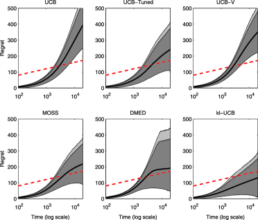
Figure 1: Regret of the various algorithms as a function of time (on a log-scale) in the Bernoulli ten-arm scenario. On each figure, the dashed line shows the asymptotic lower bound; the solid bold curve corresponds to the mean regret; while the dark and light shaded regions show, respectively, the central $99\%$ region and the upper $99.95\%$ quantile.

In Figure 1 we consider a difficult scenario, inspired by a situation (frequent in applications like marketing or Internet advertising) where the mean reward of each arm is very low. In our scenario, there are ten arms: the optimal arm has expected reward $0.1$, and the nine suboptimal arms consist of three different groups of three (stochastically) identical arms, each with respective expected rewards $0.05$, $0.02$ and $0.01$. We resorted to $N=50\mbox{,}000$ simulations to obtain the regret plots of Figure 1. These plots show, for each algorithm, the average cumulated regret together with quantiles of the cumulated regret distribution as a function of time (on a logarithmic scale).

Here, there is a huge gap in performance between UCB and kl-UCB. This is explained by the fact that the variances of all reward distributions are much smaller than $1/4$, the pessimistic upper bound used in Hoeffding’s inequality (i.e., in the design of UCB). The gain in performance of UCB-Tuned is not very significant. kl-UCB and DMED reach a performance that is on par with the lower bound (1) of Burnetas and Katehakis (1996) (shown in strong dashed line); the performance of kl-UCB is somewhat better than the one of DMED. Notice that for the best methods, and in particular for kl-UCB, the mean regret is below the lower bound, even for larger horizons, which reveals and illustrates the asymptotic nature of this bound.

7.2 Truncated Poisson rewards

In this second scenario, we consider $6$ arms with truncated Poisson distributions. More precisely, each arm $1\leq a\leq 6$ is associated with $\nu_{a}$, a Poisson distribution with expectation $(2+a)/4$, truncated at $10$. The experiment consisted of $N=10\mbox{,}000$ Monte Carlo replications on an horizon of $T=20\mbox{,}000$ steps. Note that the truncation does not alter much the distributions here, as the probability of draws larger than $10$ is small for all arms. In fact, the role of this truncation is only to provide an explicit upper bound on the possible rewards, which is required for most algorithms.

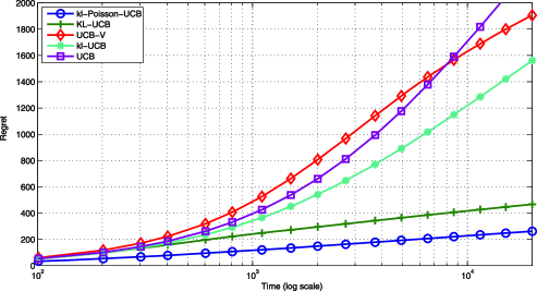
Figure 2: Regret of the various algorithms as a function of time in the truncated Poisson scenario.

Figure 2 shows that, in this case again, the UCB algorithm is significantly worse than some of its competitors. The UCB-V algorithm, which appears to have a larger regret on the first $5000$ steps, progressively improves thanks to its use of variance estimates for the arms. But the horizon $T=20\mbox{,}000$ is (by far) not sufficient for UCB-V to provide an advantage over kl-UCB, which is thus seen to offer an interesting alternative even in nonbinary cases.

These three methods, however, are outperformed by the kl-poisson-UCB algorithm: using the properties of the Poisson distributions (but not taking truncation into account, however), this algorithm achieves a regret that is about ten times smaller. In-between stands the empirical KL-UCB algorithm; it relies on nonparametric empirical-likelihood-based upper bounds and is therefore distribution-free as explained in Section 6.2, yet, it proves remarkably efficient.

7.3 Truncated exponential rewards

In the third and last example, there are $5$ arms associated with continuous distributions: the rewards are exponential variables, with respective parameters $1/5$, $1/4$, $1/3$, $1/2$ and $1$, truncated at $x_{\max}=10$ (i.e., they are bounded in $[0,10]$).

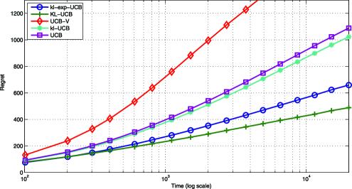
Figure 3: Regret of the various algorithms as a function of time in the truncated exponential scenario.

Figure 3 shows that in this scenario, UCB and MOSS are clearly suboptimal. This time, the kl-UCB does not provide a significant improvement over UCB as the expectations of the arms are not particularly close to $0$ or to $x_{\max}=10$; hence the confidence intervals computed by kl-UCB are close to those used by UCB. UCB-V, by estimating the variances of the distributions of the rewards, which are much smaller than the variances of $\{0,10\}$-valued distributions with the same expectations, would be expected to perform significantly better. But here again, UCB-V is not competitive, at least for a horizon $T=20\mbox{,}000$. This can be explained by the fact that the upper confidence bound of any suboptimal arm $a$, as stated in (16), contains a residual term $3\log(t)/N_{a}(t)$; this term is negligible in common applications of Bernstein’s inequality, but it does not vanish here because $N_{a}(t)$ is precisely of order $\log(t)$; see also Garivier and Cappé (2011) for further discussion of this issue.

The kl-exp-UCB algorithm uses the divergence $d(x,y)=x/y-1-\log(x/y)$ prescribed for genuine exponential distributions, but it ignores the fact that the rewards are truncated. However, contrary to the previous scenario, the truncation has an important effect here, as values larger than $10$ are relatively probable for each arm. Because kl-exp-UCB is not aware of the truncation, it uses upper bounds that are slightly too large; however, the performance is still excellent and stable, and the algorithm is particularly simple.

But the best-performing algorithm in this case is the nonparametric algorithm, empirical KL-UCB. This method appears to reach here the best compromise between efficiency and versatility, at the price of a larger computational complexity.

8 Conclusion

The kl-UCB algorithm is a quasi-optimal method for multi-armed bandits whenever the distributions associated with the arms are known to belong to a simple parametric family. For each one-dimensional exponential family, a specific divergence function has to be used in order to achieve the lower bound (1) of Lai and Robbins (1985).

However, the binary Kullback–Leibler divergence plays a special role: it is a conservative, universal choice for bounded distributions. The resulting algorithm is versatile, fast and simple and proves to be a significant improvement, both in theory and in practice, over the widely used UCB algorithm.

The more elaborate KL-UCB algorithm relies on nonparametric inference, by using the so-called empirical likelihood method. It is optimal if the distributions of the arms are only known to be bounded (with a known upper bound) and finitely supported. For general bounded arms, the empirical-likelihood-based upper confidence bounds, which are the core of the algorithm, still have an adequate level, but obtaining explicit finite-time regret bounds for the algorithm itself and/or reducing its computational complexity is still the object of further investigations; see the discussion in Section 6.2. The simulation results show that empirical KL-UCB is efficient in general cases when the distributions are far from being members of simple parametric families.

In a nutshell, empirical KL-UCB is to be preferred when the distributions of the arms are not known to belong (or be close) to a simple parametric family and when the kl-UCB algorithm is know not to get satisfactory performance—that is, for instance, when the variance of a $[0,1]$-valued arm with expectation $\mu$ is much smaller than $\mu(1-\mu)$.

Technical proofs [doi]10.1214/13-AOS1119SUPP .pdf aos1119_supp.pdf The supplemental article contains the proofs of the results stated in the paper.

References

- Agrawal (1995) {barticle}[mr] \bauthor\bsnmAgrawal, \bfnmRajeev\binitsR. (\byear1995). \btitleSample mean based index policies with regret for the multi-armed bandit problem. \bjournalAdv. in Appl. Probab. \bvolume27 \bpages1054–1078. \biddoi=10.2307/1427934, issn=0001-8678, mr=1358906 \bptokimsref \endbibitem
- Audibert and Bubeck (2010) {barticle}[mr] \bauthor\bsnmAudibert, \bfnmJean-Yves\binitsJ.-Y. and \bauthor\bsnmBubeck, \bfnmSébastien\binitsS. (\byear2010). \btitleRegret bounds and minimax policies under partial monitoring. \bjournalJ. Mach. Learn. Res. \bvolume11 \bpages2785–2836. \bidissn=1532-4435, mr=2738783 \bptokimsref \endbibitem
- Audibert, Munos and Szepesvári (2009) {barticle}[mr] \bauthor\bsnmAudibert, \bfnmJean-Yves\binitsJ.-Y., \bauthor\bsnmMunos, \bfnmRémi\binitsR. and \bauthor\bsnmSzepesvári, \bfnmCsaba\binitsC. (\byear2009). \btitleExploration-exploitation tradeoff using variance estimates in multi-armed bandits. \bjournalTheoret. Comput. Sci. \bvolume410 \bpages1876–1902. \biddoi=10.1016/j.tcs.2009.01.016, issn=0304-3975, mr=2514714 \bptokimsref \endbibitem
- Auer, Cesa-Bianchi and Fischer (2002) {barticle}[author] \bauthor\bsnmAuer, \bfnmP.\binitsP., \bauthor\bsnmCesa-Bianchi, \bfnmN.\binitsN. and \bauthor\bsnmFischer, \bfnmP.\binitsP. (\byear2002). \btitleFinite-time analysis of the multiarmed bandit problem. \bjournalMachine Learning \bvolume47 \bpages235–256. \bptokimsref \endbibitem
- Bubeck and Cesa-Bianchi (2012) {barticle}[author] \bauthor\bsnmBubeck, \bfnmS.\binitsS. and \bauthor\bsnmCesa-Bianchi, \bfnmN.\binitsN. (\byear2012). \btitleRegret analysis of stochastic and nonstochastic multi-armed bandit problems. \bjournalFoundations and Trends in Machine Learning \bvolume5 \bpages1–122. \bptokimsref \endbibitem
- Burnetas and Katehakis (1996) {barticle}[mr] \bauthor\bsnmBurnetas, \bfnmApostolos N.\binitsA. N. and \bauthor\bsnmKatehakis, \bfnmMichael N.\binitsM. N. (\byear1996). \btitleOptimal adaptive policies for sequential allocation problems. \bjournalAdv. in Appl. Math. \bvolume17 \bpages122–142. \biddoi=10.1006/aama.1996.0007, issn=0196-8858, mr=1390571 \bptokimsref \endbibitem
- Burnetas and Katehakis (1997) {barticle}[mr] \bauthor\bsnmBurnetas, \bfnmApostolos N.\binitsA. N. and \bauthor\bsnmKatehakis, \bfnmMichael N.\binitsM. N. (\byear1997). \btitleOptimal adaptive policies for Markov decision processes. \bjournalMath. Oper. Res. \bvolume22 \bpages222–255. \biddoi=10.1287/moor.22.1.222, issn=0364-765X, mr=1436581 \bptokimsref \endbibitem
- Burnetas and Katehakis (2003) {barticle}[mr] \bauthor\bsnmBurnetas, \bfnmApostolos N.\binitsA. N. and \bauthor\bsnmKatehakis, \bfnmMichael N.\binitsM. N. (\byear2003). \btitleAsymptotic Bayes analysis for the finite-horizon one-armed-bandit problem. \bjournalProbab. Engrg. Inform. Sci. \bvolume17 \bpages53–82. \biddoi=10.1017/S0269964803171045, issn=0269-9648, mr=1959385 \bptokimsref \endbibitem
- Cappé, Garivier and Kaufmann (2012) {bmisc}[author] \bauthor\bsnmCappé, \bfnmOlivier\binitsO., \bauthor\bsnmGarivier, \bfnmAurelien\binitsA. and \bauthor\bsnmKaufmann, \bfnmEmilie\binitsE. (\byear2012). \bhowpublishedpy/maBandits: Matlab and Python packages for multi-armed bandits. Available at http://mloss.org/software/ view/415/. \bptokimsref \endbibitem
- Cappé et al. (2013) {bmisc}[author] \bauthor\bsnmCappé, \bfnmO.\binitsO., \bauthor\bsnmGarivier, \bfnmA.\binitsA., \bauthor\bsnmMaillard, \bfnmO-A.\binitsO.-A., \bauthor\bsnmMunos, \bfnmR.\binitsR. and \bauthor\bsnmStoltz, \bfnmG.\binitsG. (\byear2013). \btitleSupplement to “Kullback–Leibler upper confidence bounds for optimal sequential allocation.” DOI:\doiurl10.1214/13-AOS1119SUPP. \bptokimsref \endbibitem
- Chang and Lai (1987) {barticle}[mr] \bauthor\bsnmChang, \bfnmFu\binitsF. and \bauthor\bsnmLai, \bfnmTze Leung\binitsT. L. (\byear1987). \btitleOptimal stopping and dynamic allocation. \bjournalAdv. in Appl. Probab. \bvolume19 \bpages829–853. \biddoi=10.2307/1427104, issn=0001-8678, mr=0914595 \bptokimsref \endbibitem
- Chow and Teicher (1988) {bbook}[mr] \bauthor\bsnmChow, \bfnmYuan Shih\binitsY. S. and \bauthor\bsnmTeicher, \bfnmHenry\binitsH. (\byear1988). \btitleProbability Theory: Independence, Interchangeability, Martingales, \bedition2nd ed. \bpublisherSpringer, \blocationNew York. \biddoi=10.1007/978-1-4684-0504-0, mr=0953964 \bptokimsref \endbibitem
- Dembo and Zeitouni (1998) {bbook}[mr] \bauthor\bsnmDembo, \bfnmAmir\binitsA. and \bauthor\bsnmZeitouni, \bfnmOfer\binitsO. (\byear1998). \btitleLarge Deviations Techniques and Applications, \bedition2nd ed. \bseriesApplications of Mathematics (New York) \bvolume38. \bpublisherSpringer, \blocationNew York. \bidmr=1619036 \bptokimsref \endbibitem
- Filippi, Cappé and Garivier (2010) {binproceedings}[author] \bauthor\bsnmFilippi, \bfnmS.\binitsS., \bauthor\bsnmCappé, \bfnmO.\binitsO. and \bauthor\bsnmGarivier, \bfnmA.\binitsA. (\byear2010). \btitleOptimism in reinforcement learning and Kullback–Leibler divergence. In \bbooktitleProceedings of the 48th Annual Allerton Conference on Communication, Control, and Computing. \bpublisherIEEE Press, \blocationPiscataway, NJ. \bptokimsref \endbibitem
- Garivier and Cappé (2011) {binproceedings}[author] \bauthor\bsnmGarivier, \bfnmA.\binitsA. and \bauthor\bsnmCappé, \bfnmO.\binitsO. (\byear2011). \btitleThe KL-UCB algorithm for bounded stochastic bandits and beyond. In \bbooktitleProceedings of the 24th Annual Conference on Learning Theory. \bpublisherJMLR C&WP. \bptokimsref \endbibitem
- Gittins (1979) {barticle}[mr] \bauthor\bsnmGittins, \bfnmJ. C.\binitsJ. C. (\byear1979). \btitleBandit processes and dynamic allocation indices (with discussion). \bjournalJ. R. Stat. Soc. Ser. B Stat. Methodol. \bvolume41 \bpages148–177. \bidissn=0035-9246, mr=0547241 \bptnotecheck related\bptokimsref \endbibitem
- Gittins, Glazebrook and Weber (2011) {bbook}[author] \bauthor\bsnmGittins, \bfnmJ.\binitsJ., \bauthor\bsnmGlazebrook, \bfnmK.\binitsK. and \bauthor\bsnmWeber, \bfnmR.\binitsR. (\byear2011). \btitleMulti-Armed Bandit Allocation Indices. \bpublisherWiley, \blocationNew York. \bptokimsref \endbibitem
- Hoeffding (1963) {barticle}[mr] \bauthor\bsnmHoeffding, \bfnmWassily\binitsW. (\byear1963). \btitleProbability inequalities for sums of bounded random variables. \bjournalJ. Amer. Statist. Assoc. \bvolume58 \bpages13–30. \bidissn=0162-1459, mr=0144363 \bptokimsref \endbibitem
- Honda and Takemura (2010) {binproceedings}[author] \bauthor\bsnmHonda, \bfnmJ.\binitsJ. and \bauthor\bsnmTakemura, \bfnmA.\binitsA. (\byear2010). \btitleAn asymptotically optimal bandit algorithm for bounded support models. In \bbooktitleProceedings of the 23rd Annual Conference on Learning Theory. \bpublisherOmnipress, \blocationMadison, WI. \bptokimsref \endbibitem
- Honda and Takemura (2011) {barticle}[author] \bauthor\bsnmHonda, \bfnmJ.\binitsJ. and \bauthor\bsnmTakemura, \bfnmA.\binitsA. (\byear2011). \btitleAn asymptotically optimal policy for finite support models in the multiarmed bandit problem. \bjournalMachine Learning \bvolume85 \bpages361–391. \bptokimsref \endbibitem
- Honda and Takemura (2012) {bmisc}[author] \bauthor\bsnmHonda, \bfnmJ.\binitsJ. and \bauthor\bsnmTakemura, \bfnmA.\binitsA. (\byear2012). \bhowpublishedFinite-time regret bound of a bandit algorithm for the semi-bounded support model. Available at \arxivurlarXiv:1202.2277. \bptokimsref \endbibitem
- Kaufmann, Cappé and Garivier (2012) {binproceedings}[author] \bauthor\bsnmKaufmann, \bfnmE.\binitsE., \bauthor\bsnmCappé, \bfnmO.\binitsO. and \bauthor\bsnmGarivier, \bfnmA.\binitsA. (\byear2012). \btitleOn Bayesian upper confidence bounds for bandit problems. In \bbooktitleProceedings of the 15th International Conference on Artificial Intelligence and Statistics 22 \bpages592–600. \bpublisherJMLR W&CP. \bptokimsref \endbibitem
- Kaufmann, Korda and Munos (2012) {binproceedings}[author] \bauthor\bsnmKaufmann, \bfnmE.\binitsE., \bauthor\bsnmKorda, \bfnmN.\binitsN. and \bauthor\bsnmMunos, \bfnmR.\binitsR. (\byear2012). \btitleThompson sampling: An asymptotically optimal finite time analysis. In \bbooktitleProceedings of the 23rd International Conference on Algorithmic Learning Theory \bpages199–213. \bpublisherSpringer, \blocationNew York. \bptokimsref \endbibitem
- Lai and Robbins (1985) {barticle}[mr] \bauthor\bsnmLai, \bfnmT. L.\binitsT. L. and \bauthor\bsnmRobbins, \bfnmHerbert\binitsH. (\byear1985). \btitleAsymptotically efficient adaptive allocation rules. \bjournalAdv. in Appl. Math. \bvolume6 \bpages4–22. \biddoi=10.1016/0196-8858(85)90002-8, issn=0196-8858, mr=0776826 \bptokimsref \endbibitem
- Lehmann and Casella (1998) {bbook}[mr] \bauthor\bsnmLehmann, \bfnmE. L.\binitsE. L. and \bauthor\bsnmCasella, \bfnmGeorge\binitsG. (\byear1998). \btitleTheory of Point Estimation, \bedition2nd ed. \bpublisherSpringer, \blocationNew York. \bidmr=1639875 \bptokimsref \endbibitem
- Maillard, Munos and Stoltz (2011) {binproceedings}[author] \bauthor\bsnmMaillard, \bfnmO-A.\binitsO.-A., \bauthor\bsnmMunos, \bfnmR.\binitsR. and \bauthor\bsnmStoltz, \bfnmG.\binitsG. (\byear2011). \btitleA finite-time analysis of multi-armed bandits problems with Kullback–Leibler divergences. In \bbooktitleProceedings of the 24th Annual Conference on Learning Theory. \bpublisherJMLR C&WP. \bptokimsref \endbibitem
- Massart (2007) {bbook}[mr] \bauthor\bsnmMassart, \bfnmPascal\binitsP. (\byear2007). \btitleConcentration Inequalities and Model Selection. \bseriesLecture Notes in Math. \bvolume1896. \bpublisherSpringer, \blocationBerlin. \bidmr=2319879 \bptokimsref \endbibitem
- Owen (2001) {bbook}[author] \bauthor\bsnmOwen, \bfnmA. B.\binitsA. B. (\byear2001). \btitleEmpirical Likelihood. \bpublisherChapman & Hall/CRC, \blocationBoca Raton, FL. \bptokimsref \endbibitem
- Robbins (1952) {barticle}[mr] \bauthor\bsnmRobbins, \bfnmHerbert\binitsH. (\byear1952). \btitleSome aspects of the sequential design of experiments. \bjournalBull. Amer. Math. Soc. (N.S.) \bvolume58 \bpages527–535. \bidissn=0002-9904, mr=0050246 \bptokimsref \endbibitem
- Thompson (1933) {barticle}[author] \bauthor\bsnmThompson, \bfnmW. R.\binitsW. R. (\byear1933). \btitleOn the likelihood that one unknown probability exceeds another in view of the evidence of two samples. \bjournalBiometrika \bvolume25 \bpages285–294. \bptokimsref \endbibitem
- Thompson (1935) {barticle}[mr] \bauthor\bsnmThompson, \bfnmWilliam R.\binitsW. R. (\byear1935). \btitleOn the Theory of Apportionment. \bjournalAmer. J. Math. \bvolume57 \bpages450–456. \biddoi=10.2307/2371219, issn=0002-9327, mr=1507085 \bptokimsref \endbibitem
- van der Vaart (2000) {bbook}[author] \bauthor\bparticlevan der \bsnmVaart, \bfnmA. W.\binitsA. W. (\byear2000). \btitleAsymptotic Statistics. \bpublisherCambridge Univ. Press, \blocationCambridge. \bptokimsref \endbibitem
- Wainwright and Jordan (2008) {barticle}[author] \bauthor\bsnmWainwright, \bfnmMartin J.\binitsM. J. and \bauthor\bsnmJordan, \bfnmMichael I.\binitsM. I. (\byear2008). \btitleGraphical models, exponential families, and variational inference. \bjournalFoundation and Trends in Machine Learning \bvolume1 \bpages1–305. \bptokimsref \endbibitem
- Wald (1945) {barticle}[mr] \bauthor\bsnmWald, \bfnmA.\binitsA. (\byear1945). \btitleSequential tests of statistical hypotheses. \bjournalAnn. Math. Statist. \bvolume16 \bpages117–186. \bidissn=0003-4851, mr=0013275 \bptokimsref \endbibitem
- Weber (1992) {barticle}[mr] \bauthor\bsnmWeber, \bfnmRichard\binitsR. (\byear1992). \btitleOn the Gittins index for multiarmed bandits. \bjournalAnn. Appl. Probab. \bvolume2 \bpages1024–1033. \bidissn=1050-5164, mr=1189430 \bptokimsref \endbibitem
- Whittle (1980) {barticle}[mr] \bauthor\bsnmWhittle, \bfnmP.\binitsP. (\byear1980). \btitleMulti-armed bandits and the Gittins index. \bjournalJ. R. Stat. Soc. Ser. B Stat. Methodol. \bvolume42 \bpages143–149. \bidissn=0035-9246, mr=0583348 \bptokimsref \endbibitem