Image reconstruction for observations with a high dynamic range: LINC-NIRVANA simulations of a stellar jet

Abstract

We report the results of a simulation and reconstruction of observations of a young stellar object (YSO) jet with the LINC-NIRVANA (LN) interferometric instrument, which will be mounted on the Large Binocular Telescope (LBT). This simulation has been performed in order to investigate the ability of observing the weak diffuse jet line emission against the strong IR stellar continuum through narrow band images in the H and K atmospheric windows. In general, this simulation provides clues on the image quality that could be achieved in observations with a high dynamic range. In these cases, standard deconvolution methods, such as Richardson-Lucy, do not provide satisfactory results: we therefore propose here a new method of image reconstruction. It consists in considering the image to be reconstructed as the sum of two terms: one corresponding to the star (whose position is assumed to be known) and the other to the jet. A regularization term is introduced for this second component and the reconstruction is obtained with an iterative method alternating between the two components. An analysis of the results shows that the image quality obtainable with this method is significantly improved with respect to standard deconvolution methods, reducing the number of artifacts and allowing us to reconstruct the original jet intensity distribution with an error smaller than 10%.

1 INTRODUCTION

The Large Binocular Telescope (LBT), currently operating on Mount Graham in Arizona, consists of two 8.4m mirrors on the same mount. This peculiar structure is particularly suited to perform Fizeau interferometry and, to this purpose, the near-infrared image-plane beam combiner LINC-NIRVANA (LN) is in an advanced stage of realization by an Italian-German consortium led by the Max Planck Institute for Astronomy in Heidelberg.

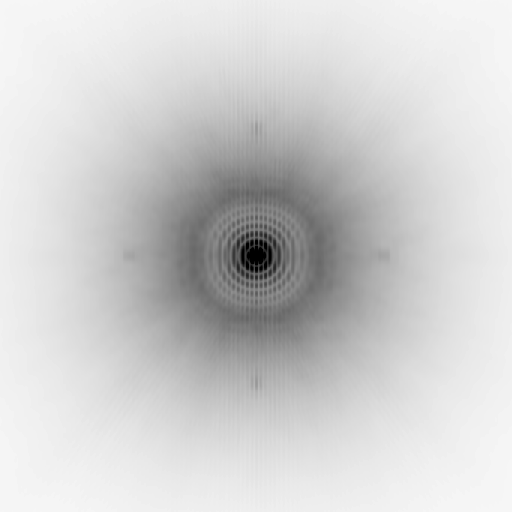
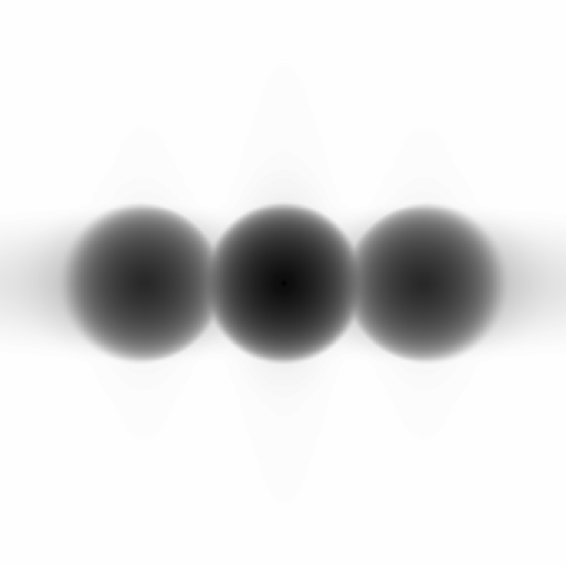
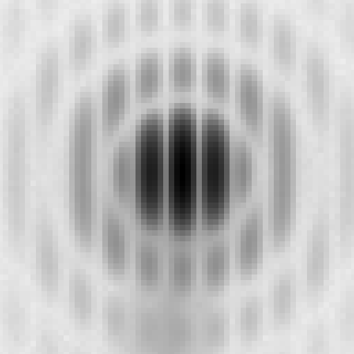
The performance of LN is expected to be close to the diffraction limit. Due to the binocular structure of the instrument, the Point Spread Function (PSF) may be described as the diffraction limited pattern of a 8.4m mirror crossed by the fringes due to the interference between the two apertures, with a maximum baseline of approximately 22.8m. In Fig. 1 we give an example of PSF with SR=0.7, obtained with the software LOST[1], together with its Modulus Transfer Function (MTF). Since the resolution of a given LN image is anisotropic, several images with different orientations of the baseline must be acquired and then processed (and combined) to obtain a final image with high resolution in all directions. For a discussion of the imaging problem for LINC-NIRVANA we refer to the review article by Bertero et al.[2].

Figure 1: Simulated PSF of LN with SR=70% (left panel), and the corresponding MTF (right panel). The fringes are orthogonal to the baseline. Both images are shown in log scale.

High angular resolution observations obtainable with an interferometer like LN are essential in the study of young jets, providing information on the magneto-hydrodynamical process that is at the origin and collimation of the jet. It is thus crucial to investigate the morphology of the jet in the close surroundings of the star, as the relevant physical processes are at work in the first 10 AU from the star, which correspond to about 70 mas (i.e. 14 pixels in our simulation) for objects in the nearest star-forming clouds at a distance of $\sim$150 pc. For this reason, it is of paramount importance to understand the goodness of the image reconstruction of the jet achievable by LN in the region around the star.

To this aim, in Ciliegi et al.[3], LN-images of a YSO model were generated using the software package AIRY-LN[4] and they were reconstructed using a multiple-image deconvolution method derived from the well known Richardson-Lucy (RL)[5, 6] iterative algorithm. However, the reconstruction of the jet was unsatisfactory in the region close to the emitting star, which is the most important for studying the physical process responsible for the launching and collimation of the jet. The main reason of this result is that standard deconvolution methods are unable to reconstruct an astronomical target consisting of a bright point-wise component (typically a star) superimposed to a weaker, diffuse component (in our case, the emitted jet). A bibliographical analysis of the methods proposed for solving this image reconstruction problem is provided by Giovannelli & Coulais[7]. In addition these authors propose, in the case of radio interferometry, an approach which consists in considering the object to be reconstructed as a superposition of two components, a point source and an extended source, and in introducing different regularization terms for the two components within a least-square approach to the problem. This is equivalent to assume an additive Gaussian noise.

In this paper we develop a similar idea but in the framework of Poisson noise where the standard image reconstruction method is RL. In the case of multiple image deconvolution, the problem arising in LINC-NIRVANA imaging, extensions of RL must be considered[2]. The method we propose will be denoted as multi-component Richardson-Lucy (MC-RL) method.

2 THE MC-RL METHOD

As stated in Sect. 1 we assume that the object to be reconstructed $f=f({\bf n})$, where ${\bf n}=\{n_{1},n_{2}\}$ is a multi-index labeling the pixels of the image, is the sum of two terms (or components), $f({\bf n})=f_{1}({\bf n})+f_{2}({\bf n})$, where $f_{1}$ corresponds to the point source and $f_{2}$ to the extended source. For simplicity we assume that the source is a single star whose position is known with a pixel precision, so that $f_{1}({\bf n})=c~{}\delta({\bf n},{\bf n}_{0})$, where ${\bf n}_{0}$ is the pixel where the star is located, $c$ is its unknown emission intensity and $\delta$ denotes the usual delta function. We first describe the approach in the case of single-image deconvolution; next we extend it to the case of multiple images.

2.1 Single-image deconvolution

As it is well-known, in the case of Poisson noise the negative logarithm of the likelihood is given, except for constant factors, by the Kullback-Leibler divergence, also known as Csiszár I-divergence[8]. Therefore, under the assumptions above, maximum likelihood (ML) solutions can be obtained by minimizing with respect to $f_{1},f_{2}$ the following function

$$J_{0}(f_{1},f_{2};g)=\sum_{{\bf n}\in S}\left\{g({\bf n}){\rm ln}\frac{g({\bf n})}{[A(f_{1}+f_{2})]({\bf n})+b({\bf n})}+[A(f_{1}+f_{2})]({\bf n})+b({\bf n})-g({\bf n})\right\}~{}~{},$$ (1)

where $b$ is the background emission (assumed to be known) and $A$ is the imaging matrix, which is given in terms of a space-invariant point spread function (PSF) $K$, normalized to unit volume, as follows

$$(Af)({\bf n})=(K*f)({\bf n})~{}~{},~{}~{}\sum_{{\bf n}\in S}K({\bf n})=1~{}~{}.$$ (2)

The function $J_{0}$ is nonnegative, convex and coercive in $f_{1},f_{2}$, as well as in their sum $f=f_{1}+f_{2}$ and therefore ML solutions exist. However, it is well-known that they appear as sky-night solutions[9], i.e. a set of bright spots over a black background. While this result can be satisfactory for the point source component, it is not for the extended source component. Therefore we add a regularization term for this one, a procedure which can be justified in the framework of a Bayesian approach. In conclusion, the function we intend to minimize has the following structure

$$J_{\mu}(f_{1},f_{2};g)=J_{0}(f_{1},f_{2};g)+\frac{\mu}{2}\sum_{{\bf n}\in S}|f_{2}({\bf n})|^{2}~{}~{},$$ (3)

where we assume a Tikhonov-like regularization and $\mu$ is a regularization parameter to be estimated. We discuss this point in the next section.

In order to extend RL to the minimization of this function with respect to $f_{1},f_{2}$, we must first compute its gradient with respect to these variables. We use the well-known expression of the gradient of $J_{0}(f;g)$, we denote as $\nabla_{1},\nabla_{2}$ the gradients with respect to $f_{1},f_{2}$, respectively, and finally, for simplifying the notation, we denote as $f$ their sum $f=f_{1}+f_{2}$. Using the normalization of the PSF it follows that

$$\nabla_{1}J_{\mu}(f_{1},f_{2};g)={\hat{1}}-A^{T}\frac{g}{Af+b}~{}~{},$$ (4)

$$\nabla_{2}J_{\mu}(f_{1},f_{2};g)={\hat{1}}-A^{T}\frac{g}{Af+b}+\mu f_{2}~{}~{},$$

where $\hat{1}$ is the array with all elements equal to 1 and the quotient of two arrays is intended pixel by pixel.

If we use, for instance, the split-gradient method (SGM)[10], then the iterative method for the minimization of $J_{\mu}$ is as follows: given $f_{1}^{(0)},f_{2}^{(0)}$, for $k=0,1,..$ compute

$$f_{1}^{(k+1)}=f_{1}^{(k)}A^{T}\frac{g}{Af^{(k)}+b}$$ (5)

$$f_{2}^{(k+1)}=\frac{f_{2}^{(k)}}{{\hat{1}}+\mu f_{2}^{(k)}}A^{T}\frac{g}{Af^{(k)}+b}$$

$$f^{(k+1)}=f_{1}^{(k+1)}+f_{2}^{(k+1)}~{}~{}.$$

It is easy to check by induction that, if we initialize the algorithm with $f_{1}^{(0)}({\bf n})=\delta({\bf n},{\bf n}_{0})$ (and $f_{2}^{(0)}$ arbitrary but positive) then, at iteration $k$, we have $f_{1}^{(k)}({\bf n})=c_{k}\delta({\bf n},{\bf n}_{0})$.

We do not have a proof of convergence of the previous algorithm, even if we have always found convergence in our numerical experiments. The algorithm is very slow, even slower than the standard RL algorithm. However, since it is a scaled gradient method, convergence and acceleration can be obtained in the framework of the so-called scaled gradient projection (SGP) method[11].

2.2 Multiple-image deconvolution

In the case of $p$ images, $g_{1},...,g_{p}$ (we denote as $g$ the set formed by these images), if we assume their statistical independence, then Eq. (1) is replaced by

$$J_{0}(f_{1},f_{2};g)=\sum_{j=1}^{p}\sum_{{\bf n}\in S}\left\{g_{j}({\bf n}){\rm ln}\frac{g_{j}({\bf n})}{[A_{j}(f_{1}+f_{2})]({\bf n})+b_{j}({\bf n})}+[A_{j}(f_{1}+f_{2})]({\bf n})+b_{j}({\bf n})-g_{j}({\bf n})\right\}~{}~{},$$ (6)

and the gradients of $J_{\mu}(f_{1},f_{2};g)$, defined as in Eq. (3), are given by

$$\nabla_{1}J_{\mu}(f_{1},f_{2};g)=p{\hat{1}}-\sum_{j=1}^{p}A_{j}^{T}\frac{g_{j}}{A_{j}f+b}~{}~{},$$ (7)

$$\nabla_{2}J_{\mu}(f_{1},f_{2};g)=p{\hat{1}}-\sum_{j=1}^{p}A_{j}^{T}\frac{g_{j}}{A_{j}f+b}+\mu f_{2}~{}~{}.$$

Therefore the algorithm (5) is replaced by: given $f_{1}^{(0)},f_{2}^{(0)}$, for $k=0,1,...$ compute

$$f_{1}^{(k+1)}=\frac{1}{p}f_{1}^{(k)}\sum_{j=1}^{p}A_{j}^{T}\frac{g_{j}}{A_{j}f^{(k)}+b}$$ (8)

$$f_{2}^{(k+1)}=\frac{f_{2}^{(k)}}{p{\hat{1}}+\mu f_{2}^{(k)}}\sum_{j=1}^{p}A_{j}^{T}\frac{g_{j}}{A_{j}f^{(k)}+b}$$

$$f^{(k+1)}=f_{1}^{(k+1)}+f_{2}^{(k+1)}~{}~{}.$$

The remarks concerning the algorithm (5) apply also to this one.

3 NUMERICAL EXPERIMENTS

3.1 Description of the observation simulation

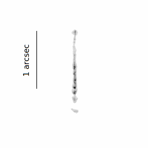
The synthetic image for our simulation has been obtained from an optical image taken with HST of the HH34 jet[12]. Starting from this image in Ciliegi et al.[3] the pixel scale was changed to the 5mas/pixel of LN and the integrated magnitude of the object was normalized to 13 mag in the H₂ band ($\lambda=2.12\mu m$, $\Delta\lambda=0.02\mu m$); moreover a point source having an H₂ magnitude of 13 mag was added at the position where the HH34 infrared driving source is located; finally, the average K-band sky brightness of 13.5 mag/arcsec² has been assumed as background emission.

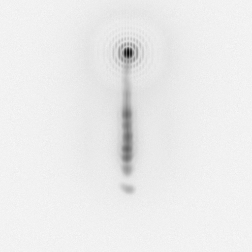
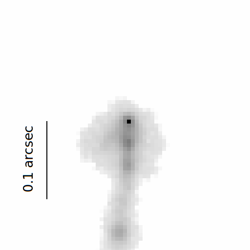
Four equispaced $1024\times 1024$ LN images, at $0^{\circ},~{}45^{\circ},~{}90^{\circ}$ and $135^{\circ}$, have been obtained by convolving the object with four PSFs generated through the software LOST[1]. The results are corrupted with Poisson and additive Gaussian noise with $\sigma=10\ e^{-}/$pixel. For each hour angle an integration time of 30 minutes has been chosen, for a total integration time of 2 hours. In Fig. 2 we show the object and one of the simulated LN-images.

Figure 2: The upper panels show the starting image of HH34 used for the simulations (left) and the simulated LN image at $0^{\circ}$ (right). The lower panels display a zoomed view of the region surrounding the star (left) and the corresponding part in the simulated image (right). The object images (left panels) are shown in sqrt scale, whereas the simulated LN observations (right panels) are in log scale.

3.2 Image deconvolution

The image deconvolution has been performed using the MC-RL method described in the previous section and, for comparison purposes, the standard Richardson-Lucy method for multiple images (RLM). In both cases, for the deconvolution process, we utilized the same PSFs used in convolution (inverse crime): in such a way we obtained the best reconstructed object available from the input data.

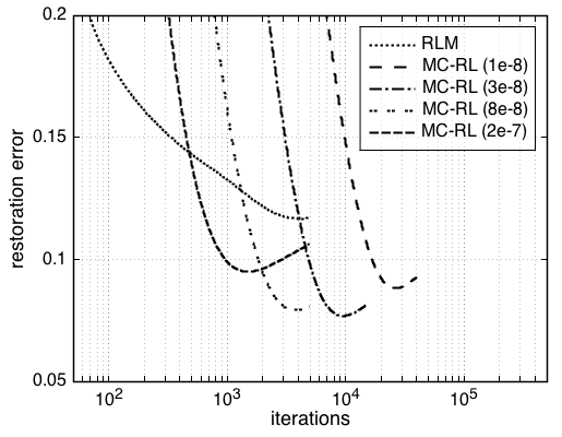
Since the two algorithms are iterative, early stopping of the iterations is required for obtaining sensible solutions. A stopping rule that can be used in numerical simulations, since we have the complete knowledge of the true object $\bar{f}$, consists in stopping the iteration when the relative r.m.s. error (also called restoration error), defined by

$$\rho^{(k)}=\frac{||f^{(k)}-\bar{f}||}{||\bar{f}||},$$ (9)

reaches a minimum value. As pointed out in Sect. 1, MC-RL is able to separately reconstruct the star and the diffuse part of the object, while RLM is not. For this reason, we computed the restoration error in two slightly different ways for the two algorithms:

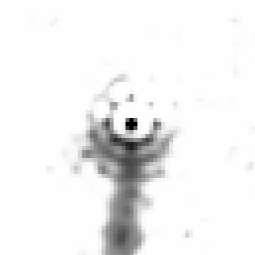
• RLM: we re-defined the true object $\bar{f}$ by using the image shown in the upper-left panel of Fig. 2 (i.e. the star superimposed to the jet) setting to 0 the values of the object in a 3$\times$3 region around the star position. In the same way we masked the reconstructed image before computing the restoration error.

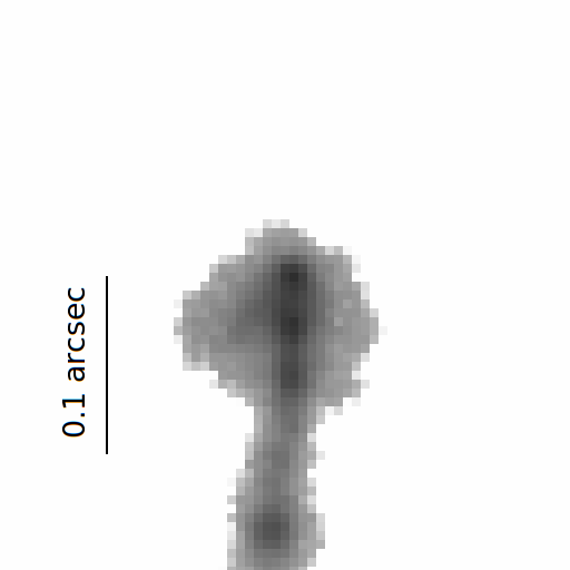
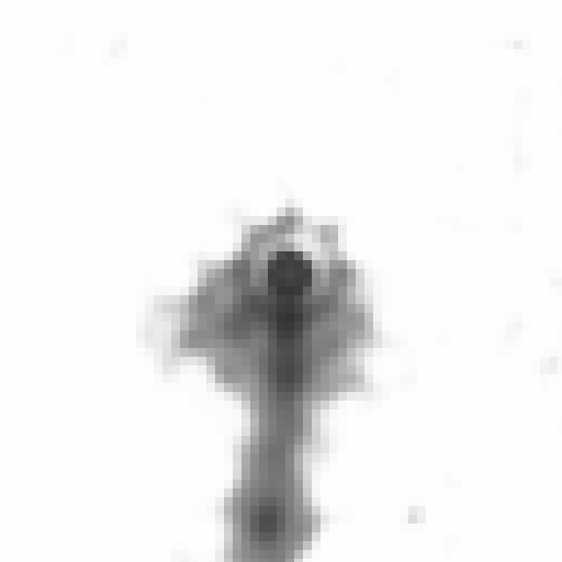
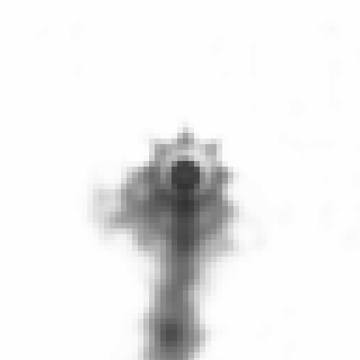
• MC-RL: we computed the restoration error by using $\bar{f}=\bar{f_{2}}$ (i.e. the diffuse jet without the star) as shown in Fig. 4.

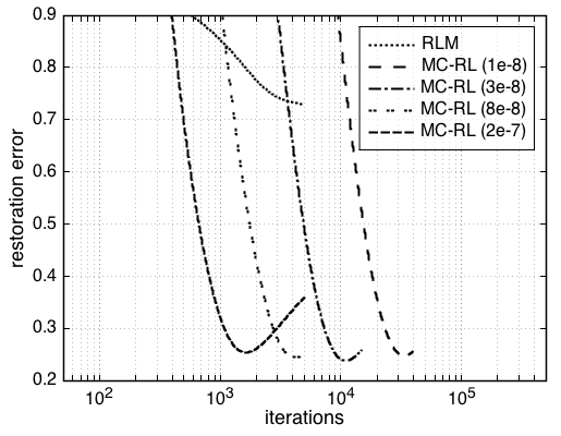
Moreover, since the astrophysical interest for this kind of object is focused on the region close to the star (where formation and collimation of the jet occur, see Sect. 4), we computed two different restoration errors: the former (indicated by $\rho^{\prime}$) by considering the entire jet, the latter ($\rho^{\prime\prime}$) by considering only 24 rows of the image around the star position.

As concerns the MC-RL method, the choice of the regularization parameter $\mu$ can be performed by minimizing the restoration error defined in the previous equation. For the values of $\mu$=$2\cdot 10^{-7}$, $8\cdot 10^{-8}$, $3\cdot 10^{-8}$, and $1\cdot 10^{-8}$, we plot in Fig. 3 the two restoration errors $\rho^{\prime}$ and $\rho^{\prime\prime}$ as functions of the number of iterations. In addition, we also plot the restoration errors of the reconstructed object obtained by RLM. We report the minimum values and the number of iterations at which they occur in Tab. 1.

Figure 3: The restoration error $\rho^{\prime}$ of the entire jet (left panel), and the restoration error $\rho^{\prime\prime}$ of the small region close to the star (right panel). Both errors are a function of the number of iterations.

Method	$\rho^{\prime}$ (nb of iterations)	$\rho^{\prime\prime}$ (nb of iterations)
RLM	11.67% (4251)	72.87% ($>5000$)
MC-RL ($\mu=1\cdot 10^{-8}$)	8.82% (26614)	24.80% (33483)
MC-RL ($\mu=3\cdot 10^{-8}$)	7.68% (9503)	23.81% (10972)
MC-RL ($\mu=8\cdot 10^{-8}$)	7.91% (3776)	24.42% (4198)
MC-RL ($\mu=2\cdot 10^{-7}$)	9.49% (1496)	25.34% (1630)

Table 1: The minimum values of the restoration errors $\rho^{\prime}$ and $\rho^{\prime\prime}$ and the corresponding number of iterations.

4 DATA ANALYSIS

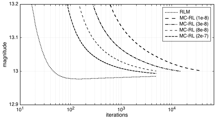
In Fig. 4 we show the reconstructed object for the RLM case and for the MC-RL cases with different values of $\mu$. More precisely, a magnification of the part of the jet close to the star is shown. These images correspond to the reconstructions obtained with the number of iterations that provides the minimum value of $\rho^{\prime\prime}$ (see Table 1). Moreover, in Fig. 5 we show the magnitude of the reconstructed star as a function of the number of iterations. The star flux has been computed in a 3$\times$3 box centered on its known position. Although there are small differences between RLM and MC-RL, both algorithms provide the correct value (13 mag) with satisfactory precision. Moreover, RLM reaches this value after a smaller number of iterations than the MC-RL method.

True object	RLM	MC-RL ($\mu=1\cdot 10^{-8}$)
MC-RL ($\mu=3\cdot 10^{-8}$)	MC-RL ($\mu=8\cdot 10^{-8}$)	MC-RL ($\mu=2\cdot 10^{-7}$)

Figure 4: The true object, the reconstructed object obtained with RLM, and the reconstructions with MC-RL for different values of the regularization parameter $\mu$.

Figure 5: The magnitude of the reconstructed star for RLM and MC-RL. All reconstructions provide the correct magnitude (m=13) of the star, with errors smaller than 0.1 mag.

However, as remarked in Sect.1, it is very important to investigate the morphology of the jet in the close surroundings of the star and, for this reason, we need to obtain a good image reconstruction of the jet in the region around the star. In this context, the significant difference that we find for the restoration error $\rho^{\prime\prime}$ (see Tab. 1) already indicates that the MC-RL method works much better than the standard RLM. Of course, since the restoration error provides only an indication of the global quality of the reconstructions, a more detailed analysis requires a direct comparison of the object morphology in the original and reconstructed images. Indeed, a quick look at Fig. 4 clearly shows that the region around the star is significantly less affected by artifacts when using the MC-RL method, confirming the result indicated by $\rho^{\prime\prime}$.

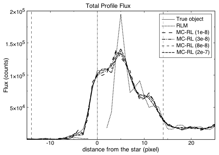
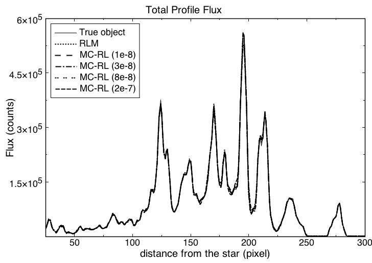
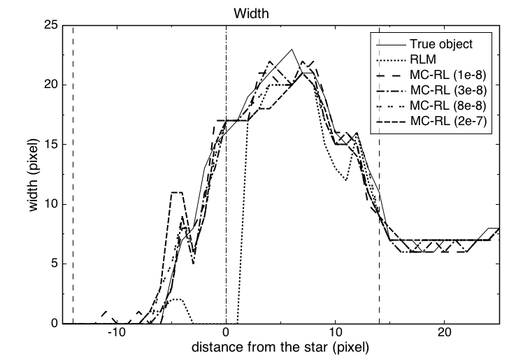
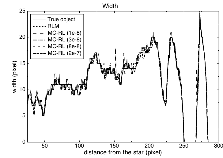
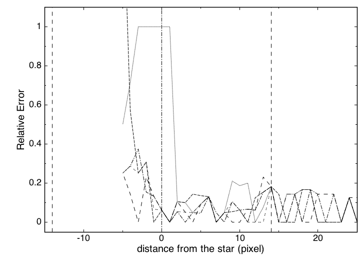
In order to compare the different methods, we have tried to quantify the quality of the reconstructions by taking into account two additional parameters: the integrated flux in the direction perpendicular to the jet axis (total profile flux) and the jet width. The first one is simply the flux obtained by summing up each pixel line of the image, as the jet is oriented along the y-axis of the image itself. As for the width computation, we cannot use a Gaussian FWHM, since the profile of the jet is in general not Gaussian. Hence, we set an arbitrary count threshold and define the width of the jet as the number of pixels lying between the first and the last pixel (along the considered line) that have a number of counts greater than the threshold. We note that the width is a key parameter for the scientific analysis, since it is directly related to the measurement (to be performed as close as possible to the exciting source) of the collimation of the jet.

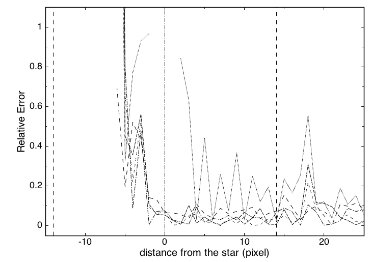
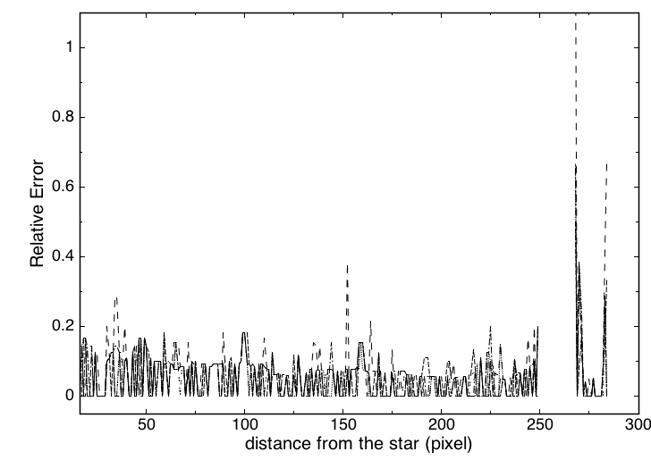
We analyze the total profile flux (shown in Fig. 6) and width (Fig. 7) as a function of the position along the jet and directly compare the values measured on the original image to the ones obtained for RLM and MC-RL images. In particular, we show the differences with respect to the original image in terms of the relative error on the parameter values. For each parameter we have used two separate series of plots: one for the region around the star, covering $\sim$200 mas (40 pixels), and the other including the rest of the jet.

Figure 6: Comparison of the integrated jet profile flux as measured in the original object image (solid thick line) and in the various reconstruction methods considered (RLM and MC-RL with different values of $\mu$, see legend) as a function of the position along the jet axis. The visualization is split in two plots: one for the region around the star (left panels), covering $\sim$40 pixels, and the other including the remaining part of the jet (right panels). The position of the star is marked by the vertical dashed-dotted line, while the dashed vertical lines delimit the typical region of interest for the formation and collimation of the jet (within $\sim$10 AU from the star) in the case of an object at a distance of 150 pc. The differences between the parameter values measured in the original image and in each reconstructed image are displayed in terms of relative errors in the bottom panels. In order to compare the jet reconstruction obtained through RLM (containing the star) and the results from MC-RL (where the star is not present), we have masked the 3 pixel lines around the position of the star in the RLM image.

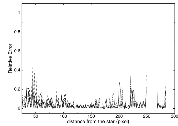The plots show that in the jet region both RLM and MC-RL methods provide a fairly good reconstruction of the image, with relative errors typically below 10% for both total profile flux and width. We note that MC-RL with the lowest and highest $\mu$ values ($1\cdot 10^{-8}$ and $2\cdot 10^{-7}$) give somewhat larger relative errors for the profile flux (peaks up to $\sim$20%-30%), so that intermediate $\mu$ values appear to work better.

In the star region the RLM shows instead much higher relative errors for the total profile flux (40%-60%) because of the artifacts, whereas MC-RL reconstructions are characterized by errors that are on average around 10% only. As for the width measurement, the best reconstructions are again obtained using the MC-RL algorithm with intermediate values of $\mu$ ($\mu=8\cdot 10^{-8}$ and $\mu=3\cdot 10^{-8}$), for which we get errors of about 10% in proximity of the star.

To summarize, our analysis shows that the use of the MC-RL algorithm allows us to limit the number and intensity of the artifacts in the region around the star. In the case examined, intermediate values of the regularization parameter $\mu$ provide the most accurate reconstruction of the original image. This shows that the MC-RL method can provide optimal results through a fine-tuning of this parameter.

Figure 7: Comparison of jet width as measured in the original object image (solid thick line) and in the various reconstruction methods considered (RLM and MC-RL with different values of $\mu$, see legend) as a function of the position along the jet axis. The visualization is split in two plots: one for the region around the star (left panels), covering $\sim$40 pixels, and the other including the remaining part of the jet (right panels). The position of the star is marked by the vertical dashed-dotted line, while the dashed vertical lines delimit the typical region of interest for the formation and collimation of the jet (within $\sim$10 AU from the star) in the case of an object at a distance of 150 pc. The differences between the parameter values measured in the original image and in each reconstructed image are displayed in terms of relative errors in the bottom panels.

5 CONCLUSIONS

We have simulated the observations and image reconstructions of a YSO jet with the LBT/LINC-NIRVANA interferometric instrument. This is a typical case of high dynamic range observations (weak diffuse jet line emission superimposed to a strong stellar continuum) in which standard deconvolution methods, such as Richardson-Lucy, do not provide satisfactory results. We have therefore proposed and analyzed a new method of image reconstruction, which we call multi-component Richardson-Lucy (MC-RL), in which we consider the image to be reconstructed as the sum of two terms (star plus jet). A regularization parameter is introduced for this second component and the reconstruction is obtained with an iterative method alternating between the two components.

Our main conclusions can be summarized as follows:

• The proposed MC-RL method works better than the standard RL method since it is able to effectively reduce artifacts in the star region, which is the most important one in the light of the scientific aim of the simulated observations, that is the study of the formation and collimation of the jet.

• For both methods the computational cost per iteration is high since one has to manage four 1024$\times$1024 LN-images. Therefore it is important to increase the efficiency of the algorithm by reducing the number of iterations. To this purpose the SGP approach proposed by Bonettini et al. [11] seems to be quite promising.

• The choice of a suitable value of the regularization parameter $\mu$ is an important issue. In this paper the parameter is estimated by searching for a minimum of the r.m.s. error. The value we found is also providing the best results for what concerns the measurements of both the flux and width of the jet, as confirmed by our comparison of the original and reconstructed images. We therefore show that the value of $\mu$ can be successfully fine-tuned in our simulations, although the problem of estimating the optimal value of $\mu$ might not be trivial in the case of real data.

• Besides this problem it is necessary to evaluate the robustness of the method with respect to errors in the estimate of the position of the star and evaluate its accuracy as a function of the relative magnitude of the star and the surrounding jet.

• Finally, the method can be easily extended to the case of several stars superimposed to smoothly varying objects, provided the positions of the stars can be estimated with sufficient accuracy.

• As a future development of this work, we plan to investigate the results provided by the MC-RL method when the contrast between star and jet is even higher, which is often the case for real objects in the sky.