Tidal disruption flares from stars on eccentric orbits

Abstract

We study tidal disruption and subsequent mass fallback for stars approaching supermassive black holes on bound orbits, by performing three dimensional Smoothed Particle Hydrodynamics simulations with a pseudo-Newtonian potential. We find that the mass fallback rate decays with the expected -5/3 power of time for parabolic orbits, albeit with a slight deviation due to the self-gravity of the stellar debris. For eccentric orbits, however, there is a critical value of the orbital eccentricity, significantly below which all of the stellar debris is bound to the supermassive black hole. All the mass therefore falls back to the supermassive black hole in a much shorter time than in the standard, parabolic case. The resultant mass fallback rate considerably exceeds the Eddington accretion rate and substantially differs from the -5/3 power of time.

1 Introduction

There is substantial evidence that galactic nuclei harbor supermassive black holes (SMBHs), the majority of which are quiescent and not active galactic nuclei. The tidal disruption of a star by a SMBH, and subsequent flaring activity, provides a rare observational diagnosis for the large population of quiescent SMBHs. These powerful flares are expected to have a luminosity at least comparable to the Eddington luminosity rmj88 ; sq09 .

The standard picture of a tidal disruption event (TDE) involves a star at large separation falling into a massive black hole on an almost parabolic orbit. After the star is tidally disrupted by the SMBH, half the stellar debris becomes gravitationally bound to the SMBH as it loses orbital energy inside the tidal radius. The bound debris finally falls back and accretes onto the black hole. Kepler’s third law implies that the accretion rate decays with the -5/3 power of time rmj88 ; ecr89 .

Observed light curves are in reasonable agreement with this theoretically predicted mass fallback rate, although some show deviations gs12 and the sample size is sufficiently small to make detailed testing of theoretical models difficult. Observations suggest that the TDE rate is $\sim 10^{-5}\rm{yr}^{-1}$ per galaxy djl02 . This observed rate is in rough agreement with theoretical rate estimates based on two-body scattering at $\sim\rm{pc}$ scales, which motivates the assumption of nearly parabolic orbits mt99 .

However, recent theoretical studies on rates of tidal separation of binary stars by SMBHs suggest that a significant fraction of tidal disruption flares may occur from stars approaching the black hole on somewhat eccentric orbits, significantly less parabolic than in the standard picture asp11 . Other sources of TDEs from stars on more eccentric orbits include binary SMBH systems and recoiling SMBHs kh12 . These latter two sources are capable of producing TDEs with even lower values of orbital eccentricity than in the binary separation scenario, and motivate our work here. In this paper, we explore through hydrodynamical simulations how mass fallback rates in TDEs vary between the canonical, parabolic case and the underexplored eccentric scenario.

2 Numerical method

We describe here procedures for numerically modeling the tidal disruption of stars on bound orbits. The simulations presented below were performed with a three-dimensional (3D) Smoothed Particle Hydrodynamics (SPH) code, which is based on a version originally developed by Ref. bate95 . We model the initial star as a polytropic gas sphere in hydrostatic equilibrium. The tidal disruption process is then simulated by setting the star in motion through the gravitational field of an SMBH.

A star is tidally disrupted when the tidal force of the black hole acting on the star is stronger than the star’s self-gravity. The radius where these two forces balance is defined as the tidal disruption radius

$$r_{\rm t}=\left(\frac{M_{\rm BH}}{m_{*}}\right)^{1/3}r_{*},$$ (1)

where $M_{\rm{BH}}$ is the black hole mass and $m_{*}$ is the stellar mass. The star-black hole system is put on the $x$-$y$ plane, where both axes are normalized by $r_{\rm{t}}$ and the black hole is put at the origin of the system. The initial position of the star is given by $\mbox{\boldmath$r$}_{0}=(r_{\rm 0}\cos\phi_{0},r_{\rm 0}\sin\phi_{0},0)$, where $r_{0}=3r_{\rm{t}}$ is the radial distance from the black hole and $\phi_{0}$ shows the angle between $x$-axis and $\mbox{\boldmath$r$}_{0}$. In our simulations, the black hole is represented by a sink particle with the appropriate gravitational mass $M_{\rm{BH}}$. All gas particles that fall within a specified accretion radius are accreted by the sink particle. We set the accretion radius of the black hole as equal to the Schwarzshild radius $r_{\rm{S}}=2GM_{\rm{BH}}/c^{2}$, with $c$ being the speed of light.

In order to treat approximately the relativistic precession of a test particle in the Schwarzschild metric, we incorporate into our SPH code the following pseudo-Newtonian potential wc12 :

$$U(r)=-\frac{GM_{\rm{BH}}}{r}\left[c_{1}+\frac{1-c_{1}}{1-c_{2}(r_{\rm{S}}/2r)}+c_{3}\frac{r_{\rm{S}}}{2r}\right],$$ (2)

where we adopt $c_{1}=(-4/3)(2+\sqrt{6})$, $c_{2}=(4\sqrt{6}-9)$, and $c_{3}=(-4/3)(2\sqrt{6-3})$. Equation (2) reduces to the Newtonian potential when $c_{1}=1$ and $c_{2}=c_{3}=0$ are adopted. Note that equation (2) includes no higher-order relativistic effects such as the black hole spin or gravitational wave emission.

We have performed five simulations of tidal disruption events with different parameters. The common parameters through all of simulations are following: $m_{*}=1M_{\odot}$, $r_{*}=1R_{\odot}$, $M_{\rm{BH}}=10^{6}M_{\odot}$, $\phi_{0}=-0.4\pi$, and $\gamma=5/3$. The total number of SPH particles used in each simulation is $10^{5}$, and the termination time of each simulation is $4\Omega_{*}^{-1}$, where $\Omega_{*}^{-1}\equiv\sqrt{r_{*}^{3}/Gm_{*}}\simeq 5.1\times 10^{-5}(r_{*}/R_{\odot})^{3/2}(M_{\odot}/m_{*})^{1/2}\,\rm{yr}$. We also adopt standard SPH artificial viscosity parameters $\alpha_{\mathrm{SPH}}=1$ or $\beta_{\mathrm{SPH}}=2$. Table 1 summarizes each model, where the penetration factor $\beta$ represents the ratio of the tidal disruption radius to pericenter distance, $r_{\rm{p}}$.

3 Tidal disruption of stars on bound orbits

As an approaching star enters into the tidal disruption radius, its fluid elements become dominated by the tidal force of the black hole, while their own self-gravity and pressure forces become relatively negligible. The tidal force then produces a spread in specific energy of the stellar debris

$$\Delta\epsilon\approx\frac{GM_{\rm{BH}}r_{*}}{r_{\rm t}^{2}}.$$ (3)

The total mass of the stellar debris is defined with the differential mass distribution $m(\epsilon)\equiv dM(\epsilon)/d\epsilon$, where $M(\epsilon)\equiv\int_{-\infty}^{\infty}m(\epsilon^{{}^{\prime}})d\epsilon^{{}^{\prime}}$. When a star is disrupted from a parabolic orbit, $m(\epsilon)$ will be centered on zero and distributed over $-\Delta\epsilon\leq\epsilon\leq\Delta\epsilon$.

Since the stellar debris with negative specific energy is bound to the SMBH, it returns to pericenter and will eventually accrete onto the black hole. If we define its binding energy, $\epsilon=-GM_{\rm{BH}}/2a$ (the semi-major axis of the stellar debris is $a$), then the mass fallback rate is given by ecr89 $dM/dt=(dM(\epsilon)/d\epsilon)|d\epsilon/dt|\,\,(\epsilon<0)$, where $d\epsilon/dt=-(1/3)(2\pi{GM_{\rm{BH}}})^{2/3}t^{-5/3}$. This is derived from Kepler’s third law.

Table 1: The first column shows each simulated scenario. The second, third, and fourth columns are the penetration factor $\beta=r_{\rm{p}}/r_{\rm{T}}$, the initial orbital eccentricity of star-black hole system $e_{*}$, and its initial semi-major axis $a_{*}$, respectively. The last column describes the remark for each model.

Model	$\beta=r_{\rm{t}}/r_{\rm{p}}$	$e_{*}$	$a_{*}\,[r_{\rm{t}}]$	Remarks
1	$1$	$1.0$	$-$	Newtonian
2	$1$	$1.0$	$-$	Pseudo-Newtonian
3	$5$	$1.0$	$-$	Pseudo-Newtonian
4	$1$	$0.98$	$50.0$	Pseudo-Newtonian
5	$5$	$0.98$	$10.0$	Pseudo-Newtonian

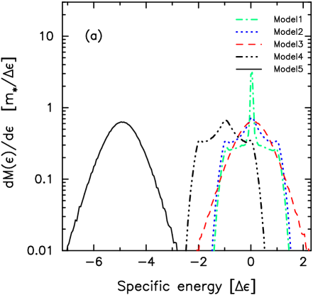
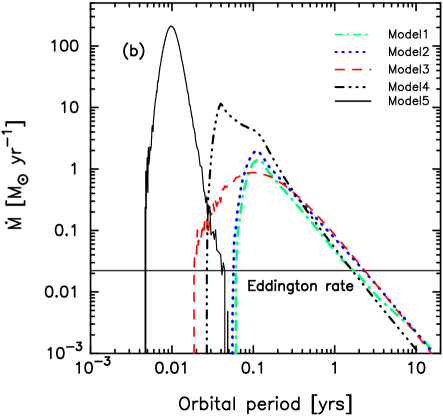
Figure 1: Differential mass distributions over specific energy of stellar debris and their corresponding mass-fall back rates. While the differential mass distribution is shown in panel (a), the mass fallback rate is shown in panel (b). In both panels, the dot-dashed line (green), dotted line (blue), dashed line (red), dashed-three-dotted line (black), and solid line (black) represent the mass distributions and corresponding mass fallback rates of Model 1, Model 2, Model 3, Model 4 and Model 5, respectively. The energy is measured in units of $\Delta\epsilon$ given by equation (3).

The specific orbital energy of a star on an eccentric orbit is given by

$$\epsilon_{\rm{orb}}\approx-\frac{GM_{\rm{BH}}}{2a_{*}}=-\frac{GM_{\rm{BH}}}{2r_{\rm{t}}}\beta(1-e_{*}),$$ (4)

where $a_{*}$ and $e_{*}$ are the initial semi-major axis of the star-black hole system and its initial orbital eccentricity, respectively. This quantity is less than zero because of the finite value of $a_{*}$, in contrast to the standard, parabolic orbit of a star. If $\epsilon_{\rm{orb}}$ is less than $\Delta\epsilon$, all the stellar debris should be bounded by the black hole, even after the tidal disruption. The condition $\epsilon_{\rm{orb}}=\Delta\epsilon$ therefore gives a critical value of orbital eccentricity of the star

$$e_{\rm crit}\approx 1-\frac{2}{\beta}\left(\frac{m_{*}}{M_{\rm BH}}\right)^{1/3},$$ (5)

below which all the stellar debris should remain gravitationally bound to the black hole. The critical eccentricity is evaluated to be $e_{\rm{crit}}=0.98$ for Model 4, whereas $e_{\rm{crit}}=0.996$ for Model 5. For the eccentric TDEs, the orbital period of the most tightly bound orbit, $t_{\rm{min}}$, and the orbital period of the most loosely bound orbit, $t_{\rm{max}}$, are obtained by using Kepler’s third law with $\epsilon=\Delta\epsilon\pm\epsilon_{\rm{orb}}$ and equation (4). The duration time of mass fallback for eccentric TDEs with $e_{*}<e_{\rm{crit}}$ is thus predicted to be finite and can be written by $\Delta{t}=t_{\rm{max}}-t_{\rm{min}}=(\pi/\sqrt{2})(\Omega_{*}^{-1}/[\beta(1-e_{*})]^{3/2})\left(\left[1/2-(1/\beta(1-e_{*})(m_{*}/M_{\rm{BH}})^{1/3}\right]^{-3/2}-1\right).$ Evaluating this gives $\Delta{t}\approx 207\Omega_{*}^{-1}$ for Model 5, whereas $\Delta{t}\rightarrow\infty$ for Model 4 in spite of smaller $t_{\rm{min}}$ than that of Models 1-3.

Figure 1 show differential mass distributions and their corresponding mass fallback rates in Models 1-5. While the differential mass distribution is shown in panel (a), the mass fallback rate is shown in panel (b). In panel (b), the horizontal solid line denotes the Eddington rate: $\dot{M}_{\rm{Edd}}=(1/\eta)(L_{\rm{Edd}}/c^{2})\simeq 2.2\times 10^{-2}(\eta/0.1)^{-1}(M_{\rm{BH}}/10^{6}M_{\odot})\,\,M_{\odot}\rm{yr^{-1}}$, where $L_{\rm{Edd}}=4\pi GM_{\rm{BH}}m_{\rm{p}}c/\sigma_{\rm{T}}$ is the Eddington luminosity with $m_{\rm{p}}$ and $\sigma_{\rm{T}}$ denoting the proton mass and Thomson scattering cross section, respectively, and $\eta$ is the mass-to-energy conversion efficiency, which is set to $0.1$ in the following discussion.

In panel (a), the central peak of Model 1 is attributed to mass congregation, from the self-gravity of the stellar debris. The energy spread corresponds to $\Delta\epsilon$ before and after the tidal disruption. The corresponding mass fallback rates are proportional to $t^{-5/3}$. The slight deviation from time to the $-5/3$ power originates from the convexity around $\Delta\epsilon$ and the central peak rising from $0.2\Delta\epsilon$ to $0$ (see also lg09 ). Simulations of Models 2 and 3 have performed with the pseudo-Newtonian potential given by equation (2). Model 3 has the same simulation parameters as Model 2 except for $\beta=5$. Since the potential is deeper as $\beta$ is higher, the re-congregation of the mass due to the self-gravity of the stellar debris is prevented. This leads to the mildly-sloped mass distribution, and therefore the peak of the mass fallback rate also smooths.

The mass is not distributed around zero but around $-\Delta\epsilon$ in Model 4, and around $-5\Delta\epsilon$ in Model 5. This is because the specific energy of initial stellar orbit is originally negative (see equation 4). Clearly, most of mass in Model 4 is bounded by the negative shift of the center. The resultant energy spread is slightly larger than we analytically expected. This suggests that the critical eccentricity is smaller than the value in equation (5). In Model 5, all of mass is bounded and falls back to the black hole in a much shorter time than that of Models 1-3. As shown in panel (b), the mass fallback rate of Model 5 is four orders of magnitude greater than the Eddington rate.

4 Concluding remarks

We have performed 3D SPH simulations of tidal disruption processes for stars on bound orbits. Our main conclusions are summarized as follows:

1. There is a critical orbital eccentricity below which all stellar debris falls back to the black hole. The simulated critical eccentricity is slightly lower than expected from our analytical prediction.

2. In an eccentric TDE with orbital eccentricity below the critical eccentricity, all the stellar debris falls back to the black hole in a much shorter time than that of the standard TDE. The resultant mass fallback rate substantially exceeds the Eddington rate and differs from the -5/3 power of time.

The full details of this work can be seen in Ref. kh12 .

References

- (1) Rees M. J, Nature 333, (1988) 523
- (2) Strubbe, L. E., Quataert, E., 2009, MNRAS, 400, 2070
- (3) Evans C.R, & Kochanek C.S, ApJ 346, (1989) L13
- (4) Gezari S., et al, Nature 485, (2012) 217
- (5) Donley J. L., Brandt W. N., Eracleous M., Boller T., 2002, AJ, 124, 1308
- (6) Magorrian, J., Tremaine, S., 1999, MNRAS, 309, 447
- (7) Amaro-Seoane, P., Coleman Miller, M., Kennedy, F. G, arXiv:1106.1429 (2011)
- (8) Hayasaki, K., Nicholas, S, & Loeb, A, submitted to MNRAS, (2012)
- (9) Bate, M. R., Bonnel, I. A., & Price, N.M, MNRAS 277, (1995) 362
- (10) Wegg C., 2012, ApJ, 749, 183
- (11) Lodato G, King A. R, & Pringle J. E, MNRAS 392, (2009) 332