Towards accelerating Smoothed Particle Hydrodynamics simulations
for free-surface flows on multi-GPU clusters

Abstract

Starting from the single graphics processing unit (GPU) version of the Smoothed Particle Hydrodynamics (SPH) code DualSPHysics, a multi-GPU SPH program is developed for free-surface flows. The approach is based on a spatial decomposition technique, whereby different portions (sub-domains) of the physical system under study are assigned to different GPUs. Communication between devices is achieved with the use of Message Passing Interface (MPI) application programming interface (API) routines. The use of the sorting algorithm radix sort for inter-GPU particle migration and sub-domain “halo” building (which enables interaction between SPH particles of different sub-domains) is described in detail. With the resulting scheme it is possible, on the one hand, to carry out simulations that could also be performed on a single GPU, but they can now be performed even faster than on one of these devices alone. On the other hand, accelerated simulations can be performed with up to 32 million particles on the current architecture, which is beyond the limitations of a single GPU due to memory constraints. A study of weak and strong scaling behaviour, speedups and efficiency of the resulting program is presented including an investigation to elucidate the computational bottlenecks. Last, possibilities for reduction of the effects of overhead on computational efficiency in future versions of our scheme are discussed.

1 Introduction

The applicability of particle-based simulations is typically limited by two different but related computational constraints: simulation time and system size. That is, to obtain physically meaningful information from a simulation, one must be able to simulate a large-enough system for long-enough times. In the particular case of the Smoothed Particle Hydrodynamics (SPH) method, certain types of applications, for example the study of coastal processes and flooding hydrodynamics, have been limited until now by the maximum number of particles in order to perform simulations within reasonable times.

To overcome these limitations, various types of acceleration techniques have been employed, which can be grouped into three main categories based on the type of hardware used. On the one hand there are the traditional High Performance Computing (HPC) techniques which involve the use of hundreds or thousands of computing nodes, each hosting one or more Central Processing Units (CPUs) containing one or more computing cores. Those nodes are interconnected via a computer networking technology (e.g., Ethernet, Infiniband, etc.), and programmed with the help of protocols like the Message Passing Interface (MPI). For SPH, examples of this type of approach include the work of Maruzewski et al. [1], who carried out SPH simulations with up to 124 million particles on as many as 1024 cores on the IBM Blue Gene/L supercomputer. Another recent example in this field is that of Ferrari et al. [2], who reported calculations using up to 2 million particles on a few hundred CPUs. The drawback of this type of approach comes from the fact that, for SPH, an enormous number of cores is needed, which require considerable investment, including the purchase, maintenance, and power supply requirements of this type of equipment.

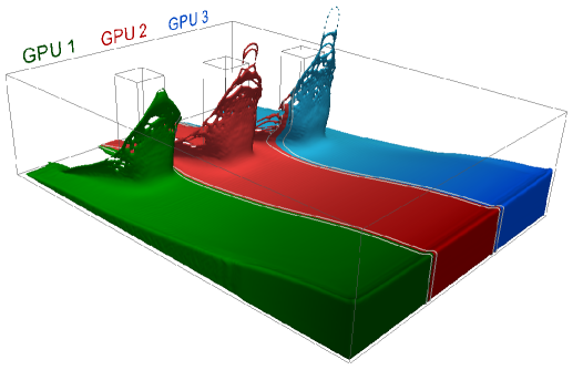
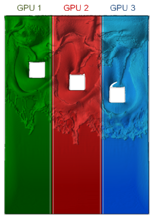
Figure 1: Snapshots of a multi-GPU SPH simulation using three GPUs, for a dam break with three obstacles. Portions of fluid in different sub-domains are displayed with a different color, and white lines near the sub-domain boundaries correspond to the halos.

A second type of acceleration approach is that involving the use of Field-Programmable Gate Arrays (FPGAs). For example, Spurzem et al. [3] carried out SPH and gravitational N-body simulations using this type of technology for astrophysics problems, finding that it is useful for acceleration of complex sequences of operations like those used in SPH. Since the main use of FPGAs in the literature is in the field of astrophysics (where long-range forces and variable smoothing lengths are typically employed), the use of FPGAs for free-surface flow applications (with short-range forces and fixed smoothing lenghts) remains a relatively unexplored field.

The third type of acceleration technique used in SPH simulations, and the one on which this article focuses, involves the use of a type of hardware different from the CPU: the Graphics Processing Unit (GPU). The development of GPU technology is driven by the computer games industry but has recently been exploited for non-graphical calculations, leading to the development of general purpose GPUs (GPGPUs). GPU programming is a parallel approach because each of these devices contains hundreds of computing cores, and multiple threads of execution are launched simultaneously. The use of GPUs for scientific computations has come to represent an exciting alternative for the acceleration of scientific computing software. The release of the Compute Unified Device Architecture (CUDA) and its software development kit (SDK) by NVIDIA in 2007 has facilitated the popularization of the use of these devices for general purposes, but efforts in this direction existed even prior to that date. For example, as early as 2004, Amada et al. [4] carried out SPH simulations for real-time simulations of water. In 2007 Harada et al. [5] reported SPH simulations that ran an order of magnitude faster on GPUs than on CPUs. More recently Hérault et al. [6], reported one to two orders of magnitude speedups of the GPU when compared to a single CPU. Among the recent efforts for SPH computations on GPUs, DualSPHysics [7] has proven to be a versatile computational SPH code for both CPU and GPU calculations. The GPU version of DualSPHysics maintains the stability and accuracy of the CPU version, while providing significant speedups over the latter. For a detailed description of DualSPHysics, please refer to [8].

Recently, in addition to performance, the energy efficiency of different types of hardware is representing an increasingly important factor when choosing hardware for accelerating simulations. This can be seen, for example, in the list of the fastest supercomputers [9], which now include energy efficiency along with performance specifications. In this realm, too, GPUs show promise. For example, a recent article by McIntosh-Smith et al.  [10], describing a methodology for energy efficiency comparisons, reports that in a particular case study of simulations of molecular mechanics-based docking applications, GPUs delivered both better performance and higher energy efficiency than multi-core CPUs.

However, GPU technology has its own constraints. In the particular case of SPH, the memory restricts the maximum number of SPH particles that can be efficiently simulated on a single device to approximately ten million or less, depending on the particular GPU and on the precision of the data types used (e.g., single or double). To go beyond this limit, this work extends DualSPHysics by introducing a spatial decomposition scheme with the use of the Message Passing Interface (MPI) protocolto obtain a multi-GPU SPH application. Thus, our approach combines the two types of parallelization described above since it provides parallelization, first, at a coarse level by decomposing the problem and assigning different volume portions of the system to different GPUs, and second, at a fine level, by assigning one GPU thread of execution to each SPH particle. Our resulting multi-GPU SPH scheme, illustrated in Fig. 1, has the potential to bypass both the system size and simulation time limitations which have to date constrained the applicability of SPH in various engineering fields.

The rest of this article is organized as follows: Section 2 presents a brief overview of the main ideas behind SPH. In Section 3 the methodology used to implement the single-GPU version [8] (which is the starting point for the present work) is summarized. Section 4 describes our spatial decomposition, multi-GPU algorithm, whereby the physical system is divided into sub-domains, each of which is assigned to a different GPU. Section 5 describes the hardware. Section 6 presents the main results of our simulations using a small number of GPUs, including a study of weak and strong scaling, the bottlenecks of the program, and our strategy to diminish the effect of those bottlenecks and improve efficiency. Section 7 concludes with a summary and a description of ongoing and future work.

2 Smoothed Particle Hydrodynamics

In order to better understand the specific challenges posed by a multi-GPU implementation of Smoothed Particle Hydrodynamics (SPH), a brief description of this method is now presented. SPH is a mesh-free, Lagrangian technique particularly well suited to study problems that involve highly non-linear deformation of fluid surfaces that occur in free-surface flows, such as wave breaking and marine hydrodynamics [11]. Developed originally for the study of astrophysical phenomena, it now enjoys popularity in a variety of engineering fields, such as civil engineering (e.g., the design of coastal defenses), mechanical engineering (e.g., impact fracture in solid mechanics studies), and metallurgy (e.g., mould filling).

The problem in SPH consists of determining the evolution in time of the properties of a set of particles representing the fluid. In engineering applications, particles have short range interactions with their neighbours, and the dynamics are governed by a set of simultaneous ordinary differential equations in time. In this section the classical SPH formulation used in our simulations are described (see  [12]).

2.1 Governing equations

The starting point for the derivation of the SPH equations is the set of equations for the continnum description of dynamic fluid flow, namely, the Navier-Stokes equations [13]:

$$\frac{D\rho}{Dt}=-\rho\nabla\cdotp\vec{v},$$ (1)

$$\frac{D\vec{v}}{Dt}=-\frac{1}{\rho}\nabla p+\vec{g},$$ (2)

$$\frac{De}{Dt}=-\frac{p}{\rho}\nabla\cdotp\vec{v}.$$ (3)

Here, $\rho$ is the density, $t$ is time, $\vec{v}$ and $\vec{r}$ represent velocity and position, respectively, $\sigma$ is the total stress tensor, $e$ is the energy, $\vec{g}$ is the force due to gravity, and $D/Dt$ represents the material or total time derivative.

2.2 SPH discretization of the Navier-Stokes equations

Two key steps are used to discretize the Navier-Stokes equations: first, the integral representation of a field function, or kernel approximation, and second, the particle approximation. The value of a field function $f(\vec{r})$ at point $\vec{r}$ can be approximated by a weighted interpolation over the neighbouring volume in the following way:

$$f(\vec{r})\simeq\int_{\Omega}f(\vec{r}^{\prime})W(\vec{r}-\vec{r}^{\prime},h)d\vec{r}^{\prime},$$ (4)

where $W(\vec{r}-\vec{r}^{\prime},h)$ is a smoothing function (also called the smoothing kernel), $h$ is the smoothing length (used to characterize the shape and range of $W$), and the integral is over all space $\Omega$.

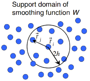
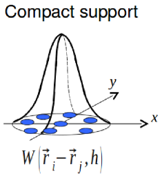
Figure 2: Illustration of the smoothing function, $W(\vec{r}_{i}-\vec{r}_{j},h)$, with a support domain of size $2h$. The blue circles are the particles that represent the fluid. Particle $i$ interact with particle $j$ only if $|\vec{r}_{i}-\vec{r}_{j}|<2h$, due to the compact support property of the smoothing function, as explained in the text.

The smoothing function is typically chosen to have the following properties: its integral over all space is unity; it approaches the Dirac delta function as $h\rightarrow 0$; it has compact support, i.e., its value is zero beyond its support domain $|\vec{r}-\vec{r}^{\prime}|>\kappa h$, where $\kappa$ is a scaling factor used to set the coarseness of the discretization of space (throughout this article $\kappa=2$); it monotonically decreases as $|\vec{r}-\vec{r}^{\prime}|$ increases; and, last, it is symmetric $W(\vec{r}-\vec{r}^{\prime},h)=W(|\vec{r}-\vec{r}^{\prime}|,h)$. It can be shown that the kernel approximation is accurate to order two in $h$, $\mathcal{O}(h^{2})$[14]. In this article, all of the results are obtained using the cubic spline smoothing function [13] with a constantsupport domain of size $2h$.

The second step for the discretization of the Navier-Stokes equations is the particle approximation, which consists simply of replacing the continuous integral in Eq. (4) by a discrete sum, and writing the differential of volume as a finite volume $\Delta V_{j}$ in terms of density and mass, obtaining

$$f(\vec{r}_{i})\simeq\sum_{j}f(\vec{r}_{j})W(\vec{r}_{i}-\vec{r}_{j},h)\frac{m_{j}}{\rho_{j}}$$ (5)

where $m_{j}=\Delta V_{j}\rho_{j}$ is the mass of the SPH particle, and the sum is performed over all neighboring particles in the support domain of $W$.

Figure 2 illustrates some of the properties of the smoothing function $W(\vec{r}_{i}-\vec{r}_{j},h)$. Part (a) of this figure shows particle $i$ interacting with all other particles, $j$, within its radius of influence, or support domain, whereas part (b) shows the compact support in operation, the smoothness of the function, as well as its monotonically decreasing behaviour for increasing $|\vec{r}_{i}-\vec{r}_{j}|$.

Following a similar argument, the particle approximation for the spatial derivative of a function can be written in the following form:

$$\nabla f(\vec{r}_{i})\simeq\sum_{j}[f(\vec{r}_{j})-f(\vec{r}_{i})]\nabla_{i}W(\vec{r}_{i}-\vec{r}_{j},h)\frac{m_{j}}{\rho_{j}}$$ (6)

Mathematically, therefore, the problem consists of performing localised interpolations or summations around each computation point where the properties of the fluid are evaluated.

In the present article, variations in the thermal properties of the fluid are neglected, governed by Eqn. (3), as the primary application of our approach is free-surface flows where thermal properties do not play a significant role. Applying the SPH formulation to the governing equations (1-2) leads to the following set of equations [13]:

$$\frac{d\rho_{i}(t)}{dt} = \sum_{j}m_{j}\vec{v}_{ij}\cdotp\nabla_{i}W_{ij}$$ (7)

$$\frac{d\vec{r}_{i}(t)}{dt} = \vec{v}_{i}(t)$$ (8)

$$\frac{d\vec{v}_{i}(t)}{dt} = -\sum_{j}m_{j}\left(\frac{p_{i}}{\rho_{i}}+\frac{p_{j}}{\rho_{j}}+\Pi_{ij}\right)\nabla_{i}W_{ij}+\vec{g}$$ (9)

where $W_{ij}\equiv W(\vec{r}-\vec{r}_{j},h)$, $\vec{g}$ is gravity, and the artificial viscosity is given by $\Pi_{ij}=\frac{-\alpha\overline{c}_{ij}\nu_{ij}}{\rho_{ij}}\,\text{ if }\vec{r}_{ij}\cdotp\vec{v}_{ij}<0$ and $\Pi_{ij}=0$ otherwise, where $\nu_{ij}=h\vec{v}_{ij}\cdotp\vec{r}_{ij}/(\vec{r}_{ij}^{2}+\eta^{2})$, $\vec{r}_{ij}\equiv\vec{r}_{i}-\vec{r}_{j}$, $\vec{v}_{ij}\equiv\vec{v}_{i}-\vec{v}_{j}$, $\overline{c}_{ij}\equiv(c_{i}+c_{j})/2$, $\eta=0.1h$, $\alpha$ is a parameter that can be related to the Reynolds number for the specific free-surface problem, and $p_{i}$ is the pressure at $r_{i}$, which is governed by the equation of state $p_{i}=B[(\rho_{i}/\rho_{0})^{\gamma}-1]$. Here, $\gamma=7$, $B=c_{0}^{2}\rho_{0}/\gamma$, $\rho_{0}=1000$ Kg/m³, and $c_{0}=\sqrt{(dp/d\rho)|_{\rho_{0}}}$.

2.3 Boundary conditions

In this article dynamic boundary conditions [16] are used to represent solid boundaries. In this method, boundary particles obey the same dynamical equations as the fluid particles, but the integration update for position and velocity is not performed. Therefore, the density and pressure of the particle varies, but the position and veolicty remain fixed (or change in an externally imposed fashion in cases where solid boundaries are moving.)

3 Single-GPU implementation

To describe our multi-GPU implementation, it is useful to review the main strategy behind the single-GPU version, as well as other general considerations that need to be taken into account when performing SPH simulations. For a more detailed description of the single-GPU version of DualSPHysics please refer to [7] and [8].

Single-GPU DualSPHysics is a fully-on-GPU program, meaning that all the calculations, to be described in detail below, are performed on the GPU, and data resides on the GPU memory at all times, and is copied to the host only when saving of the simulation results is required. In this way the time consuming transfers of data between CPU and GPU are minimized. This fully-on-GPU strategy contrasts with other approaches which only partially port computations to the GPU [17].

Some, but not all, of the tasks involved in the GPU implementation of an SPH simulation are easily parallelized. The difficulties mainly arise from the Lagrangian nature of the method, where particles move in space. The following basic strategies were followed to increase performance: minimization of GPU-CPU data transfers; optimization of memory usage to increase bandwidth; minimization of divergent warps; optimization of memory access patterns; and maximization of occupancy to hide latency.

An SPH simulation consists of solving the set of equations (7)-(9) at discrete points in time. To achieve this, a series of iterations is performed:

1. Find the neighbours of each particle, that is, all other particles within its support domain of $2h$

2. Sum the pairwise interactions between each particle and its neighbours

3. Update the system with the use of an integrator

We now describe the GPU implementation of those steps.

3.1 Finding particle neighbours

To determine the neighbours of each particle efficiently, the domain space is divided into cubic cells of the size of the kernel support domain, namely $2h$. Then a CUDA kernel is launched, with one thread per particle, that assigns to each particle a label corresponding to the cell to which it belongs. The next step consists of using the radix sort algorithm [18] to order the array holding the particle identification labels, or IDs, according to the cell to which the particle belongs. Next all arrays containing data information (position, velocity, etc.) are ordered according to the newly ordered ID array. Last, an extra array is generated with the index of the first particle of each cell that enables neighbour identification during the computation of the particle interactions.

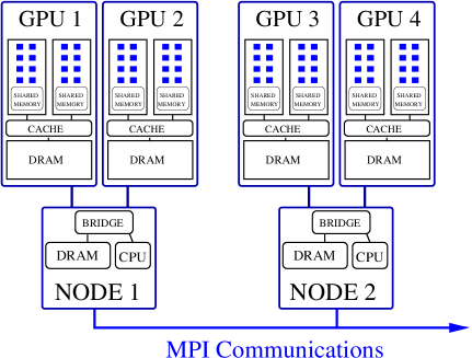
Figure 3: Illustration of a multi-GPU system with two nodes, each hosting two GPUs. More generally, a multi-GPU system consists of one or more computing nodes, each hosting one or more GPUs, in addition to one or more CPUs. Different nodes are connected via a computer networking technology, and transfer of information is performed with MPI.

3.2 Computing particle interactions

With the arrays re-ordered according to cells, and the index of the first particle of each cell, a new CUDA kernel is launched. One CUDA thread is assigned to each particle $i$ to search for its neighbours. If particle $i$ is in cell $c$, the thread will look for neighbours only in cell $c$ and in cells adjacent to $c$. This CUDA thread will also compute the interaction between particle $i$ and its neighbours, that is, the sum on the right-hand side of equations (7)-(9).

3.3 System update

Once the interactions are computed, and the right-hand side of equations (7)-(9) is known, the system state can be updated by numerical integration. As with any other set of simultaneous first-order ordinarly differential equations, a variety of integration schemes can be used [19], and here a second-order Verlet algorithm is used. The size of the integration time step varies throughout each simulation according to the Courant-Friedrichs-Lewy (CFL) condition [20] and the magnitude of the interactions. Here, minimum and maximum values of certain physical quantities need to be found among all particles, and for this, efficient CUDA reduction algorithms provided by NVIDIA are employed.

3.4 Single-GPU versus single-CPU approaches

Previous work concerning HPC for SPH published prior to the appearance of GPUs report results using either small CPU clusters or large supercomputers, such as Blue-Gene. It is generally misleading to compare the performance of a specific number of GPU cores to a CPU core as the architecture and potential performance is quite different. However, when demonstrating the advantages of GPU computations for engineering applications within industry, the ability to contrast the relative runtimes can be both accessible and useful. Hence, results can be expressed in terms of speedup and efficiency by comparing the number of cores versus a single core. Therefore, to analyse the performance of one GPU, the speedup in comparison with a single CPU core is also shown to give an idea of the order of speedup that is possible when using low-cost and accessible GPU cards, instead of large cluster machines.

We have observed (see Ref. [8]) that the GPU version of DualSPHysics runs on the order of 60 times faster than its single-threaded CPU version. For this comparison, an NVIDIA GTX480 GPU and an Intel Core i7 were used. In the CPU code, all of the standard CPU optimizations were applied, symmetry in particle-particle interaction was employed, and SIMD instructions that allow performing operations on data sets were used whenever possible. However, if a multi-threaded, OpenMP approach is used on a multi-core CPU instead (4 cores of a CPU Intel Core i7, with 8 logical cores using Hyperthreading) the speedup of the GPU over the CPU was 14. In this way, for the mentioned hardware one can estimate a speedup of approximately $60/nc$ where $nc$ is the number of CPU cores used.

4 Multi-GPU implementation

As mentioned in Section 3, single-GPU DualSPHysics has proved to be a viable option for accelerated SPH simulations. However, for a fully-on-GPU approach as presented here, there is a limitation on the number of particles that can be simulated due to the size of the GPU memory. For example, a commonly used NVIDIA GPU, the GTX480, with 1.5 GB of memory, can handle up to about 8 million SPH particles, and an NVIDIA Tesla M2050 can simulate a maximum of about 15 million particles. To go beyond the limitsimposed by those constraints, a spatial decomposition scheme is introduced (illustrated in Fig. 1) with the use of MPI to communicate between different GPUs, which is explained in this section.

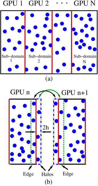
Figure 4: (a) One-dimensional domain decomposition scheme for a computational system with $N$ GPUs. The total physical volume is divided into $N$ sub-domains, each of which is assigned to a different GPU. Data needs to transferred between GPUs when there is flow from one sub-domain to another, and also when the halo needs to be updated. (b) Data needed to process the dynamics of particles within the range of interaction (a distance of twice the smoothing length, $2h$, in our case) is stored in the halo of the sub-domain.

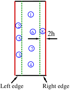
Figure 5: The “edges” of a sub-volume are used to construct the halo of neighbouring sub-domains. The illustrated sub-domain is assumed to have neighbouring sub-domains both to the left and to the right, and therefore data arrays containing particle state are ordered with the use of radix sort routine, as explained in detail in the text.

4.1 A multi-GPU system

To understand the computational tasks required for a multi-GPU SPH simulation, we begin with a brief description of our multi-GPU system. Fig. 3 shows a schematic view of one such system, consisting of two computing nodes, each hosting one CPU and two GPUs. More generally, a multi-GPU system consists of one or more computing nodes, each hosting one or more GPUs, in addition to one or more CPUs. Nodes are connected with each other via a computer networking technology, and the transfer of data between nodes is executed using a protocol, in this case MPI, whereas each GPU is connected to its host via a PCI Express bus. Throughout the rest of this article, the words “CPU”, “node” and “host” are used interchangeably.

4.2 Spatial decomposition

The main idea behind the implementation of our scheme is to assign different parts of the physical system to different GPUs—that is, a volume domain decomposition technique is used. The portion assigned to a GPU is referred to as a “sub-domain” throughout the rest of this article. Eventually, the intention is to use a multi-dimensional domain decomposition with load balancing. For the development of the algorithm presented herein, a one-dimensional decomposition is sufficient. Fig. 1 illustrates a domain decomposition scheme in operation for a three-dimensional dam break simulation with three obstacles. During and after each integration step, data needs to be transferred between GPUs due to, firstly, particles migrating from one sub-domain to another, and secondly, information of particles residing on a neighbour sub-domain that are close enough to the boundary to influence the dynamics of particles in the domain of interest, that is, the ’halo building’ process. This requires three main steps: preparation of the data, as well as GPU-CPU communications, and inter-CPU communications. Preparation of data is the process by which a GPU re-arranges the information to be passed to other GPUs before actually sending it. An example of this is the re-ordering of the arrays containing the state of particles when they step out of their sub-domain, so that the relevant information is efficiently packaged before it is copied to the CPU (host) memory.

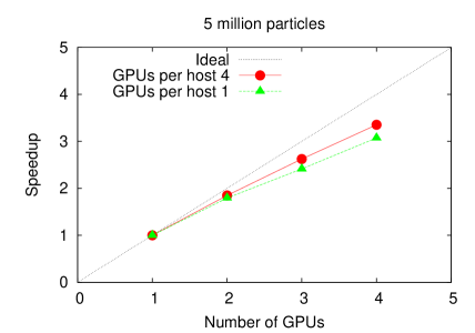
Figure 6: Strong scaling behaviour for the speedup of a dam break simulation with 5 million particles. The red curve corresponds to simulations run on the system with up to four GPUs, all residing on the same node, whereas the green curve shows results using one GPU per node.

Fig. 4a illustrates a one-dimensional domain decomposition scheme for a computational system with $N$ GPUs. The total physical volume is divided accordingly into $N$ sub-domains (boundaries are shown in red in Fig. 4), each of which is assigned to a different GPU. Fig. 4b shows two neighbouring domains, $n$, and $n+1$. Data from the edge (the portion of the sub-domain within a distance $2h$ to the sub-domain boundary) of domain $n$ is used to construct the halo of the neighbouring domain $n+1$, and vice versa. The width of the halo and the width of the edge are the size of the interaction range, in our case, twice the smoothing length, $2h$.

For the sake of clarity, in the rest of this sub-section we assume a muti-GPU system with $N$ nodes. Each node is labelled with the number $k$ (with $k=1,2,\ldots N$) and hosts only one CPU (CPU_k) and one GPU (GPU_k). There is, then, one MPI process, $p_{k}$, per GPU, and $p_{k}$ controls GPU_k, which is assigned to sub-domain $S_{k}$. After $p_{k}$ sets the initial state $Q_{k}$ (position, velocity, etc.) of particles in $S_{k}$ and its halo $H_{k}$, the program iterates over the following steps:

• Determine integration step size, $\Delta t$

• GPU_k: update state, $Q_{k}$

• GPU_k: if any particles now have positions corresponding to a different sub-domain $S_{j}$, with $j\neq k$, then

  • GPU_k: label particles according to sub-domain

  • GPU_k: order arrays according to sub-domain label (using radix sort)

  • GPU_k: copy data, $D_{send}$, from GPU_k to CPU_k, of particles migrating from one sub-domain to another

  • CPU_k: send $D_{send}$ to $p_{j}$, with $j\neq k$

  • CPU_k: receive data, $D_{receive}$, from $p_{j}$, with $j\neq k$

  • GPU_k: copy $D_{receive}$ from CPU_k to GPU_k

  • GPU_k: update number of particles in sub-domain $k$

• if saving data, then

  • GPU_k: copy data of all particles in sub-domain from GPU_k to CPU_k

• GPU_k: label particles according to edge

• GPU_k: order arrays according to edge label (using radix sort)

• GPU_k: copy data, $E_{send}$, of edge particles, from GPU_k to CPU_k

• CPU_k: send $E_{send}$ to $p_{j}$, with $j\neq k$

• CPU_k: receive data, $E_{receive}$, from $p_{j}$, with $j\neq k$

• GPU_k: copy $E_{receive}$ from CPU_k to GPU_k

• GPU_k: update number of particles in sub-domain $k$

• GPU_k: order arrays according to cubic cell of size $2h$

Determining the size of $\Delta t$, which is the same for all sub-domains, involves two kinds of reduction operations: one on the GPU, where each device GPU_k determines the minimum size of $\Delta t_{k}$ suitable for the numerical integration for particles in its sub-domain, and then another, on the CPUs, whereby the minimum among all $\Delta t_{k}$’s is found with an MPI Allreduce operation.

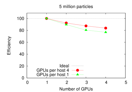
Figure 7: Efficiency for the simulations described in Fig. 6.

In summary, the multi-GPU program iterates over the next three main steps:

1. Update particle state: Each GPU updates the state of the particles within the sub-domain assigned to it. This involves (i) re-ordering data arrays that hold the state of the particles to determine efficiently their neighbours (using the radix sort algorithm), (ii) computing the inter-particle interactions (e.g., the forces), and (iii) the actual update of the particle state.

2. Update sub-domains: the number of particles in each sub-domain must be updated to reflect particle migration due to fluid flow, and the state of migrated particles must be transferred accordingly. This is achieved by re-ordering data arrays (using the radix sort algorithm) according to the sub-domain in which they are located, and then transferring the necessary data from the GPU to the CPU, then among CPUs if the GPUs reside on different hosts, and last, from the CPU to the new GPU.

3. Update sub-domain halo: The halo holds the data of particles that exist on a neighbouring sub-domain but close enough to influence the particles of the domain in question (a distance twice the smoothing length $h$ in our case, see Fig. 4b). Here again the radix sort algorithm is used to re-order data arrays according to the halo to which they they may belong.

In its current version, the scheme does not include task overlapping of computation on each GPU with communications among those devices. Since the computation of the particles inside a given sub-domain requires an up-to-date state of the particles within its halo, it is not possible for a given GPU to send data to another device before the computation is finished, which prevents the overlap of computation and communication.

In regards to overlapping of CPU and GPU computation, the highly parallelizable nature of the SPH algorithm, in conjunction with the high cost of GPU-CPU communications, makes fully-on-GPU schemes more efficient, at least in single-GPU computations. This has been discussed in Ref. [17] (e.g., see Figure 1 of that work). However, it is conceivable that in multi-GPU approaches, due to the fact that data needs to be transferred among GPUs via the CPU, one could perform some of the computations on the CPU, thereby saving GPU-to-CPU communication time. This idea remains to be explored.

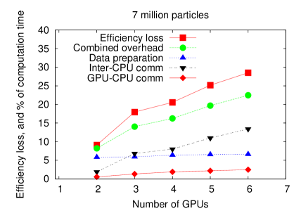
Figure 8: Efficiency loss is compared to the percentage of time consumed by various computational tasks in a multi-GPU simulation.

4.3 Using the radix sort algorithm

To illustrate the use of the radix sort algorithm for the halo updating procedure, we use Fig. 5. It is assumed that the sub-domain represented in this figure has neighbour sub-domains both to the left and to the right. Particles labelled 2, 5, and 3 are within a distance $2h$ from the sub-domain boundary to the left and therefore form the left “edge”, whereas particle labelled $8$ is within this distance to the sub-domain boundary to the right, and forms the right “edge”. Particles 1, 4, 6, and 7 are further than $2h$ from either boundary and therefore do not belong to any edge. When the update of the halo of the sub-domain neighbouring to the left is made, the state of particles on the left edge needs to be passed to the GPU assigned to it. To achieve this, first a CUDA kernel is launched which assigns to particles not in a halo the label “0”, and to particles on the left halo a label “1”, and to particles in the right halo the label “2”:

$$halo = \{{\color[rgb]{1,0,0}0,\,1,\,1,\,0,\,1,\,0,\,0,\,2}\},$$

$$id = \{{\color[rgb]{0,0,1}1,\,2,\,3,\,4,\,5,\,6,\,7,\,8}\},$$

where “halo” and “id” are one-dimensional data arrays of integers, containing the assigned label, and the particle identification number, respectively.

Next the radix sort routine is called to obtain a re-ordered array of the particles identification numbers, according to the “halo” label:

$$halo = \{{\color[rgb]{1,0,0}0,\,0,\,0,\,0,\,1,\,1,\,1,\,2}\},$$

$$id = \{{\color[rgb]{0,0,1}1,\,4,\,6,\,7,\,2,\,3,\,5,\,8}\}.$$

The new version of the array ID is used to re-order all of the arrays containing the state of the particles, namely, the one dimensional array for positions, velocities, etc. Once this reordering is made, the CUDA function cudaMemcpy is used to transfer the relevant data from the GPU to the CPU, and, if the GPUs reside on different hosts, then an inter-node communication is made before uploading the data in question onto the desired GPU.

A similar procedure to the construction of the halo is used for the data transfers due to particle migration. In this case, particles are assigned labels depending on the sub-domain to which they have migrated: “1” if they migrated to left, “2” if they migrated to the right, and “0” otherwise, and data is transferred accordingly after reordering the data arrays containing the particle state, similar to the construction of the halo.

4.4 Other approaches to multi-GPU programming

There are three main features which make our scheme different to other multi-GPU approaches for SPH (for example, [17]):

1. the use a low-level CUDA approach instead of a high-level, directive-based transformation of CPU to GPU code;

2. the full implementation of the computations on the GPU, instead of porting to the GPU only part of the computations, and performing the rest on the CPU; and

3. the fact that the code development starts from a single-GPU code and progresses towards a multi-GPU application, instead of going from a multi-CPU to a multi-GPU program.

The use of a low-level approach, combined with the fact that the computation is fully implemented on the GPU [points (1) and (2)], facilitates a higher level of control of the hardware, the utilization of the memory hierarchies, as well as the use of highly optimized CUDA functions. These features are not as readily available in directive-based approaches. Additionally —and in regards to multi-GPU programming— the advantage of these two features is the straightforward availability of both data and optimized CUDA sub-routines to process it, for instance, during the construction of the halo and the migration of particles, which are crucial steps in the scheme.

The advantage of point (3) is related to the previous two points, where the data structures and tools for the multi-GPU scheme were present and thoroughly tested on the single-GPU version before making the extension to multi-GPU. For instance, the routines for sorting and determining the labels of the first and last particle in a given region of space were already used in single-GPU method for finding neighbours of particles, and when implementing the multi-GPU version they were re-used for determining migrating particles as well as the edges and halos in a sub-domain, as explained in detail above.

5 Hardware

Simulations have been performed on two different systems: one is part of a dedicated cluster at the University of Manchester, where the GPU section has six nodes each hosting two NVIDIA Tesla M2050, which feature the Fermi architecture, and each possess 448 computing cores grouped in 14 streaming multiprocessors of 32 cores each, clock rate of 1.15 GHz, 3 GB GDDR5 memory, and a high speed, PCI-Express bus, Gen 2.0 Data Transfer. The hosting nodes are connected via 1 Gigabit per second Ethernet technology, which, unfortunately, is much slower than Infiniband, with its current speed of 40 Gigabits per second and significantly lower latency, to which we currently have no access. Each of the hosting nodes also has two six-core AMD Opteron processors (CPUs), and runs Scientific Linux release 5.5.

The second system used for simulations is a single node hosting four GPUs at the University of Vigo, Spain. The GPUs are NVIDIA GTX480, which, like the M2050, feature a Fermi architecture and 448 computing cores, but have a faster clock rate of 1.4 GHz, and a smaller memory of 1.5 GB GDDR5. The connection to the host is done via a PCI-Express bus. Additionally, the hosting node has two Intel Xeon E5620 2.4 GHz CPUs, and since all four GPUs reside on the same host, there is no need for a computer networking technology.

6 Results

To test our multi-GPU program, simulations of a three-dimensional dam break with three obstacles, illustrated in Fig. 1 were performed. When assessing parallelization, it is useful to address questions of efficiency and scalability in order to determine the usefulness of the approach used. The aim of this section is to answer the following questions:

• Scaling: how do computing times change when the system size and the number of computing devices (in our case, the number of GPUs) vary?

• Where are the bottlenecks? Are they in the GPU to CPU or in inter-CPU data transfers? Or are they on the data preparation routines?

• How does the overhead resulting from data transfers between GPUs (due to particle migration and halo construction) compare to the time spent by each GPU processing the motion of particles in its assigned sub-domain?

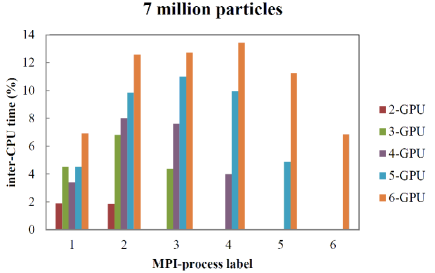
Figure 9: Percentage of time that each MPI process uses for inter-CPU communications for simulations using different number of GPUs. The horizontal axis corresponds to the label of the MPI process. Smaller times correspond to the processes assigned to endpoints of the simulation box, as explained in more detail in the text.

The speedup $s$ of the multi-GPU simulations is defined as a function of the number of GPUs $N$ in the following way:

$$s(N)=\frac{T(N_{\textsc{ref}})n_{p}(N)}{T(N)n_{p}(N_{\textsc{ref}})}$$ (10)

where $T$ is the simulation time divided by the number of steps $N_{steps}$, $N_{\textsc{ref}}$ is the number of GPUs used as reference (in this article, $N_{\textsc{ref}}=1$), and $n_{p}$ is a measure of the system size, which in this article is the number of particles. The efficiency $\eta$ is defined as the speedup divided by the number of GPUs:

$$\eta(N)=\frac{s(N)}{N}.$$ (11)

Two types of scaling behaviour are investigated, weak and strong, which are now described.

6.1 Strong scaling

Strong scaling is studied by increasing the number of GPUs while leaving the system size (both the number of particles and the physical dimensions) fixed $n_{p}(N)=n_{p}(N_{\textsc{ref}})$. Substituting this in (10) we obtain

$$s(N)=\frac{T(N_{\textsc{ref}})}{T(N)}.$$ (12)

In the ideal case the computation time is inversely proportional to the number of GPUs used, $T(N)=c/N$, where $c$ is the proportionality constant, giving $s(N)=N/N_{\textsc{ref}}$. If the reference number of GPUs $N_{\textsc{ref}}=1$, then $s(N)=N$.

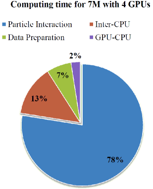
Figure 10: Comparison of the percentage of the computation time spent by different tasks carried out during a 4-GPU simulation of a dam break, using 7 million particles, where each GPU resides on a different computing node.

Fig. 6 shows results for the strong scaling behaviour of our program for the speedup, for a dam break simulation of 5 million particles, on the two systems described in Section 5. 5 million particles was chosen because this number is close to the maximum number of particles that can currently fit into a single NVIDIA GTX480 used for comparisons here. The red curve corresponds to simulations run on the system with up to four GPUs, all residing on the same node, whereas the green curve shows results using one GPU per node. As expected, the speedup is better in the first case, where there is no need for inter-CPU (inter-node) communications. Fig. 7 shows the corresponding results for the efficiency for the system described in Fig. 6.

In Fig. 8, the efficiency loss, defined as $100-\eta$ (where $\eta$ is the efficiency, plotted in Fig. 7), is compared to the percentage of time consumed by various computational tasks in a multi-GPU simulation. From this, it can be observed that (i) a correlation exists between the combined overhead (sum of inter-CPU, GPU-CPU communication and data preparation times, in green circles) and the loss of efficiency (in red squares), and (ii) that the overhead increases with the number of GPUs mostly due to the inter-CPU communications (black triangles), since the overhead caused by GPU-CPU communications (red diamonds) and data preparation (blue triangles) increases much more slowly. Note that, since each MPI process in a given simulation measures its own communication times, and those times are in general different from one process to another, here the longest time among all processes of a given simulation is used. This will be further discussed for Fig. 9 below.

In future versions of our program, the total overhead is expected to be reduced with (a) the use of pinned memory for faster the GPU-CPU data transfers, and (b) the utilization of an Infiniband switch, which should substantially decrease the inter-CPU communications. Also, for the case of GPUs residing on the same host, the introduction of CUDA 4.0 should result in further reduction of overhead. As mentioned earlier, two-dimensional domain decomposition is envisaged, which will entail a significant increase of the inter-CPU communication times, especially on systems that use slow inter-CPU networking technology, such as Gigabit Ethernet, instead of Infiniband or faster versions of Ethernet. The reason for this is that for two-dimensional domain decomposition, each MPI process will need to send information to as many as eight other processes when doing the inter-CPU communications on system with many nodes.

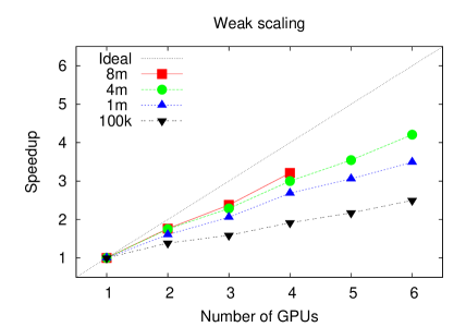
Figure 11: Simulations using a number of particles proportional to the number of GPUs. Plots are shown for $n_{sub}$ (number of particles per GPU) equal 100 thousand, 1, 2, 4, and 8 million.

Figure 9 shows the percentage of time that each MPI process uses for inter-CPU communications for 2-, 3-, 4-, 5-, and 6-GPU simulations. The horizontal axis corresponds to the label of the MPI process. Each label is assigned in order of increasing $y$-coordinate to the ’slices’ into which the simulation box has been subdivided (e.g., Fig. 1 for the particular case of three GPUs). One can see that the time is smaller for the processes assigned to sub-volumes on the edges of the simulation box than for the rest, reflecting the fact that processes on the edge need to send data to one neighbour process only, whereas the rest of them need to send data to two neighbours instead.

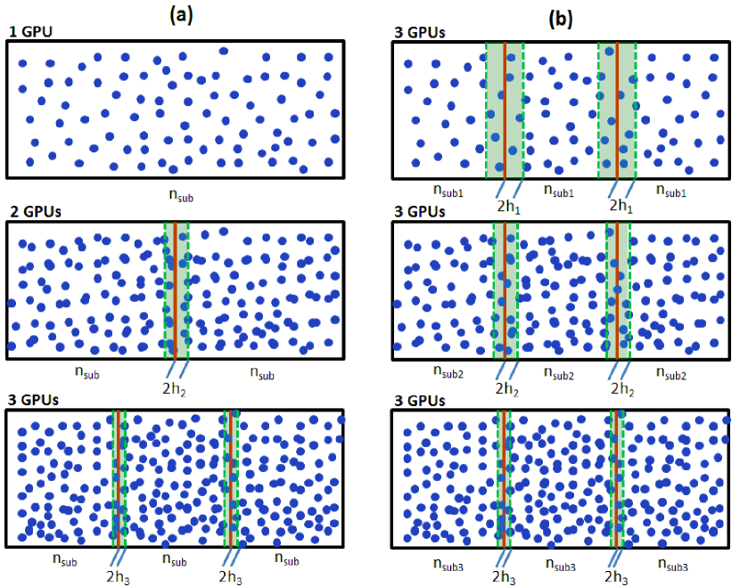
Figure 12: (a) Domain decomposition scheme for a fixed number of particles $n_{sub}$ per GPU, and an increasing number of GPUs, corresponding to weak scaling. (b) For a given number of GPUs (three in this example), one can show that the ratio of particles in the halo $n_{halo}$ to $n_{sub}$ decreases, leading to the better scaling that can be seen in Fig. 11. See text for details.

In Fig. 10 some of the most consuming tasks of a multi-GPU simulation are compared for a dam break with 7 million particles on four GPUs. This figure shows that the time that each GPU uses to compute the particle dynamics (once its halo has been updated) is nearly 80% of the total simulation time, dominating the overall computation. However, considerable time is also spent on inter-CPU communications, and, to a lesser extent, data preparation, and GPU-CPU data transfers.

6.2 Weak scaling

Simulations have also been performed using system sizes proportional to the number of GPUs : $n_{p}(N)=Nc$, where $c$ is the proportionality constant. Substituting this in (10) we get

$$s(N)=\frac{T(N_{\textsc{ref}})N}{T(N)N_{\textsc{ref}}}.$$ (13)

In the ideal case the time is the same regardless of the number of GPUs, $T(N)=T(N_{\textsc{ref}})$ and $s(N)=N/N_{\textsc{ref}}$. If the reference number of GPUs $N_{\textsc{ref}}=1$, then $s(N)=N$.

Fig. 11 shows the results of simulations using a number of particles proportional to the number of GPUs. Plots are shown for 100 thousand, 1, 2, 4, and 8 million particles per GPU, with the largest simulation so far being for 32 million particles distributed among four GPUs. As expected, scaling improves with a growing number of particles per GPU because the time spent on tasks that result in an overhead becomes a smaller percentage of the total computational time, which, as shown in Fig. 10, is dominated by the update of particle states performed by each GPU.

One must note that, for each curve in Fig. 11, the total number of particles in the system is increased by making a finer discretization of the continuum, that is, by using smaller particles (smaller smoothing length $h$), instead of increasing the physical dimensions of the simulation box (here this is kept fixed). In this scenario, one can demonstrate that the larger the number $n_{sub}$ of particles per GPU, the smaller the fraction $n_{halo}/n_{sub}$, which leads to better scaling.

To demonstrate this, consider the ratio

$$\frac{n_{halo}}{n_{sub}}\sim\frac{LH2h}{LHW/N}=\frac{N2h}{W},$$ (14)

where $L$, $H$, and $W$ are the length, height and width of the simulation box, $LH2h$ is the volume of the halo, and $LHW$ is the total domain of the simulation box, which, divided by $N$, gives the volume of the sub-domain. Since the volume of one particle is proportional to $h^{3}$, for a fixed fluid volume the total number of particles in a simulation is given by $n_{p}=Nn_{sub}\sim h^{-3}$. We can therefore write:

$$\frac{n_{halo}}{n_{sub}}\sim\frac{N^{2/3}}{n_{sub}^{1/3}}.$$ (15)

This means that, for a fixed number of GPUs $N$, the number of particles in the halo, relative to the number of particles in the sub-domain, shrinks. This is illustrated in Fig. 12. In part (a), a fixed number of particles per GPU with an increasing number of GPUs is shown, corresponding to weak scaling. One can observe the reduction of the size of the halo, which is of size 2$h$. Part (b) of this figure shows also decreasing halo size as number of particles is increased while keeping the number of GPUs fixed.

6.3 Scaling comparison

It is instructive to compare the scaling results presented in this article with those of other multi-GPU and multi-CPU approaches. Oger et al [17] describe a multi-GPU SPH scheme that uses directive-based, partially-ported GPU code. Although that report does not present the same kind of scaling as we do here, one can extract some useful information from their data. In particular, from their Figure 9, one can obtain an approximation to their strong scaling behaviour by dividing the time their simulation takes on two nodes by the time it takes on four nodes, which in the ideal scaling case would yield 2. In Ref. [17] this value is approximately 1.7 (for 155,500 particles) and 1.8 (for 2,474,000 particles). The same division using our data for five million particles gives approximately 1.7, showing consistency between the two schemes.

A comparison with multi-CPU code is also interesting. For example, Maruzewski et al. [1] report both strong and weak scaling on SPH simulations on as many as 1024 CPU cores, with a number of particles of up to 124 million. As it is often the case in this type of multi-CPU simulations, scaling data (Figures 5, 6, and 7 in Ref. [1]) shows no significant departure from the ideal value until the number of CPUs is relatively large, on the order of eight in this case.

A plausible explanation for the worse scaling behaviour on multi-GPU systems than on multi-CPU clusters has been proposed in Ref. [21] for Molecular Dynamics simulations. In essence, the part of the program computing the motion of particles is accelerated by the GPU, but the inter-device communications are not. Therefore, the time spent on the latter, as a fraction of the total simulation time, becomes relatively large more quickly as the number of computing devices is increased.

7 Summary and future work

This paper presented a computational methodology to carry out three-dimensional, massively parallel Smoothed Particle Hydrodynamics (SPH) simulations across multiple GPUs. This has been achieved by introducing a spatial domain decomposition scheme into the single-GPU part of the DualSPHysics code, converting it into a multi-GPU SPH program.

By using multiple GPUs, on the one hand, simulations can be performed that could also be performed on a single GPU, but can now be obtained even faster than on one of these devices alone, leading to speedups of several hundred in comparison to a single-threaded CPU program. On the other hand accelerated simulations with tens of millions of particles can now be performed, which would be impossible to fit on a single GPU due to memory constraints in a full-on-GPU simulation where all data resides on the GPU. By being able to simulate—without the need of large, expensive clusters of CPUs—this large number of particles at speeds well beyond one hundred times faster than single CPU programs, our software has the potential to bypass limitations of system size and simulation times which have been constraining the applicability of SPH to various engineering problems.

The methodology features the use of MPI routines and the sorting algorithm radix sort, for the migration of particles between GPUs as well as domain ’halo’ building. A study of weak and strong scaling with a slow Ethernet connection shows that inter-CPU communications are likely to be the bottleneck of our simulations, but considerable overhead is also produced by data preparation, and, to a lesser extent, by GPU-CPU data transfers. A possible solution to the overhead caused by the latter is the use of pinned memory, which so far in our program remains unused. The use of Infiniband instead of Ethernet should reduce the overhead cause by inter-CPU communications, and for the case of GPUs residing on the same host, the use of the recently released CUDA 4.0 will be introduced, which should further accelerate communications. Future work includes also the introduction of a dynamic load balancing algorithm, a multi-dimensional domain decomposition scheme, as well as floating body capabilities.

References

- [1] P. Maruzewski, D. Le Touzé, G. Oger, F. Avellan, SPH High-Performance Computing simulations of rigid solids impacting the free-surface of water, Journal of Hydraulic Research 48 (Extra Issue (2010)) (2010) 126–134. doi:10.3826/jhr.2009.0011.
- [2] A. Ferrari, M. Dumbser, E. F. Toro, A. Armanini, A new 3d parallel sph scheme for free surface flows, Computers and Fluids 38 (6) (2009) 1203 – 1217. doi:DOI:10.1016/j.compfluid.2008.11.012.
- [3] R. Spurzem, P. Berczik, G. Marcus, A. Kugel, G. Lienhart, I. Berentzen, R. Männer, R. Klessen, R. Banerjee, Accelerating astrophysical particle simulations with programmable hardware (FPGA and GPU), Computer Science Research and Development 23 (3-4) (2009) 231–239.
- [4] T. Amada, M. Imura, Y. Yasumuro, Y. Manabe, K. Chihara, Particle-based fluid simulation on GPU, in: ACM Workshop on General-Purpose Computing on Graphics Processors and SIGGRAPH, 2004.
- [5] T. Harada, S. Koshizuka, Y. Kawaguchi, Smoothed particle hydrodynamics on GPUs, Proceedings of Computer Graphics International (2007).
- [6] A. Hérault, G. Bilotta, R. A. Dalrymple, SPH on GPU with CUDA, Journal of Hydraulic Research 48 (1 supp 1) (2010) 0022–1686. doi:10.1080/00221686.2010.9641247.
- [7] http://dual.sphysics.org.
- [8] A. J. C. Crespo, J. Domínguez, A. Barreiro, M. Gómez-Gesteira, B. D. Rogers, GPUs, a new tool of acceleration in cfd: Efficiency and reliability on smoothed particle hydrodynamics methods, PLoS ONEdoi:doi:10.1371/journal.pone.002068.
- [9] http://www.top500.org/.
- [10] S. McIntosh-Smith, T. Wilson, J. Crisp, A. A. Ibarra, R. B. Sessions, Energy-aware metrics for benchmarking heterogeneous systems, SIGMETRICS Perform. Eval. Rev. 38 (2011) 88–94.
- [11] J. C. Campbell, R. Vignjevic, M. Patel, S. Milisavljevic, Simulation of Water Loading On Deformable Structures Using SPH, CMES-COMPUTER MODELING IN ENGINEERING & SCIENCES 49 (1) (2009) 1–21.
- [12] M. Gómez-Gesteira, B. D. Rogers, R. A. Dalrymple, A. Crespo, State-of-the-art of classical sph for free-surface flows, Journal of Hydraulic Research 48 (2010) 6–27.
- [13] G. Liu, M.B.Liu, Smoothed Particle Hydrodynamics, a meshfree particle method, World Scientific, 2003.
- [14] J. J. Monaghan, Why particle methods work, SIAM Journal on scientific and statistical computing 3 (1982) 422–433.
- [15] D. M. Acreman, T. J. Harries, D. A. Rundle, Modelling circumstellar discs with three-dimensional radiation hydrodynamics, Monthly Notices of the Royal Astronomical Society 403 (2010) 1143–1155. arXiv:0912.2030.
- [16] A. Crespo, M. Gómez-Gesteira, R. A. Dalrymple, Boundary conditions generated by dynamic particles in sph methods, Computers, materials and continua 5(3) (2007) 173–184.
- [17] G.Oger, E. Jacquin, M. Doring, P.-M. Guilcher, R. Dolbeau, P.-L. Cabelguen, L. Bertaux, D. L. Touzé, B. Alessandrini, Hybrid CPU-GPU acceleration of the 3-D parallel code sph-flow, in: Proc 5th International SPHERIC Workshop, Ed. B.D. Rogers, 2010, pp. 394–400.
- [18] N. Satish, M. Harris, M. Garland, Designing efficient sorting algorithms for manycore GPUs, in: Proceedings of IEEE International Parallel and Distributed Processing Symposium 2009, 2009.
- [19] W. H. Press, S. A. Teukolsky, W. T. Vetterling, B. P. Flannery, Numerical recipes in C (2nd ed.): the art of scientific computing, Cambridge University Press, New York, NY, USA, 1992.
- [20] M. Gómez-Gesteirra, B. D. Rogers, R. A. Dalrymple, A. Crespo, M. Narayanaswamy, SPHysics - development of a free-surface fluid solver- Part 1: Theory and Formulations, Computers and Geosciences, doi:10.1016/j.cageo.2012.02.029 .
- [21] C. R. Trott, L. Winterfeld, P. S. Crozier, General-Purpose molecular dynamics simulations on GPU-based clusters (2011). arXiv:1009.4330v2 [cond-mat.mtrl-sci].