Improved Quantum Query Algorithms for
Triangle Finding and Associativity Testing

Abstract

We show that the quantum query complexity of detecting if an $n$-vertex graph contains a triangle is $O(n^{9/7})$. This improves the previous best algorithm of Belovs [2] making $O(n^{35/27})$ queries. For the problem of determining if an operation $\circ:S\times S\rightarrow S$ is associative, we give an algorithm making $O(|S|^{10/7})$ queries, the first improvement to the trivial $O(|S|^{3/2})$ application of Grover search.

Our algorithms are designed using the learning graph framework of Belovs. We give a family of algorithms for detecting constant-sized subgraphs, which can possibly be directed and colored. These algorithms are designed in a simple high-level language; our main theorem shows how this high-level language can be compiled as a learning graph and gives the resulting complexity.

The key idea to our improvements is to allow more freedom in the parameters of the database kept by the algorithm. As in our previous work [9], the edge slots maintained in the database are specified by a graph whose edges are the union of regular bipartite graphs, the overall structure of which mimics that of the graph of the certificate. By allowing these bipartite graphs to be unbalanced and of variable degree we obtain better algorithms.

1 Introduction

Quantum query complexity is a black-box model of quantum computation, where the resource measured is the number of queries to the input needed to compute a function. This model captures the great algorithmic successes of quantum computing like the search algorithm of Grover [5] and the period finding subroutine of Shor’s factoring algorithm [12], while at the same time is simple enough that one can often show tight lower bounds.

Recently, there have been very exciting developments in quantum query complexity. Reichardt [11] showed that the general adversary bound, formerly just a lower bound technique for quantum query complexity [7], is also an upper bound. This characterization opens a new avenue for designing quantum query algorithms. The general adversary bound can be written as a relatively simple semidefinite program, thus by providing a feasible solution to the minimization form of this program one can upper bound quantum query complexity.

This plan turns out to be quite difficult to implement as the minimization form of the adversary bound has exponentially many constraints. Even for simple functions it can be challenging to directly write down a feasible solution, much less worry about finding a solution with good objective value.

To surmount this problem, Belovs [2] introduced the beautiful model of learning graphs, which can be viewed as the minimization form of the general adversary bound with additional structure imposed on the form of the solution. This additional structure makes learning graphs easier to reason about by ensuring that the constraints are automatically satisfied, leaving one to worry about optimizing the objective value.

Learning graphs have already proven their worth, with Belovs using this model to give an algorithm for triangle finding with complexity $O(n^{35/27})$, improving the quantum walk algorithm [10] of complexity $O(n^{1.3})$. Belovs’ algorithm was generalized to detecting constant-sized subgraphs [13, 9], giving an algorithm of complexity $o(n^{2-2/k})$ for determining if a graph contains a $k$-vertex subgraph $H$, again improving the [10] bound of $O(n^{2-2/k})$. All these algorithms use the most basic model of learning graphs, that we also use in this paper. A more general model of learning graphs (introduced, though not used in Belovs’ original paper) was used to give an $o(n^{3/4})$ algorithm for $k$-element distinctness, when the inputs are promised to be of a certain form [3]. Recently, Belovs further generalized the learning graph model and removed this promise to obtain an $o(n^{3/4})$ algorithm for the general $k$-distinctness problem [1].

In this paper, we continue to show the power of the learning graph model. We give an algorithm for detecting a triangle in a graph making $O(n^{9/7})$ queries. This lowers the exponent of Belovs algorithm from about $1.296$ to under $1.286$. For the problem of testing if an operation $\circ:S\times S\rightarrow S$ is associative, where $|S|=n$, we give an algorithm making $O(n^{10/7})$ queries, the first improvement over the trivial application of Grover search making $O(n^{3/2})$ queries. Previously, Dörn and Thierauf [4] gave a quantum walk based algorithm to test if $\circ:S\times S\rightarrow S^{\prime}$ is associative that improved on Grover search but only when $|S^{\prime}|<n^{3/4}$.

More generally, we give a family of algorithms for detecting constant-sized subgraphs, which can possibly be directed and colored. Algorithms in this family can be designed using a simple high-level language. Our main theorem shows how to compile this language as a learning graph, and gives the resulting complexity. We now explain in more detail how our algorithms improve over previous work.

Our contribution. We will explain the new ideas in our algorithm using triangle detection as an example. We first review the quantum walk algorithm of [10], and the learning graph algorithm of Belovs [2]. For this high-level overview we just focus on the database of edge slots of the input graph $G$ that is maintained by the algorithm. A quantum walk algorithm explicitly maintains such a database, and the nodes of a learning graph are labeled by sets of queries which we will similarly interpret as the database of the algorithm.

In the quantum walk algorithm [10] the database consists of an $r$-element subset of the $n$-vertices of $G$ and all the edge slots among these $r$-vertices. That is, the presence or absence of an edge in $G$ among a complete $r$-element subgraph is maintained by the database. In the learning graph algorithm of Belovs, the database consists of a random subgraph with edge density $0\leq s\leq 1$ of a complete $r$-element subgraph. In this way, on average, $O(sr^{2})$ many edge slots are queried among the $r$-element subset, making it cheaper to set up this database. This saving is what results in the improvement of Belovs’ algorithm. Both algorithms finish by using search plus graph collision to locate a vertex that is connected to the endpoints of an edge present in the database, forming a triangle.

Zhu [13] and Lee et al. [9] extended the triangle finding algorithm of Belovs to finding constant sized subgraphs. While the algorithm of Zhu again maintains a database of a random subgraph of an $r$-vertex complete graph with edge density $s$, the algorithm of Lee et al.  instead used a more structured database. Let $H$ be a $k$-vertex subgraph with vertices labeled from $[k]$. To determine if $G$ contains a copy of $H$, the database of the algorithm consists of $k-1$ sets $A_{1},\ldots,A_{k-1}$ of size $r$ and for every $\{i,j\}\in H-\{k\}$ the edge slots of $G$ according to a $sr$-regular bipartite graph between $A_{i}$ and $A_{j}$. Again both algorithms finish by using search plus graph collision to find a vertex connected to edges in the database to form a copy of $H$.

In this work, our database is again the edge slots of $G$ queried according according to the union of regular bipartite graphs whose overall structure mimics the structure of $H$. Now, however, we allow optimization over all parameters of the database—we allow the size of the set $A_{i}$ to be a parameter $r_{i}$ that can be independently chosen; similarly, we allow the degree of the bipartite graph between $A_{i}$ and $A_{j}$ to be a variable $d_{ij}$. This greater freedom in the parameters of the database allows the improvement in triangle finding from $O(n^{35/27})$ to $O(n^{9/7})$. Instead of an $r$-vertex graph with edge density $s$, our algorithm uses as a database a complete unbalanced bipartite graph with left hand side of size $r_{1}$ and right hand side of size $r_{2}$. Taking $r_{1}<r_{2}$ allows a more efficient distribution of resources over the course of the algorithm. As before, the algorithm finishes by using search plus graph collision to find a vertex connected to endpoints of an edge in the database.

The extension to functions of the form $f:[q]^{n\times n}\rightarrow\{0,1\}$, like associativity, comes from the fact that the basic learning graph model that we use depends only on the structure of a 1-certificate and not on the values in a 1-certificate. This property means that an algorithm for detecting a subgraph $H$ can be immediately applied to detecting $H$ with specified edge colors in a colored graph.

If an operation $\circ:S\times S\rightarrow S$ is non-associative, then there are elements $a,b,c$ such that $a\circ(b\circ c)\neq(a\circ b)\circ c$. A certificate consists of the $4$ (colored and directed) edges $b\circ c=e,a\circ e,a\circ b=d$, and $d\circ c$ such that $a\circ e\neq d\circ c$. The graph of this certificate is a $4$-path with directed edges, and using our algorithm for this graph gives complexity $O(|S|^{10/7})$.

We provide a high-level language for designing algorithms within our framework. The algorithm begins by choosing size parameters for each $A_{i}$ and degree parameters for the bipartite graph between $A_{i}$ and $A_{j}$. Then one can choose the order in which to load vertices $a_{i}$ and edges $(a_{i},a_{j})$ of a $1$-certificate, according to the rules that both endpoints of an edge must be loaded before the edge, and at the end all edges of the certificate must be loaded. Our main theorem Theorem 8 shows how to implement this high-level algorithm as a learning graph and gives the resulting complexity.

With larger subgraphs, optimizing over the set size and degree parameters to obtain an algorithm of minimal complexity becomes unwieldy to do by hand. Fortunately, this can be phrased as a linear program and we provide code to compute a set of optimal parameters.

2 Preliminaries

The quantum query complexity of a function $f$, denoted $Q(f)$, is the number of input queries needed to evaluate $f$ with error at most $1/3$. We refer the reader to the survey [6] for precise definitions and background.

For any integer $q\geq 1$, let $[q]=\{1,2,\ldots,q\}$. We will deal with boolean functions of the form $f:[q]^{n\times n}\rightarrow\{0,1\}$, where the input to the function can be thought of as the complete directed graph (possibly with self-loops) on vertex set $[n]$, whose edges are colored by elements from $[q]$. When $q=2$, the input is of course just a directed graph (again possibly with self-loops). A partial assignment is an element of the set $([q]\cup\{\star\})^{n\times n}$. For partial assignments $\alpha_{1}$ and $\alpha_{2}$ we say that $\alpha_{1}$ is a restriction of $\alpha_{2}$ (or alternately $\alpha_{2}$ is an extension of $\alpha_{1}$) if whenever $\alpha_{1}(i,j)\neq\star$ then $\alpha_{1}(i,j)=\alpha_{2}(i,j)$. A $1$-certificate for $f$ is a partial assignment $\alpha$ such that $f(x)=1$ for every extension $x\in[q]^{n\times n}$ of $\alpha$. If $\alpha$ is a 1-certificate and $x\in[q]^{n\times n}$ is an extension of $\alpha$, we also say that $\alpha$ is a 1-certificate for $f$ and $x$. A 1-certificate $\alpha$ is minimal if no proper restriction of $\alpha$ is a 1-certificate. The index set of a 1-certificate $\alpha$ for $f$ is the set $I_{\alpha}=\{(i,j)\in[n]\times[n]:\alpha(i,j)\neq\star\}$. Besides these standard notions, we will also need the notion of the graph of a $1$-certificate. For a graph $G$, let $V(G)$ denote the set of vertices, and $E(G)$ the set of edges of $G$.

Definition 1 (Certificate graph).

Let $\alpha$ be a $1$-certificate for $f:[q]^{n\times n}\rightarrow\{0,1\}$. The certificate graph $H_{\alpha}$ of $\alpha$ is defined by $E(H_{\alpha})=I_{\alpha}$, and $V(H_{\alpha})$ is the set of elements in $[n]$ which are adjacent to an edge in $I_{\alpha}$. The size of a certificate graph is the cardinality of its edges. A minimal certificate graph for $x$, such that $f(x)=1$, is the certificate graph of a minimal 1-certificate for $f$ and $x$. The $1$-certificate complexity of $f$ is the size of the biggest minimal certificate graph for some $x$ such that $f(x)=1$.

Intuitively, if $x\in[q]^{n\times n}$ is an extension of a $1$-certificate $\alpha$, the certificate graph of $\alpha$ represents queries that are sufficient to verify $f(x)=1$.

Vertices of our learning graphs will be labeled by sets of edges coming from the union of a bunch of bipartite graphs. We will specify these bipartite graphs by their degree sequences, the number of vertices on the left hand side and right hand side of a given degree. The following notation will be useful to do this.

Definition 2 (Type of bipartite graph).

A bipartite graph between two sets $Y_{1}$ and $Y_{2}$ is of type $(\{(n_{1},d_{1}),\ldots,(n_{j},d_{j})\},\{(m_{1},g_{1}),\ldots,(m_{\ell},g_{\ell})\})$ if $Y_{1}$ has $n_{i}$ vertices of degree $d_{i}$ for $i=1,\ldots,j$, and $Y_{2}$ has $m_{i}$ vertices of degree $g_{i}$ for $i=1,\ldots,\ell$, and this is a complete listing of vertices in the graph, i.e. $|Y_{1}|=\sum_{i=1}^{j}n_{i}$ and $|Y_{2}|=\sum_{i=1}^{\ell}m_{i}$. Note also that $\sum_{i=1}^{j}n_{i}d_{i}=\sum_{i=1}^{\ell}m_{i}g_{i}$.

Learning graphs

We now formally define a learning graph and its complexity. We first define a learning graph in the abstract.

Definition 3 (Learning graph).

A learning graph $\mathcal{G}$ is a 5-tuple $(\mathcal{V},\mathcal{E},w,\ell,\{p_{y}:y\in Y\})$ where $(\mathcal{V},\mathcal{E})$ is a rooted, weighted and directed acyclic graph, the weight function $w:\mathcal{E}\rightarrow\mathbb{R}$ maps learning graph edges to positive real numbers, the length function $\ell:\mathcal{E}\rightarrow\mathbb{N}$ assigns each edge a natural number, and $p_{y}:\mathcal{E}\rightarrow\mathbb{R}$ is a unit flow whose source is the root, for every $y\in Y$.

A learning graph for a function has additional requirements as follows.

Definition 4 (Learning​ graph​ for​ a​ function).

Let $f:[q]^{n\times n}\rightarrow\{0,1\}$ be a function. A learning graph $\mathcal{G}$ for $f$ is a 5-tuple $(\mathcal{V},\mathcal{E},S,w,\{p_{y}:y\in f^{-1}(1)\})$, where $S:\mathcal{V}\rightarrow 2^{n\times n}$ maps $v\in\mathcal{V}$ to a label $S(v)\subseteq[n]\times[n]$ of variable indices, and $(\mathcal{V},\mathcal{E},w,\ell,\{p_{y}:y\in f^{-1}(1)\})$ is a learning graph for the length function $\ell$ defined as $\ell((u,v)=|S(v)\setminus S(u)|$ for each edge $(u,v)$. For the root $r\in\mathcal{V}$ we have $S(r)=\emptyset$, and every learning graph edge $e=(u,v)$ satisfies $S(u)\subseteq S(v)$. For each input $y\in f^{-1}(1)$, the set $S(v)$ contains the index set of a $1$-certificate for $y$ on $f$, for every sink $v\in\mathcal{V}$ of $p_{y}$.

In our construction of learning graphs we usually define $S$ by more colloquially stating the label of each vertex. Note that it can be the case for an edge $(u,v)$ that $S(u)=S(v)$ and the length of the edge is zero. In Belovs [2] what we define here is called a reduced learning graph, and a learning graph is restricted to have all edges of length at most one.

In this paper we will discuss functions whose inputs are themselves graphs. To prevent confusion we will refer to vertices and edges of the learning graph as $L$-vertices and $L$-edges respectively.

We now define the complexity of a learning graph. For the analysis it will be helpful to define the complexity not just for the entire learning graph but also for stages of the learning graph $\mathcal{G}$. By level $d$ of $\mathcal{G}$ we refer to the set of vertices at distance $d$ from the root. A stage is the set of edges of $\mathcal{G}$ between level $i$ and level $j$, for some $i<j$. For a subset $V\subseteq\mathcal{V}$ of the $L$-vertices let $V^{+}=\{(v,w)\in\mathcal{E}:v\in V\}$ and similarly let $V^{-}=\{(u,v)\in\mathcal{E}:v\in V\}$. For a vertex $v$ we will write $v^{+}$ instead of ${\{v\}}^{+}$, and similarly for $v^{-}$ instead of ${\{v\}}^{-}$.

Definition 5 (Learning graph complexity).

Let $\mathcal{G}$ be a learning graph, and let $E\subseteq\mathcal{E}$ be the edges of a stage. The negative complexity of $E$ is

$$C_{0}(E)=\sum_{e\in E}\ell(e)w(e).$$

The positive complexity of $E$ under the flow $p_{y}$ is

$$C_{1,y}(E)=\sum_{e\in E}\frac{\ell(e)}{w(e)}p_{y}(e)^{2}.$$

The positive complexity of $E$ is

$$C_{1}(E)=\max_{y\in Y}C_{1,y}(E).$$

The complexity of $E$ is $C(E)=\sqrt{C_{0}(E)C_{1}(E)}$, and the learning graph complexity of $\mathcal{G}$ is $C(\mathcal{G})=C(\mathcal{E})$. The learning graph complexity of a function $f$, denoted $\mathcal{LG}(f)$, is the minimum learning graph complexity of a learning graph for $f$.

Theorem 1 (Belovs).

$Q(f)=O(\mathcal{LG}(f))$.

Originally Belovs showed this theorem with an additional $\log q$ factor for functions over an input alphabet of size $q$; this logarithmic factor was removed in [3].

Analysis of learning graphs

Given a learning graph $\mathcal{G}$, the easiest way to obtain another learning graph is to modify the weight function of $\mathcal{G}$. We will often use this reweighting scheme to obtain learning graphs with better complexity or complexity that is more convenient to analyze. When $\mathcal{G}$ is understood from the context, and when $w^{\prime}$ is the new weight function, for the edges $E\subseteq\mathcal{E}$ of a stage, we denote the complexity of $E$ with respect to $w^{\prime}$ by $C^{w^{\prime}}(E)$.

The following useful lemma of Belovs gives an example of the reweighting method. It shows how to upper bound the complexity of a learning graph by partitioning it into a constant number of stages and summing the complexities of the stages.

Lemma 2 (Belovs).

If $\mathcal{E}$ can be partitioned into a constant number $k$ of stages $E_{1},\ldots,E_{k}$, then there exists a weight function $w^{\prime}$ such that

$$C^{w^{\prime}}(\mathcal{G})=O(C(E_{1})+\ldots+C(E_{k})).$$

Now we will focus on evaluating the complexity of a stage. Our learning graph algorithm for triangle detection is of a very simple form, where all $L$-edges present in the graph have weight one, all $L$-vertices in a level have the same degree, incoming and outgoing flows are uniform over a subset of $L$-vertices in each level, and all $L$-edges between levels are of the same length. In this case the complexity of a stage between consecutive levels can be estimated quite simply.

Lemma 3.

Consider a stage of a learning graph between consecutive levels. Let $V$ be the set of $L$-vertices at the beginning of the stage. Suppose that each $L$-vertex $v\in V$ is of degree-$d$ with all outgoing $L$-edges $e$ of weight $w(e)=1$ and of length $\ell(e)\leq\ell$. Furthermore, say that the incoming flow is uniform over $L$-vertices $W\subseteq V$, and is uniformly directed from each $L$-vertex $v\in W$ to $g$ of the $d$ possible neighbors. Then the complexity of this stage is at most $\ell\sqrt{\frac{d|V|}{g|W|}}$.

Proof.

The total weight is $d|V|$. The flow through each of the $g|W|$ many $L$-edges is $(g|W|)^{-1}$. Plugging these into Definition 5 gives the lemma. ∎

To analyze the cost of our algorithm for triangle detection, we will repeatedly use Lemma 3. The contributions to the complexity of a stage are naturally broken into three parts: the length $\ell$, the vertex ratio $|V|/|W|$, and the degree ratio $d/g$. This terminology will be helpful in discussing the complexity of stages.

For our more general framework given in Section 4, flows will no longer be uniform. To evaluate the complexity in this case, we will use several lemmas developed in [9]. The main idea is to use the symmetry of the function to decompose flows as a convex combination of uniform flows over disjoint edge sets. A natural extension of Lemma 3 can then be used to evaluate the complexity. To state the lemma we first need a definition. For a set of $L$-edges $E$, we let $p_{y}(E)$ denote the value of the flow $p_{y}$ over $E$, that is $p_{y}(E)=\sum_{e\in E}p_{y}(e)$.

Definition 6 (Consistent flows).

Let $E$ be a stage of $\mathcal{G}$ between two consecutive levels, and let $V_{1},\ldots,V_{s}$ be a partition of the $L$-vertices at the beginning of the stage. We say that $\{p_{y}\}$ is consistent with $V_{1}^{+},\ldots,V_{s}^{+}$ if $p_{y}(V_{i}^{+})$ is independent of $y$ for each $i$.

The next lemma is the main tool for evaluating the complexity of learning graphs in our main theorem, Theorem 8.

Lemma 4 ([9]).

Let $E$ be a stage of $\mathcal{G}$ between two consecutive levels. Let $V$ be the set of $L$-vertices at the beginning of the stage and suppose that each $v\in V$ has outdegree $d$ and all $L$-edges $e$ of the stage satisfy $w(e)=1$ and $\ell(e)\leq\ell$. Let $V_{1},\ldots,V_{s}$ be a partition of $V$, and for all $y$ and $i$, let $W_{y,i}\subseteq V_{i}$ be the set of vertices in $V_{i}$ which receive positive flow under $p_{y}$. Suppose that

1. the flows $\{p_{y}\}$ are consistent with $\{{V_{i}}^{+}\}$,

2. $|W_{y,i}|$ is independent from $y$ for every $i$, and for all $v\in W_{y,i}$ we have $p_{y}(v^{+})=p_{y}({V_{i}}^{+})/|W_{y,i}|$,

3. there is a $g$ such that for each vertex $v\in W_{y,i}$ the flow is directed uniformly to $g$ of the $d$ many neighbors.

Then there is a new weight function $w^{\prime}$ such that

$$C^{w^{\prime}}(E)\leq\max_{i}\ell\sqrt{\frac{d}{g}\frac{|V_{i}|}{|W_{y,i}|}}\enspace.$$ (1)

We will refer to $\max_{i}|V_{i}|/|W_{y,i}|$ as the maximum vertex ratio. For the most part we will deal with the problem of detecting a (possibly directed and colored) subgraph in an $n$- vertex graph. We will be interested in symmetries induced by permuting the elements of $[n]$, as such permutations do not change the property of containing a fixed subgraph. We now state two additional lemmas from [9] that use this symmetry to help establish the hypotheses of Lemma 4.

For $\sigma\in S_{n}$, we define and also denote by $\sigma$ the permutation over $[n]\times[n]$ such that $\sigma(i,j)=(\sigma(i),\sigma(j))$. Recall that each $L$-vertex $u$ is labeled by a $k$-partite graph on $[n]$, say with color classes $A_{1},\ldots,A_{k}$, and that we identify an $L$-vertex with its label. For $\sigma\in S_{n}$ we define the action of $\sigma$ on $u$ as $\sigma(u)=v$, where $v$ is a $k$-partite graph with color classes $\sigma(A_{1}),\ldots,\sigma(A_{k})$ and edges $\{\sigma(i),\sigma(j)\}$ for every edge $\{i,j\}$ in $u$.

Define an equivalence class $[u]$ of $L$-vertices by $[u]=\{\sigma(u):\sigma\in S_{n}\}$. We say that $S_{n}$ acts transitively on flows $\{p_{y}\}$ if for every $y,y^{\prime}$ there is a $\tau\in S_{n}$ such that $p_{y}((u,v))=p_{y^{\prime}}((\tau(u),\tau(v))$ for all $L$-edges $(u,v)$.

The following lemma from [9] shows that if $S_{n}$ acts transitively on a set of flows $\{p_{y}\}$ then they are consistent with ${[v]}^{+}$, where $v$ is a vertex at the beginning of a stage between consecutive levels. This will set us up to satisfy hypothesis (1) of Lemma 4.

Lemma 5 ([9]).

Consider a learning graph $\mathcal{G}$ and a set of flows $\{p_{y}\}$ such that $S_{n}$ acts transitively on $\{p_{y}\}$. Let $V$ be the set of $L$-vertices of $\mathcal{G}$ at some given level. Then $\{p_{y}\}$ is consistent with $\{[u]^{+}:u\in V\}$, and, similarly, $\{p_{y}\}$ is consistent with $\{[u]^{-}:u\in V\}$.

The next lemma gives a sufficient condition for hypothesis (2) of Lemma 4 to be satisfied. The partition of vertices in Lemma 4 will be taken according to the equivalence classes $[u]$.

Lemma 6 ([9]).

Consider a learning graph and a set of flows $\{p_{y}\}$ such that $S_{n}$ acts transitively on $\{p_{y}\}$. Suppose that for every $L$-vertex $u$ and flow $p_{y}$ such that $p_{y}(u^{-})>0$,

1. the flow from $u$ is uniformly directed to $g^{+}([u])$ many neighbors,

2. for every $L$-vertex $w$, the number of incoming edges with from $[w]$ to $u$ is $g^{-}([w],[u])$.

Then for every $L$-vertex $u$ the flow entering $[u]$ is uniformly distributed over $W_{y,[u]}\subseteq[u]$ where $|W_{y,[u]}|$ is independent of $y$.

3 Triangle algorithm

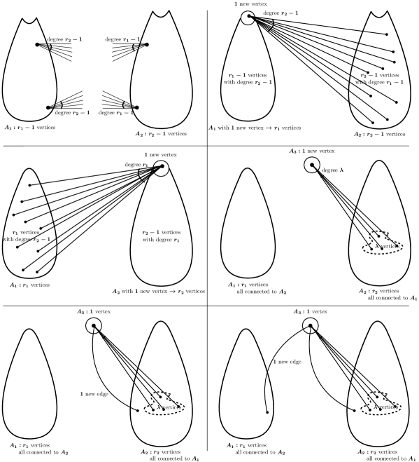
Figure 1: Stages 1-6 for Triangle Algorithm

Theorem 7.

There is a bounded-error quantum query algorithm for detecting if an $n$-vertex graph contains a triangle making $O(n^{9/7})$ many queries.

Proof.

We will show the theorem by giving a learning graph of the claimed complexity, which is sufficient by Theorem 1. We will define the learning graph by stages; let $V_{t}$ denote the $L$-vertices of the learning graph present at the beginning of stage $t$. The $L$-edges between $V_{t}$ and $V_{t+1}$ are defined in the obvious way—there is an $L$-edge between $v_{t}\in V_{t}$ and $v_{t+1}\in V_{t+1}$ if the graph labeling $v_{t}$ is a subgraph of the graph labeling $v_{t+1}$, and all such $L$-edges have weight one. The root of the learning graph is labeled by the empty graph.

For a positive input graph $G$, let $a_{1},a_{2},a_{3}$ be the vertices of a triangle of $G$. The algorithm (see Figure 1) depends on set size parameters $r_{1},r_{2}\in[n],r_{1},r_{2}=o(n)$ and a vertex degree parameter $\lambda\in[n]$ that will be optimized later. We will choose $r_{1}<r_{2}$ such that $r_{2}/r_{1}$ is an integer. The cost of each stage will be upper bounded using Lemma 3.

Stage 1 (Setup):

The initial level $V_{1}$ consists of the root of the learning graph labeled by the empty graph. The level $V_{2}$ consists of all $L$-vertices labeled by a complete unbalanced bipartite graph with disjoint color classes $A_{1},A_{2}\subseteq[n]$ where $|A_{1}|=r_{1}-1$ and $|A_{2}|=r_{2}-1$ and $r_{1}\leq r_{2}$. Flow is uniform from the root to all $L$-vertices such that $a_{i}\not\in A_{1},a_{i}\not\in A_{2}$ for $i=1,2,3$.
Cost: The hypotheses of Lemma 3 hold trivially at this stage. The length of this stage is $O(r_{1}r_{2})$. The vertex ratio is $1$, and the degree ratio is

$$\frac{{n\choose r_{1}}{n-r_{1}\choose r_{2}}}{{n-3\choose r_{1}}{n-r_{1}-3\choose r_{2}}}=O(1),$$

as $r_{1},r_{2}=o(n)$. Thus the overall cost is $O(r_{1}r_{2})$.

Stage 2 (Load $a_{1}$):

During this stage we add a vertex to the set $A_{1}$ and connect it to all vertices in $A_{2}$. Formally, $V_{3}$ consists of all vertices labeled by a complete bipartite graph between color classes $A_{1},A_{2}$ of sizes $r_{1},r_{2}-1$, respectively. The flow goes uniformly to those $L$-vertices where $a_{1}$ is the vertex added to $A_{1}$.
Cost: By the definition of stage 1, the flow is uniform over $L$-vertices at the beginning of stage 2. The out-degree of every $L$-vertex in $V_{1}$ is $n-r_{1}-r_{2}+2$. Of these, in $L$-vertices with flow, exactly one edge is taken by the flow. Thus we can apply Lemma 3. Since the degree ratio was $O(1)$ for the first stage, the vertex ratio is also $O(1)$ for this stage. The length is $r_{2}-1$. The degree ratio is $O(n)$. Thus the cost of this stage is $O(\sqrt{n}r_{2})$.

Stage 3 (Load $a_{2}$):

We add a vertex to $A_{2}$ and connect it to all of the $r_{1}$ many vertices in $A_{1}$. Thus the $L$-vertices at the end of stage $3$ consist of all complete bipartite graphs between sets $A_{1},A_{2}$ of sizes $r_{1},r_{2}$, respectively. The flow goes uniformly to those $L$-vertices where $a_{2}$ is added at this stage to $A_{2}$. Note that since we work with a complete bipartite graph, if $a_{1}\in A_{1}$ and $a_{2}\in A_{2}$ then the edge $\{a_{1},a_{2}\}$ is automatically present.
Cost: The amount of flow in a vertex with flow at the beginning of stage 3 is the same as at the beginning of stage 2, as the flow out-degree in stage 2 was one and there was no merging of flow. Thus flow is still uniform at the beginning of stage 3. The out-degree of each $L$-vertex is $n-r_{1}-r_{2}+1$ and again for $L$-vertices with flow, the flow out-degree is exactly one. Thus we can again apply Lemma 3.

The length of this stage is $r_{1}$. The vertex ratio is $O(n/r_{1})$ as flow is present in $L$-vertices where $a_{1}$ is in the set $A_{1}$ of size $r_{1}$ (and such that $a_{2},a_{3}$ are not loaded which only affects things by a $O(1)$ factor). The degree ratio is again $O(n)$ as the flow only uses $L$-edges where $a_{2}$ is added out of $n-r_{1}-r_{2}+1$ possible choices. Thus the cost of this stage is $O(\sqrt{n/r_{1}}\sqrt{n}r_{1})=O(n\sqrt{r_{1}})$.

Stage 4 (Load $a_{3}$):

We pick a vertex $v$ and $\lambda$ many edges connecting $v$ to $A_{2}$. Thus the $L$-vertices at the end of stage 4 are labeled by edges that are the union of two bipartite graphs: a complete bipartite graph between $A_{1},A_{2}$ of sizes $r_{1},r_{2}$, and a bipartite graph between $v$ and $A_{2}$ of type $\{(1,\lambda)\},\{(\lambda,1),(r_{2}-\lambda,0)\}$. Flow goes uniformly to those $L$-vertices where $v=a_{3}$ and the edge $\{a_{2},a_{3}\}$ is not loaded.
Cost: Again the amount of flow in a vertex with flow at the beginning of stage 4 is the same as at the beginning of stage 3, as the flow out-degree in stage 3 was one and there was no merging of flow. Thus the flow is still uniform. The out-degree of $L$-vertices is $(n-r_{1}-r_{2}){r_{2}\choose\lambda}$, and the flow out-degree is ${r_{2}-1\choose\lambda}$. Thus we can again apply Lemma 3.

The length of this stage is $\lambda$. At the beginning of stage 4 flow is present in those $L$-vertices where $a_{1}\in A_{1},a_{2}\in A_{2}$ and $a_{3}$ is not loaded. Thus the vertex ratio is $O((n/r_{1})(n/r_{2}))$. Finally, the degree ratio is $O(n)$. Thus the overall cost of this stage is

$$O\left(\sqrt{\frac{n}{r_{1}}}\sqrt{\frac{n}{r_{2}}}\sqrt{n}\lambda\right)=O\left(\frac{n^{3/2}\lambda}{\sqrt{r_{1}r_{2}}}\right).$$

Stage 5 (Load $\{a_{2},a_{3}\}$):

We add one new edge between $v$ and $A_{2}$. Thus the $L$-vertices at the end of this stage will be labeled by the union of edges in two bipartite graphs: a complete bipartite graph between $A_{1},A_{2}$ of sizes $r_{1},r_{2}$, and the second between $v$ and $A_{2}$ of type $\{(1,\lambda+1)\},\{(\lambda+1,1),(r_{2}-\lambda-1,0)\}$. Flow goes uniformly along those $L$-edges where the edge added is $\{a_{2},a_{3}\}$.
Cost: The flow is uniform at the beginning of this stage, as it was uniform at the beginning of stage 4, the flow out-degree was constant in stage 4, and there was no merging of flow. Each $L$-vertex has out-degree $r_{2}-\lambda$ and the flow-outdegree is one. Thus we can again apply Lemma 3.

The length of this stage is one. The vertex ratio is $O((n/r_{1})(n/r_{2})n)$ as flow is present in a constant fraction of those $L$-vertices where $a_{1}\in A_{1},a_{2}\in A_{2}$ and $v=a_{3}$. The degree ratio is $r_{2}-\lambda$, as there are this many possible edges to add and the flow uses one. Thus the overall cost of this stage is

$$O\left(\sqrt{\frac{n}{r_{1}}}\sqrt{\frac{n}{r_{2}}}\sqrt{n}\sqrt{r_{2}}\right)=O\left(\frac{n^{3/2}}{\sqrt{r_{1}}}\right).$$

Stage 6 (Load $\{a_{1},a_{3}\}$):

We add one new edge between $v$ and $A_{1}$. Thus the $L$-vertices at the end of this stage will be labeled by the union of three bipartite graphs between $A_{1},A_{2}$ and $v,A_{2}$ as before, and additionally between $v,A_{1}$ of type $\{(1,1)\},\{(1,1),(r_{1}-1,0)\}$. Flow goes uniformly on those $L$-edges where $\{a_{1},a_{3}\}$ is added.
Cost: Again flow is uniform as it was at the beginning of stage 5, the flow out-degree was constant and there was no merging. Each $L$-vertex has out degree $r_{1}$ and the flow out-degree is one. Thus we can again apply Lemma 3.

The length of this stage is one. The vertex ratio is $O((n/r_{1})(n/r_{2})n(r_{2}/\lambda))$ as flow is present in a constant fraction of those $L$-vertices where $a_{1}\in A_{1},a_{2}\in A_{2},v=a_{3}$ and $\{a_{2},a_{3}\}$ is present. The degree ratio is $r_{1}$. Thus the overall cost of this stage is

$$O\left(\sqrt{\frac{n}{r_{1}}}\sqrt{\frac{n}{r_{2}}}\sqrt{n}\sqrt{\frac{r_{2}}{\lambda}}\sqrt{r_{1}}\right)=O\left(\frac{n^{3/2}}{\sqrt{\lambda}}\right).$$

By choosing $r_{1}=n^{4/7},r_{2}=n^{5/7},\lambda=n^{3/7}$ we can make all costs, and thus their sum, $O(n^{9/7})$. ∎

To quickly compute the stage costs, it is useful to associate to each stage a local cost and global cost. The local cost is the product of the square root of the degree ratio and the length of a stage. The global cost is the square root of the factor by which the stage increases the vertex ratio—we call this a global cost as it is propagated from one stage to the next. Thus the square root of the vertex ratio at stage $t$ will be given by the product of the global costs of stages $1,\ldots,t-1$. As the cost of each stage is the product of the square root of the vertex ratio, square root of the degree ratio, and length, it can be computed by multiplying the local cost of the stage with the product of the global costs of all previous stages.

Stage	1	2	3	4	5	6
Global cost	$1$	$\sqrt{{n}/{r_{1}}}$	$\sqrt{{n}/{r_{2}}}$	$\sqrt{n}$	$\sqrt{{r_{2}}/{\lambda}}$
Local cost	$r_{1}r_{2}$	$\sqrt{n}r_{2}$	$\sqrt{n}r_{1}$	$\sqrt{n}\lambda$	$\sqrt{r_{2}}$	$\sqrt{r_{1}}$
Cost	$r_{1}r_{2}$	$\sqrt{n}r_{2}$	$n\sqrt{r_{1}}$	$n^{3/2}\lambda/\sqrt{r_{1}r_{2}}$	$n^{3/2}/\sqrt{r_{1}}$	$n^{3/2}/\sqrt{\lambda}$
Value	$n^{9/7}$	$n^{17/14}$	$n^{9/7}$	$n^{9/7}$	$n^{17/14}$	$n^{9/7}$

4 An abstract language for learning graphs

In this section we develop a high-level language for designing algorithms to detect constant-sized subgraphs, and more generally to compute functions $f:[q]^{n\times n}\rightarrow\{0,1\}$ with constant-sized $1$-certificate complexity. This high-level language consists of commands like “load a vertex” or “load an edge” that makes the algorithm easy to understand. Our main theorem, Theorem 8, compiles this high-level language into a learning graph and bounds the complexity of the resulting quantum query algorithm. After the theorem is proven, we can design quantum query algorithms using only the high-level language, without reference to learning graphs. This saves the algorithm designer from having to make many repetitive arguments as in Section 3, and also allows computer search to find the best algorithm within our framework.

4.1 Special case: subgraph containment

We now give an overview of our algorithmic framework and its implementation in learning graphs. We first use the framework for computing the function $f_{H}:[2]^{n\choose 2}\rightarrow\{0,1\}$, which is by definition $1$ if the undirected $n$-vertex input graph contains a copy of some fixed $k$-vertex graph $H=([k],E(H))$ as a subgraph. This case contains all the essential ideas; after showing this, it will be easy to generalize the theorem in few more steps to any function $f:[q]^{n\choose 2}\rightarrow\{0,1\}$ or $f:[q]^{n\times n}\rightarrow\{0,1\}$ with constant-sized $1$-certificate complexity.

Fix a positive instance $x$, and vertices $a_{1},\ldots,a_{k}\in[n]$ constituting a copy of $H$ in $x$, that is, such that $x_{\{a_{i},a_{j}\}}=1$ for all $\{i,j\}\in E(H)$. Vertices of the learning graph will be labeled by $k$-partite graphs with color classes $A_{1},\ldots,A_{k}$. The sets $A_{1},\ldots,A_{k}$ are allowed to overlap. Each $L$-vertex label will contain an undirected bipartite graph $G_{\{i,j\}}=(A_{\min\{i,j\}},A_{\max\{i,j\}},E_{\{i,j\}})$ for every edge $\{i,j\}\in E(H)$, where $E_{\{i,j\}}\subseteq A_{\min\{i,j\}}\times A_{\max\{i,j\}}$. For $\{i,j\}\in E(H)$, by $\{a_{i},a_{j}\}$ we mean $(a_{i},a_{j})$ if $i<j$, and $(a_{j},a_{i})$ if $j<i$. For an edge $\{i,j\}\in E(H)$, and $u\in[n]$, the degree of $u$ in $G_{ij}$ towards $A_{j}$ is the number of vertices in $A_{j}$ connected to $u$ if $u\in A_{i}$, and is 0 otherwise. The edges of these bipartite graphs define naturally the input edges formally required in the definition of the learning graph: for $u\neq v$, both $(u,v)$ and $(v,u)$ define the input edge $\{u,v\}$. We will disregard multiple input edges as well as self loops corresponding to edges $(u,u)$. Observe that various $L$-vertex labels may correspond to the same set of input edges. For the ease of notation we will denote $G_{\{i,j\}}$ by both $G_{ij}$ and $G_{ji}$. We will use similar convention for $E_{\{i,j\}}$ which will be denoted by both $E_{ij}$ and $E_{ji}$.

Our high-level language consists of three types of commands. The first is a setup command. This is implemented by choosing sets $A_{1},\ldots,A_{k}\subseteq[n]$ of sizes $r_{1},\ldots,r_{k}$ and bipartite graphs $G_{ij}$ between $A_{i}$ and $A_{j}$ for all $\{i,j\}\in E(H)$. Both the set sizes $r_{1},\ldots,r_{k}$ and the average degree of vertices in the bipartite graph between $A_{i}$ and $A_{j}$ are parameters of the algorithm. The degree parameter $d_{ij}=d_{ji}$ represents the average degree of vertices in the smaller of $A_{i},A_{j}$ towards the bigger one in $G_{ij}$. It is defined in this fashion so that it is always an integer and at least one—the average degree of the larger of $A_{i},A_{j}$ can be less than one. Without loss of generality there is only one setup step and it happens at the beginning of the algorithm.

The other commands allowed are to load a vertex $a_{i}$ and to load an edge $\{a_{i},a_{j}\}$ corresponding to $\{i,j\}\in E(H)$ (this terminology was introduced by Belovs). There are two regimes for loading an edge. One is the dense case, where all vertices in the graph $G_{ij}$ have a neighbor; the other is the sparse case, where some vertices in the larger of $A_{i},A_{j}$ have no neighbors in the smaller. We need to separate these two cases as they apparently have different costs (and cost analyses). The algorithm is defined by a choice of set sizes and degree parameters, and a loading schedule giving the order in which the vertices and edges are loaded and which loads all edges of $H$.

We now define the parameters specifying an algorithm more formally.

Definition 7 (Admissible parameters).

Let $H=([k],E(H))$ be a $k$-vertex graph, $r_{1},\ldots,r_{k}\in[n]$ be set size parameters, and $d_{ij}\in[n]$ for $\{i,j\}\in E(H)$ be degree parameters. Then $\{r_{i}\},\{d_{ij}\}$ are admissible for $H$ if

• $1\leq r_{i}\leq n/4$ for all $i\in[k]$,

• $\ 1\leq d_{ij}\leq\max\{r_{i},r_{j}\}$ for all $\{i,j\}\in E(H)$,

• for all $i$ there exists $j$ such that $\{i,j\}\in E(H)$ and $d_{ij}(2r_{j}+1)/(2r_{i}+1)\geq 1$.

We give a brief explanation of the purpose of each of these conditions. We will encounter terms of the form ${n\choose r_{i}}/{n-k\choose r_{i}}$ that we wish to be $O(1)$; this is ensured by the first condition. As $d_{ij}$ represents the average degree of the vertices in the smaller of $A_{i},A_{j}$ towards the larger, the second condition states that this degree cannot be larger than the number of distinct possible neighbors. The third item ensures that the average degree of vertices in $A_{i}$ is at least one in the bipartite graph with some $A_{j}$.

Definition 8 (Loading schedule).

Let $H=([k],E(H))$ be a $k$-vertex graph with $m$ edges. A loading schedule for $H$ is a sequence $S=s_{1}s_{2}\ldots s_{k+m}$ whose elements $s_{i}\in[k]$ or $s_{i}\in E(H)$ are vertex labels or edge labels of $H$ such that an edge $\{i,j\}$ only appears in $S$ after $i$ and $j$, and $S$ contains all edges of $H$. Let $\mathrm{VS}_{t}$ be the set of vertices in $S$ before position $t$ and similarly $\mathrm{ES}_{t}$ the set of edges in $S$ before position $t$.

We can now state the main theorem of this section.

Theorem 8.

Let $H=([k],E(H))$ be a $k$-vertex graph. Let $r_{1},\ldots,r_{k},d_{ij}$ be admissible parameters for $H$, and $S$ be a loading schedule for $H$. Then the quantum query complexity of determining if an $n$-vertex graph contains $H$ as a subgraph is at most a constant times the maximum of the following quantities:

• Setup cost:

  $$\sum_{\{u,v\}\in E(H)}\min\{r_{u},r_{v}\}d_{uv},$$

• Cost of loading $s_{t}=i$:

  $$\left(\prod_{u\in\mathrm{VS}_{t}}\sqrt{\frac{n}{r_{u}}}\prod_{\{u,v\}\in\mathrm{ES}_{t}}\sqrt{\frac{\max\{r_{u},r_{v}\}}{d_{uv}}}\right)\times\sqrt{n}\left(\sum_{\begin{subarray}{c}j:\{i,j\}\in E(H)\\ r_{i}\leq r_{j}\end{subarray}}d_{ij}+\sum_{\begin{subarray}{c}j:\{i,j\}\in E(H)\\ r_{i}>r_{j}\end{subarray}}\frac{r_{j}d_{ij}}{r_{i}}\right),$$

• Cost of loading $s_{t}=\{i,j\}$ in the dense case where $(2\min\{r_{i},r_{j}\}+1)d_{ij}\geq(2\max\{r_{i},r_{j}\}+1)$:

  $$\left(\prod_{u\in\mathrm{VS}_{t}}\sqrt{\frac{n}{r_{u}}}\prod_{\{u,v\}\in\mathrm{ES}_{t}}\sqrt{\frac{\max\{r_{u},r_{v}\}}{d_{uv}}}\right)\max\{r_{i},r_{j}\},$$

• Cost of loading $s_{t}=\{i,j\}$ in the sparse case where $(2\min\{r_{i},r_{j}\}+1)d_{ij}<(2\max\{r_{i},r_{j}\}+1)$:

  $$\left(\prod_{u\in\mathrm{VS}_{t}}\sqrt{\frac{n}{r_{u}}}\prod_{\{u,v\}\in\mathrm{ES}_{t}}\sqrt{\frac{\max\{r_{u},r_{v}\}}{d_{uv}}}\right)\sqrt{r_{i}r_{j}}.$$

If $\{i,j\}$ is loaded in the dense case we call it a type 1 edge, and if it loaded in the sparse case we call it a type 2 edge. The costs of a stage given by Theorem 8 can again be understood more simply in terms of local costs and global costs. We give the local and global cost for each stage in the table below.

Stage	Global Cost	Local Cost
Setup	1	$\sum_{\{u,v\}\in H}\min\{r_{u},r_{v}\}d_{uv}$
Load vertex $i$	$\sqrt{n/r_{i}}$	$\sqrt{n}\times\text{total degree of }i$
Load a type 1 edge $\{i,j\}$	$\sqrt{\max\{r_{i},r_{j}\}/d_{ij}}$	$\max\{r_{i},r_{j}\}$
Load a type 2 edge $\{i,j\}$	$\sqrt{\max\{r_{i},r_{j}\}/d_{ij}}$	$\sqrt{r_{i}r_{j}}$

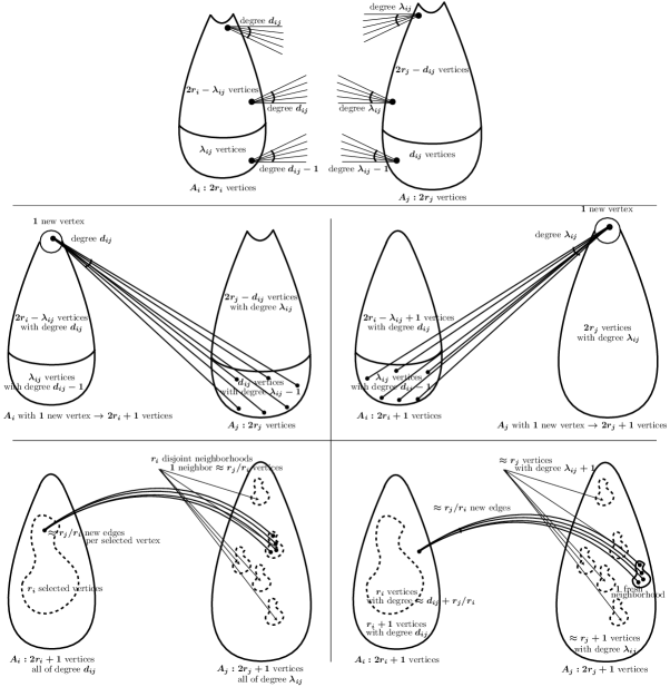
Figure 2: Example of a part of learning graph corresponding to Case 1 and restricted to the bipartite graph between $A_{i}$ and $A_{j}$, where $r_{i}<r_{j}$. Observe that $\lambda_{ij}\approx\frac{r_{i}}{r_{j}}d_{ij}$. The loading schedule is ’setup’, ’load $i$’, ’load $j$’ and ’load $\{i,j\}$’.

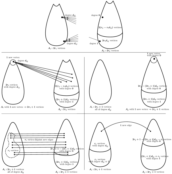
Figure 3: Similar to Figure 2, but for Case 2.

Proof.

We show the theorem by giving a learning graph of the stated complexity. Vertices of the learning graph will be labeled by $k$-partite graphs with color classes $A_{1},\ldots,A_{k}$ of cardinality (of order) $r_{1},\ldots,r_{k}\in[n]$. The parameter $d_{ij}\geq 1$ is the average degree of vertices in the smaller of $A_{i},A_{j}$ towards the bigger in the bipartite graph $G_{ij}$.

The bipartite graph $G_{ij}$, for each edge $\{i,j\}\in E(H)$, will be specified by its type, that is by its degree sequences as given in Definition 2.

We first need to modify the set size parameters $\{r_{i}\}$ to satisfy a technical condition. Let $r_{i_{1}}\leq\cdots\leq r_{i_{k}}$ be a listing in increasing order. We set $r_{i_{1}}^{\prime}=r_{i_{1}}$ and $r_{i_{t}}^{\prime}=\Theta(r_{i_{t}})$ such that $(2r_{i_{t}}^{\prime}+1)/(2r_{i_{t-1}}^{\prime}+1)$ is an odd integer. As a consequence, $(2\max\{r_{i}^{\prime},r_{j}^{\prime}\}+1)/(2\min\{r_{i}^{\prime},r_{j}^{\prime}\}+1)$ is an odd integer, for every $i\neq j$. We now suppose this is done and drop the primes.

Throughout the construction of the learning graph we will deal with two cases for the bipartite graph between $A_{i}$ and $A_{j}$, depending on the size and degree parameters.

• Case 1 is where $(2\min\{r_{i},r_{j}\}+1)d_{ij}\geq 2\max\{r_{i},r_{j}\}+1$, which means that there are enough edges from the smaller of $A_{i},A_{j}$ to cover the larger. We will say that the parameters for $\{i,j\}$ are of type 1. In this case, we take $d_{ij}^{\prime}=\Theta(d_{ij})$ to be such that

  $$2d_{ij}^{\prime}+1=(2\lambda_{ij}+1)\frac{2\max\{r_{i},r_{j}\}+1}{2\min\{r_{i},r_{j}\}+1}$$ (2)

  for some integer $\lambda_{ij}$. This can be done as $(2\max\{r_{i},r_{j}\}+1)/(2\min\{r_{i},r_{j}\}+1)$ is an odd integer. In our construction, $\lambda_{ij}$ will be the average degree of the vertices in the larger of $A_{i},A_{j}$ towards the smaller, which we want to be integer. We now consider this done and drop the primes.

• Case 2 is where $(2\min\{r_{i},r_{j}\}+1)d_{ij}<2\max\{r_{i},r_{j}\}+1$. We will say that the parameters for $\{i,j\}$ are of type 2. In this case, all degrees of vertices in the larger of $A_{i},A_{j}$ towards the smaller will be either zero or one.

Now we are ready to describe the learning graph. Figures 2 and 3 illustrate the evolution of a learning graph for a subsequence $(i,j,\{i,j\})$ of some loading schedule, that is the sequence of instructions ‘setup’, ‘load $i$’, ‘load $j$’ and ‘load $\{i,j\}$’. The figures only represent the added edges between $A_{i}$ and $A_{j}$, where $r_{i}<r_{j}$. Figure 2 corresponds to Case 1, and Figure 3 to Case 2.

Recall that for every positive instance $x$, we fixed $a_{1},\ldots,a_{k}\in[n]$ be such that $x_{\{a_{u},a_{v}\}}=1$ for all $\{u,v\}\in E(H)$. During the construction we will specify for every edge $\{u,v\}\in E(H)$, and for every stage number $t$, the correct degree $\mathrm{cd}(u,v,t)$ which is the degree of $a_{u}$ in $G_{ij}$ towards $a_{v}$ in each $L$-vertex of $V_{t+1}$ with positive flow.

Stage 0 (Setup):

For each edge $\{i,j\}\in E(H)$ we setup a bipartite graph between $A_{i}$ and $A_{j}$. The type of the bipartite graph depends on the type of the parameters for $\{i,j\}$. Let $\ell=\min\{r_{i},r_{j}\}$ and $g=\max\{r_{i},r_{j}\}$.

• Case 1: Solving for $\lambda_{ij}$ in Equation (2) we get $\lambda_{ij}=((2\ell+1)d_{ij}+\ell-g)/(2g+1)$. Intuitively, $d_{ij}$ represents the average degree of vertices in the smaller of $A_{i},A_{j}$ and $\lambda_{ij}$ the average degree in the larger. Formally, the type of bipartite graph between $A_{i},A_{j}$, with the listing of degrees for the smaller set given first, is $(\{(2\ell-\lambda_{ij},d_{ij}),(\lambda_{ij},d_{ij}-1)\},\{(2g-d_{ij},\lambda_{ij}),(d_{ij},\lambda_{ij}-1)\})$.

• Case 2: In this case the type of bipartite graph between $A_{i}$ and $A_{j}$, with the listing of degrees for the smaller set given first, is $(\{(2\ell,d_{ij})\},\{(2\ell d_{ij},1),(2g-2\ell d_{ij},0)\})$.

The $L$-vertices at the end of stage $0$ will be labeled by (possibly overlapping) sets $A_{1},\ldots,A_{k}$ of sizes $r_{1},\ldots,r_{k}$ and edges corresponding to a graph of the appropriate type between $A_{i}$ and $A_{j}$ for all $\{i,j\}\in E(H)$. Flow goes uniformly to those $L$-vertices where none of $a_{1},\ldots,a_{k}$ are in any of the sets $A_{1},\ldots,A_{k}$. For all $\{u,v\}\in E(H)$, we set $\mathrm{cd}(u,v,0)=0$.

Stage $t$ when $s_{t}=i$:

In this stage we load $a_{i}$. The $L$-edges in this stage select a vertex $v$ and add it to $A_{i}$. For all $j$ such that $\{i,j\}\in E(H)$ we add the following edges:

• Case 1: Say the parameters for $\{i,j\}$ are of type 1. If $r_{i}\leq r_{j}$, then $v$ is connected to those vertices of degree $\lambda_{ij}-1$ in $A_{j}$, and we set $\mathrm{cd}(i,j,t)=d_{ij}$. Otherwise $v$ is connected to those vertices of degree $d_{ij}-1$ in $A_{j}$, and we set $\mathrm{cd}(i,j,t)=\lambda_{ij}$.

• Case 2: Say the parameters for $\{i,j\}$ are of type 2. If $r_{i}\leq r_{j}$ then $v$ is connected to $d_{ij}$ vertices of degree 0 in $A_{j}$, and we set $\mathrm{cd}(i,j,t)=d_{ij}$. Else no edges are added between $v$ and $A_{j}$, and we set $\mathrm{cd}(i,j,t)=0$.

For all other $(u,v)$, we set $\mathrm{cd}(u,v,t)=\mathrm{cd}(u,v,t-1)$. Flow goes uniformly on those $L$-edges where $v=a_{i}$.

Stage $t$ when $s_{t}=\{i,j\}$:

In this stage we load $\{a_{i},a_{j}\}$. Again we break down according to the type of the parameters for $\{i,j\}$. Let $\ell=\min\{r_{i},r_{j}\}$ and $g=\max\{r_{i},r_{j}\}$.

• Case 1: As both $a_{i}$ and $a_{j}$ have been loaded, between $A_{i}$ and $A_{j}$ there is a bipartite graph of type $(\{(2\ell+1,d_{ij})\},\{(2g+1,\lambda_{ij})\})$, with the degree listing of the smaller set coming first. If we simply added $\{a_{i},a_{j}\}$ at this step, $a_{i}$ and $a_{j}$ would be uniquely identifiable by their degree and blow up the complexity of later stages.

  To combat this, loading $\{a_{i},a_{j}\}$ will consist of two substages $t.I$ and $t.II$. The first substage is a hiding step, done to reduce the complexity of having $\{a_{i},a_{j}\}$ loaded. Then we actually load $\{a_{i},a_{j}\}$.

  Substage $t.I$: Let $h=(2g+1)/(2\ell+1)$. We select $\ell$ vertices in the smaller of $A_{i},A_{j}$, and to each of these add $h$ many neighbors. All neighbors chosen in this stage are distinct. Thus at the end of this stage the type of bipartite graph between $A_{i}$ and $A_{j}$ is $(\{(\ell,d_{ij}+h),(\ell+1,d_{ij})\},\{(\ell(2g+1)/(2\ell+1),\lambda_{ij}+1),((2g+1)(1-\ell/(2\ell+1)),\lambda_{ij})\})$. Flow goes uniformly along those $L$-edges where neither $a_{i}$ nor $a_{j}$ receive any new edges. For all $\{u,v\}\in E(H)$, we set $\mathrm{cd}(u,v,t+1)=\mathrm{cd}(u,v,t)$.

  Substage $t.II$: The $L$-edges in this substage select a vertex $u$ in the smaller of $A_{i},A_{j}$ of degree $d_{ij}$ and add $h$ many neighbors of degree $\lambda_{ij}$. Flow goes uniformly along those $L$-edges where $u\in\{a_{i},a_{j}\}$ and $\{a_{i},a_{j}\}$ is one of the edges added. Let $s$ be the index of the smaller of the sets $A_{i},A_{j}$, and let $b$ the other index. We set $\mathrm{cd}(s,b,t+1)=d_{ij}+h,\mathrm{cd}(b,s,t+1)=\lambda_{ij}+1$ and $\mathrm{cd}(u,v,t+1)=\mathrm{cd}(u,v,t)$ for $\{u,v\}\neq\{i,j\}$.

• Case 2: As both $a_{i}$ and $a_{j}$ have been loaded, there is a bipartite graph of type $(\{(2\ell+1,d_{ij})\},\{((2\ell+1)d_{ij},1),(2g+1-(2\ell+1)d_{ij},0)\})$. We again first do a hiding step, and then add the edge $\{a_{i},a_{j}\}$.

  Substage $t.I$: We select $\ell$ vertices in the smaller of $A_{i},A_{j}$ and to each add a single edge to a vertex of degree zero in the larger of $A_{i},A_{j}$. Flow goes uniformly along those $L$-edges where no edges adjacent to $a_{i},a_{j}$ are added. For all $\{u,v\}\in E(H)$, we set $\mathrm{cd}(u,v,t+1)=\mathrm{cd}(u,v,t)$.

  Substage $t.II$: A single edge is added between a vertex in the smaller of $A_{i},A_{j}$ of degree $d_{ij}$ and a vertex in the larger of $A_{i},A_{j}$ of degree zero. Flow goes along those $L$-edges where $\{a_{i},a_{j}\}$ is added. Let again $s$ be the index of the smaller of the sets $A_{i},A_{j}$, and let $b$ the other index. We set $\mathrm{cd}(s,b,t+1)=d_{ij}+1,\mathrm{cd}(b,s,t+1)=1$ and $\mathrm{cd}(u,v,t+1)=\mathrm{cd}(u,v,t)$ for $\{u,v\}\neq\{i,j\}$.

This completes the description of the learning graph.

Complexity analysis

We will use Lemma 4 to evaluate the complexity of each stage. First we need to establish the hypothesis of this lemma, which we will do using Lemma 5 and Lemma 6. Remember that given $\sigma\in S_{n}$, we defined and denoted by $\sigma$ the permutation over $[n]\times[n]$ such that $\sigma(i,j)=(\sigma(i),\sigma(j))$. First of all let us observe that every $\sigma\in S_{n}$ is in the automorphism group of the function we are computing, since it maps a 1-certificate into a 1-certificate. As the flow only depends on the 1-certificate graph, this implies that $S_{n}$ acts transitively on the flows and therefore we obtain the conclusion of Lemma 5.

Let $V_{t}$ stand for the $L$-vertices at the beginning of stage $t$. For a positive input $x$, and for an $L$-vertex $P\in V_{t}$, we will denote the incoming flow to $P$ on $x$ by $p_{x}(P)$ and the number of outgoing edges from $P$ with positive flow on $x$ by $g_{x}^{+}(P)$. For an $L$-vertex $R\in V_{t-1}$ we will denote by $g_{x,R}^{-}(P)$ number of incoming edges to $P$ from $L$-vertices of the isomorphism type of $R$ with positive flow on $x$, that is $g_{x,R}^{-}(P)=|\{\tau\in S_{n}:p_{x}(\tau(R),P)\neq 0\}|$. The crucial features of our learning graph construction are the following: at every stage, for every $L$-vertex $P$ and every $\sigma\in S_{n}$, the $L$-vertex $\sigma(P)$ is also present. The outgoing flow from an $L$-vertex is always uniformly distributed among the edges getting flow. The flow depends only on the vertices in the input containing a copy of the graph $H$, and therefore the values $g_{x}^{+}(P)$ and $g_{x,R}^{-}(P)$, for $p_{x}(P)$ non-zero, depend only on the isomorphism types of $P$ and $R$. Mathematically, this last property translates to: for all $t$, for all $P\in V_{t}$, for all $R\in V_{t-1}$, for all positive inputs $x$ and $y$, for all $\sigma\in S_{n}$, we have

$$[p_{x}(P)\neq 0\mbox{{\rm~{}and~{}}}p_{y}(\sigma(P))\neq 0]\ \ \ \Longrightarrow\ \ \ [g_{x}^{+}(P)=g_{y}^{+}(\sigma(P))\mbox{{\rm~{}and~{}}}g_{x,R}^{-}(P)=g_{y,R}^{-}(\sigma(P))].$$ (3)

which is exactly the hypothesis of Lemma 6.

Now we have established the hypotheses of Lemma 4 and turn to evaluating the bound given there. The main task is evaluating the maximum vertex ratio of each stage. The general way we will do this is to consider an arbitrary vertex $P$ of a stage. We then lower bound the probability that $\sigma(P)$ is in the flow for a positive input $x$ and a random permutation $\sigma\in S_{n}$, without using any particulars of $P$. This will then upper bound the maximum vertex ratio. We use the notation $P\in F_{x}$ to denote that $L$-vertex $P$ has at least one incoming edge with flow on input $x$.

Lemma 9 (Maximum vertex ratio).

For any $L$-vertex $P\in V_{t+1}$ and any positive input $x$

$$\Pr_{\sigma}[\sigma(P)\in F_{x}]=\Omega\left(\prod_{j\in\mathrm{VS}_{t}}\frac{r_{j}}{n}\prod_{(u,v)\in\mathrm{ES}_{t}}\frac{d_{uv}}{\max\{r_{u},r_{v}\}}\right).$$

Proof.

We claim that an $L$-vertex $P$ in $V_{t+1}$, that is at the end of stage $t$, has flow if and only if

$$\forall i\in\mathrm{VS}_{t},~{}\forall\{i,j\}\in\mathrm{ES}_{t},\text{~{}we~{}have~{}}a_{i}\in A_{i}\mbox{{\rm~{}and~{}}}\{a_{i},a_{j}\}\in E_{ij},$$ (4)

$$\forall i\in[k]\setminus\mathrm{VS}_{t},~{}\forall\{i,j\}\in H(E)\setminus\mathrm{ES}_{t},\text{~{}we~{}have~{}}a_{i}\not\in A_{i}\text{~{}and~{}}\{a_{i},a_{j}\}\not\in E_{ij},$$ (5)

$$\forall\{i,j\}\in\mathrm{ES}_{t},\text{~{}the~{}degree~{}of~{}}a_{i}\mbox{{\rm~{}in ~{}}}G_{ij}\text{~{}towards ~{}}A_{j}\text{~{}is ~{}}\mathrm{cd}(i,j,t).$$ (6)

The only if part of the claim is obvious by the construction of the learning graph. The if part can be proven by induction on $t$. For $t=0,$ the first half (5) is exactly the one which defines the flow for $L$-vertices in $V_{1}$.

For the inductive step let us suppose first that $s_{t}=i$. Consider the label $P^{\prime}$ by dropping the vertex $a_{i}$ from $A_{i}$. Then in $P^{\prime}$ every bipartite graph is of appropriate type for level $t$ because of (6), and therefore $P^{\prime}\in V_{t}$. It is easy to check that $P^{\prime}$ also satisfies all three conditions, (for (6) we also have to use the second half of (5): $\{a_{i},a_{j}\}\not\in E_{ij}$), and therefore has positive flow. Since $P^{\prime}$ is a predecessor of $P$ is the learning graph, $P$ has also positive flow.

Now let us suppose that $s_{t}=\{i,j\}$. In $P$ the edge set $E_{ij}$ can be decomposed into the disjoint union of $E_{1}\cup E_{2}$, where $E_{1}$ a bipartite graph of type $(\{(2\ell+1,d_{ij})\},\{(2g+1,\lambda_{ij})\})$ and $E_{2}$ is of type $(\{(\ell+1,h),(\ell,0\},\{((\ell+1)h,1),(2g+1-(\ell+1)h,0)\})$, and (6) implies that $\{a_{i},a_{j}\}\in E_{2}$. Consider the label $P^{\prime}$ by dropping the edges of $E_{2}$ from $E_{ij}$. Again, $P^{\prime}$ satisfies the inductive hypotheses, and therefore gets positive flow, which implies the same for $P$.

Suppose now that the $L$-vertex $P$ is labeled by sets $A_{1},\ldots,A_{k}$ (some may be empty) and let the set of edges between $A_{i}$ and $A_{j}$ be $E_{ij}$. We want to lower bound the probability that $\sigma(P)\in F_{x}$, meaning that $\sigma(P)$ satisfies the above three conditions. Item (5) is always satisfied with constant probability; moreover, conditioned on item (5) the probability of the other events does not decrease. Thus we take this constant factor loss and focus on the items (4), (6).

We also claim that, conditioned on item (4) holding, item (6) holds with constant probability. This can be seen as in the hiding step, in both case 1 and case 2, the probability that $a_{i},a_{j}$ have the correct degree given that they are loaded is at least $1/4$. In the step of loading an edge, again in case 1 half the vertices on the left and right hand sides have the correct degree and so this probability is again $1/4$; in case 2, given that the edge is loaded, whichever of $a_{i},a_{j}$ is in the larger set will automatically have the correct degree, and the other one will have correct degree with probability $1/2$. Now we take this constant factor loss to obtain that $\Pr_{\sigma}[\sigma(P)\in F_{x}]$ is lower bounded by a constant factor times the probability that item (4) holds.

The events in the first condition are independent, except that for the edge $\{a_{i},a_{j}\}$ to be loaded the vertices $a_{i}$ and $a_{j}$ have to be also loaded. Thus we can lower bound the probability it is satisfied by

$$\Pr_{\sigma}[\sigma(P)\in F_{x}]=\Omega\Big{(}\prod_{i\in VS_{t}}\Pr_{\sigma}[a_{i}\in\sigma(A_{i})]\times\!\!\!\prod_{(u,v)\in ES_{t}}\Pr_{\sigma}[\{a_{i},a_{j}\}\in\sigma(E_{ij})|a_{i}\in\sigma(A_{i}),a_{j}\in\sigma(A_{j})]\Big{)}$$

Now $\Pr_{\sigma}[a_{i}\in\sigma(A_{i})]=\Omega(r_{i}/n)$ as this fraction of permutations will put $a_{i}$ into a set of size $r_{i}$. For the edges we use the following lemma.

Lemma 10.

Let $Y_{1},Y_{2}\subseteq[n]$ be of size $\ell,g$ respectively, and let $(y_{1},y_{2})\in Y_{1}\times Y_{2}$. Let $K$ be a bipartite graph between $Y_{1}$ and $Y_{2}$ of type $\{(\ell,d)\},\{(g,\ell d/g)\}$. Then $\Pr_{\sigma}[\{y_{1},y_{2}\}\in\sigma(K)=d/g$.

Proof.

Because of symmetry, this probability does not depend on the choice of $\{y_{1},y_{2}\}$; denote it by $p$. Let $K_{1},\ldots,K_{c}$ be an enumeration of all bipartite graphs isomorphic to $K$. We will count in two different ways the cardinality $\chi$ of the set $\{(e,h):e\in K_{h}\}$. Every $K_{h}$ contains $\ell d$ edges, therefore $\chi=c\ell d$. On the other hand, every edge appears in $pc$ graphs, therefore $\chi=\ell gpc$, and thus $p=d/g$. ∎

In our case, the graph $G_{ij}$ as in the hypothesis of the lemma plus some additional edges. By monotonicity, it follows that

$$\Pr_{\sigma}[\{a_{i},a_{j}\}\in\sigma(E_{ij})|a_{i}\in\sigma(A_{i}),a_{j}\in\sigma(A_{j})]=\Omega(d_{ij}/\max\{r_{i},r_{j}\}).$$

∎

This analysis is common to all the stages. Now we go through each type of stage in turn to evaluate the stage specific length and degree ratio.

Setup Cost:

The length of this stage is upper bounded by

$$\sum_{(i,j)\in E(H)}\min\{r_{i},r_{j}\}d_{ij}.$$

We can upper bound the degree ratio by

$$\prod_{i\in[k]}\frac{{n\choose 2r_{i}}}{{n-k\choose 2r_{i}}}\leq 2^{k}=O(1)$$

as $r_{i}<n/4$.

Stage $t$ when $s_{t}=i$:

In a stage loading a vertex the degree ratio is $O(n)$ as there are $n-r_{i}$ possible vertices to add yet only one is used by the flow. The length of this stage is the total degree which is upper bounded by

$$\sum_{\begin{subarray}{c}j:\{i,j\}\in E(H)\\ r_{i}\leq r_{j}\end{subarray}}d_{ij}+\sum_{\begin{subarray}{c}j:\{i,j\}\in E(H)\\ r_{i}>r_{j}\end{subarray}}\frac{r_{j}d_{ij}}{r_{i}}.$$

Stage $t$ when $s_{t}=\{i,j\}$:

Technically we should analyze the complexity of the two substages as two distinct stages. However, as we will see, in both cases the degree ratio in the first substage is $O(1)$, and therefore the local cost of this stage is just the maximum of the local cost of the two substages.

Stage $t.I$:

In Case 1, the length of this stage is $O(\max\{r_{i},r_{j}\})$ and the degree ratio is constant. In Case 2, the length of this stage is $O(\min\{r_{i},r_{j}\})$ and the degree ratio is constant.

Stage $t.II$:

In Case 1, the length is $h=O(\max\{r_{i},r_{j}\}/\min\{r_{i},r_{j}\})$. The degree ratio is of order $\ell\frac{{g\choose h}}{{g-1\choose h-1}}=O(\ell^{2})$. Thus the square root of the degree ratio times the length is of order $\max\{r_{i},r_{j}\}$.

In Case 2, the length is one and the degree ratio is $O(r_{i}r_{j})$ as there are $O(r_{i}r_{j})$ many possible edges that could be added and the flow uses one.

Thus in Case 1 in both substages the product of the length and square root of degree ratio is $O(\max\{r_{i},r_{j}\})$. In Case 2, substage II dominates the complexity where the product of the length and square root of degree ratio is $O(\sqrt{r_{i}r_{j}})$. ∎

4.2 Extensions and basic properties

We now extend Theorem 8 to the general case of computing a function $f:[q]^{n\times n}\rightarrow\{0,1\}$ with constant-sized $1$-certificates. A certificate graph for such a function will be a directed graph possibly with self-loops. Between $i$ and $j$ there can be bidirectional edges, that is both $(i,j)$ and $(j,i)$ present in the certificate graph, but there will not be multiple edges between $i$ and $j$, as there are no repetitions of indices in a certificate.

We start off by modifying the algorithm of Theorem 8 to work for detecting directed graphs with possible self-loops. To do this, the following transformation will be useful.

Definition 9.

Let $H$ be a directed graph, possibly with self-loops. The undirected version $U(H)$ of $H$ is a simple undirected graph formed by eliminating any self-loops in $H$, and making all edges of $H$ undirected and single.

Lemma 11.

Let $H$ be a directed $k$-vertex graph, possibly with self loops. Then the quantum query complexity of detecting if an $n$-vertex directed graph $G$ contains $H$ as a subgraph is at most a constant times the complexity given in Theorem 8 of detecting $U(H)$ in an $n$-vertex undirected graph.

Proof.

Let $H$ be a directed $k$-vertex graph (possibly with self-loops) and $H^{\prime}=U(H)$ be its undirected version. Let $r_{1},\ldots,r_{k},d_{ij}$ be admissible parameters for $H^{\prime}$, and $S$ a loading schedule for $H^{\prime}$. Fix a directed $n$-vertex graph $G$ containing $H$ as a subgraph. Let $a_{1},\ldots,a_{k}$ be vertices of $G$ such that $(a_{i},a_{j})\in E(G)$ for $(i,j)\in E(H)$. We convert the algorithm for loading $H^{\prime}$ in Theorem 8 into one for loading $H$ of the same complexity.

The setup step for $H^{\prime}$ is modified as follows. In the bipartite graph between $A_{i}$ and $A_{j}$, if both $(i,j),(j,i)\in E(H)$ then all edges between $A_{i}$ and $A_{j}$ are directed in both directions; otherwise, if $(i,j)\in E(H)$ or $(j,i)\in E(H)$ they are directed from $A_{i}$ to $A_{j}$ or vice versa, respectively. For every self-loop in $H$, say $(i,i)\in E(H)$, we add self-loops to the vertices in $A_{i}$. Note that these modifications at most double the number of edges added, and hence the cost, of the setup step.

Loading a vertex: When loading $a_{i}$ we connect it as before, now orienting the edges according to $(i,j)$ or $(j,i)$ in $E(H)$, or both. If $(i,i)\in E(H)$, then we add a self loop to $a_{i}$. The only change in the complexity of this stage is again the length, which at most doubles. Notice that in the case of a self-loop we have also already loaded the edge $(a_{i},a_{i})$. We do not incur an extra cost for loading this edge, however, as the self loop is loaded if and only if the vertex is.

Loading an edge: Say that we are at the stage where $s_{t}=\{i,j\}\in E(H^{\prime})$. If exactly one of $(i,j),(j,i)\in E(H)$ then this step happens exactly as before, except that the bipartite graph has edges directed from $A_{i}$ to $A_{j}$ or vice versa, respectively. If both $(i,j)$ and $(j,i)\in E(H)$, then in this step all edges added are bidirectional. This again at most doubles the length, and does not affect the degree flow probability as $(a_{i},a_{j})$ is loaded if and only if $(a_{j},a_{i})$ is loaded as all edges are bidirectional. ∎

Lemma 12.

Let $f:[q]^{n\times n}\rightarrow\{0,1\}$ be a function such that all minimal $1$-certificate graphs are isomorphic to a directed $k$-vertex graph $H$. Then the quantum query complexity of computing $f$ is at most the complexity of detecting $H$ in an $n$-vertex graph, as given by Lemma 11.

Proof.

We will show the theorem by giving a learning graph algorithm. Let $\mathcal{G}=(\mathcal{V},\mathcal{E},S,w,\{p_{y}\})$ be the learning graph from Lemma 11 for $H$. All of $\mathcal{V},\mathcal{E},S,w$ will remain the same in our learning graph $\mathcal{G}^{\prime}$ for $f$. We now describe the definition of the flows in $\mathcal{G}^{\prime}$.

Consider a positive input $x$ to $f$, and let $\alpha$ be a minimal $1$-certificate for $x$ such that the certificate graph $H_{\alpha}$ is isomorphic to $H$. The flow $p_{x}$ will be defined as the flow for $H_{\alpha}$ (thought of as an $n$-vertex graph, thus with $n-k$ isolated vertices) in $\mathcal{G}$, the learning graph for detecting $H$. This latter flow has the property that the label of every terminal of flow contains $E(H_{\alpha})$ and thus will also contain the index set of a $1$-certificate for $x$.

The positive complexity of the learning graph for $f$ will be the same as that for detecting $H$ and the negative complexity will be at most that as in the learning graph for detecting $H$, thus we conclude that the complexity of computing $f$ is at most that for detecting $H$ as given in Lemma 11. ∎

Theorem 13.

Say that the $1$-certificate complexity of $f:[q]^{n\times n}\rightarrow\{0,1\}$ is at most a constant $m$, and let $H_{1},\ldots,H_{c}$ be the set of graphs (on at most $m$ edges) for which there is some positive input $x$ such that $H_{i}$ is a minimal $1$-certificate graph for $x$. Then the quantum query complexity of computing $f$ is at most a constant times the maximum of the complexities of detecting $H_{i}$ for $i=1,\ldots,c$ as given by Lemma 11.

Proof.

Consider learning graphs $\mathcal{G}_{1},\ldots,\mathcal{G}_{c}$ given by Lemma 11 for detecting $H_{1},\ldots,H_{c}$ respectively. Further suppose these learning graphs are normalized such that their negative and positive complexities are equal.

We construct a learning graph $\mathcal{G}$ for $f$ where the edges and vertices are given by connecting a new root node by an edge of weight one to the root nodes of each of $\mathcal{G}_{1},\ldots,\mathcal{G}_{c}$. Thus the negative complexity of $\mathcal{G}$ is at most $c(1+\max_{i}C_{0}(\mathcal{G}_{i})$.

Now we construct the flow for a positive input $x$. Let $\alpha$ be a minimal $1$-certificate for $x$ such that the certificate graph $H_{\alpha}$ is isomorphic to $H_{i}$, for some $i$. Then the flow on $x$ is first directed entirely to the root node of $\mathcal{G}_{i}$. It is then defined within $\mathcal{G}_{i}$ as in Lemma 12. Thus the positive complexity of $\mathcal{G}$ is at most $c(1+\max_{i}C_{1}(\mathcal{G}_{i}))$. ∎

To make Theorem 8 and Lemma 11 easier to apply, here we establish some basic intuitive properties about the complexity of the algorithm for different subgraphs. Namely, we show that if $H^{\prime}$ is a subgraph of $H$ then the complexity given by Lemma 11 for detecting $H^{\prime}$ is at most that of $H$. We show a similar statement when $H^{\prime}$ is a vertex contraction of $H$.

Lemma 14.

Let $H$ be a directed $k$-vertex graph (possibly with self-loops) and $H^{\prime}$ a subgraph of $H$. Then the quantum query complexity of determining if an $n$-vertex graph $G$ contains $H^{\prime}$ is at most that of determining if $G$ contains $H$ from Lemma 11.

Proof.

Assume that the vertices of $H$ are labeled from $[k]$ and that $H^{\prime}$ is labeled such $(i,j)\in E(H)$ for all $(i,j)\in E(H^{\prime})$.

The learning graph we use for detecting $H^{\prime}$ is the same as that for $H$. For a graph $G$ containing a $H^{\prime}$ as a subgraph, let $a_{1},\ldots,a_{k}$ be such that $(a_{i},a_{j})\in G$ for all $(i,j)\in H^{\prime}$. (If $t$ is an isolated vertex in $H^{\prime}$, then $a_{t}$ can be chosen arbitrarily). The flow for $G$ is defined in the same way as in the learning graph for $H$. Note that once $a_{1},\ldots,a_{k}$ have been identified, the definition of flow depends only edge slots—not on edges—thus this definition remains valid for $H^{\prime}$. Furthermore all terminals of flow are labeled by edge slots $(a_{i},a_{j})$ for all $(i,j)\in H$, and so also contain the edge slots for $H^{\prime}$. Thus this is a valid flow for detecting $H^{\prime}$. As the learning graph and flow are the same, the complexity will be as that given in Lemma 11. ∎

Lemma 15.

Let $H$ be a $k$-vertex graph and $H^{\prime}$ a vertex contraction of $H$. Then the quantum query complexity of detecting $H^{\prime}$ is at most that of detecting $H$ given in Lemma 11.

Proof.

Again we assume that the vertices of $H$ are labeled from $[k]$. The key point is the following: if $H^{\prime}$ is a vertex contraction of $H$, then there are $z_{1},\ldots,z_{k}\in[k]$ (not necessarily distinct) such that $(z_{i},z_{j})\in E(H^{\prime})$ if and only if $(i,j)\in E(H)$. The learning graph for $H^{\prime}$ will be the same as that for $H$ except for the flows. For a graph $G$ containing $H^{\prime}$, we choose vertices $a_{1},\ldots,a_{k}$ (not necessarily distinct) such that if $(z_{i},z_{j})\in E(H^{\prime})$ then $(a_{i},a_{j})\in E(G)$. As $(z_{i},z_{j})\in E(H^{\prime})$ if and only if $(i,j)\in E(H)$, we can define the flow as in Lemma 11 for $a_{1},\ldots,a_{k}$ to load a copy of $H^{\prime}$. (Note that there is no restriction in the proof of that theorem that the sets $A_{1},\ldots,A_{k}$ be distinct). This gives an algorithm for detecting $H^{\prime}$ with complexity at most that given by Lemma 11 for detecting $H$. ∎

5 Associativity testing

Consider an operation $\circ:S\times S\rightarrow S$ and let $n=|S|$. We wish to determine if $\circ$ is associative on $S$, meaning that $a\circ(b\circ c)=(a\circ b)\circ c$ for all $a,b,c\in S$. We are given black box access to $\circ$, that is, we can make queries of the form $(a,b)$ and receive the answer $a\circ b$.

Theorem 16.

Let $S$ be a set of size $n$ and $\circ:S\times S\rightarrow S$ be an operation that can be accessed in black-box fashion by queries $(a,b)$ returning $a\circ b$. There is a bounded-error quantum query algorithm to determine if $(\circ,S)$ is associative making $O(n^{10/7})$ queries.

Proof.

If $\circ$ is not associative, then there is a triple $a_{2},a_{3},a_{4}$ such that $a_{2}\circ(a_{3}\circ a_{4})\neq(a_{2}\circ a_{3})\circ a_{4}$. A certificate to the non-associativity of $\circ$ is given by $a_{3}\circ a_{4}=a_{1},a_{2}\circ a_{1},a_{2}\circ a_{3}=a_{5}$, and $a_{5}\circ a_{4}$ such that $a_{2}\circ a_{1}\neq a_{5}\circ a_{4}$ (see Figure 4). Note that not all of $a_{1},\ldots,a_{5}$ need to be distinct.

Let $H$ be a directed graph on $5$ vertices with directed edges $(2,1),(2,3),(3,4),(5,4)$. Each non-associative input has a certificate graph either isomorphic to $H$ or a vertex contraction of $H$, in the case that not all of $a_{1},\ldots,a_{5}$ are distinct. By Lemma 15, the complexity of a detecting a vertex contraction of $H$ is dominated by that of detecting $H$, and so by Theorem 13 it suffices to show the theorem for $H$.

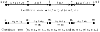
Figure 4: The $5$-vertex certificate graph for associativity. Both pictures represent the same graph certificate $H$, where the second one has been labelled according to the notations of our abstract language.

We use the algorithmic framework of Theorem 8 to load the graph $H$. Let $r_{1}=n/10,r_{2}=n^{4/7},r_{3}=n^{6/7},r_{4}=n^{5/7},r_{5}=1$ and $d_{21}=n^{6/7},d_{23}=n^{6/7},d_{34}=n^{5/7},d_{54}=1$. Here $d_{ij}$ indicates the average degree of vertices in the smaller of $A_{i},A_{j}$ for edges directed from $A_{i}$ to $A_{j}$. It can be checked that this is an admissible set of parameters. Note that as $r_{5}d_{54}<<r_{4}$, loading $a_{5}\circ a_{4}$ will be done in the sparse regime. We use the loading schedule $S=[1,2,4,3,(2,1),(2,3),(3,4),5,(5,4)]$. The setup cost becomes $r_{2}d_{21}+r_{2}d_{23}+r_{4}d_{34}+r_{5}d_{54}=n^{10/7}$, and the costs of loading the vertices and edges are all bounded by $n^{10/7}$ as given in the following tables.

Stage	load $a_{1}$	load $a_{2}$	load $a_{4}$	load $a_{3}$
Global cost	$\sqrt{{n}/{r_{1}}}$	$\sqrt{{n}/{r_{2}}}$	$\sqrt{{n}/{r_{4}}}$	$\sqrt{{n}/{r_{3}}}$
Local cost	$\sqrt{n}{r_{2}}d_{21}/{r_{1}}$	$\sqrt{n}(d_{21}+d_{23})$	$\sqrt{n}(d_{34}+r_{5}d_{54}/r_{4})$	$\sqrt{n}(r_{4}d_{34}/r_{3}+r_{2}d_{23}/r_{3})$
Cost	$\sqrt{n}r_{2}d_{21}/r_{1}$	$\frac{n}{\sqrt{r_{1}}}(d_{21}+d_{23})$	$\frac{n^{3/2}}{\sqrt{r_{1}r_{2}}}(d_{34}+r_{5}d_{54}/r_{4})$	$\frac{n^{2}}{\sqrt{r_{1}r_{2}r_{4}}}(r_{4}d_{34}/r_{3}+r_{2}d_{23}/r_{3})$
Value	$n^{13/14}$	$n^{19/14}$	$n^{10/7}$	$n^{10/7}$

Stage	load $a_{2}\circ a_{1}$	load $a_{2}\circ a_{3}$	load $a_{3}\circ a_{4}$
Global cost	$\sqrt{r_{1}/d_{21}}$	$\sqrt{r_{3}/d_{23}}$	$\sqrt{r_{3}/d_{34}}$
Local cost	${r_{1}}$	${r_{3}}$	${r_{3}}$
Cost	$\frac{n^{2}}{\sqrt{r_{2}r_{3}r_{4}}}\sqrt{r_{1}}$	$\frac{n^{2}}{\sqrt{r_{2}r_{4}d_{21}}}\sqrt{r_{1}r_{3}}$	$\frac{n^{2}}{\sqrt{r_{2}r_{4}d_{21}d_{23}}}r_{3}$
Value	$n^{10/7}$	$n^{19/14}$	$n^{19/14}$

Stage	load $a_{5}$	load $a_{5}\circ a_{4}$
Global cost	$\sqrt{n/r_{5}}$
Local cost	$\sqrt{n}d_{54}$	$\sqrt{r_{4}r_{5}}$
Cost	$\frac{n^{5/2}}{\sqrt{r_{2}r_{4}d_{21}d_{23}d_{34}}}\sqrt{r_{3}}d_{54}$	$\frac{n^{5/2}}{\sqrt{r_{2}d_{21}d_{23}d_{34}}}\sqrt{r_{3}}$
Value	$n^{15/14}$	$n^{10/7}$

∎

The algorithms for finding $k$-vertex subgraphs given in [13, 9] have complexity $O(n^{1.48})$ for finding a $4$-path, but it was not realized there that these algorithms apply to a much broader class of functions like associativity. The key property that is used for this application is that in the basic learning graph model the complexity depends only on the index sets of $1$-certificates and not on the underlying alphabet. This property was previously observed by Mario Szegedy in the context of limitations of the basic learning graph model [8]. He observed that the basic learning graph complexity of the threshold-$2$ function is $\Theta(n^{2/3})$, rather than the true value $\Theta(\sqrt{n})$, as threshold-2 and element distinctness have the same $1$-certificate index sets.

References

- [1] A. Belovs. Learning-graph-based quantum algorithm for k-distinctness. In Prooceedings of 53rd Annual IEEE Symposium on Foundations of Computer Science, 2012.
- [2] A. Belovs. Span programs for functions with constant-sized 1-certificates. In Proceedings of 44th Symposium on Theory of Computing Conference, pages 77–84, 2012.
- [3] A. Belovs and T. Lee. Quantum algorithm for k-distinctness with prior knowledge on the input. Technical Report arXiv:1108.3022, arXiv, 2011.
- [4] S. Dörn and T. Thierauf. The quantum complexity of group testing. In Proceedings of the 34th conference on current trends in theory and practice of computer science, pages 506–518, 2008.
- [5] Lov K. Grover. A fast quantum mechanical algorithm for database search. In Proceedings of 28th ACM Symposium on the Theory of Computing, pages 212–219, 1996.
- [6] P. Høyer and R. Špalek. Lower bounds on quantum query complexity. Bulletin of the European Association for Theoretical Computer Science, 87, 2005. Also arXiv report quant-ph/0509153v1.
- [7] Peter Høyer, Troy Lee, and Robert Špalek. Negative weights make adversaries stronger. In Proceedings of 39th ACM Symposium on Theory of Computing, pages 526–535, 2007.
- [8] R. Kothari. Personal Communication, 2011.
- [9] T. Lee, F. Magniez, and M. Santha. A learning graph based quantum query algorithm for finding constant-size subgraphs. Technical Report arXiv:1109.5135, arXiv, 2011.
- [10] F. Magniez, M. Santha, and M. Szegedy. Quantum algorithms for the triangle problem. SIAM Journal on Computing, 37(2):413–424, 2007.
- [11] Ben W. Reichardt. Reflections for quantum query algorithms. In Proceedings of 22nd ACM-SIAM Symposium on Discrete Algorithms, pages 560–569, 2011.
- [12] P. Shor. Algorithms for quantum computation: Discrete logarithm and factoring. SIAM Journal on Computing, 26(5):1484–1509, 1997.
- [13] Y. Zhu. Quantum query complexity of subgraph containment with constant-sized certificates. Technical Report arXiv:1109.4165v1, arXiv, 2011.