Properties of Z=120 nuclei and the $\alpha$-decay chains of the ^292,304120 isotopes using relativistic and non-relativistic formalisms

Abstract

The ground state and first intrinsic excited state of superheavy nuclei with Z=120 and N=160-204 are investigated using both non-relativistic Skyrme-Hartree-Fock and the axially deformed Relativistic Mean Field formalisms. We employ a simple BCS pairing approach for calculating the energy contribution from pairing interaction. The results for isotopic chain of binding energy, quadrupole deformation parameter, two neutron separation energies and some other observables are compared with the FRDM and some recent macroscopic-microscopic calculations. We predict superdeformed ground state solutions for almost all the isotopes. Considering the possibility of magic neutron number, two different mode of $\alpha$-decay chains ²⁹²120 and ³⁰⁴120 are also studied within these frameworks. The $Q_{\alpha}$-values and the half-life $T_{1/2}^{\alpha}$ for these two different mode of decay chains are compared with FRDM and recent macroscopic-microscopic calculations. The calculation is extended for the $\alpha$-decay chains of ²⁹²120 and ³⁰⁴120 from their exited state configuration to respective configuration, which predicts long half-life $T_{1/2}^{\alpha}$(sec.).

1 Introduction

By superheavy elements (SHEs) we mean elements with proton number (Z) near the next magic number beyond the magic number Z = 82, corresponding to Pb. The possibility of finding the magic or doubly magic isotopes of SHEs led to the prediction of a region of enhanced stability in the 1960’s [1, 2, 3, 4, 5]. Since then,the nuclear synthesis and investigation of new superheavy elements has been a challenging problem in nuclear physics. A worldwide effort has been made to explore the island of stability of SHEs. Many experimental groups in various laboratories are trying hard to study various peculiar aspects of SHEs [6, 7, 8, 9, 10, 11, 12, 13, 14, 15, 16, 17]. For the synthesis of heavy and superheavy elements, two approaches have been successfully employed. Firstly, via cold fusion reactions, which have been successfully used to synthesize superheavy elements up to Z = 112 at GSI [7, 18, 19, 20, 21] and that with Z = 113 at RIKEN [22], and to confirm these experiments at RIKEN [22, 23, 24] and LBNL [25]. Secondly, hot fusion reactions have also been used to synthesize superheavy elements from Z = 112 to 116 and 118 [26, 27, 28, 29, 30, 31]. Efforts are on to synthesize still heavier elements in various laboratories all over the world.

An impressive progress in the synthesis and experimental studies of the heaviest nuclei [6, 7, 8, 9, 10, 11, 12, 13, 14, 15, 16, 17] requires intensive theoretical studies of them. Their studies are needed for predicting stability properties of as yet undiscovered SHEs and also for the interpretation of already existing experimental results. In the last decade, several theoretical investigations of SHEs are focused both on the structure and decay properties and on the synthesis mechanism [32, 33, 34, 35, 36, 37, 38, 39, 40, 41, 42, 43, 44, 45, 46, 47, 48, 49, 50, 51, 52, 53, 54, 55, 56, 57, 58, 59, 60, 61].

In general most of the advanced model calculations predict the existence of a closed shell at N = 184; however, they differ in predicting the atomic number of the closed proton shell. Some macroscopic-microscopic (MM) theories which traditionally involve a priory the knowledge of densities, single particle potentials and other bulk properties, they predict the magic shells at Z=114 and N=184 [32, 33, 34, 5, 35]. At the same time, the predictions of shell closure for the superheavy region within the relativistic and non-relativistic theories depend mostly on the force parameters [36, 37]. For example, the Skyrme Hartree-Fock (SHF) calculation with SkI4 force gives Z=114, N=184 as the next shell-closures and the relativistic microscopic mean field formalism (RMF) [38] predicts the probable shell-closures at Z=120 and N=184. Recently, more microscopic theoretical calculations have predicted the various other region of stability, beyond Z=82, N=126, as Z=120, N=172 or 184 [36, 38, 39] and Z=124 or 126, N=184 [41, 42, 43]. Such estimations of structure properties of nuclei in the superheavy mass region is a challenging area in nuclear physics and a fruitful path towards the understanding of ’island of stability’ beyond the spherical doubly-magic nucleus [62, 63]. Progress in understanding the structure of the heaviest nuclei can be achieved through the theoretical and experimental studies of production and decay of superheavy elements (SHEs).

SHEs are an excellent testing ground for nuclear theory models. The SHE in the ground state is formed at the end of the cooling-down process of the compound nucleus. The $\alpha$ particles are mainly emitted from the ground state of a formed SHE, because as a rule, the $\gamma$-decay half-lives of low-lying excitation states are shorter than the $\alpha$-decay half-lives of corresponding levels. Alpha decay is one of two main decay modes of the heaviest nuclei. It is important for these nuclei because: many of the already known heavy nuclei decay by this mode, also many of the nuclei not yet observed, specially superheavy nuclei are predicted to be $\alpha$ emitters, and properties of this decay give a good method for identification of decaying nuclei (genetic chain). The amount of already collected data for $\alpha$-decay is quite large [7, 17, 13, 14, 9, 8, 6, 15, 16, 10, 11, 12, 18, 19, 20, 21, 22, 23, 24, 25, 26, 27, 28, 29, 30, 31, 64, 65, 66] and is still increasing. It is important then, both the interpretation of existing data and for predictions for new experiments, to realize with what accuracy one can presently describe both observables of this process: $\alpha$-decay energy $Q_{\alpha}$ and $\alpha$-decay half life $T_{\alpha}$. The $Q_{\alpha}$ energy is obtained from masses of the respective nuclei, which are presently described by a number of various methods [32, 33, 35, 36, 38, 39, 42, 43, 45, 46, 47, 48, 49, 51, 52, 54, 55, 56, 59, 60, 61, 67, 68, 69, 70, 71, 72, 73, 74, 75, 76, 77]. Half-lives $T_{1/2}^{\alpha}$ are usually described in a phenomenological way. The very possibility of an extremely heavy Z nucleus motivated us to see the structure of such nuclei in an isotopic mass chain. Therefore, on the basis of the RMF and nonrelativistic SHF methods, we calculated the bulk properties of a Z = 120 nucleus in an isotopic chain of mass A = 280-324. This choice of mass range covers both the predicted neutron magic numbers N = 172 and 184.

The paper is organized as follows. Section II gives a brief description of the relativistic and nonrelativistic mean-field formalism. The pairing effects for open shell nuclei, included in our calculations, are also discussed in this section. The results of our calculation are presented in Section III, and Section IV includes the $\alpha$-decay modes of ²⁹²120 and ³⁰⁴⁴120 isotopes. A summary of our results, together with the concluding remarks, are given in the last Section V.

2 Theoretical Framework

2.1 The Skyrme Hartree-Fock Method

The general form of the Skyrme effective interaction, used in the mean-filed models, can be expressed as an energy density functional $\mathcal{H}$ [78, 79, 80],

$$\mathcal{H}=\mathcal{K}+\mathcal{H}_{0}+\mathcal{H}_{3}+\mathcal{H}_{eff}+....,$$ (1)

where $\mathcal{K}=\frac{\hbar^{2}}{2m}\tau$ is the kinetic energy term with $m$ as the nucleon mass, $\mathcal{H}_{0}$ is the zero range, $\mathcal{H}_{3}$ the density dependent term, and $\mathcal{H}_{eff}$ the effective-mass dependent term, relevant for calculating the properties of nuclear matter, are functions of nine parameters, $t_{i}$, $x_{i}$ (i = 0, 1, 2, 3), and $\eta$, given as

$$\mathcal{H}_{0} = \frac{1}{4}t_{0}\left[\left(2+x_{0}\right)\rho^{2}-\left(2x_{0}+1\right)\left(\rho_{p}^{2}+\rho_{n}^{2}\right)\right]$$ (2)

$$\mathcal{H}_{3} = \frac{1}{24}t_{3}\rho^{\eta}\left[\left(2+x_{3}\right)\rho^{2}-\left(2x_{3}+1\right)\left(\rho_{p}^{2}+\rho_{n}^{2}\right)\right]$$ (3)

$$\mathcal{H}_{eff} = \frac{1}{8}\left[t_{1}\left(2+x_{1}\right)+t_{2}\left(2+x_{2}\right)\right]\tau\rho$$ (4)

$$+ \frac{1}{8}\left[t_{2}\left(2x_{2}+1\right)-t_{1}\left(2x_{1}+1\right)\right]\left(\tau_{p}\rho_{n}+\tau_{n}\rho_{p}\right).$$

The other terms, representing the surface contributions of a finite nucleus with $b_{4}$ and $b_{4}^{\prime}$ as additional parameters, are

$$\mathcal{H}_{S\rho} = \frac{1}{16}\left[3t_{1}\left(1+\frac{1}{2}x_{1}\right)-t_{2}\left(1+\frac{1}{2}x_{2}\right)\right]\left(\vec{\nabla}\rho\right)^{2}$$ (5)

$$-\frac{1}{16}\left[3t_{1}\left(x_{1}+\frac{1}{2}\right)+t_{2}\left(x_{2}+\frac{1}{2}\right)\right]$$

$$\times\left[\left(\vec{\nabla}\rho_{n}\right)^{2}+\left(\vec{\nabla}\rho_{p}\right)^{2}\right],$$

and

$$\mathcal{H}_{S\vec{J}}=-\frac{1}{2}\left[b_{4}\rho\vec{\nabla}\cdot\vec{J}+b_{4}^{\prime}\left(\rho_{n}\vec{\nabla}\cdot\vec{J_{n}}+\rho_{p}\vec{\nabla}\cdot\vec{J_{p}}\right)\right],$$ (6)

here, the total nucleon number density $\rho=\rho_{n}+\rho_{p}$, the kinetic energy density $\tau=\tau_{n}+\tau_{p}$, and the spin-orbit density $\vec{J}=\vec{J_{n}}+\vec{J_{p}}$, with $n$ and $p$ referring to neutron and proton, respectively. The $\vec{J_{q}}=0$, $q=n$ or $p$, for spin-saturated nuclei, i.e., for nuclei with major oscillator shells completely filled. The total binding energy (BE) of a nucleus is the integral of the energy density functional $\mathcal{H}$. We have used here the Skyrme SkI4 and SLy4 sets with $b_{4}\neq b_{4}^{\prime}$ [81], designed for considerations of proper spin-orbit interaction in finite nuclei, related to the isotopic shifts in the Pb region.

2.2 The Relativistic Mean-Field Formalism

The relativistic Lagrangian density for a nucleon-meson many-body system [82, 83, 84, 85],

$${\cal L} = \overline{\psi_{i}}\{i\gamma^{\mu}\partial_{\mu}-M\}\psi_{i}+{\frac{1}{2}}\partial^{\mu}\sigma\partial_{\mu}\sigma-{\frac{1}{2}}m_{\sigma}^{2}\sigma^{2}$$ (7)

$$-{\frac{1}{3}}g_{2}\sigma^{3}-{\frac{1}{4}}g_{3}\sigma^{4}-g_{s}\overline{\psi_{i}}\psi_{i}\sigma-{\frac{1}{4}}\Omega^{\mu\nu}\Omega_{\mu\nu}$$

$$+{\frac{1}{2}}m_{w}^{2}V^{\mu}V_{\mu}+{\frac{1}{4}}c_{3}(V_{\mu}V^{\mu})^{2}-g_{w}\overline{\psi}_{i}\gamma^{\mu}\psi_{i}V_{\mu}$$

$$-{\frac{1}{4}}\vec{B}^{\mu\nu}.\vec{B}_{\mu\nu}+{\frac{1}{2}}m_{\rho}^{2}{\vec{R}^{\mu}}.{\vec{R}_{\mu}}-g_{\rho}\overline{\psi}_{i}\gamma^{\mu}\vec{\tau}\psi_{i}.\vec{R^{\mu}}$$

$$-{\frac{1}{4}}F^{\mu\nu}F_{\mu\nu}-e\overline{\psi}_{i}\gamma^{\mu}\frac{\left(1-\tau_{3i}\right)}{2}\psi_{i}A_{\mu}.$$

All the quantities have their usual well-known meanings. From the above Lagrangian we obtain the field equations for the nucleons and mesons. These equations are solved by expanding the upper and lower components of the Dirac spinors and the boson fields in an axially deformed harmonic oscillator basis, with an initial deformation $\beta_{0}$. The set of coupled equations is solved numerically by a self-consistent iteration method. The center-of-mass motion energy correction is estimated by the usual harmonic oscillator formula $E_{c.m.}=\frac{3}{4}(41A^{-1/3})$. The quadrupole deformation parameter $\beta_{2}$ is evaluated from the resulting proton and neutron quadrupole moments, as $Q=Q_{n}+Q_{p}=\sqrt{\frac{16\pi}{5}}(\frac{3}{4\pi}AR^{2}\beta_{2})$. The root mean square (rms) matter radius is defined as $\langle r_{m}^{2}\rangle={1\over{A}}\int\rho(r_{\perp},z)r^{2}d\tau$, where $A$ is the mass number, and $\rho(r_{\perp},z)$ is the deformed density. The total binding energy and other observables are also obtained by using the standard relations, given in [83, 84]. We have used the recently proposed parameter set NL3* [86], which improves the description of the ground state properties of many nuclei over parameter set NL3 [87], and simultaneously provides an excellent description of excited states with collective character in spherical as well as in deformed nuclei. Just to compare, we have also used the parameter set NL3 [87], which has been used in the last ten years with great success to describe many ground state properties of finite nuclei all over the periodic table [88, 89, 90, 91, 92, 93, 94, 95]. However, in the mean time, several other relativistic mean-field interactions have been developed. In particular, the density dependent meson-exchange DD-ME1 [96] and DD-ME2 [97] effective interactions. These effective interactions have been adjusted to improve the isovector channel, which has been the weak point of the NL3 [87] effective interaction, and provide a very successful description of different aspects of finite nuclei [98, 99]. Recently, a new DD-PC1 [100] (density dependent point coupling) effective interaction has been developed, which works very well in the region of deformed heavy nuclei. As outputs, we obtain different potentials, densities, single-particle energy levels, radii, deformations and the binding energies. For a given nucleus, the maximum binding energy corresponds to the ground state and other solutions are obtained as various excited intrinsic states.

2.3 Pairing Calculation

It is well know that pairing correlations have to be included in any realistic calculation of medium and heavy nuclei. In principle, the microscopic Hartree-Fock-Bogoliubov (HFB) theory should be used, which have been discussed in several articles [98, 99, 100, 101, 102, 103, 104, 105] and in the references given there. However, for pairing calculations of a broad range of nuclei not too far from the $\beta$-stability line, a simpler approach, the constant gap, BCS-pairing approach is reasonably well. But, this simple approach breaks down for nuclei far from the valley of $\beta$-stability, where the coupling to the continuum is important [106]. In the present study, we treat the pairing correlations using the BCS approach. Although the BCS approach may fail for light neutron rich nuclei, the nuclei considered here are not light neutron rich nuclei and the RMF results with BCS treatment should be reliable.

The contribution of the pairing interaction to the total energy, for each nucleon, is

$$E_{pair}=-G\left[\sum_{i>0}u_{i}v_{i}\right]^{2}$$ (8)

where $v_{i}^{2}$ and $u_{i}^{2}=1-v_{i}^{2}$ are the occupation probabilities, and $G$ is the pairing force constant [83, 107, 108]. The variational procedure with respect to the occupation numbers $v_{i}^{2}$, gives the BCS equation

$$2\epsilon_{i}u_{i}v_{i}-\triangle(u_{i}^{2}-v_{i}^{2})=0$$ (9)

and the gap $\Delta$ is defined by

$$\triangle=G\sum_{i>0}u_{i}v_{i}$$ (10)

This is the famous BCS equation for pairing energy. The densities are contained within the occupation number

$$n_{i}=v_{i}^{2}=\frac{1}{2}\left[1-\frac{\epsilon_{i}-\lambda}{\sqrt{(\epsilon_{i}-\lambda)^{2}+\triangle^{2}}}\right]$$ (11)

For the pairing gaps for proton and neutron, we choose the standard expressions, which are valid for nuclei both on or away from the stability line, and are given by the expressions [109, 110]:

$$\triangle_{p} = RB_{s}e^{sI-tI^{2}}/Z^{1/3}\;\;\;\;\;\mbox{and}$$ (12)

$$\triangle_{n} = RB_{s}e^{-sI-tI^{2}}/A^{1/3}$$ (13)

The inputs of pairing gaps i.e., $R$ = 5.72, $s$ = 0.118, $t$ = 8.12, $B_{s}$ = 1, and $I=(N-Z)/(N+Z)$ are used in nuclear physics for many years. We consider that it is suitable here. The occupation probability is calculated using Eqs. (12) and (13), and the chemical potentials $\lambda_{n}$ and $\lambda_{p}$ are determined by the particle numbers for protons and neutrons. Using Eqs. (10) and (11) the pairing energy for nucleon can be written as

$$E_{pair}=-\frac{\Delta^{2}}{G}=-\triangle\sum_{i>0}u_{i}v_{i}$$ (14)

It can be seen from Eq. (14), that in the present approach to include the pairing effects using the constant pairing gap, the pairing energy $E_{pair}$ is not constant since it depends on the occupation probabilities $v_{i}^{2}$ and $u_{i}^{2}$, and hence on the deformation parameter $\beta_{2}$, particularly near the Fermi surface. It is known to us that the pairing energy $E_{pair}$ diverges if it is extended to an infinite configuration space for a constant pairing parameter $\triangle$ and force constant $G$. Also, for the states spherical or deformed, with large momenta near the Fermi surface, $\triangle$ decreases in all the realistic calculations with finite range forces. However, for the sake of simplicity of the calculation, we have taken constant pairing gap by assuming that the pairing gap for all states are equal to each other near the Fermi surface. In the present calculations we have used a pairing window, and all the equations extended up to the level $\epsilon_{i}-\lambda\leq 2(41A^{1/3})$, where a factor of 2 has been included in order to reproduce the pairing correlation energy for neutrons in ¹¹⁸Sn using Gogny force [107]. This kind of approach to treat the pairing correlation, has already been used by us and many other authors in RMF model as well in non relativistic SHF model [47, 83, 107, 111, 112, 113, 114].

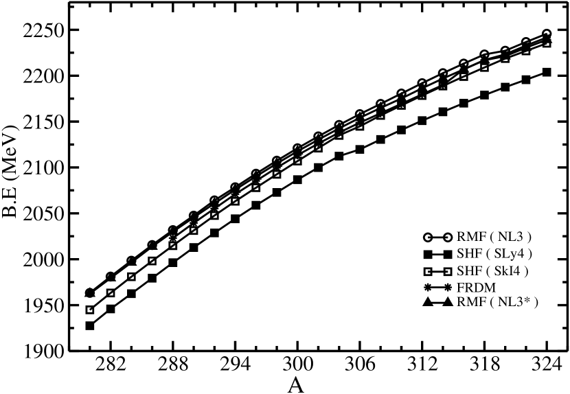
Figure 1: The total binding energy BE for ^280-324120 nuclei in RMF(NL3*), RMF(NL3), SHF(SkI4) and SHF(SLy4) calculations compared with the FRDM results [62] wherever available.

3 Results and Discussion

3.1 Ground state properties using the SHF and RMF models

There exist a number of parameter sets for solving the standard SHF Hamiltonians and RMF Lagrangians. In many of our previous works and those of other [39, 83, 87, 115, 116, 117] the ground state properties, like the binding energies (BE), quadrupole deformation parameters $\beta_{2}$, charge radii ($r_{c}$), and other bulk properties , are evaluated by using the various nonrelativistic and relativistic parameter sets. It is found that, more or less, most of the recent parameter sets reproduce well the ground state properties, not only of stable normal nuclei but also of exotic nuclei far away from the valley of $\beta$-stability. This means that if one uses a reasonably acceptable parameter set, the predictions of the model will remain nearly force independent. In this paper we have used the improved version of NL3 parameter set (NL3*), standard NL3, SkI4 and SLy4 parameter sets for our calculations.

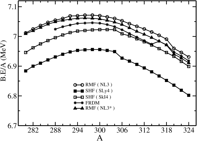
Figure 2: The binding energy per particle BE/A for the superheavy isotopes ^280-324120 obtained in RMF(NL3*), RMF(NL3), SHF(SkI4) and SHF(SLy4) formalism compared with the FRDM results [62] wherever available.

3.2 Binding Energy and Two-neutron Separation Energy and Pairing Energy

Binding energies are important quantities of nuclei and they are directly related to the stability of nuclei and to $\alpha$-decay energies. Whether a model can quantitatively reproduce the experimental binding energy is a crucial criterion to judge the validity of the model for superheavy nuclei. Figure 1 shows the total binding energy BE, obtained in both nonrelativistic SHF and relativistic RMF formalism compared with the Finite Range Droplet Model (FRDM) results [67, 68]. From the figure it is clear that, the binding energy obtained in both the RMF and SHF models are qualitatively similar. We notice that the binding energy, obtained using the NL3 and NL3* parameter set are almost equal within lower mass region but, towards higher mass region, the binding energy using NL3* parameter set, is gradually getting lower values than NL3 parameter set, which are over-estimate to both the SHF (SkI4) and SHF (SLy4) results by almost a constant factor. For the total binding energy of the isotopic chain in Tables 1, 2 and Figure 1, we notice that the macro-microscopic FRDM calculation lies in between microscopic RMF and SHF. In case of SHF (SkI4) the difference decreases gradually towards the higher mass region.

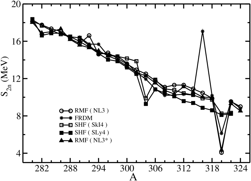
Figure 3: The two-neutron separation energy $S_{2n}$ for ^280-324120 nuclei, obtained from RMF(NL3*), RMF(NL3), SHF(SkI4) and SHF(SLy4) formalisms and compared with the FRDM results [62] wherever available.

The binding energy per particle (BE/A) for the isotopic chain is also plotted in Figure 2. We notice that the SHF and RMF curves could almost be overlapped with one another through a constant scaling factor. The FRDM calculation lies in between RMF and SHF. This means, qualitatively, all the curves show a similar behavior. In general, the BE/A value starts increasing with the increase of mass number A, reaching a peak value at A $\sim$ 304 for RMF, SHF and FRDM models. This means that ${}^{304}120$ is the most stable element from the binding energy point of view, which is situated at A$\sim$ 304 (N=184, Z=120). Interestingly, this neutron number are close to N = 184, which is the next predicted magic number [118]. It is worthy to mention that, the results obtained in the present calculation are almost consistents to the prediction by earlier calculations [36, 37, 50, 51, 52, 53, 54] using some different force parameters. Hence, we may note that the results for binding energy and related observables like magic numbers are independent of force parameters.

In Tables 1 and 2, we also show a comparison of the calculated two-neutron separation energy $S_{2n}$(N,Z) = BE(N,Z)-BE(N-2,Z) with the Finite Range Droplet Model (FRDM) predictions of Ref. [67, 68], wherever possible. From the tables, we find that the microscopic $S_{2n}$ values agree well with the macro-microscopic FRDM calculations. The comparisons of $S_{2n}$ for RMF and SHF models with the FRDM result are further shown in Figure 3, which clearly shows that the RMF and the FRDM $S_{2n}$ values coincide remarkably well, except at mass A = 316 which seems spurious due to some error somewhere in the case of FRDM. Apparently, the $S_{2n}$ decrease gradually with increase of neutron number, except for the noticeable kinks at A = 282 (N = 172) and 318 (N = 198) in RMF(NL3*), at A = 292 (N = 172) and 318 (N = 198) in RMF(NL3), at A = 294 (N = 174) and 318 (N = 198) in FRDM, at A = 282 (N = 162) and 304 (N = 184) in SHF (SLy4) and at A = 304 (N = 184) and 318 (N = 198) in SHF (SkI4). Interestingly, these neutron numbers are close to either N = 172 or 184 magic numbers.

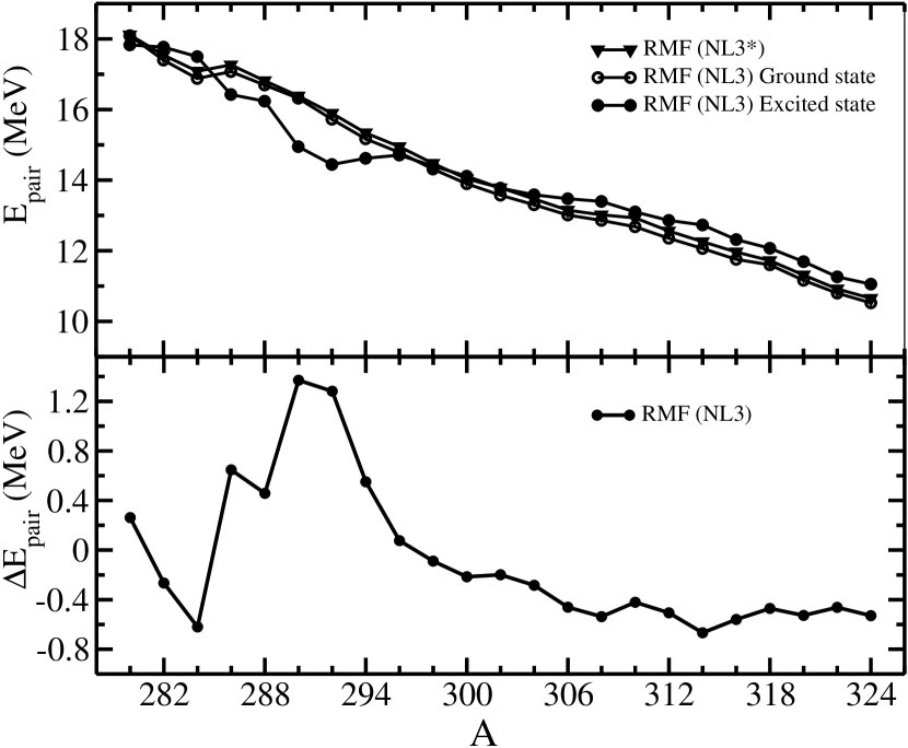
Figure 4: (a) The Pairing energy $E_{pair}$ for the ground state and first excited states and (b) the pairing energy difference $\Delta E_{pair}$ between the $E_{pair}$ values of ground and first excited states [$\Delta E_{pair}$ = $E_{pair}$(g.s.) - $E_{pair}$(e.s.)] for ^280-324120 nuclei as a function of mass number, using the RMF formalism with NL3* and NL3 parameter set.

Figure 4, show the pairing energy $E_{pair}$ as well as the pairing energy difference $\Delta E_{pair}$ as a function of mass number A. In Figure 4(a), we show the pairing energy $E_{pair}$ for both the ground state (g.s.) using RMF(NL3*) and RMF(NL3), and the first excited state (e.s.) using RMF(NL3), referring to different $\beta_{2}$ values for the full isotopic chain. The difference in the two $E_{pair}$ values, i.e. $\Delta E_{pair}$ = $E_{pair}$(g.s.) - $E_{pair}$(e.s.), is shown in Figure 4(b). It is clear from Figure 4(a) that $E_{pair}$ decreases with an increase in mass number A; i.e., even if the $\beta_{2}$ values for two nuclei are the same, the pairing energies are different from one another. From the above results, it can be seen that for a given nucleus, pairing energy $E_{pair}$ depends only marginally on the quadrupole deformation $\beta_{2}$. On the other hand, even if the $\beta_{2}$ values for two nuclei are same, the $E_{pair}$ values are different from one another, depending on the filling of the nucleons.

3.3 Shape coexistence

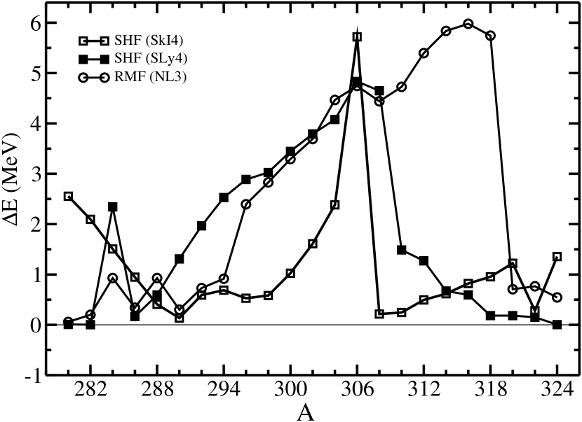
Figure 5: The energy difference between the ground state and the first excited state in both nonrelativistic SHF(SkI4), SHF(SLy4) and RMF formalisms with NL3* and NL3 parameter set.

We have also calculated the existing other solutions for the whole Z = 120 isotopic chain, both in prolate and oblate deformed configurations. In many cases, we find low-lying excited states. As a measure of the energy difference between the ground band and the first excited state, we have plotted in Figure 5 the binding energy difference $\triangle E$ between the two solutions, noting that the maximum binding energy solution refers to the ground state (g.s.) and all other solutions to the intrinsic excited states (e.s.). From Figure 5, we notice that, in RMF calculations, the energy difference $\triangle E$ is small for neutron-deficient isotopes, but it increases with increase of mass number A in the isotopic series. This small difference in the binding energy for neutron-deficient isotopes is an indication of shape coexistence. In other words, the two solutions in these nuclei are almost degenerate for a small difference of output in energy. For example, in ²⁹⁰120, the two solutions for $\beta_{2}$ = 0.555 and $\beta_{2}$ = 0.002 are completely degenerate with binding energies of 2047.503 and 2047.202 MeV. This later result suggests that the ground state can be changed to the excited state and vice-versa by a small change in the input, like the pairing strength, etc., in the calculations. Similarly, in case of SHF (SkI4) calculation, the energy difference $\triangle E$ remains small between mass number A = 286 to 300 and between mass number A = 308 to 324, indicating of the presence of shape coexistence. We also have the indication of the presence of shape coexistence through SHF (SLy4) calculation. In any case, such a phenomenon is known to exist in many other regions of the periodic table [119, 120, 121, 122].

Table 1: The RMF(NL3*), RMF(NL3), SHF (SkI4) and SHF (SLy4) results for binding energy BE, the quadrupole deformation parameter $\beta_{2}$, two-neutron separation energy $S_{2n}$ and the binding energy difference $\triangle E$ between the ground- and first-exited state solutions, compared with the corresponding Finite Range Droplet Model (FRDM) results [62] for the isotopic chain of ^280-302120. The energy is in MeV.

Nucleus	Formalism	BE	$\beta_{2}$	$S_{2n}$	$\Delta E$
280	RMF (NL3)	1963.33	0.258	18.11	0.058
	RMF (NL3*)	1962.54	0.258	18.02
	SHF (SkI4)	1944.92	0.529	18.32	2.555
	SHF (SLy4)	1927.51	0.227	18.37	0.008
282	RMF (NL3)	1981.08	-0.422	17.75	0.200
	RMF (NL3*)	1979.43	-0.426	16.89
	SHF (SkI4)	1963.24	0.520	17.68	2.096
	SHF (SLy4)	1945.88	0.227	16.62	0.003
284	RMF (NL3)	1998.42	-0.428	17.34	0.929
	RMF (NL3*)	1996.46	-0.432	17.03
	SHF (SkI4)	1980.91	0.519	17.16	1.507
	SHF (SLy4)	1962.51	0.202	16.86	2.343
286	RMF (NL3)	2015.48	0.567	17.16	0.340
	RMF (NL3*)	2013.78	0.567	17.32
	SHF (SkI4)	1998.08	0.521	16.76	0.947
	SHF (SLy4)	1979.37	0.537	16.86	0.165
288	RMF (NL3)	2031.75	0.560	16.28	0.929
	RMF (NL3*)	2029.97	0.562	16.19
	SHF (SkI4)	2014.83	0.523	16.48	0.408
	SHF (SLy4)	1996.23	0.122	16.51	0.593
	FRDM	2023.03	-0.113
290	RMF (NL3)	2047.50	0.551	15.75	0.301
	RMF (NL3*)	2045.56	0.556	15.59
	SHF (SkI4)	2031.31	0.119	16.37	0.135
	SHF (SLy4)	2012.74	0.115	15.98	1.310
	FRDM	2039.49
292	RMF (NL3)	2064.11	0.540	16.61	0.730
	RMF (NL3*)	2060.87	0.547	15.31
	SHF (SkI4)	2047.68	0.113	15.53	0.591
	SHF (SLy4)	2028.71	0.107	15.38	1.966
	FRDM	2055.19	-0.130	15.70
294	RMF (NL3)	2078.43	0.536	14.61	0.916
	RMF (NL3*)	2075.85	0.541	14.98
	SHF (SkI4)	2063.21	0.110	14.75	0.688
	SHF (SLy4)	2044.09	0.097	14.69	2.528
	FRDM	2070.87	0.081	15.68
296	RMF (NL3)	2093.19	0.542	14.76	2.394
	RMF (NL3*)	2090.29	0.545	14.44
	SHF (SkI4)	2077.96	0.087	14.59	0.529
	SHF (SLy4)	2058.78	0.088	14.03	2.887
	FRDM	2085.32	-0.096	14.45
298	RMF (NL3)	2107.35	0.551	14.16	0.058
	RMF (NL3*)	2104.30	0.554	14.01
	SHF (SkI4)	2092.55	0.066	14.38	0.583
	SHF (SLy4)	2072.81	0.060	13.86	3.026
	FRDM	2099.73	-0.079	14.41
300	RMF (NL3)	2120.92	0.561	13.57	3.292
	RMF (NL3*)	2117.63	0.564	13.33
	SHF (SkI4)	2106.94	0.045	14.16	1.026
	SHF (SLy4)	2086.68	0.040	13.19	3.446
	FRDM	2113.39	-0.008	13.66
302	RMF (NL3)	2133.86	0.579	12.94	3.691
	RMF (NL3*)	2130.28	0.586	12.65
	SHF (SkI4)	2121.09	0.024	13.86	1.611
	SHF (SLy4)	2099.87	0.019	12.5	3.791
	FRDM	2126.05	0.000	12.66

3.4 Quadrupole deformation parameter

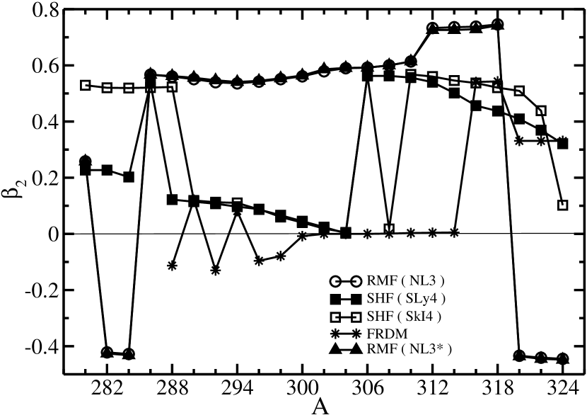
Figure 6: Comparison of quadrupole deformation parameter obtained from nonrelativistic SHF(SkI4), SHF(SLy4) and relativistic mean-field formalism (RMF) with NL3* and NL3 parameter set, compared with the FRDM results [62] wherever available.

The quadrupole deformation parameter $\beta_{2}$, for both the ground and first excited states, is also determined within the two formalisms. In some of the earlier RMF and SHF calculations, it was shown that the quadrupole moment obtained from these theories reproduce the experimental data pretty well [39, 78, 79, 82, 83, 87, 115, 123, 124]. The ground state (g.s.) quadrupole deformation parameter $\beta_{2}$ values plotted in Figure 6 for SHF and RMF formalisms, and compared with the FRDM results [67, 68] show that the FRDM results differ strongly along the whole mass regions. In both the SHF (SkI4) and SHF (SLy4) results, we find that the solutions for the whole isotopic chain are prolate. However, in some mass region, we find highly deformed prolate solutions in the ground state configuration. In RMF formalism using both NL3* and NL3 parameter set, we find shape change from prolate to highly deformed oblate at A = 282. Then, with increase in mass number there is a shape change from highly oblate to highly prolate, and again we find a shape change from highly prolate to highly oblate at A = 320. A more careful inspection show that the solutions for the whole isotopic chain are prolate, except at A = 282, 284 and at A = 320-324 for both the RMF(NL3*) and RMF(NL3) model. Interestingly, most of the isotopes are superdeformed in their ground state configurations, and because of the shape coexistence properties of these isotopes, sometimes it is possible that the ground state could be the near spherical solution.

Table 2: Same as TABLE I, for the isotopic chain of ^304-324120.

Nucleus	Formalism	BE	$\beta_{2}$	$S_{2n}$	$\Delta E$
304	RMF (NL3)	2146.37	0.590	12.51	4.466
	RMF (NL3*)	2142.57	0.591	12.29
	SHF (SkI4)	2134.96	0.002	9.89	2.383
	SHF (SLy4)	2112.37	0.005	9.38	4.078
	FRDM	2137.99	0.000	11.94
306	RMF (NL3)	2158.14	0.592	11.78	4.744
	RMF (NL3*)	2154.10	0.596	11.53
	SHF (SkI4)	2144.85	0.564	11.88	5.718
	SHF (SLy4)	2119.65	0.562	10.84	4.833
	FRDM	2148.87	0.000	10.88
308	RMF (NL3)	2169.23	0.600	11.09	4.439
	RMF (NL3*)	2164.84	0.600	10.74
	SHF (SkI4)	2156.73	0.018	10.90	0.215
	SHF (SLy4)	2130.49	0.563	10.44	4.649
	FRDM	2159.06	0.001	10.20
310	RMF (NL3)	2180.54	0.614	11.30	4.727
	RMF (NL3*)	2175.19	0.614	10.35
	SHF (SkI4)	2167.62	0.568	10.77	0.245
	SHF (SLy4)	2140.93	0.557	10.10	1.488
	FRDM	2169.30	0.003	10.24
312	RMF (NL3)	2191.84	0.733	11.30	5.396
	RMF (NL3*)	2186.32	0.726	11.13
	SHF (SkI4)	2178.39	0.560	10.43	0.495
	SHF (SLy4)	2151.03	0.540	9.59	1.272
	FRDM	2179.63	0.004	10.33
314	RMF (NL3)	2202.74	0.736	10.89	5.837
	RMF (NL3*)	2196.88	0.726	10.56
	SHF (SkI4)	2188.82	0.546	10.24	0.618
	SHF (SLy4)	2160.62	0.502	9.38	0.672
	FRDM	2189.85	0.005	10.23
316	RMF (NL3)	2213.20	0.733	10.46	5.979
	RMF (NL3*)	2206.90	0.729	10.02
	SHF (SkI4)	2199.06	0.537	9.88	0.821
	SHF (SLy4)	2170.01	0.457	8.87	0.595
	FRDM	2206.93	0.541	17.07
318	RMF (NL3)	2223.10	0.746	9.89	5.743
	RMF (NL3*)	2216.86	0.742	9.96
	SHF (SkI4)	2208.94	0.521	9.74	0.955
	SHF (SLy4)	2178.88	0.437	8.60	0.183
	FRDM	2217.10	0.543	10.18
320	RMF (NL3)	2227.16	-0.434	4.07	0.707
	RMF (NL3*)	2221.24	-0.436	4.34
	SHF (SkI4)	2218.68	0.509	8.256	1.223
	SHF (SLy4)	2187.48	0.409	8.103	0.183
	FRDM	2223.24	0.331	6.13
322	RMF (NL3)	2236.71	-0.441	9.54	0.765
	RMF (NL3*)	2230.56	-0.445	9.32
	SHF (SkI4)	2226.94	0.439	8.33	0.280
	SHF (SLy4)	2195.58	0.369	8.23	0.151
	FRDM	2232.82	0.331	9.58
324	RMF (NL3)	2245.71	-0.445	9.00	0.544
	RMF (NL3*)	2239.09	-0.448	8.53
	SHF (SkI4)	2235.27	0.102		1.355
	SHF (SLy4)	2203.81	0.321		0.004
	FRDM	2241.63	0.331	8.81

4 The $Q_{\alpha}$ energy and the decay half-life $T_{1/2}^{\alpha}$

The $Q_{\alpha}$ energy is obtained from the relation [125]: [$Q_{\alpha}$ (N, Z) = BE (N, Z)-BE (N-2, Z-2)-BE (2, 2).] Here, $BE$ (N, Z) is the binding energy of the parent nucleus with neutron number N and proton number Z, $BE$ (2, 2) is the binding energy of the $\alpha$-particle (⁴He), i.e., 28.296 MeV, and $BE$ (N-2, Z-2) is the binding energy of the daughter nucleus after the emission of an $\alpha$-particle.

The half-life time $log_{10}T_{1/2}^{\alpha}(s)$ values are estimated by using the phenomenological formula of Viola and Seaborg [126]:

$$log_{10}T^{\alpha}_{1/2}(s)=\frac{aZ-b}{\sqrt{Q_{\alpha}}}-(cZ+d)+h_{log},$$ (15)

where Z is the proton number of the parent nucleus. For the $a$, $b$, $c$ and $d$ parameters we consider the Sobiczewski et al. modified values obtained using more recent and expanded data base of even-even nuclides [72], which are: $a$ = 1.66175; $b$ = 8.5166; $c$ = 0.20228; $d$ = 33.9069. The quantity $h_{log}$ accounts for the hindrances associated with the odd proton and neutron numbers as given by Viola and Seaborg [126], namely $h_{log}=\begin{array}[]{ll}0,&\mbox{ Z and N even}\\ 0.772,&\mbox{ Z odd and N even}\\ 1.066,&\mbox{ Z even and N odd}\\ 1.114,&\mbox{ Z and N odd}.\end{array}$

Table 3: The $Q_{\alpha}$ and $log_{10}T_{1/2}^{\alpha}$ (in sec) for $\alpha$-decay series of ²⁹²120 nucleus, calculated in the SHF (SkI4), SHF (SLy4), RMF(NL3*) and RMF(NL3) models, and compared with the Finite Range Droplet Model (FRDM) results [62] and other theoretical results [29,67,68,69], wherever available. In order to compare, we have calculated the $T_{1/2}^{\alpha}$ values in case of Sobiczewski et al. using Eq.(15).

A	Z	Formalism	BE	$\beta_{2}$	$Q_{\alpha}$	$log_{10}T_{1/2}^{\alpha}$
292	120	RMF(NL3*)	2060.87	0.55	11.67	-2.36
		RMF(NL3)	2064.11	0.54	10.62	0.4
			2063.38	0.00	10.85	-0.23
		SHF(SKI4)	2047.68	0.11	12.54	-4.27
			2047.27	0.53	13.42	-6.07
		SHF(SLy4)	2028.71	0.11	13.01	-5.65
			2026.75	0.55	13.03	-5.26
		FRDM	2055.19	-0.13	13.89	-6.96
288	118	RMF(NL3*)	2044.27	0.55	12.41	-4.52
		RMF(NL3)	2046.43	0.54	12.40	-4.51
			2045.93	-0.01	11.63	-2.77
		SHF(SKI4)	2032.39	0.14	12.76	-5.27
			2031.92	0.55	11.61	-2.74
		SHF(SLy4)	2013.43	0.15	12.82	-5.39
			2011.47	0.54	12.47	-4.66
		FRDM	2040.79	0.08	12.87	-5.5
284	116	RMF(NL3*)	2028.38	0.18	11.99	-4.17
		RMF(NL3)	2030.53	0.18	12.36	-4.97
			2029.26	0.54	8.54	5.68
		SHF(SKI4)	2016.85	0.18	12.5	-5.26
			2015.71	0.54	8.99	4.07
		SHF(SLy4)	1997.94	0.19	12.19	-4.59
			1995.64	0.53	8.75	4.92
		FRDM	2025.37	0.08	11.6	-3.28
280	114	RMF(NL3*)	2012.08	0.19	11.09	-2.63
		RMF(NL3)	2014.59	0.19	11.14	-2.76
			2009.50	-0.13	9.29	2.39
		SHF(SKI4)	2001.05	0.93	13.03	-6.85
			1996.39	0.31	17.69	-13.95
		SHF(SLy4)	1981.83	0.2	12.32	-5.42
			1976.09	0.34	18.06	-14.02
		FRDM	2008.67	0.05	11.61	-3.88
		Sobiczewski		0.19	12.33	-5.44
276	112	RMF(NL3*)	1994.87	0.21	11.29	-3.72
		RMF(NL3)	1997.43	0.21	11.13	-3.33
			1990.49	-0.15	8.88	3.04
		SHF(SKI4)	1985.78	0.23	13.27	-7.81
		SHF(SLy4)	1965.85	0.23	12.74	-6.81
		FRDM	1991.99	0.21	11.84	-4.95
		Sobiczewski		0.21	12.12	-5.55
272	110	RMF(NL3*)	1977.87	0.24	10.22	-1.63
		RMF(NL3)	1980.26	0.24	10.61	-2.65
			1971.07	-0.3	9.84	-0.6
		SHF(SKI4)	1970.75	0.25	10.91	-3.4
		SHF(SLy4)	1950.30	0.25	10.95	-3.49
		FRDM	1975.53	0.22	10.04	-1.15
		Sobiczewski		0.23	10.74	-2.98
268	108	RMF(NL3*)	1959.79	0.26	9.67	-0.77
		RMF(NL3)	1962.57	0.26	9.66	-0.75
			1952.61	-0.32	9.24	0.49
		SHF(SKI4)	1953.36	0.26	9.15	0.76
		SHF(SLy4)	1932.95	0.27	9.09	0.94
		FRDM	1957.28	0.23	9	1.24
		Sobiczewski		0.24	9.49	-0.26

Table 4: Same as Table 3

A	Z	Formalism	BE	$\beta_{2}$	$Q_{\alpha}$	$log_{10}T_{1/2}^{\alpha}$
264	106	RMF(NL3*)	1941.16	0.28	8.33	2.74
		RMF(NL3)	1943.93	0.27	8.34	2.69
			1933.55	-0.31	8.90	0.84
		SHF(SKI4)	1934.21	0.27	8.26	2.96
		SHF(SLy4)	1913.74	0.28	9.25	-0.24
		FRDM	1937.98	0.23	8.70	1.47
		Sobiczewski		0.25	8.94	0.71
260	104	RMF(NL3*)	1921.19	0.28	7.56	4.83
		RMF(NL3)	1923.97	0.28	7.75	4.08
			1914.15	-0.3	8.8	0.44
		SHF(SKI4)	1914.18	0.28	8.46	1.55
		SHF(SLy4)	1894.69	0.29	8.46	1.54
		FRDM	1918.39	0.23	8.96	-0.05
		Sobiczewski		0.25	8.84	0.32
256	102	RMF(NL3*)	1900.45	0.29	6.99	6.37
		RMF(NL3)	1903.42	0.28	7.11	5.87
			1894.65	-0.2	7.89	2.77
		SHF(SKI4)	1894.34	0.3
		SHF(SLy4)	1874.85	0.3
		FRDM	1899.05	0.24	8.57	0.44
		Sobiczewski		0.25	8.36	1.14

4.1 The $\alpha$-decay series of ²⁹²120 nucleus

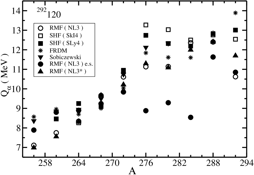
Figure 7: The $Q_{\alpha}$ energy for the $\alpha$-decay chain of the ²⁹²120 nucleus using nonrelativistic SHF (SkI4), SHF (SLy4) and relativistic mean-field formalism (RMF) with NL3* and NL3 parameter set, compared with the FRDM [62] and other theoretical results [29,67,68,69] wherever available.

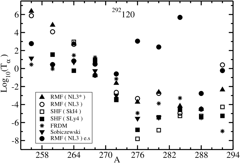
Figure 8: The half-life time $T_{1/2}^{\alpha}$ (in seconds) for the $\alpha$-decay chain of the ²⁹²120 nucleus using nonrelativistic SHF(SkI4), SHF(SLy4) and relativistic mean-field formalism (RMF) with NL3* and NL3 parameter set, compared with the FRDM [62] and other theoretical results [29,67,68,69] wherever available.

We choose the nucleus ²⁹²120 (N = 172) for illustrating our calculations of the $\alpha$-decay chain and the half-life time $T_{1/2}^{\alpha}$. The binding energies of the parent and daughter nuclei are obtained by using both the RMF and SHF formalisms. The $Q_{\alpha}$ values are then calculated; they are shown in Table 3 and 4 and in Figure 7. Then, the half-life $T_{1/2}^{\alpha}$ values are estimated by using the above formulae, and are also given in Table 3 and 4 and in Figure 8. Our predicted results for both $Q_{\alpha}$ and $T_{\alpha}$ for the decay chain of ${}^{292}120$ are compared with the finite range droplet model (FRDM) calculation [67, 68], as well as with the results of other authors [32, 73, 74, 75].

From Figure 7 and 8 and Table 3 and 4, we notice that the calculated values for both $Q_{\alpha}$ and $T_{\alpha}$ agree fairly well with the FRDM predictions, as well as with the other theoretical results available. For example, the value of both $Q_{\alpha}$ and $T_{\alpha}$, in both the FRDM and SHF model, coincides well for the ${}^{288}118$. For ${}^{280}114$ isotope, the SHF (SLy4) prediction also coincides well with the Sobiczewski result for both $Q_{\alpha}$ and $T_{\alpha}$, and the $Q_{\alpha}$ value of RMF with FRDM result. Furthermore, the possible shell structure effects in $Q_{\alpha}$, as well as in $T_{\alpha}$, are noticed for the daughter nucleus ${}^{284}116$ (N = 168) and ${}^{292}120$ (N = 172) in RMF (NL3*) and RMF(NL3), ${}^{262}106$ (N = 156) and ${}^{284}116$ (N = 168) in SHF (SkI4), ${}^{268}108$ (N = 160) and ${}^{284}116$ (N = 168) in SHF (SLy4) and ${}^{284}116$ (N = 168) in FRDM calculations. Note that these proton and neutron numbers refer to either observed or predicted magic numbers.

Table 5: The $Q_{\alpha}$ and $log_{10}T_{1/2}^{\alpha}$ (in sec) for $\alpha$-decay series of ³⁰⁴120 nucleus, calculated in the SHF (SkI4), SHF (SLy4), RMF(NL3*) and RMF(NL3) models, and compared with the Finite Range Droplet Model (FRDM) results [62] and other theoretical results [29,67,68,69] wherever available. In order to compare, we have calculated the $T_{1/2}^{\alpha}$ values in case of Sobiczewski et al. using Eq.(15).

A	Z	Formalism	BE	$\beta_{2}$	$Q_{\alpha}$	$log_{10}T_{1/2}^{\alpha}$
304	120	RMF(NL3*)	2142.57	0.59	10.01	2.14
		RMF(NL3)	2146.37	0.59	9.94	2.37
			2141.34	0.00	12.08	-3.26
		SHF(SKI4)	2134.96	0.00	11.95	-2.95
			2132.61	0.56	11.93	-2.95
		SHF(SLy4)	2112.37	0.01	11.08	-0.83
			2108.29	0.56	11.62	-2.17
		FRDM	2137.99	0.00	13.82	-6.83
		Sobiczewski		0.00	13.07	-5.38
300	118	RMF(NL3*)	2124.29	0.58	9.29	3.78
		RMF(NL3)	2128.01	0.58	9.47	3.18
			2125.12	-0.00	10.74	-0.54
		SHF(SKI4)	2118.60	0.00	11.02	-1.27
			2116.24	0.56	9.82	2.06
		SHF(SLy4)	2095.15	0.01	9.98	1.59
			2091.61	0.54	10.81	-0.73
		FRDM	2123.51	0.00	12.72	-5.18
		Sobiczewski		0.00	11.98	-3.58
296	116	RMF(NL3*)	2105.28	0.54	9.33	2.96
		RMF(NL3)	2109.18	0.54	9.40	2.73
			2107.56	-0.04	9.74	1.66
		SHF(SKI4)	2101.32	0.03	9.88	1.25
			2097.76	0.55	9.36	2.85
		SHF(SLy4)	2076.83	0.04	9.19	3.41
			2074.12	0.53	9.81	1.44
		FRDM	2107.94	-0.01	11.10	-2.08
		Sobiczewski		0.00	10.71	-1.07
292	114	RMF(NL3*)	2086.31	0.51	8.77	4.14
		RMF(NL3)	2090.28	0.51	8.99	3.37
			2089.00	0.06	8.88	3.75
		SHF(SKI4)	2082.90	0.03	7.62	8.59
			2078.82	0.51	9.07	3.12
		SHF(SLy4)	2057.72	0.08	9.49	1.77
			2055.63	0.53	9.25	2.52
		FRDM	2090.75	-0.02	8.25	6.02
		Sobiczewski		0.00	9.60	1.42
288	112	RMF(NL3*)	2066.78	0.49	8.83	3.22
		RMF(NL3)	2070.98	0.49	8.55	4.18
			2069.58	-0.09	9.37	1.46
		SHF(SKI4)	2062.22	0.10	10.04	-0.51
			2059.59	0.52	7.12	9.99
		SHF(SLy4)	2038.91	0.11	8.85	3.65
			2036.58	0.52	8.70	3.13
		FRDM	2070.70	-0.06	8.34	4.92
		Sobiczewski		0.09	9.04	2.51

Table 6: Same as Table 5.

A	Z	Formalism	BE	$\beta_{2}$	$Q_{\alpha}$	$log_{10}T_{1/2}^{\alpha}$
284	110	RMF(NL3*)	2047.31	0.14	7.65	6.87
		RMF(NL3)	2051.23	0.13	7.88	5.92
			2050.65	0.48	7.34	8.11
		SHF(SKI4)	2043.95	0.13	8.02	5.39
			2038.41	0.36	11.98	-5.84
		SHF(SLy4)	2019.46	0.15	8.11	5.05
			2016.98	0.49	8.60	3.27
		FRDM	2050.75	0.10	7.57	7.18
		Sobiczewski		0.10	8.34	4.19
280	108	RMF(NL3*)	2026.66	0.16	7.31	7.49
		RMF(NL3)	2030.81	0.15	7.72	5.77
			2029.69	0.44	6.73	10.14
		SHF(SKI4)	2023.68	0.17	7.71	5.82
			2022.11	0.26	8.58	2.62
		SHF(SLy4)	1999.26	0.17	8.10	4.31
			1997.28	0.43	8.59	2.57
		FRDM	2030.03	0.11	7.56	6.43
276	110	RMF(NL3*)	2005.67	0.17	6.83	8.11
		RMF(NL3)	2010.24	0.17	6.96	8.19
			2008.12	0.41	8.13	3.44
		SHF(SKI4)	2003.08	0.19	7.23	6.97
			2002.35	0.32	7.96	4.06
		SHF(SLy4)	1979.07	0.20	7.64	5.31
			1977.58	0.40	8.74	1.34
		FRDM	2009.28	0.14	7.20	7.13

4.2 The $\alpha$-decay series of ³⁰⁴120 nucleus

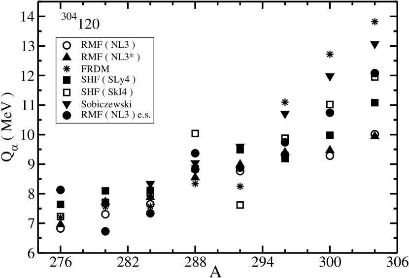
Figure 9: The $Q_{\alpha}$ energy for the $\alpha$-decay chain of the ³⁰⁴120 nucleus using nonrelativistic SHF(SkI4), SHF(SLy4) and relativistic mean-field formalism, (RMF) with NL3* and NL3 parameter set, compared with the FRDM [62] and other theoretical results [29,67,68,69] wherever available.

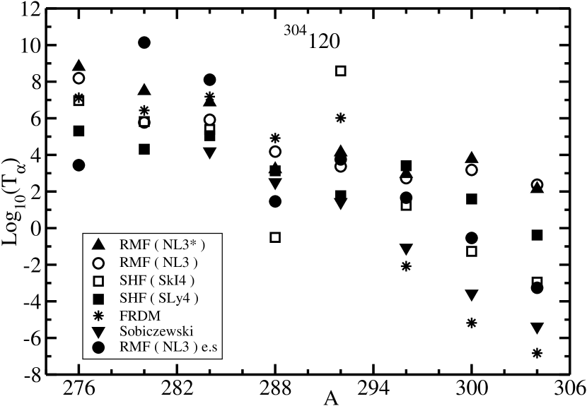
Figure 10: The half-life time $T_{1/2}^{\alpha}$ (in seconds) for the $\alpha$-decay chain of the ³⁰⁴120 nucleus using nonrelativistic SHF(SkI4), SHF(SLy4) and relativistic mean-field formalism (RMF) with NL3* and NL3 parameter set, compared with the FRDM [62] and other theoretical results [29,67,68,69] wherever available.

In this subsection, we present the $Q_{\alpha}$ and $T_{1/2}^{\alpha}$ results for the decay series of ³⁰⁴120 nucleus, using the same procedure as explained in the previous subsection for ²⁹²120 nucleus. The results obtained are listed in Table 5 and 6, and plotted in Figures 9 and 10, compared with the FRDM predictions [67, 68], as well as with the results of other authors [32, 73, 74, 75].

From Figure 9 and Tables 5 and 6, we notice that the calculated values for $Q_{\alpha}$ agree quite well within different models at different mass numbers. For example, the value of $Q_{\alpha}$, in the RMF, SHF and FRDM model, coincides well with the data for ²⁷⁶110 (N = 168) and ²⁸⁰108 (N = 172). Similarly, for ²⁸⁸112 (N = 176) and ²⁹²114 (N = 178), the SHF prediction matches the Sobiczewski et al. result. For ²⁸⁸112 (N = 176) we also have good agreement between RMF and FRDM result. But towards high mass number we do not have agreement within different models. From Figures 10 and Table 5 and 6, we can notice almost similar nature of the half-life time $T_{1/2}^{\alpha}$ values between different models. Possible shell structure effects in $Q_{\alpha}$, as well as in $T_{\alpha}$, are noticed for the daughter nucleus ${}^{284}110$ (N = 174) and ${}^{292}114$ (N = 178) in RMF(NL3*), ${}^{280}108$ (N = 172) in RMF (NL3), ${}^{284}110$ (N = 174) and ${}^{292}114$ (N = 178) in FRDM and in SHF (SkI4), and ${}^{280}108$ (N = 172) and ${}^{284}110$ (N = 174) in SHF (SLy4). Here again we note that these proton and neutron numbers refer to either observed or predicted magic numbers.

5 Summary

Summarizing, we have calculated the binding energy, and quadrupole deformation parameter for the isotopic chain of ²⁹²120 and ³⁰⁴120 superheavy element, which are being planned to synthesize. We employed both the SHF and RMF formalisms using various parameter sets, for both the ground as well as intrinsic first excited states to see the model dependence of the results. We found qualitatively similar predictions in both techniques and the results obtained here also consistents to earlier calculation with different forces [36, 37, 50, 51, 52, 53, 54]. From the calculated binding energy, we also estimated the two-neutron separation energy ($S_{2n}$) and the energy difference ($\triangle E$) between ground state and first excited state for studying the shape coexistence. A shape change from prolate to highly deformed oblate at A = 282, and from highly deformed prolate to highly deformed oblate at A = 320 is observed in RMF formalism. In RMF calculation most of the ground state structures are found to be highly deformed prolate, differing strongly with the FRDM calculation where most of the ground state structures are with spherical solutions. However, in SHF formalism we found that the ground state structures along the whole isotopic chain are prolate. Thus, in RMF formalism most of the isotopes are superdeformed in their ground state configurations, and are low laying highly deformed states in case of SHF formalism. From the binding energy analysis, we found that the most stable isotope in the $Z$=120 series is around ³⁰⁴120, which is near to predicted magic number at N = 184 [118]. Our predicted $\alpha$-decay energy $Q_{\alpha}$ and half-life time $T_{1/2}^{\alpha}$ agree nicely with the FRDM and other available theoretical results [32, 73, 74, 75].

References

- [1] W. D. Myers and W. J. Swiatecki, Report UCRL No. (1965) 11980.
- [2] A. Sobiczewski, F. A. Gareev, and B. N. Kalinkin, Phys. Lett. 22, (1966) 500.
- [3] H. Meldner, in Proceedings of the International Lysekil Symposium, Sweden, August 21-27, 1966.
- [4] H. Meldner, Ark. Fys. 36, (1967) 593.
- [5] U. Mosel and W. Greiner, Z. Phys. 222, (1969) 261.
- [6] H. Ikezoe et al., Eur. Phys. J. A 2, (1998) 379.
- [7] S. Hofmann and G. Münzenberg, Rev. Mod. Phys. 72, (2000) 733.
- [8] Z. G. Gan et al., Eur. Phys. J. A 20, (2004) 385.
- [9] Ch. Stodel et al., AIP Conf. Proc. 891, (2007) 55.
- [10] R.-D. Herzberg, J. Phys. G 30, (2004) 123(R).
- [11] R.-D. Herzberg et al., Nature 442, (2006) 896.
- [12] R.-D. Herzberg and P. T. Greenlees, Prog. Part. Nucl. Phys. 61, (2008) 674.
- [13] S. Hofmann, Prog. Part. Nucl. Phys. 62, (2009) 337.
- [14] K. Morita, Prog. Part. Nucl. Phys. 62, (2009) 325.
- [15] L. Stavsetra et al., Phys. Rev. Lett. 103, (2009) 132502.
- [16] S. Ketelhut et al., Phys. Rev. Lett. 102, (2009) 212501.
- [17] Yu. Ts. Oganessian et al., Phys. Rev. C 83, (2011) 954315.
- [18] S. Hofmann et al., Z. Phys. A 350, (1995) 277.
- [19] S. Hofmann et al., Z. Phys. A 350, (1995) 281.
- [20] S. Hofmann et al., Z. Phys. A 354, (1996) 229.
- [21] S. Hofmann et al., Rep. Prog. Phys. 61, (1998) 639; Acta Phys. Pol. B 30, (1999) 621.
- [22] K. Morita et al., J. Phys. Soc. Jpn. 73, (2004) 2593.
- [23] K. Morita et al., Eur. Phys. J. A 21, (2004) 257.
- [24] K. Morita et al., J. Phys. Soc. Jpn. 76, (2007) 043201.
- [25] T. N. Ginter, Phys. Rev. C 67, (2003) 064609.
- [26] Yu. Ts. Oganessian, Phys. Rev. Lett. 83, (1998) 3154.
- [27] Yu. Ts. Oganessian et al., Nucl. Phys. A 685, (2001) 17c.
- [28] Yu. Ts. Oganessian et al., Phys. Rev. C 69, (2004) 021601(R).
- [29] Yu. Ts. Oganessian, J. Phys. G: Nucl. Part. Phys. 34, (2007) R165.
- [30] Yu. Ts. Oganessian et al., Phys. Rev. Lett. 104, (2010) 142502.
- [31] R. Eichler et al., Nucl. Phys. A 787, (2007) 373c.
- [32] Z. Patyk and A. Sobiczewski, Nucl. Phys. A533, (1991) 132.
- [33] P. Möller and J. R. Nix, Nucl. Phys. A549, (1992) 84.
- [34] P. Möller and J. R. Nix, J. Phys. G20, (1994) 1681.
- [35] S. G. Nilsson, C. F. Tsang, A. Sobiczewski, Z. Szymanski, S. Wycech, C. Gustafson, I.-L. Lamm, P. Möller, and B. Nilsson, Nucl. Phys. A131, (1969) 1.
- [36] K. Rutz, M. Bender, T. Bürvenich, T. Schilling, P. -G. Reinhardt, J. A. Maruhn, and W. Greiner, Phys. Rev. C 56, (1997) 238.
- [37] M. Bender, K. Rutz, P.-G. Reinhard, J. A. Maruhn, and W. Greiner Phys. Rev. C60, (1999) 034304.
- [38] R. K. Gupta, S. K. Patra, and W. Greiner, Mod. Phys. Lett. A 12, (1997) 1727.
- [39] S. K. Patra, C. -L. Wu, C. R. Praharaj, and R. K. Gupta, Nucl. Phys. A 651, (1999) 117.
- [40] Tapas Sil, S. K. Patra, B. K. Sharma, M. Centelles, and X. Viñas, Phys. Rev. C 69, (2004) 044315.
- [41] S. Cwiok, J. Dobaczewski, P. -H. Heenen, P. Magierski , and W. Nazarewicz, Nucl. Phys. A 611, (1996) 211.
- [42] S. Cwiok, W. Nazarewicz, and P. H. Heenen, Phys. Rev. Lett. 83, (1999) 1108.
- [43] A. T. Kruppa, M. Bender, W. Nazarewicz, P.-G. Reinhard, T. Vertse, and S. Cwiok, Phys. Rev. C 61, (2000) 034313.
- [44] A. Marinov, I. Rodushkin, Y. Kashiv, L. Halicz, I. Segal. A. Pape, R. V. Gentry, H. W. Miller, D. Kolb, and R. Brandt, Phys. Rev. C 76, (2007) 021303(R).
- [45] A. Marinov, I. Rodushkin, D. Kolb, A. Pape, Y. Kashiv, R. Brandt, R. V. Gentry, and H. W. Miller, Int. J. Mod. Phys. E 19, (2010) 131.
- [46] A. Marinov, I. Rodushkin, A. Pape, Y. Kashiv, D. Kolb, R. Brandt, R. V. Gentry, H. W. Miller, L. Halicz, and I. Segal, Int. J. Mod. Phys. E 18, (2009) 621.
- [47] S. K. Patra, M. Bhuyan, M. S. Mehta and R. K. Gupta, Phys. Rev. C 80, (2009) 034312.
- [48] G. A. Lalazissis, M. M. Sharma, P. Ring, et al., Nucl. Phys. A 608, (1996) 202.
- [49] W. Long, J. Meng, S. G. Zhou, Phys Rev C, 65 (2002) 047306.
- [50] Z. Ren and H. Toki, Nucl. Phys. A 689, (2001) 691.
- [51] Z. Ren, Phys. Rev. C 65, (2002) 051304(R).
- [52] Z. Ren, D. H. Chen, F. Tai, et al., Phys. Rev. C 67, (2003) 064302.
- [53] Z. Ren, C. Xu, and Z. Wang, Phys. Rev. C 70, (2004) 034304.
- [54] W. Zhang, J. Meng, S. Zhang et al., Nucl. Phys. A 753, (2005) 106.
- [55] H. Zhang, W. Zuo, J. Li et al., Phys. Rev. C 74, (2006) 017304.
- [56] W. Li, N. Wang, J. F. Li et al., Eur. Phys. Lett 64, 750 (2003).
- [57] F. S. Zhang, Z. Q. Feng, G. M. Jin, Int. J. Mod. Phys. E 15, (2006) 1601.
- [58] Z. Q. Feng, G. M. Jin, J. Q. Li et al., Phys. Rev. C 76, (2007) 044606.
- [59] C. Shen, Y. Abe, D. Boilley et al., Int. J. Mod. Phys. E 17, (2008) 66.
- [60] Z. H. Liu and J. D. Bao, Phys. Rev. C 80, (2009) 054608.
- [61] V. Zagrebaev, W. Greiner, Nucl. Phys. A 834, (2010) 366c.
- [62] S. Cwiok, P.-H. Heenen, and W. Nazarewicz, Nature (London) 433, (2005) 705.
- [63] A. Sobiczewski and K. Pomorski, Prog. Part. Nucl. Phys. 58, (2007) 292.
- [64] A. Türler et al., Eur. Phys. J. A 17, (2003) 505.
- [65] G. Audi, O. Bersillon, J. Blachot, and A. H. Wapstra, Nucl. Phys. A 729, (2003) 3.
- [66] A. H. Wapstra, G. Audi, and C. Thibault, Nucl. Phys. A 729, (2003) 129.
- [67] P. Möller, J. R. Nix, W. D. Wyers, and W. J. Swiatecki, At. Data and Nucl. Data Tables 59, (1995) 185.
- [68] P. Möller, J. R. Nix, and K. -L. Kratz, At. Data and Nucl. Data Tables 66, (1997) 131.
- [69] W. D. Myers and W. J. Swiatecki, Nucl. Phys. A 601, (1996) 141.
- [70] S. Liran, A. Marinov, and N. Zeldes, Phys. Rev. C 62, (2000) 047301.
- [71] F. Tondeur, S. Goriely, J. M. Pearson, and M. Onsi, Phys. Rev. C 62, (2000) 024308.
- [72] A. Sobiczewski, Z. Patyk, and S. C. Cwiok, Phys. Lett. 224, (1989) 1.
- [73] I. Muntian, Z. Patyk, and A. Sobiczewski, Acta Phys. Pol. B 32, (2001) 691.
- [74] I. Muntian, S. Hofmann, Z. Patyk, and A. Sobiczewski, Acta Phys. Pol. B 34, (2003) 2073.
- [75] I. Muntian, Z. Patyk, and A. Sobiczewski, Phys. At. Nucl. 66, (2003) 1015.
- [76] I. Muntian and A. Sobiczewski, Phys. Letts. B 586, (2004) 254.
- [77] A. Sobiczewski, Acta Phys. Pol. B 41, (2010) 157.
- [78] E. Chabanat, P. Bonche, P. Hansel, J. Meyer, and R. Schaeffer, Nucl. Phys. A627, (1997) 710.
- [79] E. Chabanat, P. Bonche, P. Hansel, J. Meyer, and R. Schaeffer, Nucl. Phys. A635, (1998) 231.
- [80] J. R. Stone and P.-G. Reinhard, Prog. Part. Nucl. Phys. 58, (2007) 587.
- [81] P.-G. Reinhard and H. Flocard, Nucl. Phys. A 584, (1995) 467.
- [82] B. D. Serot and J. D. Walecka, Adv. Nucl. Phys. 16, (1986) 1.
- [83] W. Pannert, P. Ring, and J. Boguta, Phys. Rev. Lett. 59, (1986) 2420.
- [84] Y. K. Gambhir, P. Ring, and A. Thimet, Ann. Phys. (N.Y.) 198, (1990) 132.
- [85] J. Boguta, A. R. Bodmer, Nucl. Phys. A 292, (1977) 413.
- [86] G. A. Lalazissis, S. Karatzikos, R. Fossion, D. Pena Arteaga, A. V. Afanasjev, and P. Ring, Phys. Lett. B 671, (2009) 36.
- [87] G. A. Lalazissis, J. König, and P. Ring, Phys. Rev. C 55, (1997) 540.
- [88] T. Gonzales-Llarena, J. L. Egido, G. A. Lalazissis, P. Ring, Phys. Lett. B 379, (1996) 13.
- [89] A. V. Afanasjev, J. König, P. Ring, J. L. Egido, L. M. Robledo, Phys. Rev. C 62, (2000) 054306.
- [90] A. V. Afanasjev, T. L. Khoo, S. Frauendorf, G. A. Lalazissis, I. Ahmad, Phys. Rev. C 67, (2003) 024309.
- [91] A. V. Afanasjev, S. Frauendorf, Phys. Rev. C 71, (2005) 064318.
- [92] D. Vretenar, H. Berghammer, P. Ring, Nucl. Phys. A 581, (1995) 679.
- [93] D. Vretenar, G. A. Lalazissis, R. Behnsch, W. Pöschl, P. Ring, Nucl. Phys. A 621, (1997) 853.
- [94] D. Vretenar, N. Paar, P. Ring, G. A. Lalazissis, Phys. Rev. C 63, (2001) 047301.
- [95] D. Vretenar, N. Paar, P. Ring, G. A. Lalazissis, Nucl. Phys. A 692, (2001) 496.
- [96] T. Nikšić, D. Vretenar, P. Finelli, and P. Ring, Phys. Rev. C 66, (2002) 024306.
- [97] G. A. Lalazissis, T. Nikšić, D. Vretenar, and P. Ring, Phys. Rev. C 71, (2005) 024312.
- [98] D. Vretenara, A. V. Afanasjevb, G. A. Lalazissisc, and P. Ring, Phys. Rep. 409, (2005) 101.
- [99] N. Paar , D. Vretenar , E. Khan and G. Coló, Rep. Prog. Phys. 70, (2007) 691.
- [100] T. Nikšić, D. Vretenar, and P. Ring, Phys. Rev. C 78, (2008) 034318.
- [101] T. Gonzales-Llarena, J. L. Egido, G. A. Lalazissis, and P. Ring, Phys. Lett. B 379, (1996) 13.
- [102] P. Ring, Prog. Part. Nucl. Phys. 37, (1996) 193.
- [103] J. Meng, H. Toki, S.-G. Zhou, S.-Q. Zhang, W.-H. Long, L.-S. Geng, Prog. Part. Nucl. Phys. 57, (2006) 470.
- [104] G. A. Lalazissis, D. Vretenar, P. Ring, M. Stoitsov, and L. M. Robledo, Phys. Rev. C 60, (1999) 014310.
- [105] G. A. Lalazissis, D. Vretenar, and P. Ring, Nucl. Phys. A 650, (1999) 133.
- [106] J. Dobaczewski, H. Flocard, J. Treiner, Nucl. Phys. A 422, (1984) 103.
- [107] S. K. Patra, Phys. Rev. C 48, (1993) 1449.
- [108] M. A. Preston and R. K. Bhaduri, Structure of Nucleus (Addison-Wesley), Chap. 8, (1982) 309.
- [109] D. G. Madland and J. R. Nix, Nucl. Phys. A 476, (1981) 1.
- [110] P. Möller and J.R. Nix, At. Data and Nucl. Data Tables 39, (1988) 213.
- [111] S. K. Patra, M. Del Estal, M. Centelles, and X. Viñas, Phys. Rev. C 63, (2001) 024311.
- [112] T. R. Werner, J. A. Sheikh, W. Nazarewicz, M. R. Strayer, A. S. Umar, and M. Mish, Phys. Lett. B 335, (1994) 259.
- [113] T. R. Werner, J. A. Sheikh, M. Mish, W. Nazarewicz, J. Rikovska, K. Heeger, A. S. Umar, and M. R. Strayer, Nucl. Phys. A 597, (1996) 327.
- [114] M. Bhuyan, S. K. Patra, and Raj K. Gupta, Phys. Rev, C 84, (2011) 014317.
- [115] P. Arumugam, B. K. Sharma, S. K. Patra, and R. K. Gupta, Phys. Rev. C 71, (2005) 064308.
- [116] S. K. Patra, R. K. Gupta, B. K. Sharma, P. D. Stevenson, and W. Greiner, J. Phys. G: Nucl. Part. Phys. 34, (2007) 2073.
- [117] S. K. Patra, F. H. Bhat, R. N. Panda, P. Arumugam, and R. K. Gupta, Phys. Rev. C 79, (2009) 044303.
- [118] M. Bhuyan, S. K. Patra, Mod. Phys. Lett. A in press, (2012).
- [119] S. Yoshida, S. K. Patra, N. Takigawa, and C. R. Praharaj, Phys. Rev. C 50, 1398 (1994).
- [120] S. K. Patra, S. Yoshida, N. Takigawa, and C. R. Praharaj, Phys. Rev. C 50, (1994) 1924.
- [121] S. K. Patra and C. R. Praharaj, Phys. Rev. C 47, (1993) 2978.
- [122] J. P. Maharana, Y. K. Gambhir, J. A. Sheikh, and P. Ring, Phys. Rev. C 46, (1992) R1163.
- [123] P. -G. Reinhard and H. Flocard, Nucl. Phys. A584, (1995) 467.
- [124] B. A. Brown, Phys. Rev. C 58, (1998) 220.
- [125] S. K. Patra and C. R. Praharaj, J. Phys. G 23, (1997) 939.
- [126] V. E. Viola, Jr. and G. T. Seaborg, J. Inorg. Nucl. Chem. 28, (1966) 741.