A non-linear damage accumulation fatigue model for predicting strain life at variable amplitude loadings based on constant amplitude fatigue data

Abstract

A new phenomenological technique for using constant amplitude loading data to predict fatigue life from a variable amplitude strain history is presented. A critical feature of this reversal-by-reversal model is that the damage accumulation is inherently non-linear. The damage for a reversal in the variable amplitude loading history is predicted by approximating that the accumulated damage comes from a constant amplitude loading that has the strain range of the particular variable amplitude reversal. A key feature of this approach is that overloads at the beginning of the strain history have a more substantial impact on the total lifetime than overloads applied toward the end of the cycle life. This technique effectively incorporates the strain history in the damage prediction and has the advantage over other methods in that there are no fitting parameters that require substantial experimental data. The model presented here is validated using experimental variable amplitude fatigue data for three different metals.

1 Introduction

One of the most prevalent methods for testing the fatigue properties of a material is to construct a constant amplitude strain-life curve. In this method, a sample is strained cyclically between two strain levels until failure. This test is performed on a number of identical samples at different strain magnitudes, and the results are plotted as a strain-life curve. This “$\frac{\Delta\varepsilon}{2}-2N_{f}$” curve can be fitted to the Basquin-Manson-Coffin, [1, 2, 3] (BMC) equation,

$$\frac{\Delta\varepsilon}{2}=\frac{\Delta\varepsilon_{e}}{2}+\frac{\Delta\varepsilon_{p}}{2}=\frac{\sigma_{f}^{{}^{\prime}}}{E}\left(2N_{f}\right)^{b}+\varepsilon_{f}^{{}^{\prime}}\left(2N_{f}\right)^{c},$$ (1)

where $\frac{\Delta\varepsilon}{2}$ is half of the strain range, $\Delta\varepsilon_{e}$ is the elastic strain, $\Delta\varepsilon_{p}$ is the plastic strain, $\sigma_{f}^{{}^{\prime}}$ is the fatigue strength coefficient, $E$ is the elastic modulus, $b$ is the fatigue strength exponent, $\varepsilon_{f}^{{}^{\prime}}$ is the fatigue ductility coefficient, $c$ is the fatigue ductility exponent, and $2N_{f}$ is the number of reversals until failure. The low cycle fatigue regime is considered a product of plastic deformation, and the high cycle portion is related primarily to elastic deformation. This approach gives a reasonably accurate prediction of sample life at constant amplitude cyclic strains.

However, parts in service are rarely subjected to idealized constant amplitude cyclic strains and instead undergo variable amplitude loading. The Palmgren-Miner (PM) rule is a widely used approach for predicting part lifetime under variable amplitude loading. This method hypothesizes that the damage caused by each stress state in a variable amplitude load history is a function of the number of times that the particular cyclic stress state occurs and the number of cycles it would take for the sample to fail from a constant amplitude history at that stress state. [4] Mathematically the Palmgren-Miner rule is written,

$$\sum_{i=1}\frac{n_{i}}{N_{fi}}=C,$$ (2)

where the sum is taken over all stress states with $i$ denoting a particular state, $n_{i}$ is the number of cycles at the $i$th stress state, $N_{fi}$ is the number of cycles to failure if the sample is cycled under constant amplitude loading at the $i$th stress state, and $C$ is a constant. Based on the assumptions made by the model, $C$ should be $1$; experimentally it is found to range between $0.7$ and $2.2$. This variability is evidence of the failure of the Palmgren-Miner rule to accurately predict fatigue lifetimes. Although it is well known that the Palmgren-Miner rule is inaccurate, its conceptual simplicity and the minimal amount of data necessary for implementation makes it a popular method for estimating fatigue life.

Improving upon the Palmgren-Miner rule has been a major focus of researchers studying variable amplitude fatigue. A good review of cumulative damage and life prediction theories through the end of the last century is presented by Fatemi and Yang. [5]. In recent years models have been developed based on a variety of techniques that couple theories of fracture mechanics and empirical observations. [6, 7, 8, 9, 10, 11, 12, 13, 14, 15] Other methods take into account the residual stresses caused by the plasticity of the material at the crack tip, and crack tip closing phenomena. [16, 17, 18] Although these modeling methods are more accurate than the Palmgren-Miner rule, they require substantially more experimental data to fit the necessary parameters.

In this paper a new method, free of fitting parameters, is demonstrated for estimating strain life under variable amplitude loading. It is unique from other models in that the only data used for input is the constant amplitude strain-life curve and the cyclic stress-strain response. Using this model it is possible to accurately predict the variable amplitude strain life of specimens using a relatively small amount of experimental data that can easily be generated. In the section following this introduction the analytical details of the model are presented. Next the experimental procedure and model implementation are explained. In the results and discussion section the measured and predicted strain lifetimes are presented and compared. The theoretical lifetimes predicted from this model are compared to lifetime predictions presented in the literature. In the final section the paper is succinctly summarized.

2 Model Details

In this model the total damage, $D_{T}$, is the sum of the damage of all reversals, $D_{i}$, ranging from $i=1$ to $i=2N_{T}$,

$$D_{T}=\sum_{i=1}^{2N_{T}}D_{i}.$$ (3)

In this definition $D_{i}$ is the normalized damage caused by the $i$th reversal and failure occurs when $D_{T}=1$. The damage caused by each reversal is determined using the well-known constant amplitude strain-life relation. Using this approach, the strain history is incorporated as damage accumulation. The damage accrued in each step is calculated using a relatively simple algorithm and constant amplitude strain-life data.

Following examples from Ref. [5], the damage during fatigue is assumed to be due to a single critical crack propagating across the width of the specimen. A good description of the crack growth per reversal, for a constant amplitude strain, is given by the hyperbolic sine function. For a crack size, $a$, the rate of crack tip advance, after $2N_{k}$ reversals, can be written

$$\frac{da}{dN}\propto\sinh\left(\frac{2N_{k}}{2N_{f}}\rho\right),$$ (4)

where $2N_{f}$ is the total number of reversals to failure for the given strain amplitude, and $\rho$ is a scaling factor, which will be discussed in more detail later. Eq. (4) is a natural expression of damage per reversal, and has the same functional form as has been used to describe changes in crack growth rates previously. [19, 5] It accurately reflects the phenomena in that during the initial stages of damage the rate of crack propagation is low and as damage is accrued the rate of crack growth increases. Other expressions for the rate of crack tip advance, which are phenomenologically similar, are presented elsewhere and will not be discussed here. [19, 5]

Using Eq. (4) for damage, the normalized damage due to the $i$th reversal is expressed,

$$D_{i} =\frac{\sum_{k=1}^{N_{T}+1}\sinh\left(\frac{2N_{k}}{2N_{f}}\rho\right)-\sum_{k=1}^{N_{T}}\sinh\left(\frac{2N_{k}}{2N_{f}}\rho\right)}{\sum_{j=1}^{N_{f}}\sinh\left(\frac{2N_{j}}{2N_{f}}\rho\right)}$$ (5)

$$\approx\frac{\int_{N_{T}}^{N_{T}+1}\sinh\left(\frac{2N_{k}}{2N_{f}}\rho\right)dN_{k}}{\int_{1}^{N_{f}}\sinh\left(\frac{2N_{j}}{2N_{f}}\rho\right)dN_{j}},$$

where $N_{T}$ is the number of reversals required to achieve the accumulated damage, $D_{T}$, were the damage due to a constant amplitude strain range, $\frac{\Delta\varepsilon_{i}}{2}$. The number of reversals to failure at this constant strain range is $2N_{f}$. The denominator normalizes the damage per reversal such that at failure the total damage is 1.

The current state of damage, $D_{T}$, is known and is expressed as the sum of incremental damage, $D_{i}$, from Eq. (5),

$$D_{T} =\frac{\sum_{k=1}^{N_{T}}\sinh\left(\frac{2N_{k}}{2N_{f}}\rho\right)}{\sum_{j=1}^{N_{f}}\sinh\left(\frac{2N_{j}}{2N_{f}}\rho\right)}$$ (6)

$$\approx\frac{\int_{1}^{N_{T}}\sinh\left(\frac{2N_{k}}{2N_{f}}\rho\right)dN_{k}}{\int_{1}^{N_{f}}\sinh\left(\frac{2N_{j}}{2N_{f}}\rho\right)dN_{j}},$$

where $N_{T}$ is the number of damaging reversals to cause the damage $D_{T}$ at the constant amplitude strain $\frac{\Delta\varepsilon}{2}$. The summations in Eqs. (5) and (6) can be approximated as integrals, which allows Eq. (6) to be solved to find

$$2N_{T}=\left(\frac{2N_{f}}{\rho}\right)\times$$ (7)

$$\cosh^{-1}\left(D_{T}\left(\cosh\left(\rho\right)-\cosh\left(\frac{\rho}{2N_{f}}\right)\right)+\right.$$

$$\left.\cosh\left(\frac{\rho}{2N_{f}}\right)\right).$$

The general approach for calculating a specimen life under variable amplitude loading goes as follows. Begin by determining the initial total damage. This is typically near zero, if the part begins pristine and the strain-life curve is well defined at all strains of interest. A case for non-zero starting damage will be discussed later in section 4. The strain range for the first tensile reversal is $\frac{\Delta\varepsilon_{1}}{2}$, and $D_{1}$ is calculated using Eq. (5) and the BMC relation, Eq. (1), which is fit to constant amplitude strain life data. The value of $D_{1}$ is added to $D_{T}$. The next tensile strain is $\frac{\Delta\varepsilon_{2}}{2}$. The lifetime at this strain range along with $D_{T}$, are used to calculate $N_{T}$ from Eq. (7), which is used in Eq. (5) to calculate $D_{2}$, which is again added to $D_{T}$. This process continues until $D_{T}=1$, at which point failure is predicted. An algorithm for implementing this model is demonstrated in section 4.

3 Experimental Data

Published experimental data are used to validate the model. [20, 21] Pereira et al. tested P355NL1 steel and compared their experimental results to an effective strain damage model based on the work of DuQuesnay. [20] Colin and Fatemi published experimental data for 304L stainless steel and 7075 T6 aluminum. [21]

The load histories used in the calculations were recreated from the descriptions detailed by Pereira et al., and Colin and Fatemi. [20, 21] The P355NL1 specimens were subjected to a variety of load blocks, including a high to low scheme, a low to high scheme, a low to high to low scheme, and random loading, examples of which are shown in Figs. 1, 2, 3, and 4. The 304L stainless steel fatigue-life results were prepared for periodic, fully-reversed overloads, shown in Fig. 5, and random loading. The 7075 T6 aluminum samples were subjected to random loading. Unlike the shaped loading blocks, the random load history was not reproduced from the literature, but instead a strain history file was created using a random number generator, filtering the random number stream to ensure that each iteration reversed the strain. A representative sample of the random reversal data is shown in Fig. 4.

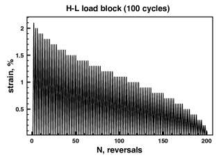
Figure 1: An example of a high to low strain loading block after the work of Pereira et al. [20]

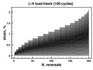
Figure 2: An example of a low to high strain loading block after the work of Pereira et al. [20]

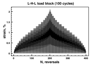
Figure 3: An example of a low to high to low strain loading block after the work of Pereira et al. [20]

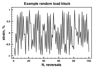
Figure 4: An example of random loading. Note that the random number stream was filtered to ensure that each iteration reversed the direction of the applied strain.

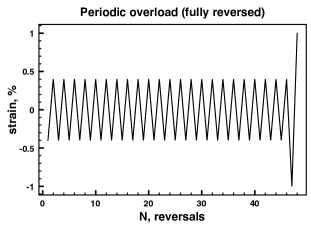
Figure 5: An example of a fully reversed periodic overload loading block after the work of Colin and Fatemi. [21]

4 Model Implementation

The model described in section 2 above was implemented using the algorithm detailed in this section and applied to the strain history data discussed in section 3. To begin, the first two strains from the strain history were converted to stresses using the Ramberg-Osgood stress-strain relationship,

$$\varepsilon=\frac{\sigma}{E}+\left(\frac{\sigma}{K^{{}^{\prime}}}\right)^{1/n^{\prime}},$$ (8)

where $K^{{}^{\prime}}$ and $n^{\prime}$ were fit from the cyclic stress-strain behavior. The Morrow mean stress correction [22],

$$\frac{\Delta\varepsilon}{2}=\frac{\sigma^{{}^{\prime}}_{f}-\sigma_{m}}{E}\left(2N_{f}\right)^{b}+\varepsilon^{{}^{\prime}}_{f}\left(2N_{f}\right)^{c},$$ (9)

where $\sigma_{m}=\frac{\sigma_{i+1}+\sigma_{i}}{2}$ is the mean stress, was used to calculate $N_{f}$. The value of $N_{f}$ was used with $D_{T}$ to calculate $N_{T}$ from Eq. (7). Finally, the damage from this reversal, $D_{i}$, was determined from Eq. (5). The damage was added to the total damage, $D_{T}$. If the total damage was greater than $1$, then the specimen was deemed to have failed due to this reversal, otherwise the procedure was continued using the new value of $D_{T}$ and the next strain taken from the strain history. This was repeated until failure occurs, when $D_{T}\geq 1$.

The constant $\rho$, in Eq. (4), appropriately scales the incremental damage. For this implementation it was selected to be $\rho=\log\left(2N_{f}^{\gamma}\right)$, where $2N_{f}$ was from the BMC equation and $\gamma$ was taken as $-c/2\varepsilon_{f}^{{}^{\prime}}$. In this way, $\rho$ scales with the applied strains and the incremental damage, $da/dN$, has the correct functional relationship to the strain amplitude.

The integrated $da/dN$ curve, which expresses total damage as a function of the number of cycles, has a general shape that is well known. [5, 19, 6, 7] Careful inspection of experimental data of damage as a function of number of cycles reveals that a smooth well fitting curve does not always intercept the damage axis at $0$. In many experiments, damage has been observed to accumulate rapidly to around 5 to 10% early in the specimen’s life, and then slow to the $da/dN$ crack propagation model that is well known. [19, 6, 7] To account for the rapid damage accumulation that occurs during the initial cycling, the starting damage was assigned to be $D_{T}=0.05$ for all of the variable amplitude lifetime prediction data presented here.

5 Results and Discussion

A comparison of the published experimental data and the predictions of this work can be seen in Figs. 6–10. In Figs. 6 and 7 the experimental data for P355NL1 steel, from Pereira et al., is shown for a maximum strain of 1.05% and 2.10% for the loading blocks discussed in section 3 above. [20] The experimental results are compared to those predicted from the present model in addition to the model of Pereira and DuQuesnay. The current model is in good agreement with both the experimental and theoretical results from Peirera et al.

The experimental results from Colin and Fatemi for 304L stainless steel are shown in Figs. 8 and 9 for the loading blocks discussed above at various strain ranges. [21] The results for 7075 T6 aluminum are shown in Fig. 10. The accuracy of the present model is compared to the predictions of the Palmgren-Miner rule both with and without the Smith-Watson-Topper correction. The current model is again in good agreement with the experimental results. It is worth noting that the model presented here agrees with the experimental data both when the Palmgren-Miner results are non-conservative by an order of 2 or 3 and when they agree well with experiment. This is evidence that the results form the current work are more profound than a simple lifetime reduction from the Palmgren-Miner rule.

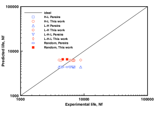
Figure 6: A comparison of this work and the work of Pereira et al. for P355NL1 steel specimens tested by Pereira et al. and presented in Ref. [20]. A variety of load schemes are used at a maximum strain of 1.05%.

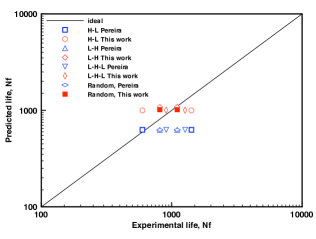
Figure 7: A comparison of this work and the work of Pereira et al. for P355NL1 steel specimens tested by Pereira et al. and presented in Ref. [20]. A variety of load schemes are used at a maximum strain of 2.1%.

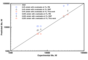
Figure 8: A comparison of the predictions of this work to the Palmgren-Miner rule (PM) with and without a Smith-Watson-Topper correction (SWT) prepared by Colin and Fatemi for 304L stainless steel specimens. [21] The data here represent specimens subjected to a constant amplitude fully reversed strain history punctuated by periodic fully reversed overloads.

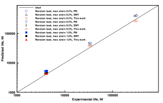
Figure 9: A comparison of the predictions of this work to the Palmgren-Miner rule (PM) with and without a Smith-Watson-Topper correction (SWT) prepared by Colin and Fatemi for 304L stainless steel specimens. [21]The data here represent specimens subjected to random loading.

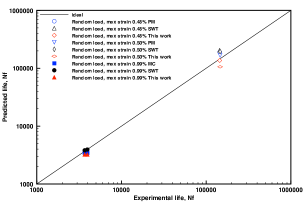
Figure 10: A comparison of the predictions of this work to the Palmgren-Miner rule (PM) with and without a Smith-Watson-Topper correction (SWT) prepared by Colin and Fatemi for 7075-T6 aluminum specimens. [21] The data here represent specimens subjected to random loading.

The strength of the present model is due to the natural inclusion of the strain history when determining the inflicted damage caused by a strain reversal. Both the effect of the immediately preceding strain and the effect of the relative age of a specimen are included. To calculate $\Delta\varepsilon$ a strain and the immediately preceding strain must be known to determine the applied strain range and the mean stress correction. The damage inflicted by a particular strain reversal depends not only on the amplitude, but also on the total state of damage at the instant of the reversal. Take the example of a periodic, fully-reversed, overload. If one considers the integrated $da/dN$ curve for a constant amplitude cyclic strain, applying a fully reversed overload would advance the position of the subsequent constant amplitude reversals on this curve substantially. From the shape of the curve, it is apparent that an overload early in the specimen’s life that increments the damage will have a more substantial impact on the specimen’s total life, compared to an overload applied later.

The more recent models, such as those of [16, 17, 18], include residual strains and crack-tip plasticity or crack tip closure phenomena. These models account for the cumulative damage through localized plasticity near the crack tip, or a change in the effective stresses due to crack tip closure. They are more accurate than the Palmgren-Miner model and other simple models because they account for the ordering of the applied strains and localized damage near the crack tip; however, they require substantial experimental support. By comparison, the present model only includes materials information from the cyclic stress-strain curve and the constant amplitude strain life curve. It should be noted that for some analysis involving extreme load cases, a more sophisticated model than the one presented here may be necessary. In particular, cases where residual plasticity will play a dominant role in crack growth rates through strain hardening and residual stresses will likely require a model that explicitly deals with plasticity near the crack tip.

6 Summary

One of the greatest engineering challenges of the last $100$ years is that of predicting the strain-life relationships of mechanical components undergoing variable amplitude loading. In spite of extensive studies, no conclusive model has been determined. Although many useful models have been developed, many require cumbersome amounts of experimental data. Here we report a new method, free of fitting parameters, for making an accurate variable amplitude strain-life prediction using basic constant amplitude fatigue data. The method is validated using data from experiments performed on P355NL1 steel, 304L stainless steel, and 7075 T6 aluminum. [20, 21] The present model fits the experimental data well for a variety of load spectra and materials and the algorithm is simple to implement.

7 Acknowledgements

The authors gratefully acknowledge funding from John Deere & Company.

References

- Basquin [1910] O. H. Basquin, The Experimental Law of Endurance Tests, In: Proc. ASTM Vol. 10, p. 625, American Society for Testing and Materials, ASTM International, West Conshohocken, PA, 2011, www.astm.org, 1910.
- Manson [1953] S. S. Manson, Behavior of Materials Under Conditions of Thermal Stress, NACA TN 2933, National Advisory Committee for Aeronautics, 1953.
- Coffin [1954] L. F. Coffin, A study of the Effects of Cyclic Thermal Stresses on a Ductile Metal, Trans. ASME, Vol 76 (no.6) p. 931-950, 1954.
- Miner [1945] M. Miner, Cumulative damage in fatigue, J. Appl. Mech.-Trans. ASME 12 (1945).
- Fatemi and Yang. [1998] A. Fatemi, L. Yang., Cumulative fatigue damage and life prediction theories: A survey of the state of the art for homogeneous materials, Int. J. Fatigue 20 (1998) 9–34.
- Sun et al. [2007] B. Sun, L. Yang, Y. Guo, A high cycle fatigue accumulation model based on electrical resistance for structural steels, Fatigue Fract. Eng. Mater. Struct.. 30 (2007) 1052–1062.
- Shang and Yao [1999] D. Shang, W. Yao, A nonlinear damage cumulative model for uniaxial fatigue, Int. J. Fatigue 21 (1999) 187–194.
- Ghammouri et al. [2010] M. Ghammouri, M. Abbadi, J. Mendez, S. Belouettar, M. Zenasni, An approach in plastic strain-controlled cumulative fatigue damage, Int. J. Fatigue 33 (2010) 32–42.
- Risitano and Risitano [2010] A. Risitano, G. Risitano, Cumulative damage evaluation of steel using infrared thermography, Theor. Appl. Fract. Mech. 54 (2010) 82–90.
- Huang et al. [2010] Z. Y. Huang, D. Wagner, J. L. Bathias, C.and Chaboche, Cumulative fatigue damage in low cycle fatigue and gigacycle fatigue for low carbon-manganese steel, Int. J. Fatigue 33 (2010) 115–121.
- Besel et al. [2010] M. Besel, A. Brueckner-Foit, F. Zeismann, A. Gruening, J. Mannel, Damage accumulation of graded steel, Eng. Fail. Anal.. 17 (2010) 633–640.
- Shi et al. [2011] Y. J. Shi, M. Wang, Y. Q. Wang, Experimental and constitutive model study of structural steel under cyclic loading, J. Constr. Steel. Res. 67 (2011) 1185–1197.
- Aid et al. [2011] A. Aid, A. Amrouche, B. B. Bouiadjra, M. Benguediab, G. Mesmacque, Fatigue life prediction under variable loading based on a new damage model, Mater. Des. 32 (2011) 183–191.
- Rejovitzky and Altus [2011] E. Rejovitzky, E. Altus, Non-commutative fatigue damage evolution by material heterogeneity, Int. J. Fatigue. 37 (2011) 54–59.
- Chen et al. [2011] H. Chen, D. Shang, E. Liu, Multiaxial fatigue life prediction method based on path-dependent cycle counting under tension/torsion random loading, Fatigue Fract. Eng. Mater. Struct. 34 (2011) 782–791.
- Noroozi and Lambert [2008] G. Noroozi, A.H.and, S. Lambert, Prediction of fatigue crack growth under constant amplitude loading and a single overload based on elasto-plastic crack tip stresses and strains, Eng. Fract. Mech. 75 (2008).
- Halliday and Bowen [2011] M. Halliday, P. Bowen, Fatigue extrusions, slip band cracking and a novel hybrid concept for fatigue crack closure close to the crack tip, Int. J. Fatigue 33 (2011).
- Shanyavskiy [2011] A. Shanyavskiy, Fatigue cracking simulation based on crack closure effects in al-based sheet materials subjected to biaxial cyclic loads, Eng. Fract. Mech. 78 (2011).
- Lemaitre and Chaboche [1985] J. Lemaitre, J.-L. Chaboche, Mechanics of Solid Materials, Press Syndicate of the University of Cambridge, New York, New York, 1985.
- Pereira et al. [2009] H. Pereira, D. L. DuQuesnay, A. M. P. De Jesus, A. L. L. Silva, Analysis of variable amplitude fatigue data of the p355nl1 steel using the effective strain damage model, J. Press. Vessel Technol.-Trans. ASME 131 (2009).
- Colin and Fatemi [2010] J. Colin, A. Fatemi, Variable amplitude cyclic deformation and fatigue behaviour of stainless steel 304l including step, periodic, and random loadings, Fatigue Fract. Eng. Mater. Struct.. 33 (2010) 205–220.
- Socie and Morrow [1980] D. Socie, J. Morrow, Risk and Failure Analysis for Improved Performance and Reliability (Edited by J. J. Burke & V. Weiss), Plenum Publication Corp., New York, NY, 1980.