A high molecular fraction in a sub-damped absorber at $\mn@boldsymbol{z=0.56}$

Abstract

Measuring rest-frame ultraviolet rotational transitions from the Lyman and Werner bands in absorption against a bright background continuum is one of the few ways to directly measure molecular hydrogen (H₂). Here we report the detection of absorption from H₂ at $z=0.56$ in a sub-damped Ly$\alpha$ system with neutral hydrogen column density $N_{\textsc{H\,i}}$ $=10^{19.5\pm 0.2}$ cm^-2. This is the first H₂ system analysed at a redshift $<1.5$ beyond the Milky Way halo. It has a surprisingly high molecular fraction: log₁₀ $f_{\textrm{H}_{2}}$ $>-1.93\pm 0.36$ based on modelling the line profiles, with a robust model-independent lower limit of $f_{\textrm{H}_{2}}$ $>10^{-3}$. This is higher than $f_{\textrm{H}_{2}}$ values seen along sightlines with similar $N_{\textsc{H\,i}}$ through the Milky Way disk and the Magellanic clouds. The metallicity of the absorber is $0.19^{+0.21}_{-0.10}$ solar, with a dust-to-gas ratio $<0.36$ of the value in the solar neighbourhood. Absorption from associated low-ionisation metal transitions such as O i and Fe ii is observed in addition to O vi. Using Cloudy models we show that there are three phases present; a $\sim 100$ K phase giving rise to H₂, a $\sim 10^{4}$ K phase where most of the low-ionisation metal absorption is produced; and a hotter phase associated with O vi. Based on similarities to high velocity clouds in the Milky Way halo showing H₂, and the presence of two nearby galaxy candidates with impact parameters of $\sim 10$ kpc, we suggest that the absorber may be produced by a tidally-stripped structure similar to the Magellanic Stream.

1 Introduction

Molecular hydrogen (H₂) is the most abundant molecule in the universe and is closely linked to star formation via the star formation surface density rate – molecular gas surface density relation (Bigiel et al., 2008). Measuring rest-frame UV rotational transitions from the Lyman and Werner bands in absorption against a bright background continuum is one of the few ways to directly measure H₂ (see Draine, 2011, for example). This technique probes diffuse gas with molecular fractions, $f_{\textrm{H}_{2}}$, of $\sim 10^{-6}$ to $\sim 0.1$ – denser molecular clouds are both dusty, and thus likely to extinguish UV light from a background source, and compact, such that there is a low probability of intersection with a sightline to a background light source (Hirashita et al., 2003; Zwaan & Prochaska, 2006). However, the lower molecular fraction systems that are detected give valuable insights into the environments and physical mechanisms necessary for the formation of H₂. With this technique we can measure the physical properties of cool, dense gas over a large fraction of the age of the Universe, from the interstellar medium in the solar neighbourhood to proto-galaxies a few Gyr after the big bang.

Since the initial detection towards the UV bright star $\xi$ Persei (Carruthers, 1970), a large sample of sightlines exhibiting H₂ in absorption from the Milky Way and its halo has been assembled. These observations have characterised H₂ in diffuse molecular gas in the Milky Way plane (Savage et al., 1977), the Magellanic clouds (Tumlinson et al., 2002; Welty et al., 2012), high latitude sightlines out of the Milky Way plane (Gillmon et al., 2006; Wakker, 2006), in intermediate and high velocity clouds (IVCs and HVCs, Richter et al., 2003, 1999), and in the Magellanic Stream (Sembach et al., 2001; Richter et al., 2001). A physical picture where H₂ formation occurs predominantly on the surface of dust grains (Shull & Beckwith, 1982) in clouds with total densities of $n\sim 10-100$ cm^-3 illuminated by the local UV radiation has been successful in reproducing both the observed H₂ rotational population levels and molecular fractions in the Milky Way (for example Spitzer et al. 1974; Jura 1975a,b) and the Magellanic clouds (Tumlinson et al., 2002).

H₂ has also been measured at redshifts $1.5-4.5$, corresponding to lookback times of $\sim 9-12$ Gyr, in damped Ly$\alpha$ ($N_{\textsc{H\,i}}$ $>10^{20.3}$ cm^-2, DLA) and sub-damped Ly$\alpha$ ($10^{19}$ cm^-2 $\lesssim$ $N_{\textsc{H\,i}}$ $\lesssim 10^{20.3}$ cm^-2, sub-DLA) absorption systems seen towards bright background QSOs. In this redshift range, absorption features from H i and sometimes H₂ are redshifted into the optical range, making them relatively easy to detect with large ground-based telescopes. The first unambiguous detection in a redshifted absorber was made by Foltz et al. (1988, see also Levshakov & Varshalovich, 1985), and since then at least $16$ further such systems have been discovered (for example Ge & Bechtold, 1997; Ge et al., 2001; Levshakov et al., 2002; Cui et al., 2005; Ledoux et al., 2006; Noterdaeme et al., 2007). Approximately $10$ per cent of DLAs have a molecular fraction $f_{\textrm{H}_{2}}$ $>10^{-4.5}$, and these tend to be more metal rich and dustier (Ledoux et al., 2003), and have higher velocity widths (Noterdaeme et al., 2008) than DLAs without detectable H₂. Several physical diagnostics are available to measure the properties of the H₂ absorbing gas. Some H₂ systems also show absorption from the CO molecule, revealing the presence of a cold, dense core of gas with excitation temperatures consistent with those expected from the cosmic microwave background (for example Srianand et al., 2008; Noterdaeme et al., 2009). The H₂ rotational level populations and C i fine structure transitions can also be used to measure particle densities. They are generally found to be similar to those measured along local sightlines in the Milky Way ($\sim 10-100$ cm^-3), but the ambient UV field, gas temperatures and gas pressures tend to be higher (Hirashita & Ferrara, 2005; Srianand et al., 2005).

No studies currently exist of H₂ at lower redshifts, $z<1.5$, outside the Milky Way halo. Until recently, the low number of DLA and sub-DLA systems known at low redshifts, together with the smaller light gathering power of spaced-based UV telescopes compared to large aperture ground-based optical telescopes, have made observing the Lyman-Werner bands in this redshift range impractical. However, with the availability of the far-UV sensitive Cosmic Origins Spectrograph (COS) on the Hubble Space Telescope (HST), molecular absorption can now be effectively detected for $0.1\lesssim z\lesssim 0.8$.

In this paper we report the serendipitous detection of H₂ in a sub-DLA at $z=0.56$, the first such system analysed at a redshift below $1.5$ beyond the Milky Way halo. It has a high molecular fraction given the total cloud neutral hydrogen column density, and we show that the associated metal absorption features seen require the presence of three phases: a cold $T\sim 100$ K phase analogous to the cold neutral medium observed in the Milky Way’s interstellar medium (ISM); a partially-ionised $T\sim 10^{4}$ K phase, similar to the warm neutral medium in the ISM; and a warmer, probably collisionally ionised phase. Based on the cloud properties we argue the absorber is likely caused by a tidally-stripped absorbing structure similar to the Magellanic Stream embedded in a warm halo $\sim 10$ kpc from a nearby galaxy.

The layout of the paper is as follows. Section 2 describes the data used; Section 3 describes how we identified lines and measured the absorption line properties; and Section 4 describes the properties of the H₂ absorption and the sub-DLA. We compare to theoretical models and discuss our results in Section 5, and summarise the main results of the paper in Section 6. When not explicitly shown logarithms are to base 10, and we use a 7-year WMAP cosmology ($H_{0}=70.4$ km s^-1 Mpc^-1, $\Omega_{\mathrm{M}}=0.272$, $\Omega_{\Lambda}=0.728$; Komatsu et al., 2011) where necessary. We use transition wavelengths and oscillator strengths given by Morton & Dinerstein (1976); Morton (2003) and Verner et al. (1994), and H₂ transition wavelengths from Bailly et al. (2010).

2 Data

Transitions from the sub-DLA are measured in absorption against the continuum from the background QSO, Q 0107$-$0232, at $z_{\rm qso}=0.728$ (see Table 1). This was discovered by the Large Bright Quasar survey (Hewett et al., 1995) and is one of a group of three bright QSOs with small angular separations on the sky. Spectra of these QSOs taken using the Faint Object Spectrograph (FOS) on the HST have been used to measure correlations in neutral hydrogen absorption (Young et al., 2001; Petry et al., 2006) and in absorption with galaxy positions (Crighton et al., 2010) across the three sightlines.

Here we present higher resolution far UV spectra of Q 0107$-$0232 taken with the Cosmic Origins Spectrograph on the HST, and an optical spectrum taken with the High Resolution Echelle Spectrograph (HIRES) on Keck I. In our analysis we also make use of $K$ band imaging of the QSO and archival UV FOS spectra. The FOS spectra were originally published by Young et al. (2001). We employ the combined spectrum used by Crighton et al. (2010), covering a wavelength range of $1572-2311\,$Å at a typical signal to noise (S/N) of $31$ per $4\,$Å resolution full width at half maximum intensity (FWHM).

Name	R.A. (J2000)	Dec. (J2000)	$z_{\rm em}$	$R$-mag
Q 0107$-$0232	$01^{\mathrm{h}}10^{\mathrm{m}}14.43^{\mathrm{s}}$	$-02\degr 16\arcmin 57.6\arcsec$	$0.728$	$18.4$

Table 1: Properties of the background QSO towards which the sub-DLA is seen. Columns show the coordinates, emission redshift (measured from Mg ii $\lambda\lambda\ 2296,2803$ emission in the HIRES spectrum) and $R$ band magnitude.

Dataset	Date obs.	Exp. Time (s)	Grating	$\lambda_{\rm c}$ (Å)
LB5H12010	6 Nov 2010	$13905.728$	G160M	$1589$
LB5H13010	18 Nov 2010	$13905.472$	G160M	$1589$
LB5H11010	19 Nov 2010	$13905.376$	G160M	$1589$
LB5H14010	24 Nov 2010	$13905.536$	G160M	$1623$
LB5H15010	26 Nov 2010	$13905.504$	G160M	$1623$
LB5H16010	7 Dec 2010	$13905.472$	G160M	$1623$

Table 2: Observations of Q 0107$-$0232 with HST/COS. Columns show the HST archive dataset name, the date observed, total exposure time, grating and central wavelength setting used.

2.1 COS spectra reduction

The COS spectra were obtained over a period from the 6th of November to the 7th of December 2010, as part of the Cycle 17 proposal 11585. They represent a total exposure time of $23$ hours across $30$ orbits. Two central wavelength settings were taken with the G160M grating, each using $4$ FP-POS positions to enable complete wavelength coverage from $1380$ to $1850$ Å. Details of the exposures are given in Table 2.

We used the CALCOS pipeline to perform background subtraction, wavelength calibration and extraction. The default background extraction smoothing scale of $100$ pixels resulted in poor background subtraction for our spectra, presumably because the pipeline was optimised for brighter targets. We found that changing BWIDTH in the XTRACTAB calibration table from the default value of 100 to $20$ significantly improved the background level such that the flux in strongly saturated features broader than the COS instrument line spread profile was consistent with zero.

Wavelength shifts are expected between visits and different wavelength settings due to temperature differences and uncertainty in the telescope pointing. The S/N in individual exposures is generally too low ($\sim 2$ per pixel) to reliably measure the centres of absorption features. Therefore we combined subsets of exposures grouping by FP-POS position, by visit (corresponding to a single dataset name in Table 2), by grating central wavelength and by FUV segment to search for any shifts. Wavelength solutions were consistent across different visits and FP-POS values, but there are significant wavelength-dependent shifts between different central wavelength settings. To correct these, we measured the centroid for common narrow absorption features where two wavelength settings overlapped, and used these centres to calculate a wavelength offset as a function of position. We fitted these offsets with a linear dependence on wavelength, and then corrected for them such that FUV segment A $\lambda_{c}=1627$ matched the FUV segment A $\lambda_{c}=1589$ setting, and FUV segment B $\lambda_{c}=1589$ matched the FUV segment B $\lambda_{c}=1627$ setting. The largest shifts applied in this way were $0.1$ Å, corresponding to $20$ km s^-1, but they could result in a $\sim 40$ km s^-1 internal shift between the shortest and longest wavelengths of an exposure. These shifts are given in Table 6.

The scores of H₂ absorption features distributed across the full spectral range enable a further check of the internal consistency of the wavelength solution. By measuring the centroid of these features and comparing to a single-component model of H₂ absorption, we discovered an additional wavelength-dependent shift (shown in Table 7). The magnitude of this shift is smaller ($\sim 5$ km s^-1) than that applied above, but still significant when fitting an absorption system with transitions spread across a large wavelength range. We removed this shift by subtracting a cubic spline fitted to the offsets as a function of wavelength position from the wavelength scale.

To match the zero points of the COS and HIRES wavelength scales, we compared the N ii $1084$ and C i $945$ features from the $z=0.56$ system in the combined COS spectrum to their expected positions from the redshifts of the Fe ii and Mg ii lines from the same system measured in the HIRES spectrum. The wavelength zero point of the HIRES spectrum is known to better than 1 km s^-1 relative to narrow Galactic Ca ii absorption features seen in the spectrum. Both the N ii and C i appear at redshifts expected from the HIRES Fe ii and Mg ii redshifts, and N ii shows a similar component structure (albeit at the lower COS resolution). We conclude that no correction to the wavelength zero point of the combined COS spectrum is necessary.

We also measured the redshift of Galactic absorption features in the COS spectrum to confirm the zero point of the wavelength solution was correct. These are all saturated and possibly contain multiple components, so do not provide a stringent constraint on the zero point. However, they show no evidence of a systematic offset.

After correcting each exposure for these wavelength shifts we made a combined spectrum in the following way. First we rebinned each exposure to a single wavelength scale with pixel width $0.0367$ Å, ensuring Nyquist sampling. We used nearest-neighbour binning to preserve the spectra’s noise properties, and checked that this did not introduce any significant wavelength shifts. The $1\sigma$ uncertainty on each pixel was estimated empirically as the standard error on the mean of the contributing pixel fluxes. This is a slight overestimate of the true uncertainty, as the exposure times were not all identical. However, the uncertainties measured in this way are consistent with the standard deviation of the flux in regions free from absorption, and we believe this is a good estimate of the true uncertainty.

Since the background level of the COS spectra is low, at small source count rates the flux distribution may be better described by Poisson rather than Gaussian statistics. However, in practice we find that for regions of our spectra with the lowest number of counts – the cores of saturated profiles – uncertainties in the background levels from the many contributing exposures makes a Gaussian flux distribution a good approximation.

Finally we estimated the unabsorbed continuum level of the combined spectrum by fitting spline segments joining regions that appeared free from absorption. The resulting combined spectrum has a S/N of $10$ per $\sim 20$ km s^-1 resolution element at the continuum and covers a wavelength range from $1380$ to $1850$ Å.

2.2 HIRES spectra reduction

The HIRES observations were performed on the night of 4th of August 2011. Four 1800 s exposures were taken using the red cross-disperser and a 0.861″ width slit. Two wavelength settings were used to cover gaps in the detector. We used MAKEE to process each exposure, which subtracts the bias level and the sky background, corrects for the echelle blaze, generates a wavelength solution by identifying arc lines to yield a mapping from pixel number to wavelength for each echelle order, and extracts one-dimensional spectra for each echelle order. We then used custom-written Python code to coadd the individual orders for each exposure into a combined spectrum, and to infer the unabsorbed continuum level by fitting spline segments to regions free from absorption. The final combined spectrum has a S/N at $5000$Å of $33$ per $6.67$ km s^-1 resolution FWHM, and covers a wavelength range $3890$ to $8330$ Å.

2.3 Imaging

We acquired $K$ band imaging of a 7′ $\times$ 7′ field around Q 0107$-$0232 using the High Acuity Wide field K-band Imager (HAWK-I) on the Very Large Telescope (VLT) during program 383.A-0402. Five $180\,$s exposures were taken at four offset positions on the 15th of September 2009. We used the HAWK-I pipeline recipes to process each exposure to remove the bias level and correct for sensitivity variations using a flat-field. An astrometric solution was measured for each exposure using Scamp (Bertin, 2006), then resampled to a common world coordinate system and coadded all the exposures with Swarp (Bertin et al., 2002). We determined the conversion between the measured counts and the magnitude by comparison to 2MASS magnitudes for objects in the field. The limiting magnitude reached is $\sim 23.5$ mag (AB) for a $3\sigma$ detection of a point source.

3 Analysis

3.1 Line identification

Most of the transitions associated with the sub-DLA fall inside the Ly$\alpha$ forest of the background QSO, and many are blended with absorption at different redshifts. We identified each absorption feature in the COS and FOS spectra in the following way. We first searched for Galactic absorption at the wavelengths of transitions typically seen in the Galactic interstellar medium (ISM; Si ii $\lambda 1526$, C iv $\lambda\lambda 1548,\,1550$, Fe ii $\lambda 1608$, C i $\lambda 1657$, and Mg i $\lambda 2026$/Zn ii $\lambda 2026$ were present). Then we identified systems by the presence of either C iv ($\lambda\lambda 1548,\ 1550$), O vi ($\lambda\lambda 1032,\ 1038$), or H i Ly$\alpha$ and Ly$\beta$, starting at the emission redshift of the QSO and moving down in redshift to $z=0$. Once these systems were identified, we searched for any further associated metal transitions such as Si iv, Si iii, Si ii, C iii, C ii. We found it was necessary to iterate this process several times, each time including line IDs from previous runs.

The $z=0.56$ sub-DLA was previously identified by Crighton et al. (2010) by its many associated strong metal transitions in the FOS spectrum. Once we had made plausible identifications for lines at redshifts other than the $z=0.56$ sub-DLA, we identified metals and molecular absorption lines from the Lyman and Werner bands for this system. Finally we assumed any remaining unidentified absorption features were Ly$\alpha$. For this paper we focus on absorption features associated with the $z=0.56$ system. Absorbers at different redshifts are used only to identify blends with transitions from the sub-DLA.

3.2 Kinematics and velocity structure of the sub-DLA

H₂ is expected to be found in gas with temperatures less than $\sim 5000$ K – at higher temperatures molecules are destroyed through collisional excitation (Shull & Beckwith, 1982). Therefore we expect the H₂ absorption features to be narrow, $<10$ km s^-1, and the COS spectra will not resolve the H₂-bearing components. H₂ components do not necessarily coincide with the strongest H i or metal line positions (for example Petitjean et al., 2002; Noterdaeme et al., 2010). However, we use transitions covered by the higher resolution HIRES spectrum to inform us about the velocity structure of the absorbing gas, and apply this to H₂ and other transitions only present in the UV spectra.

Figure 1 shows the transitions at $z=0.56$ detected in the HIRES spectrum: Mg ii ($\lambda\lambda 2796,\ 2803$), Mg i ($\lambda 2853$), Ca ii ($\lambda\lambda 3934,\ 3969$), and Fe ii ($\lambda\lambda 2586,\ 2600$). We also measure upper limits on Al i, Fe i, Ca i, Na i, Ti ii, and Mn ii. We fitted velocity components and column densities to these transitions using vpfit. The best-fitting values are given in Table 3. A single common velocity structure spanning $\sim 200$ km s^-1 provides a good fit to all of these transitions, assuming line broadening is dominated by Gaussian turbulent motions rather than the gas temperature. The best fitting model is shown in Figure 1. Ca ii and Mg i have the lowest ionisation energies ($11.87$ and $7.65$ eV respectively), and so a priori we might expect them to be associated with the cold environment where H₂ is found. However, the photoionisation analysis in Section 4.5 indicates that most of the Mg i and much of the Ca ii probably arises in diffuse, photoionised gas distinct from the H₂.

Component 6 has a Doppler width $b$ ($\equiv\sqrt{2}\sigma$) of $20$ km s^-1, larger than is usually observed in low-ionisation metal transitions. This, together with the suggestion of correlated residuals in Mg ii near the position of this component suggests it is in fact a blend of two or more narrower components. The quality of even the HIRES data is not sufficient to constrain the parameters of such heavily blended components. However, as long as the distribution of unresolved component widths is not strongly bimodal, the column density estimates for this component should be accurate (Jenkins, 1986). We also measure $N_{\textrm{H}_{2}}$ independently of the velocity model assumed for H₂ in Section 4.7 to ensure that the velocity model does not strongly bias our measurement of the molecular fraction.

#	Ion	$\Delta v$	$\log\,N$	$\sigma_{\log\,N}$	$b$	$\sigma_{b}$	$z$	$\sigma_{z}$
		(km s-1)	($N$ in cm-2)		(km s-1)			$\times 10^{6}$
1	Fe ii	$-110$	$<12.81$		6.98	1.20	0.5567157	3.7
	Mg i		10.72	0.25
	Mg ii		12.02	0.05
	Ca ii		$<11.48$
2	Fe ii	$-93$	12.18	0.11	2.05	0.70	0.5568053	2.0
	Mg i		10.27	0.54
	Mg ii		12.25	0.08
	Ca ii		$<11.40$
3	Fe ii	$-72$	12.84	0.04	11.65	0.86	0.5569132	2.4
	Mg i		11.08	0.14
	Mg ii		13.02	0.02
	Ca ii		11.32	0.12
4	Fe ii	$-50$	13.09	0.03	6.94	0.54	0.5570298	1.5
	Mg i		11.41	0.06
	Mg ii		13.11	0.03
	Ca ii		11.54	0.06
5	Fe ii	$-26$	12.94	0.09	9.43	1.04	0.5571530	3.5
	Mg i		11.39	0.09
	Mg ii		13.16	0.06
	Ca ii		11.22	0.18
6	Fe ii	0	13.68	0.02	19.81	0.83	0.5572885	4.6
	Mg i		11.84	0.04
	Mg ii		13.54	0.02
	Ca ii		12.10	0.03
7	Fe ii	+44	12.81	0.04	6.51	0.40	0.5575174	1.2
	Mg i		11.24	0.08
	Mg ii		12.72	0.02
	Ca ii		11.05	0.17
8	Fe ii	+68	13.42	0.02	8.41	0.25	0.5576435	0.8
	Mg i		11.60	0.04
	Mg ii		13.25	0.02
	Ca ii		11.57	0.06
9	Fe ii	+100	12.20	0.10	5.08	0.76	0.5578081	2.3
	Mg i		10.74	0.25
	Mg ii		12.13	0.02
	Ca ii		$<11.44$
10	Fe ii	+124	12.51	0.08	9.74	0.56	0.5579336	1.8
	Mg i		10.15	1.03
	Mg ii		12.57	0.02
	Ca ii		$<11.56$

Table 3: Best-fitting Voigt profile parameters for each component in transitions for the $z=0.56$ system that are covered by the HIRES spectrum.

Figure 1: Observed transitions and upper limits at $z=0.56$ in the HIRES spectrum. The thin smooth curve shows our best-fitting model using a single common velocity structure. The darker tick marks show components 5 & 6 that have associated H₂. Points distributed around $-0.25$ show the residuals, defined as (flux $-$ model) / ($1\sigma$ error in flux). The two thin lines above and below this distribution mark the $1\sigma$ deviation levels. Only upper limits are measured for Ca i and Fe i.

3.3 UV transitions for the sub-DLA

We apply the Mg ii velocity structure to models fitted to transitions observed in the lower resolution COS and FOS spectra. Using this velocity structure we were able to match the N ii, Si ii and O i profiles by varying the component line widths and column densities. Several of the COS transitions that have measurable absorption and are not saturated or heavily blended with unrelated systems are shown in Figure 2. When fitting the COS spectra we use the tabulated line spread function provided by STScI, linearly interpolated to the wavelength at the centre of each fitting region. We also measured column densities using the apparent optical depth (AOD) method (which assumes the transition is optically thin, Savage & Sembach 1991), including a $5$ per cent uncertainty in the continuum level. As the individual components are not resolved by the COS spectra, we quote these AOD measurements and give the total column densities for all components in aggregate. For transitions C i, N ii, O i, O vi we were able to directly compare column densities measured using both Voigt profile fitting and the AOD method. In each case they are consistent with one another. C ii, C iii and Si iii are saturated, and lower limits are measured using the AOD method. The FOS spectrum provides an upper limit on $N_{\textrm{\hbox{{\rm Si}{\sc\,iv}}}}$. Table 4 gives measurements and uncertainties, lower and upper limits for all of the transitions in the UV spectra.

The damping wings measured at Ly$\alpha$ in the FOS spectrum constrain $N_{\textsc{H\,i}}$ $=10^{19.5\pm 0.2}$ cm^-2, where the error is dominated by the systematic uncertainty in the continuum level (see Figure 3).

Ion	Transition $\lambda$ (Å)	$\log_{10}N$ (cm-2)
H i	1215	$19.50^{+0.20}_{-0.20}$
C i	945	$13.53^{+0.24}_{-0.77}$
C ii	1036	$>14.8$
C iii	977	$>14.3$
N i	1135	$<14.4$
N ii	1084	$14.73^{+0.17}_{-0.19}$ a
O i	1039	$15.53^{+0.24}_{-0.25}$
O vi	1031	$14.60^{+0.16}_{-0.24}$
Si ii	1020	$14.79^{+0.23}_{-0.64}$
Si iii	1206	$>13.7$
Si iv	1393	$<13.1$

Table 4: Total column densities for transitions in the $z=0.56$ system observed in the COS and FOS spectra. $N_{\textsc{H\,i}}$ is calculated from the damping wings at Ly$\alpha$ in the FOS spectrum. C ii, C iii and Si iii are saturated, and lower limits are calculated using the AOD method. The N i and Si iv values are $5\sigma$ upper limits. The remaining values were calculated using the apparent optical depth of the transition with rest wavelength in the second column. Uncertainties given for these values are $1\sigma$ and include a $5$ per cent uncertainty in the continuum level, which generally dominates the statistical uncertainty. ^a: velocity models for N ii with a saturated central component allow higher column densities than this value and are still compatible with the data, but only by using a more complicated velocity structure than that fitted to the HIRES transitions.

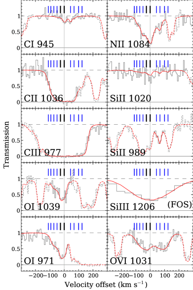
Figure 2: Transitions for the $z=0.56$ sub-DLA in the COS and FOS UV spectra. The smooth red line shows Voigt profile models of the data. Absorption that is not due to the named transition in each panel (usually from H₂) is shown by dashed lines. Tick marks show the component positions from Figure 1, dark ticks show components that have associated H₂ absorption. All transitions are covered by the COS spectra, apart from Si iii, which is covered by the lower resolution FOS spectrum.

Figure 3: Constraints on $N_{\textsc{H\,i}}$ from the Ly$\alpha$ transition. The histogram shows the data, the dashed line the continuum, and the lower green points the residuals as defined in the caption of Figure 1. The thick red solid curve shows the best-fitting $N_{\textsc{H\,i}}$ $=10^{19.5}$ cm^-2 for a single component with $b=20$ km s^-1, and the thinner upper and lower solid curves show $N_{\textsc{H\,i}}$ $=10^{19.3}$ and $10^{19.7}$ cm^-2.

3.4 H₂ velocity structure

We measure H₂ transitions from the $J=0-3$ rotational levels, with upper limits on $J=4$ and $5$. The asymmetric profiles for many of the H₂ lines suggest there is more than one absorbing component. We were also unable to successfully fit the equivalent widths of the transitions using a curve of growth analysis with a single component. Therefore we fitted two H₂ components, with redshifts close to those of the two central strong metal components at $-26$ km s^-1 and $0$ km s^-1 (components 5 and 6 in Table 3). These are clearly separated in the resolution $\sim 6$ km s^-1 HIRES spectra, but blended at the instrumental line profile of COS. However, the large number of transitions over a range of oscillator strengths allow us to constrain velocity structure below the instrumental resolution. As it is not uncommon for H₂ to be significantly offset from the strongest metal absorption – indeed, in Section 5.4 we show that the H₂ is probably produced in a different environment to most of the metal lines – we allow the redshifts of each H₂ component to vary in our fitting procedure.

We experimented with fitting the two components using vpfit, and found there were large degeneracies between the Doppler $b$ parameter and column density. One way to robustly explore the $b$-$N$-$z$ parameter space for the two components is to generate large grids of likelihood values as a function of the fitted parameters over plausible regions of parameter space. However, in our case this proved to be prohibitively expensive computationally. Instead we used a Monte-Carlo Markov Chain (MCMC) technique to sample parameter space. This samples parameter values in proportion to the likelihood value at any point in parameter space. Thus from a set of initial parameter positions, a ‘chain’ of parameter values is generated by a stochastic walk through parameter space with distributions approximating the Bayesian posterior probability for each parameter.

We generated posterior parameter distributions using the package Emcee (The MCMC Hammer, Foreman-Mackey et al., 2012). We fitted for each component’s redshift and $b$ parameter, and for the column density of each rotational level using the 56 transitions shown in Figure 4. All transitions for a component were constrained to have the same $b$ value, which is generally observed to be the case in local sites of H₂ absorption for at least $J$ levels $<3$ (Spitzer et al., 1974). Fitting transitions from each rotational level individually also gives $b$ parameters consistent with a single value. Even after correcting the wavelength scale, residual wavelength shifts of $\sim 1$ km s^-1 remain, so we also allowed a small wavelength shift for each fitted region. Thus we fit for 8 column densities, two redshifts, two $b$ parameters, and one wavelength offset for each of the 56 regions resulting in a total of 68 parameters.

Table 5 gives the parameter estimates and $1\sigma$ errors for the velocity offsets (with respect to metal components 5 and 6), $b$ parameters, and H₂ column densities for each rotational level. The $1\sigma$ regions are determined by marginalising over all other parameters and finding the narrowest region that encompasses $68.3$ per cent of the samples. We choose the parameter estimates to be at the centre of these $1\sigma$ regions. The absorption model with the set of parameters that maximises the likelihood is shown in Figure 4.

$J$	$\log_{10}N$ (cm-2)	$b$ (km s-1)	$\delta v$ (km s-1)
	Component 5
0	$16.17\pm 0.25$	$6.7\pm 0.6$	$3.5\pm 0.6$
1	$17.05\pm 0.28$
2	$16.19\pm 0.19$
3	$15.77\pm 0.12$
4	$<14.5$
5	$<14.5$
	Component 6
0	$15.63\pm 0.39$	$4.3\pm 0.7$	$4.3\pm 0.7$
1	$16.42\pm 0.40$
2	$15.65\pm 0.25$
3	$15.47\pm 0.18$
4	$<14.5$
5	$<14.3$

Table 5: Column densities, $b$ values and velocity offsets for the two components showing H₂ based on Monte Carlo Markov Chain fitting. Errors are $1\sigma$ and the $J=5$ & 6 values are $5\sigma$ upper limits. The velocity offsets are from the redshifts of metal components 5 and 6, given in Table 3.

Figure 4: The H₂ absorption model generated using parameters that maximise the likelihood of the data. The histogram shows the flux divided by the continuum (the darker portions were used to calculate the likelihood), the smooth curves show the model. The residuals – (data - model) / $1\sigma$ – are shown centred on $-0.25$, scaled such that the light gray lines above and below $-0.25$ are the $\pm 1\sigma$ range. A two component model with a single $b$-parameter for each component and redshifts corresponding to components 5 & 6 in Table 3 reproduces the data well.

4 Absorption system properties

4.1 Metallicity

The metallicity, $Z$, can be estimated from an element X using the log of the ratio of the abundance of element X in the absorber, $N_{\textrm{X}}/N_{\textrm{H}}$, to the solar abundance

$$[\mathrm{X}/\mathrm{H}]\equiv\log_{10}\frac{(N_{\textrm{X}}/N_{\textrm{H}})_{\mathrm{obs}}}{(N_{\textrm{X}}/N_{\textrm{H}})_{\sun}}.$$ (1)

Due to a charge transfer between O and H we expect the ratio of the number densities $n_{\rm OI}/n_{\rm O}$ and $n_{\rm HI}/n_{\rm H}$ to be the same (Field & Steigman, 1971), provided the majority of O is in the form of O i and O ii. In the presence of many high energy ionising photons, this is no longer true due to different absorbing cross sections of O i and H i (see Prochter et al., 2010), but the absence of Si iv argues against a hard radiation field for this system, and the best fitting Cloudy models do not predict significant amounts of O in higher ionisation states (O vi is seen, but we argue this occurs in a hotter, collisionally-ionised phase). Oxygen also shows little depletion ($<0.3$ dex) onto dust grains across a range of environments in the ISM of the Milky Way (Jenkins, 2009), so should provide a good estimate of the metallicity.

We find [O i/H i] $=-0.72\pm 0.32$, or $\sim 0.19\,Z_{\odot}$. For the photoionisation analysis in Section 4.5 we assume the metallicity is the same across the entire complex. In one of the few cases where the metallicity has been measured for individual components in a single absorption system, metallicity differences of a factor of ten have been observed (Prochter et al., 2010). However, given that the dispersion in $N_{\textrm{\hbox{{\rm Mg}{\sc\,ii}}}}/N_{\textrm{\hbox{{\rm Fe}{\sc\,ii}}}}$ across the system is not excessively large (the largest log difference between components is $0.38$), the assumption of a constant metallicity seems reasonable. In particular, the two components with H₂ do not show significantly different ion abundance ratios compared to the entire system.

4.2 Dust

Noterdaeme et al. (2008) have found a correlation between the presence of dust and the likelihood of observing H₂ in DLAs, consistent with the main formation mechanism for H₂ being on the surface of dust grains. We can measure the dust content by comparing elements known to deplete strongly onto dust grains (Fe, Mg) to those with low depletion (O). We assume negligible ionisation corrections, but applying corrections from the best-fitting Cloudy model in Section 4.5 does not change our conclusions. We find [Fe/O] $=-0.25^{+0.21}_{-0.29}$ and [Mg/O] $=-0.38\pm 0.28$ for the entire system, indicating mild dust depletion. If we also assume solar abundance ratios we can estimate the dust-to-gas ratio normalised by the value in the solar neighbourhood as

$$\kappa=10^{\mathrm{[X/H]}}(1-10^{\mathrm{[Fe/X]}})\,,$$ (2)

where X is an element that does not deplete strongly onto dust (for a derivation of this expression see the appendix of Wolfe et al., 2003). Using oxygen gives $\log_{10}\kappa<-0.44$, compatible with values found in other higher redshift systems showing H₂ (Ledoux et al., 2003).

4.3 Temperature constraints from line widths

The linewidths of absorption components in the HIRES spectra can be used to constrain the temperature of the gas using the relation $b=\sqrt{2kT/m}$, where $m$ is the mass of the ion and $T$ is the temperature. This constraint is an upper limit, as there can be large-scale turbulent motions in addition to thermal broadening, or the line may not be resolved. Indeed, we fitted each component in Mg ii, Fe ii, and Ca ii with a single $b$ parameter value across all three transitions, consistent with turbulent broadening dominating over thermal broadening. Due to the relatively large masses for these elements, only component 2 gives a constraining upper limit of $6\,000$ K, typical of temperatures in the warm neutral medium in the Milky Way ISM. The H₂ linewidths give upper limits to the temperature of $6\,500$ K and $5\,400$ K for the blue and redder components, but we argue below that the physical conditions in the H₂ gas are probably different to those of the gas where most of the metal lines arise. It is also possible that the H₂ widths are substantially broadened due to turbulent motions.

In conclusion, there are no strong temperature constraints from the linewidths. The relative column densities of the H₂ rotational levels provide an independent measure of the temperature, discussed in the next section.

4.4 H₂ excitation temperature

The ratios of H₂ column densities in different rotational levels can be expressed as excitation temperatures, assuming a Boltzmann distribution across the levels (see Draine, 2011):

$$\frac{N_{J}}{N_{J=0}}=\frac{g_{J}}{g_{J=0}}\exp\left(\frac{-B_{v}J(J+1)}{T_{J0}}\right).$$ (3)

Here $N_{J}$ is the column density for molecules in rotational state $J$, and $g_{J}\equiv(2J+1)(2I+1)$, where $I=0$ if $J$ is odd or 1 if $J$ is even, is the statistical weight of $J$. $B_{v}=85.36$ K and $T_{J0}$ is the excitation temperature from level $J$ to $J=0$.

Fig. 5 shows an excitation diagram for the column densities of the $J=0-3$ transitions for the two H₂ components. If the collisional timescale for the $J=0$ and $J=1$ transitions is much shorter than the photodissociation timescale, which occurs above densities of $\sim 100$ cm^-3 when H₂ is sufficiently self-shielded from dissociating photons, then $T_{10}$ represents the kinetic temperature of the gas (see for example Dalgarno et al., 1973). The $z=0.56$ system is likely only partially self-shielded, but assuming it satisfies these requirements we find a lower limit on $T_{10}$ for each component at $1\sigma$ ($2\sigma$) limits of $123$ K ($64$ K) for component 5 and $77$ K ($37$ K) for component 6. Two illustrative temperatures corresponding to the populations for $J=0-3$ in each component are shown in Fig. 5. However, different physical processes affect the populations of these levels (Jura, 1975b), so it is not expected that a single temperature should match all four levels.

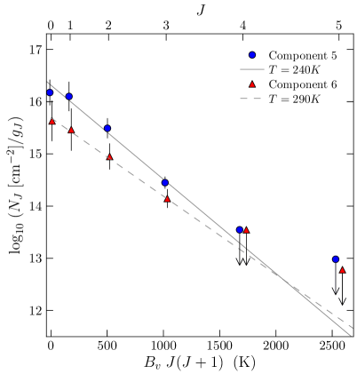
Figure 5: Excitation diagram for the two H₂ components. The error bars show the $1\sigma$ uncertainties. The slope of a line joining each pair of points is inversely proportional to the excitation temperature between those two $J$ levels. An illustrative temperature is shown for each component, but the population levels are not expected to follow a Boltzmann distribution characterised by a single temperature.

4.5 Cloudy modelling

In this section we attempt to generate a simple single-cloud model illuminated by a UV radiation field that can reproduce all the observed column densities. We compare to the total column densities for all components, since the individual component columns are not well constrained for the O i, C i, and Si ii transitions or the saturated transitions (C ii, C iii and Si iii). Given the large range of transitions present with widely differing ionisation energies, it is likely that there are several different phases present, and a single cloud model is unlikely to be able to reproduce all the observed species. Below we find that a single model can reproduce the majority of the low-ionisation metal transitions, but Section 5.4 shows that multiple phases with different densities and temperatures are required to explain all the absorption.

We use models generated with version 8.01 of Cloudy, last described by Ferland et al. (1998), to estimate the physical conditions in the absorption system. All models assume solar abundance ratios, constant gas density, and an absorbing geometry of a thin slab illuminated on one side by an incident radiation field perpendicular to the slab surface. The radiation field includes the cosmic microwave background at the redshift of the absorber. We then compare four scenarios: a cloud in an intergalactic medium-like (IGM) environment, in an ISM-like environment, close to a starburst galaxy, and illuminated by an AGN-dominated spectrum. We chose the AGN-dominated spectrum to estimate the effect of a nearby AGN that may be present in one of the galaxy candidates described in Section 5.3, and to see if a spectrum with more high-energy UV photons can produce the observed O vi column density in addition to that of the low ionisation transitions. The IGM-like model is free of dust with a radiation field given by the UV background spectrum from Haardt & Madau (2012), including contributions from quasars and star-forming galaxies at the redshift of the absorber. It has a radiation field strength at $912$ Å, $J_{\nu,\,\mathrm{IGM}}^{\,912}=6.08\times 10^{-23}$erg s^-1cm^-2Hz^-1sr^-1. The ISM-like models have a radiation field similar to the Galactic ISM ($J_{\nu}^{\,912}\sim 400J_{\nu,\,\mathrm{IGM}}^{\,912}$), which is dominated at UV wavelengths by the spectral shape of hot stars, and a dust grain composition similar to that measured in the ISM. Even though the ISM-like models use solar relative abundances, the gas phase abundance ratios are substantially different from solar due to differential depletion of metals onto grains. The starburst Cloudy models assume the absorbing cloud is 10 kpc from the galaxy and an escape fraction for UV light of 3 per cent, in addition to the IGM-like radiation field described above, without dust grains. They have $J_{\nu}^{\,912}\sim 2700J_{\nu,\,\mathrm{IGM}}^{\,912}$. The starburst galaxy spectrum used was generated using Starburst99 (Leitherer et al., 1999) for a star formation rate of $20$ M_☉ yr^-1. The AGN models use the default tabulated AGN spectrum from Cloudy with a normalisation $J_{\nu}^{\,912}\sim 3000J_{\nu,\,\mathrm{IGM}}^{\,912}$ and do not include dust grains.

For each scenario we generate a grid of models for a range of ionisation parameters, metallicities and total $N_{\textsc{H\,i}}$. We estimate the ionisation parameter $U$, defined as the ratio of the densities of ionising photons to hydrogen atoms, using the observed total column density ratios $N_{\textrm{\hbox{{\rm Mg}{\sc\,i}}}}/N_{\textrm{\hbox{{\rm Mg}{\sc\,ii}}}}$, $N_{\textrm{\hbox{{\rm N}{\sc\,i}}}}/N_{\textrm{\hbox{{\rm N}{\sc\,ii}}}}$, and $N_{\textrm{\hbox{{\rm Si}{\sc\,ii}}}}/N_{\textrm{\hbox{{\rm Si}{\sc\,iii}}}}$. Using ratios of ionisation states for the same element avoids any effects that might alter the column densities of ions for different elements in different ways, such as non-solar abundance ratios or differential dust depletion. We generate the likelihood of each parameter ($U$, $Z$ and $N_{\textsc{H\,i}}$) for the grid of models based on the observed ratios, and include a Gaussian prior on the metallicity centred on the [O i/H i] metallicity measurement with width $\sigma$ equal to the $1\sigma$ uncertainty on the metallicity. For all three scenarios, only a relatively narrow range of $U$ values correctly reproduces the observed ratios. The likelihoods are only weakly dependent on the total $N_{\textsc{H\,i}}$; we assume $N_{\textsc{H\,i}}$ $=10^{19.5}$ cm^-2, which results in models that best reproduce the observed metal column densities.

Once we have found the most likely $U$ value, we compare the predicted column densities to the observed transitions with measurements or limits, and assess which scenario reproduces the observations best. We first compare to the AGN models. These are the only models with a hard enough spectrum to produce sufficient $N_{\textrm{\hbox{{\rm O}{\sc\,vi}}}}$ to match the observed value. However, at the same time they overpredict the amount of Si iv, Fe ii, Mg i and Mg ii by one or more orders of magnitude. Thus it is more likely the O vi arises in a collisionally-ionised phase separate from the low-ionisation transitions, as is observed in other systems (for example Fox et al., 2007; Ribaudo et al., 2011), and we do not compare to the high-ionisation species (Si iv, O vi) for the remaining models.

From the mild depletions measured in Section 4.2, we already expect that the ISM-like case will not match the observed abundances. The most likely model does indeed underpredict the Fe ii abundance by more than an order of magnitude, and Ca ii by many orders of magnitude, as both are expected to be heavily depleted onto dust grains. This confirms that the depletion pattern in the $z=0.56$ sub-DLA is different from that in the Milky Way ISM. This model also underpredicts C i. The starburst scenario fails to reproduce the observed $N_{\textrm{\hbox{{\rm N}{\sc\,i}}}}/N_{\textrm{\hbox{{\rm N}{\sc\,ii}}}}$, and also severely underpredicts Ca ii, Fe ii and C i. The IGM-like model gives the best fit to the observed data, and its predictions along with observed column densities are shown in Figures 6 & 7. Figure 6 shows that column densities for O i, Mg i, Mg ii, Fe ii, N i and N ii are reasonably well matched. The remaining small deviations from the predictions could be due to a slightly different incident UV continuum from the one assumed, or enhanced or depleted elemental abundances relative to the solar values assumed. For example, $0.2$ dex less $N_{\textrm{\hbox{{\rm N}{\sc\,ii}}}}$ is observed than is predicted. This may be due to a nitrogen underabundance, often observed in similar $N_{\textsc{H\,i}}$ systems at low redshifts (for example Battisti et al., 2012) and in DLAs at higher redshifts (Pettini et al., 2002; Prochaska et al., 2002). Figure 7 shows that Si ii, Si iii, C ii and C iii columns are reproduced well. However, there is still $0.5$ dex too little $N_{\textrm{\hbox{{\rm Ca}{\sc\,ii}}}}$ and 1 dex too little $N_{\textrm{\hbox{{\rm C}{\sc\,i}}}}$ predicted. In all three scenarios, we also find that the $N_{\textrm{H}_{2}}$ predicted is more than an order of magnitude below the observed value. In Section 5.4 we suggest a scenario to explain this discrepancy between the models and observations.

We also ran Cloudy models using constant pressure clouds instead of constant density. The motivation for these was to simultaneously include cool, lower density gas at the edge of the cloud, and higher density, cold $\sim 100$ K gas at the core of the cloud where H₂ can survive. In these models we also included contributions from cosmic rays, which can be important for cold molecular regions. Although significant amounts of H₂ can co-exist with many of the metal transitions observed for these models, they still cannot correctly reproduce the Ca ii or C i columns.

Figure 6: Cloudy predictions (lines) and observed column densities (points) for Mg i, Mg ii, N i, N ii, O i and Fe ii for the IGM-like model with $Z=0.13\,Z_{\odot}$. Points are plotted at the most likely $U$ values based on constraints from the $N_{\textrm{\hbox{{\rm Mg}{\sc\,i}}}}/N_{\textrm{\hbox{{\rm Mg}{\sc\,ii}}}}$, $N_{\textrm{\hbox{{\rm N}{\sc\,i}}}}/N_{\textrm{\hbox{{\rm N}{\sc\,ii}}}}$, and $N_{\textrm{\hbox{{\rm Si}{\sc\,ii}}}}/N_{\textrm{\hbox{{\rm Si}{\sc\,iii}}}}$ ratios (Fe ii is offset for clarity). Filled points correspond to solid lines of the same colour, open points to dashed lines. Errors on the column densities are smaller than the marker sizes. Given the uncertainties in the shape of the ionising spectrum and uncertain relative abundances, the predicted column densities are very close to the observed values.

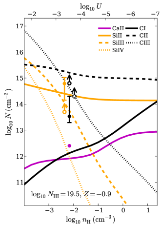
Figure 7: Cloudy predictions (lines) and observed column densities (points) for C i, C ii, C iii, Si ii, Si iii and Ca ii for the IGM-like model with $Z=0.13\,Z_{\odot}$. Points are plotted at the most likely $U$ values based on constraints from the $N_{\textrm{\hbox{{\rm Mg}{\sc\,i}}}}/N_{\textrm{\hbox{{\rm Mg}{\sc\,ii}}}}$, $N_{\textrm{\hbox{{\rm N}{\sc\,i}}}}/N_{\textrm{\hbox{{\rm N}{\sc\,ii}}}}$, and $N_{\textrm{\hbox{{\rm Si}{\sc\,ii}}}}/N_{\textrm{\hbox{{\rm Si}{\sc\,iii}}}}$ ratios (Si and C iii points are offset for clarity). Filled points correspond to solid lines of the same colour, open points to dashed lines, and open points with dotted edges to dotted lines. Where error bars are not shown they are smaller than the marker size. With the exception of C i and Ca ii, the column densities are reproduced well. As discussed in Section 5.4, the excess $N_{\hbox{{\rm C}{\sc\,i}}}$ is likely due to C i being in a self-shielded cold phase where the H₂ and possibly part of the Ca ii resides.

4.6 C ii fine structure absorption

Singly ionised carbon (C⁺) has electronic structure $2s^{2}2s^{2}2p$ where the outer shell has a configuration ²P${}^{\mathrm{o}}_{J}$, and thus fine structure splitting occurs between the $J=1/2$ and $J=3/2$ levels. Transitions from these two ground state levels produce C ii and C ii^∗ absorption respectively.

The ratio of C ii^∗ to C ii column densities has been used to estimate the star formation rate inferred from the cooling rate in DLAs at high redshift (Wolfe et al., 2003). We find an upper limit on C ii^∗ from $\lambda 1036$ of $N_{\textrm{\hbox{{\rm C}{\sc\,ii}${}^{*}$}}}<10^{14.5}$  cm^-2 and $N_{\textrm{\hbox{{\rm C}{\sc\,ii}}}}>10^{14.6}$  cm^-2. Assuming constant $n($C ii^∗)$/n($C ii) over the entire complex, we find the ratio $N_{\textrm{\hbox{{\rm C}{\sc\,ii}${}^{*}$}}}/N_{\textrm{\hbox{{\rm C}{\sc\,ii}}}}<0.8$, consistent with ratios measured in higher redshift DLAs (for example Srianand et al., 2005) and local environments. Following the assumptions described by Morris et al. (1986), we can estimate the electron density $n_{e}$ in cm^-3 using the expression:

$$\frac{N_{\textrm{\hbox{{\rm C}{\sc\,ii}${}^{*}$}}}}{N_{\textrm{\hbox{{\rm C}{\sc\,ii}}}}}=3.9\times 10^{-2}\,n_{e}\,[1+(0.22\frac{n_{p}}{n_{e}})]$$ (4)

We use $n_{p}/n_{e}$ corresponding to the ionised H fraction of $0.70$ from the best-fitting Cloudy ionisation model to find $n_{e}<10$ cm^-3. Using $N_{\textsc{H\,ii}}$ we can estimate the thickness of the absorbing cloud as $N_{\textsc{H\,ii}}$$/n_{e}$. This gives a lower limit on the cloud size of $3$ pc. This limit is not necessarily related to the density or size of the H₂ gas, as we argue in the discussion that most of the C ii is due to a warm ionised phase separate from the H₂.

4.7 Molecular fraction

The molecular mass fraction is estimated by

$$f_{\textrm{H}_{2}}=2N_{\textrm{H}_{2}}/(N_{\textrm{\hbox{{\rm H}{\sc\,i}}}}+2N_{\textrm{H}_{2}}),$$ (5)

assuming most of the hydrogen associated with the H₂ is neutral. In this case, as for many other QSO absorption systems, it is not clear how to divide the total $N_{\textsc{H\,i}}$ measured from the damping wings between different absorbing components, and in principle each $N_{\textrm{H}_{2}}$ component could have a different $f_{\textrm{H}_{2}}$ value. To calculate $f_{\textrm{H}_{2}}$ we use the total $N_{\textrm{H}_{2}}$ from both components and conservatively assume all $N_{\textsc{H\,i}}$ is associated with the H₂, meaning $f_{\textrm{H}_{2}}$ is effectively a lower limit. This gives a molecular fraction of $\log_{10}$ $f_{\textrm{H}_{2}}$ $=-1.93\pm 0.36$. As we discuss in the next section, given the total $N_{\textsc{H\,i}}$, this is an usually high molecular fraction compared to most other higher redshift systems and sightlines in the Local Group. Therefore we may be concerned that a different velocity model to the one we have used permits a much lower $f_{\textrm{H}_{2}}$. To calculate a lower limit on $f_{\textrm{H}_{2}}$ independent of the velocity model, we measure the column density of the lowest oscillator strength transition available for each rotational level ($J=0$, $\lambda 1108.1$; $J=1$, $\lambda 1008.5$; $J=2$, $\lambda 934.1$ and $J=3$, $\lambda 952.3$) using the AOD method. This gives a lower limit of $N_{\textrm{H}_{2}}$$=10^{16.5}$ cm^-2 or $f_{\textrm{H}_{2}}$ $>10^{-3}$, again assuming all of the $N_{\textsc{H\,i}}$ is associated with the $N_{\textrm{H}_{2}}$. This is still a high value relative to local H₂ systems with similar $N_{\textsc{H\,i}}$.

5 Discussion

5.1 Physical conditions in the H₂ cloud

To consider this system in the context of other H₂ detections in absorption, we plot $f_{\textrm{H}_{2}}$ for local and higher redshift H₂ sightlines as a function of the total hydrogen column density and $N_{\textrm{H}_{2}}$ in Figure 8. It is apparent that the $z=0.56$ sub-DLA (solid circle) has an unusually high $f_{\textrm{H}_{2}}$ given its $N_{\textsc{H\,i}}$ compared to sightlines through the plane of the Milky Way (cyan inverted triangles), or through the Magellanic clouds (green squares and red diamonds).

Figure 8: The molecular fraction versus the total $N_{\textrm{H}}$. Compared to measurements in the Magellanic clouds (Tumlinson et al., 2002; Welty et al., 2012), along the disk of the Milky Way (Savage et al., 1977) and in intermediate- (Richter et al., 2003) and high-velocity clouds (Richter et al., 1999), the $z=0.56$ H₂ system has an unusually large $f_{\textrm{H}_{2}}$ for its total H column. The local systems that appear most similar to this absorber are seen along sightlines through the Magellanic Stream (Sembach et al., 2001; Richter et al., 2001). Error bars at the corner of each plot show the typical uncertainties on $f_{\textrm{H}_{2}}$, $N_{\mathrm{tot}}$ and $N_{\textrm{H}_{2}}$. Shading shows the regions in which H₂ cannot be detected for a limit of $N_{\textrm{H}_{2}}$  $\lesssim 10^{14.5}$  cm^-2, a typical threshold for the spectra used for the different surveys. The thin lines at the top right in each panel show analytic models from Krumholz and McKee for two illustrative metallicities. The three thin lines at the lower left are the analytic models described in Section 5.1. H₂ detections in $z>1.5$ QSO absorption systems (from the compilation by Noterdaeme et al. 2008 with additions from Petitjean et al. 2002, Reimers et al. 2003, Noterdaeme et al. 2010, Srianand et al. 2008, 2010, 2012, Tumlinson et al. 2010, Jorgenson et al. 2010 and Guimarães et al. 2012) are also shown.

Before we discuss the likely origin of the $z=0.56$ sub-DLA, we examine the physics underlying the $f_{\textrm{H}_{2}}$ distribution as a function of $N_{\textrm{H}}$ and $N_{\textrm{H}_{2}}$. The left panel shows a clear bimodality in the $f_{\textrm{H}_{2}}$ $-N_{\textrm{H}}$ distribution between high $N_{\textrm{H}}$, high $f_{\textrm{H}_{2}}$ sightlines at the top right, and lower $f_{\textrm{H}_{2}}$ sightlines, generally with much lower $N_{\textrm{H}}$. The right panel shows this is actually a bimodality between $N_{\textrm{H}_{2}}$ values $\lesssim 10^{16}$ cm^-2 and $\gtrsim 10^{18}$ cm^-2. This can be understood as the onset of H₂ self-shielding against UV dissociating photons (for example Hirashita & Ferrara, 2005; Gillmon et al., 2006). An analytic approximation from Draine & Bertoldi (1996) shows that $>97$ per cent of H₂-dissociating photons are blocked by self-shielding once $N_{\textrm{H}_{2}}$ $\sim 10^{16}$ cm^-2. Once H₂ becomes self-shielded, the dissociation rate drops and H₂ accumulates rapidly to the formation-destruction equilibrium value predicted by the models by McKee & Krumholz (2010). These models are shown at the top right in each panel for two metallicities; solar and $Z=0.2Z_{\odot}$, the metallicity of the SMC. They were calculated using equations 4, 5, 7 and 8 from Kuhlen et al. (2012) and assume the ISM is in a two phase equilibrium between a cold neutral medium and a warm neutral medium (for example Wolfire et al., 1995). The solar metallicity model reproduces the mean $f_{\textrm{H}_{2}}$ for the Milky Way sightlines through shielded H₂ regions reasonably well, although Welty et al. (2012) point out that these models overpredict the $N_{\textrm{H}}$ at which this transition occurs.

The $N_{\textrm{H}}$ at which there is sufficient shielding from the UV field to form large amounts of H₂ varies depending on the dust to gas ratio, the strength of the UV field, and the H₂ linewidth, so the $N_{\textrm{H}}$ at which the transition from optically thin to optically thick occurs can change from sightline to sightline. In the plane of the MW disk, the transition from low to higher $f_{\textrm{H}_{2}}$ takes place around $N_{\textrm{H}}=10^{20.5}-10^{21}\,$cm^-2. It occurs at higher $N_{\textrm{H}}$ in the LMC and SMC, both because their lower metallicities ($0.5$ and $0.2Z_{\odot}$ respectively, see the appendices from Welty et al., 1997, 1999) result in a lower H₂ formation rate on grains, and due to an increased UV field compared to the Milky Way (Tumlinson et al., 2002). Gillmon et al. (2006) have also shown the large variation in $f_{\textrm{H}_{2}}$ along different sightlines implies that each sightline intersects a small number of molecule-bearing clouds.

In addition to comparing to the two-phase equilibrium models of McKee & Krumholz, we can compare to simple analytic models that apply to diffuse H₂ in the partially shielded regimes. Following the Appendix from Jorgenson et al. (2010), the dissociation rate in s^-1 due to photons with energies corresponding to the Lyman-Werner bands is given by

$$R_{\textrm{diss}}=1.1\times 10^{8}\,4\pi J_{\nu}^{\textrm{LW}}\,S_{\textrm{shield}},$$ (6)

where $J_{\nu}^{\textrm{LW}}$ is the strength of the incident radiation field in erg s^-1cm^-2Hz^-1sr^-1 at 1000 Å, and $1-S_{\textrm{shield}}$ is the fraction of Lyman-Werner photons processed by dust or scattered due to H₂ shielding, which can be calculated using the analytic expressions from Draine & Bertoldi (1996) and Hirashita & Ferrara (2005). In formation-dissociation equilibrium, the molecular fraction can be approximated by

$$f_{\textrm{H}_{2}}=2\,\frac{\kappa\mathcal{R}n_{\textrm{\hbox{{\rm H}{\sc\,i}}}}}{R_{\textrm{diss}}},$$ (7)

where $\mathcal{R}$ is the formation rate of H₂ on dust grains in cm³ s^-1, $n_{\textrm{\hbox{{\rm H}{\sc\,i}}}}$ is the H i particle density in cm^-3 and $\kappa$ is the dust to gas ratio relative to that in the solar neighbourhood as defined in Section 4.2. Note that the formation rate term used by Hirashita & Ferrara (2005), $R_{\mathrm{dust}}$, is equal to $\kappa\mathcal{R}$. Rearranging these expressions, we can estimate the particle density in the cloud as:

$$n_{\textrm{\hbox{{\rm H}{\sc\,i}}}}=74\,\mbox{cm${}^{-3}$}\kappa^{-1}\left(\frac{\mathcal{R}}{\mathcal{R}_{\mathrm{SN}}}\right)^{-1}\left(\frac{f_{\textrm{H}_{2}}}{0.01}\right)\left(\frac{J_{\nu}^{\textrm{LW}}}{J_{\nu,\,\mathrm{SN}}^{\textrm{LW}}}\right)\left(\frac{S_{\mathrm{shield}}}{0.01}\right),$$ (8)

where $J_{\nu,\,\mathrm{SN}}^{\textrm{LW}}=3.2\times 10^{-20}$ erg s^-1 cm^-2 Hz^-1 sr^-1 and $\mathcal{R}_{\mathrm{SN}}=3\times 10^{-17}$ cm³ s^-1 are typical values measured in the solar neighbourhood (Habing, 1968; Jura, 1974).

The three curves at the lower left of each panel in Figure 8 show the molecular fractions estimated with equation (7) for illustrative combinations of $\kappa\mathcal{R}n_{\textrm{\hbox{{\rm H}{\sc\,i}}}}/R_{\textrm{diss}}$. The upper curve and middle curves each have $n_{\textrm{\hbox{{\rm H}{\sc\,i}}}}=10$ cm^-3 with $\kappa=0.04$, $0.1\mathcal{R}_{\mathrm{SN}}$, $10J_{\nu,\,\mathrm{SN}}^{\textrm{LW}}$ and $\kappa=1$, $0.33\mathcal{R}_{\mathrm{SN}}$, $2J_{\nu,\,\mathrm{SN}}^{\textrm{LW}}$ respectively. The lower curve has $\kappa=0.04$, $n_{\textrm{\hbox{{\rm H}{\sc\,i}}}}=5$ cm^-3, $\mathcal{R}_{\mathrm{SN}}$ and $0.01J_{\nu,\,\mathrm{SN}}^{\textrm{LW}}$. This lower curve has qualitatively different behaviour from the upper two curves, because at such low molecular fractions, dust shielding from dissociating photons becomes important before H₂ self-shielding. Therefore the observed variation in $f_{\textrm{H}_{2}}$ can be explained by reasonable variations in the combination of UV field strength, particle density and H₂ dust formation rate. If the $z=0.56$ system is in H₂ formation-dissociation equilibrium, the combination of low $N_{\textsc{H\,i}}$ and high molecular fraction suggests that it is either in a weaker UV field, has an increased H₂ formation rate, a higher $n_{\rm H}$ compared to the solar neighbourhood, or some combination of these three. We can use limits on the column densities of the $J=4$ and $5$ levels to put upper limits on $J_{\nu}^{\textrm{LW}}$ (Jura, 1975b). These upper limits are not very stringent, however, due to weak limits on the column densities, and constrain $J_{\nu}^{\textrm{LW}}\lesssim 10^{-18}$ erg s^-1cm^-2Hz^-1sr^-1. This is consistent with the different UV background values assumed in the Cloudy models, which range from $\sim 10^{-22}$ for the IGM-like scenario to $\sim 10^{-20}$ erg s^-1cm^-2Hz^-1sr^-1 for the ISM-like scenario.

Using $f_{\textrm{H}_{2}}$ and $N_{\textrm{H}_{2}}$ measured in the $z=0.56$ sub-DLA, the measured metallicity and equation (8), we find densities of $\sim 1-4$ cm^-3 for a UV background incident radiation field, and $\sim 70-480$ cm^-3 for a Milky Way ISM-like radiation field. The lower density range corresponds to cloud thicknesses of $\sim 3-10$ pc, the high density range to $\sim 0.002-0.15$ pc. The only direct measurement of the size of a redshifted H₂ absorber is by Balashev et al. (2011), through partial covering of a background QSO broad line region. They find the region producing H₂ is $\sim 0.15$ pc and its surrounding neutral envelope $\sim 8$ pc, both of which are consistent with our size estimates. The upper end of our density range is consistent with values measured for higher redshift H₂ systems using C i fine structure transitions, but would result in extremely small cloud sizes.

The low total column density of the $z=0.56$ system suggests that it does not pass through the ISM of a galaxy. Returning to Figure. 8, we see that local systems with similarly low total $N_{\textrm{H}}$ and almost as high $f_{\textrm{H}_{2}}$ are sightlines through a high velocity cloud (Richter et al., 1999) and the Magellanic Stream (Sembach et al., 2001; Richter et al., 2001). These clouds have sub-solar metallicities ($0.3-0.5$ solar), and are most likely tidally stripped from the Magellanic Clouds (for the Magellanic Stream) or the Milky Way. Sembach et al. (2001) estimate the density of the H₂-bearing cloud they observed in the Magellanic Stream to be $0.3-3$ cm^-3 with a photoionisation rate at least a factor of 10 smaller than the Milky Way ISM value. The H₂ formation timescale for these low densities is around $1$ Gyr, a large fraction of the estimated lifetime of the Magellanic Stream (for example Besla et al., 2010). Therefore they favour a scenario where H₂ is not formed in place, but has survived the tidal stripping process and persists due to a combination of self-shielding and the lower ambient UV field compared to the LMC ISM. Such a scenario could also be responsible for the $z=0.56$ absorber.

5.2 Comparison to higher-redshift H₂ absorbers

Unlike the local sightlines, there is no clear bimodality in the $f_{\textrm{H}_{2}}$ – $N_{\textrm{H}}$ distribution for higher-$z$ H₂ systems. This could be due to each higher-$z$ absorber being comprised of several clouds, or to a much wider range of incident UV and H₂ formation rates, both of which may smooth away an underlying distribution.

The three high-$z$ systems with $f_{\textrm{H}_{2}}$ and $N_{\textrm{H}}$ most similar to this system are those described by Petitjean et al. (2002) (at $z=1.973$ towards Q0013-0029 with $\hbox{$N_{\textsc{H\,i}}$}\leq 10^{19.4}$ cm^-2, $\hbox{$f_{\textrm{H}_{2}}$}=10^{-2.63}$), Reimers et al. (2003) ($z=1.51$ towards HE0515$-$4414 with $\hbox{$N_{\textsc{H\,i}}$}=10^{19.88}\,$cm^-2, $\hbox{$f_{\textrm{H}_{2}}$}=10^{-2.64}$), and Tumlinson et al. (2010) and Milutinovic et al. (2010) ($z=2.059$ towards Q2123$-$0500 with $\hbox{$N_{\textsc{H\,i}}$}=10^{19.18}\,$cm^-2, $\hbox{$f_{\textrm{H}_{2}}$}=10^{-1.54}$). The $z=1.973$ system is a sub-DLA component that is highly depleted to the same extent as is observed for cool gas in the Milky Way. It has a solar metallicity and the gas pressure is even higher than is typically measured in Milky Way ISM. The $z=1.51$ system has a metallicity of 0.3 solar, and dust to gas ratio of $0.89\pm 0.19$ relative to solar. It also shows evidence of a higher photodissociation rate than is seen locally. The final sub-DLA at $z=2.059$ has a metallicity of 0.5 solar, and HD absorption is observed in addition to H₂. It exhibits a multi-phase medium of cold and warm gas, similar to the system we have presented is this paper. Unfortunately none of these absorbers have associated imaging to suggest a typical impact parameter of any nearby galaxy producing the absorption.

Therefore, the three higher redshift systems showing a similarly high $f_{\textrm{H}_{2}}$ and low $N_{\textsc{H\,i}}$ tend to have larger metallicities and dust to gas ratios than the $z=0.56$ absorber. However, it is possible that the components producing H₂ in the $z=0.56$ system have a higher metallicity and dust-to-gas ratio than that averaged over the whole absorber.

5.3 Connection to galaxies

The $K$ band imaging around Q 0107$-$0232 has a seeing FWHM of 0.8″, and shows two possible galaxy candidates less than 1.2″ from the QSO sightline. Figure 9 shows a $5$″$\times 5$″ region centred on the QSO. The QSO image has been subtracted using the point spread function of a nearby star. The two galaxy candidates are seen to the North-West (G1) and South-West (G2). Assuming they are at the redshift of the absorber, they have luminosities of $0.7L^{*}$ (G1) and $2L^{*}$ (G2), and impact parameters of $10$ kpc (G1) and $11$ kpc (G2), both smaller than the median impact parameter of $33$ kpc for galaxies associated with sub-DLAs found by Rao et al. (2011). Therefore it is likely that at least one is associated with the absorber, on scales typical of the separations between the Milky Way and high-velocity clouds (10-60 kpc, see Putman et al. 2012 and the references therein).

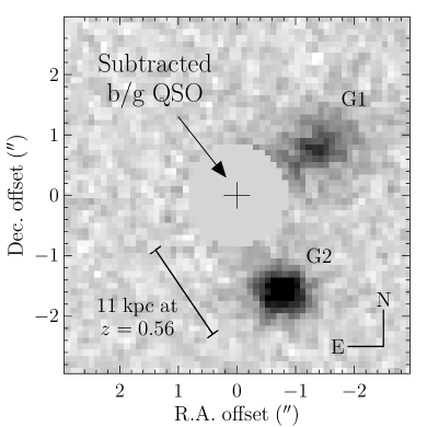
Figure 9: A K-band image of the QSO showing two nearby galaxy candidates, G1 and G2. The QSO image has been subtracted using the point spread function of a nearby star. The region near the centre of the QSO still shows significant residuals and has been greyed out. If G1 and G2 are at the redshift of the QSO then they have impact parameters of $10$ kpc and $11$ kpc, and luminosities of $0.7L^{*}$ and $2L^{*}$ respectively.

5.4 Three different gas phases in the sub-DLA

Figures 6 & 7 show the total hydrogen particle density for the majority of metals observed in this system corresponding to the ionisation parameter, assuming the normalisations of the incident radiation fields are correct. The most likely model corresponds to hydrogen densities from $10^{-3}$ to $10^{-2}$ cm^-3. Even assuming a factor of ten uncertainty in the radiation field strength, this is much lower than the typical densities where H₂ is seen in both our galaxy and in other H₂-bearing DLAs ($n_{\rm H}=10-100$ cm^-3). This is confirmed by our Cloudy modelling, which shows that there is no single cloud model that can simultaneously reproduce both the C i and H₂ column densities, in addition to those of the other low-ionisation metal transitions. Therefore the gas traced by most of the metal absorption is probably in a different environment to that in which the H₂ resides. This is also likely the cause of the excess $N_{\textrm{\hbox{{\rm C}{\sc\,i}}}}$ over that predicted by the Cloudy models. C i is often seen in dense components showing H₂ (for example Srianand et al., 2005) and can have extremely narrow linewidths corresponding to temperatures of $\sim 100$ K (Jorgenson et al., 2009; Carswell et al., 2011), indicating it occurs in the same environment as H₂. Thus most of the C i and some Ca ii may be from a high density region co-spatial with the H₂.

As discussed in Section 4.5, the presence of O vi is unlikely to be explained by photoionisation by a hard UV field. At the metallicity of the absorber ($\sim 0.1$ solar), significant O vi is only produced via collisional ionisation for temperatures larger than $10^{5}$ K, even in non-equilibrium cases (Gnat & Sternberg, 2007). Thus it is likely a hotter medium than that producing the H₂ and metal lines is also present.

We conclude that the absorption is due to gas in three phases: a photoionised medium at $\sim 10^{4}$ K in which most of the metal transitions we see are produced, a cold neutral medium at $\sim 100$ K where the H₂ and C i absorption occurs, and a hotter phase where O vi is produced. The H i column is likely split between the two cooler phases. A similar multi-phase environment is also seen in other higher redshift sub-DLAs that show molecular absorption (Milutinovic et al., 2010).

The Magellanic Stream and many other HVCs comprise $10^{4}$ K ionised gas that is seen in H$\alpha$ emission, T $>10^{5}$ K hot gas producing O vi absorption, and they can also contain cold neutral gas with H₂ (Sembach et al., 2003; Fox et al., 2010). Taken together, the existence of these three phases, the high molecular fraction with a low total column density, and the proximity of a possible $\sim L^{*}$ galaxy suggest the $z=0.56$ absorber is due to a tidally stripped feature analogous to the Magellanic Stream.

5.5 Incidence rate of H₂ in low redshift sub-DLAs

Due to the need for bright targets observable with space-based UV spectroscopy and their low incidence rate, very few DLAs and sub-DLAs have been found at low redshift. Until recently only $\sim 10$ DLAs at redshifts $<1$ were known, and only a handful of these have coverage of H₂ Lyman-Werner bands. With the availability of COS, the number of such systems is being increased dramatically, and due to its far UV wavelength coverage the presence of H₂ can be easily detected.

Battisti et al. (2012) present a sample of $2$ DLAs and $6$ sub-DLAs at $z<0.35$, serendipitously discovered along sightlines as part of a large COS program. Like the sub-DLA presented here, they were not pre-selected by the strength of their metal lines or other properties that might influence the likelihood of detecting molecules. Interestingly, they also discovered a sub-damped system with H₂ absorption at $z=0.2477$. Taking this sample together with the system in this paper and assuming binomial statistics, we find the expected incidence rate of DLAs and sub-DLAs showing molecular hydrogen at $N_{\textrm{H}_{2}}$ $\gtrsim 10^{14}$ cm^-2 at low redshift to be $2/9=22$ per cent (with a $95$ per cent confidence level lower limit of $4$ per cent), rising to $33$ ($5$) per cent if we consider only the sub-damped systems with $N_{\textsc{H\,i}}$ $<10^{20}$ cm^-2. This is a surprisingly large fraction given that sub-DLAs are often found to be highly ionised absorbers with $\lesssim 10$ per cent of their hydrogen in the form of H i.

If we think that the absorption cross section for H₂ is dominated by cold gas associated with Local Group-type systems (the Magellanic Stream for example), then this may be consistent with this high incidence rate. Richter (2012) shows that one can explain 30-100 per cent of the observed incidence rate of systems with $N_{\textsc{H\,i}}$ $>10^{17.5}$  cm^-2 as intermediate- and high-velocity clouds distributed around galaxies with H i masses between $10^{8.5}$ and $10^{10}$ M_☉ in a similar way as is seen around M31 and the Milky Way. As discussed in the previous section, some HVCs also show relatively high molecular fractions, and in terms of $N_{\textsc{H\,i}}$ and $f_{\textrm{H}_{2}}$ HVCs are the local systems most analogous to the system analysed in this paper.

It would be interesting to perform a systematic search for H₂ in further $10^{19}$ cm^-2 $<$ $N_{\textsc{H\,i}}$ $<10^{20.3}$ cm^-2 sub-DLAs at both high and low redshifts that have metal absorption consistent with a cool, dusty environment. Sub-DLAs tend to have both higher metallicities and larger velocity widths than DLAs, and H₂ is more likely to be found in DLAs with both these characteristics (Noterdaeme et al., 2008).

5.6 Evolution in $f_{\textrm{H}_{2}}$

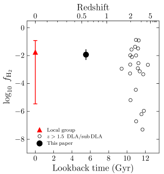
Figure 10: The molecular mass fraction as a function of lookback time for sites where H₂ absorption has been detected. The Local Group point is a median for all values from the plane of the Milky Way (Savage et al., 1977), the LMC and SMC (Welty et al., 2012). The error bars show the 10th and 90th percentile level. There is no evidence for evolution in $f_{\textrm{H}_{2}}$, but the number of measurements at $z>0$ is small.

We plot the $f_{\textrm{H}_{2}}$ values as a function of cosmic time in Figure 10. There is no evidence for evolution in $f_{\textrm{H}_{2}}$, though more measurements are needed, particularly at intermediate redshifts, given the large scatter in $f_{\textrm{H}_{2}}$ seen along both local sightlines in the Milky Way halo and in higher $z$ DLAs.

6 Summary

We have analysed a sub-damped Ly$\alpha$ system with $N_{\textsc{H\,i}}$$=10^{19.5\pm 0.2}$ cm^-2 at $z=0.56$ that shows associated molecular hydrogen absorption in the Lyman and Werner bands. Using velocity components determined from a high resolution spectrum covering metal transitions falling in the optical, we fit a two-component model to the H₂ absorption and find a lower limit to the molecular fraction of $\log_{10}\hbox{$f_{\textrm{H}_{2}}$}=-1.93\pm 0.36$, and a lower limit independent of the assumed velocity structure of $f_{\textrm{H}_{2}}$ $>10^{-3}$. This is higher than other sightlines with similar $N_{\textsc{H\,i}}$ where H₂ has been measured in the Milky Way halo. We find a metallicity for the cloud $\log_{10}Z=-0.72\pm 0.32$, or $0.19^{+0.21}_{-0.10}$ solar. The dust-to-gas ratio relative to the solar neighbourhood is $\log_{10}\kappa<-0.44$, or $\kappa<0.36$.

We modeled the observed transitions using Cloudy and were unable to find a single solution that can simultaneously reproduce all the observed transitions. However, a model for the absorber of a $10^{4}$ K cloud illuminated by a radiation field dominated by the UV background can broadly reproduce all the observed column densities apart from those of H₂, C i, and O vi. We conclude that there are three phases in the absorber; a $T\sim 100$ K phase where the C i and H₂ arise, a $T\sim 10^{4}$ K phase where the low-ionisation metal absorption occurs, and a hotter, collisionally ionised phase associated with O vi.

Using simple models of H₂ formation-dissociation equilibrium, we calculate densities for the H₂ absorbing region from $\sim 1-4$ cm^-3 to $\sim 70-480$ cm^-3, depending on the incident strength of the radiation field. The lower density range corresponds to cloud thicknesses of $\sim 3-10$ pc, the high density range to $\sim 0.002-0.15$ pc. Given the $N_{\textsc{H\,i}}$, the presence of a three phase medium, the molecular fraction, metallicity and two galaxy candidates near the QSO sightline with impact parameters of $\sim 10$ kpc, we conclude this system may be a tidally stripped feature similar to the Magellanic Stream.

Finally, we remark that of the seven sub-DLAs observed at $z<0.7$ for which there is the possibility to detect $N_{\textrm{H}_{2}}$ $\gtrsim 10^{14.5}$ cm^-2, two H₂ detections were found. A survey for H₂ in low-redshift sub-damped systems could be a fruitful way to measure the physical conditions giving rise to these absorbers.

We acknowledge helpful correspondence with Jason Tumlinson and thank Andrew Fox, Joe Hennawi, Mark Krumholz, Kate Rubin, Karin Sandstrom and Todd Tripp for illuminating conversations, and Dan Welty for comments on an earlier version of this paper. Gabor Worseck kindly helped us to obtain the HIRES spectrum of Q 0107$-$0232. We thank the anonymous referee for comments that helped improve the paper.

Some of the data presented here were taken at the W.M. Keck Observatory, which is operated as a scientific partnership among the California Institute of Technology, the University of California and the National Aeronautics and Space Administration. The Observatory was made possible by the generous financial support of the W.M. Keck Foundation. This analysis made use of observations from the NASA/ESA Hubble Space Telescope, obtained at the Space Telescope Science Institute, which is operated by the Association of Universities for Research in Astronomy, Inc., under NASA contract NAS 5-26555 (program 11585) and of observations collected at the European Organisation for Astronomical Research in the Southern Hemisphere, Chile (program 383.A-0402).

The authors wish to recognize and acknowledge the significant cultural role and reverence that the summit of Mauna Kea has always had within the indigenous Hawaiian community. We are most fortunate to have the opportunity to conduct observations from this mountain.

N.T. acknowledges grant support by CONICYT, Chile (PFCHA/Doctorado al Extranjero 1^a Convocatoria, 72090883). Most of the programs particular to this analysis were written using the NumPy and SciPy packages (http://www.scipy.org), and plots were produced using Matplotlib (Hunter, 2007, http://www.matplotlib.sourceforge.net).

Appendix A Correcting for wavelength shifts in the COS exposures.

When combining the COS exposures, we found there were shifts of $\sim 20$ km s^-1 in the wavelength solution between exposures taken using different central wavelength settings. Table 6 gives the shifts that must be applied to bring our G160M exposures with central wavelength settings 1589 and 1627 Å to a common wavelength scale. Table 7 gives the further $\sim 10$ km s^-1 shifts that were required to give an internally consistent wavelength solution based on the expected positions of H₂ absorption features.

	Valid	Apply to
Segment	$\lambda$ range (Å)	$\lambda$ setting	$\alpha$	$\beta$
FUVA	$1600$ – $1800$	1627	$1.233\times 10^{-3}$	$-$2.115
FUVB	$1425$ – $1600$	1589	$-0.952\times 10^{-3}$	1.468

Table 6: Wavelength shifts required to bring COS G160M exposures with central wavelength settings 1589 and 1627 Å on to a common wavelength scale. The shift $\Delta\lambda$ that must be added to a wavelength $\lambda$ is given by $\Delta\lambda=\alpha\lambda+\beta$. The FUVA shift is applied to the 1627 central wavelength setting, and the FUVB shift is applied to the 1589 setting.

$\lambda$ (Å)	$\Delta\lambda$ (Å)	$\lambda$	$\Delta\lambda$
$1425$	$-0.1009$	$1625$	$-0.0062$
$1450$	$-0.0848$	$1650$	$-0.0033$
$1475$	$-0.0679$	$1675$	$-0.0011$
$1500$	$-0.0514$	$1700$	$0.0009$
$1525$	$-0.0365$	$1725$	$0.0029$
$1550$	$-0.0245$	$1750$	$0.0052$
$1575$	$-0.0160$	$1775$	$0.0080$
$1600$	$-0.0101$	$1800$	$0.0116$

Table 7: Wavelength shifts inferred from the H₂ absorption as function of wavelength. $\Delta\lambda$ should be added at each wavelength $\lambda$ to correct the wavelength scale.

References

- Bailly et al. (2010) Bailly D., Salumbides E. J., Vervloet M., Ubachs W., 2010, Molecular Physics, 108, 827
- Balashev et al. (2011) Balashev S. A., Petitjean P., Ivanchik A. V., Ledoux C., Srianand R., Noterdaeme P., Varshalovich D. A., 2011, MNRAS, 418, 357
- Battisti et al. (2012) Battisti A. J. et al., 2012, ApJ, 744, 93
- Bertin (2006) Bertin E., 2006, in C. Gabriel, C. Arviset, D. Ponz, S. Enrique, eds, Astronomical Data Analysis Software and Systems XV. Astronomical Society of the Pacific Conference Series, Vol. 351, p. 112
- Bertin et al. (2002) Bertin E., Mellier Y., Radovich M., Missonnier G., Didelon P., Morin B., 2002, in D.A. Bohlender, D. Durand, T.H. Handley, eds, Astronomical Data Analysis Software and Systems XI. Astronomical Society of the Pacific Conference Series, Vol. 281, p. 228
- Besla et al. (2010) Besla G., Kallivayalil N., Hernquist L., van der Marel R. P., Cox T. J., Kereš D., 2010, ApJ, 721, L97
- Bigiel et al. (2008) Bigiel F., Leroy A., Walter F., Brinks E., de Blok W. J. G., Madore B., Thornley M. D., 2008, AJ, 136, 2846
- Carruthers (1970) Carruthers G. R., 1970, ApJ, 161, L81
- Carswell et al. (2011) Carswell R. F., Jorgenson R. A., Wolfe A. M., Murphy M. T., 2011, MNRAS, 411, 2319
- Crighton et al. (2010) Crighton N. H. M., Morris S. L., Bechtold J., Crain R. A., Jannuzi B. T., Shone A., Theuns T., 2010, MNRAS, 402, 1273
- Cui et al. (2005) Cui J., Bechtold J., Ge J., Meyer D. M., 2005, ApJ, 633, 649
- Dalgarno et al. (1973) Dalgarno A., Black J. H., Weisheit J. C., 1973, ApJ, 14, 77
- Draine (2011) Draine B. T., 2011, Physics of the Interstellar and Intergalactic Medium
- Draine & Bertoldi (1996) Draine B. T., Bertoldi F., 1996, ApJ, 468, 269
- Ferland et al. (1998) Ferland G. J., Korista K. T., Verner D. A., Ferguson J. W., Kingdon J. B., Verner E. M., 1998, PASP, 110, 761
- Field & Steigman (1971) Field G. B., Steigman G., 1971, ApJ, 166, 59
- Foltz et al. (1988) Foltz C. B., Chaffee Jr. F. H., Black J. H., 1988, ApJ, 324, 267
- Foreman-Mackey et al. (2012) Foreman-Mackey D., Hogg D. W., Lang D., Goodman J., 2012, ArXiv e-prints
- Fox et al. (2007) Fox A. J., Petitjean P., Ledoux C., Srianand R., 2007, ApJ, 668, L15
- Fox et al. (2010) Fox A. J., Wakker B. P., Smoker J. V., Richter P., Savage B. D., Sembach K. R., 2010, ApJ, 718, 1046
- Ge & Bechtold (1997) Ge J., Bechtold J., 1997, ApJ, 477, L73
- Ge et al. (2001) Ge J., Bechtold J., Kulkarni V. P., 2001, ApJ, 547, L1
- Gillmon et al. (2006) Gillmon K., Shull J. M., Tumlinson J., Danforth C., 2006, ApJ, 636, 891
- Gnat & Sternberg (2007) Gnat O., Sternberg A., 2007, ApJS, 168, 213
- Guimarães et al. (2012) Guimarães R., Noterdaeme P., Petitjean P., Ledoux C., Srianand R., López S., Rahmani H., 2012, AJ, 143, 147
- Haardt & Madau (2012) Haardt F., Madau P., 2012, ApJ, 746, 125
- Habing (1968) Habing H. J., 1968, Bull. Ast. Inst. Netherlands, 19, 421
- Hewett et al. (1995) Hewett P. C., Foltz C. B., Chaffee F. H., 1995, AJ, 109, 1498
- Hirashita & Ferrara (2005) Hirashita H., Ferrara A., 2005, MNRAS, 356, 1529
- Hirashita et al. (2003) Hirashita H., Ferrara A., Wada K., Richter P., 2003, MNRAS, 341, L18
- Hunter (2007) Hunter J. D., 2007, Computing In Science & Engineering, 9, 90
- Jenkins (1986) Jenkins E. B., 1986, ApJ, 304, 739
- Jenkins (2009) Jenkins E. B., 2009, ApJ, 700, 1299
- Jorgenson et al. (2009) Jorgenson R. A., Wolfe A. M., Prochaska J. X., Carswell R. F., 2009, ApJ, 704, 247
- Jorgenson et al. (2010) Jorgenson R. A., Wolfe A. M., Prochaska J. X., 2010, ApJ, 722, 460
- Jura (1974) Jura M., 1974, ApJ, 191, 375
- Jura (1975a) Jura M., 1975a, ApJ, 197, 575
- Jura (1975b) Jura M., 1975b, ApJ, 197, 581
- Komatsu et al. (2011) Komatsu E. et al., 2011, ApJS, 192, 18
- Kuhlen et al. (2012) Kuhlen M., Krumholz M. R., Madau P., Smith B. D., Wise J., 2012, ApJ, 749, 36
- Ledoux et al. (2003) Ledoux C., Petitjean P., Srianand R., 2003, MNRAS, 346, 209
- Ledoux et al. (2006) Ledoux C., Petitjean P., Srianand R., 2006, ApJ, 640, L25
- Leitherer et al. (1999) Leitherer C. et al., 1999, ApJS, 123, 3
- Levshakov & Varshalovich (1985) Levshakov S. A., Varshalovich D. A., 1985, MNRAS, 212, 517
- Levshakov et al. (2002) Levshakov S. A., Dessauges-Zavadsky M., D’Odorico S., Molaro P., 2002, ApJ, 565, 696
- McKee & Krumholz (2010) McKee C. F., Krumholz M. R., 2010, ApJ, 709, 308
- Milutinovic et al. (2010) Milutinovic N., Ellison S. L., Prochaska J. X., Tumlinson J., 2010, MNRAS, 408, 2071
- Morris et al. (1986) Morris S. L., Weymann R. J., Foltz C. B., Turnshek D. A., Shectman S., Price C., Boroson T. A., 1986, ApJ, 310, 40
- Morton (2003) Morton D. C., 2003, ApJS, 149, 205
- Morton & Dinerstein (1976) Morton D. C., Dinerstein H. L., 1976, ApJ, 204, 1
- Noterdaeme et al. (2007) Noterdaeme P., Petitjean P., Srianand R., Ledoux C., Le Petit F., 2007, A&A, 469, 425
- Noterdaeme et al. (2008) Noterdaeme P., Ledoux C., Petitjean P., Srianand R., 2008, A&A, 481, 327
- Noterdaeme et al. (2009) Noterdaeme P., Ledoux C., Srianand R., Petitjean P., Lopez S., 2009, A&A, 503, 765
- Noterdaeme et al. (2010) Noterdaeme P., Petitjean P., Ledoux C., López S., Srianand R., Vergani S. D., 2010, A&A, 523, A80
- Petitjean et al. (2002) Petitjean P., Srianand R., Ledoux C., 2002, MNRAS, 332, 383
- Petry et al. (2006) Petry C. E., Impey C. D., Fenton J. L., Foltz C. B., 2006, AJ, 132, 2046
- Pettini et al. (2002) Pettini M., Ellison S. L., Bergeron J., Petitjean P., 2002, A&A, 391, 21
- Prochaska et al. (2002) Prochaska J. X., Henry R. B. C., O’Meara J. M., Tytler D., Wolfe A. M., Kirkman D., Lubin D., Suzuki N., 2002, PASP, 114, 933
- Prochter et al. (2010) Prochter G. E., Prochaska J. X., O’Meara J. M., Burles S., Bernstein R. A., 2010, ApJ, 708, 1221
- Putman et al. (2012) Putman M. E., Peek J. E. G., Joung M. R., 2012, ArXiv e-prints
- Rao et al. (2011) Rao S. M., Belfort-Mihalyi M., Turnshek D. A., Monier E. M., Nestor D. B., Quider A., 2011, MNRAS, 416, 1215
- Reimers et al. (2003) Reimers D., Baade R., Quast R., Levshakov S. A., 2003, A&A, 410, 785
- Ribaudo et al. (2011) Ribaudo J., Lehner N., Howk J. C., Werk J. K., Tripp T. M., Prochaska J. X., Meiring J. D., Tumlinson J., 2011, ApJ, 743, 207
- Richter (2012) Richter P., 2012, ApJ, 750, 165
- Richter et al. (1999) Richter P., de Boer K. S., Widmann H., Kappelmann N., Gringel W., Grewing M., Barnstedt J., 1999, Nat, 402, 386
- Richter et al. (2001) Richter P., Sembach K. R., Wakker B. P., Savage B. D., 2001, ApJ, 562, L181
- Richter et al. (2003) Richter P., Sembach K. R., Howk J. C., 2003, A&A, 405, 1013
- Savage & Sembach (1991) Savage B. D., Sembach K. R., 1991, ApJ, 379, 245
- Savage et al. (1977) Savage B. D., Bohlin R. C., Drake J. F., Budich W., 1977, ApJ, 216, 291
- Sembach et al. (2001) Sembach K. R., Howk J. C., Savage B. D., Shull J. M., 2001, AJ, 121, 992
- Sembach et al. (2003) Sembach K. R. et al., 2003, ApJS, 146, 165
- Shull & Beckwith (1982) Shull J. M., Beckwith S., 1982, ARA&A, 20, 163
- Spitzer et al. (1974) Spitzer Jr. L., Cochran W. D., Hirshfeld A., 1974, ApJS, 28, 373
- Srianand et al. (2005) Srianand R., Petitjean P., Ledoux C., Ferland G., Shaw G., 2005, MNRAS, 362, 549
- Srianand et al. (2008) Srianand R., Noterdaeme P., Ledoux C., Petitjean P., 2008, A&A, 482, L39
- Srianand et al. (2010) Srianand R., Gupta N., Petitjean P., Noterdaeme P., Ledoux C., 2010, MNRAS, 405, 1888
- Srianand et al. (2012) Srianand R., Gupta N., Petitjean P., Noterdaeme P., Ledoux C., Salter C. J., Saikia D. J., 2012, MNRAS, 421, 651
- Tumlinson et al. (2002) Tumlinson J. et al., 2002, ApJ, 566, 857
- Tumlinson et al. (2010) Tumlinson J. et al., 2010, ApJ, 718, L156
- Verner et al. (1994) Verner D. A., Barthel P. D., Tytler D., 1994, A&AS, 108, 287
- Wakker (2006) Wakker B. P., 2006, ApJS, 163, 282
- Welty et al. (1997) Welty D. E., Lauroesch J. T., Blades J. C., Hobbs L. M., York D. G., 1997, ApJ, 489, 672
- Welty et al. (1999) Welty D. E., Frisch P. C., Sonneborn G., York D. G., 1999, ApJ, 512, 636
- Welty et al. (2012) Welty D. E., Xue R., Wong T., 2012, ApJ, 745, 173
- Wolfe et al. (2003) Wolfe A. M., Prochaska J. X., Gawiser E., 2003, ApJ, 593, 215
- Wolfire et al. (1995) Wolfire M. G., Hollenbach D., McKee C. F., Tielens A. G. G. M., Bakes E. L. O., 1995, ApJ, 443, 152
- Young et al. (2001) Young P. A., Impey C. D., Foltz C. B., 2001, ApJ, 549, 76
- Zwaan & Prochaska (2006) Zwaan M. A., Prochaska J. X., 2006, ApJ, 643, 675