Deep HST Imaging in NGC 6397: Stellar Dynamics

Abstract

Multi-epoch observations with ACS on HST provide a unique and comprehensive probe of stellar dynamics within NGC 6397. We are able to confront analytic models of the globular cluster with the observed stellar proper motions. The measured proper motions probe well along the main sequence from 0.8 to below 0.1 M_⊙ as well as white dwarfs younger than one gigayear. The observed field lies just beyond the half-light radius where standard models of globular cluster dynamics (e.g. based on a lowered Maxwellian phase-space distribution) make very robust predictions for the stellar proper motions as a function of mass. The observed proper motions show no evidence for anisotropy in the velocity distribution; furthermore, the observations agree in detail with a straightforward model of the stellar distribution function. We do not find any evidence that the young white dwarfs have received a natal kick in contradiction with earlier results. Using the observed proper motions of the main-sequence stars, we obtain a kinematic estimate of the distance to NGC 6397 of $2.2^{+0.5}_{-0.7}$ kpc and a mass of the cluster of $1.1\pm 0.1\times 10^{5}\mathrm{M}_{\odot}$ at the photometric distance of 2.53 kpc. One of the main-sequence stars appears to travel on a trajectory that will escape the cluster, yielding an estimate of the evaporation timescale, over which the number of stars in the cluster decreases by a factor of e, of about 3 Gyr. The proper motions of the youngest white dwarfs appear to resemble those of the most massive main-sequence stars, providing the first direct constraint on the relaxation time of the stars in a globular cluster of greater than or about 0.7 Gyr.

1. Introduction

Globular clusters provide unique tests of star formation, stellar evolution, Galactic structure and celestial mechanics. As inhabitants of the Galactic halo they probe the structure of the outer galaxy. As the oldest groups of stars in the Galaxy, they give a window into the formation of the Galaxy and the early Universe in general — they are the foremost dig for Galactic archaeologists. NGC 6397 is the second closest globular cluster (after Messier 4) to the Earth, so many studies have focused on observations and models of this cluster. Globular clusters are bound groups of up to several million stars that all form more or less at the same time from the same material. A few clusters show evidence for multiple generations of stars. In NGC 6397 Lind et al. (2011) and Milone et al. (2011) find that the stars exhibit a bimodal abundance distribution. In about 75% of the stars sodium, nitrogen, aluminum and helium are enhanced while carbon, oxygen and magnesium are depleted relative to the remainder whose abundances are similar to field stars. However, di Criscienzo et al. (2010) find that the width of the main sequence allows only a small variation in helium or CNO abundances. The hallmarks of multiple generations of stellar populations in NGC 6397 are much less dramatic than in other clusters such as NGC 2808 (D’Antona et al., 2005), NGC 1851 (Milone et al., 2008) among others. The particular abundance differences found by Lind et al. (2011) and Milone et al. (2011) do not significantly affect the stellar fluxes in the bands examined in this paper (F814W and F606W), so we cannot search for dynamical differences between the two populations. In any case given the short relaxation time of NGC 6397 any such differences should have been washed out long ago. The width of main-sequence track of NGC 6397 is not significantly larger than the observational uncertainties, supporting the approximate coevality of the stars and revealing a small binary fraction in the cluster (Davis et al., 2008a). For these reasons NGC 6397 is an excellent laboratory to understand stellar evolution (e.g. Kalirai et al., 2008; Richer et al., 2008) and derive limits on its time of formation (e.g. Hansen et al., 2007).

The focus of this paper is the dynamics of NGC 6397. NGC 6397 is the nearest cluster with a central cusp in its surface brightness profile, a theoretical signature of a core collapsed cluster (Trager et al., 1995); on the other hand, Heggie & Giersz (2008) argue that in spite of its prominent core the possibly closer cluster Messier 4 has experienced core collapse and is now sustained by binary burning. Core collapse is a dynamical process nearly unique to globular clusters in which the timescale to approach thermodynamic equilibrium (the relaxation time) is much smaller than the age of the cluster and also much smaller than the evaporation time (so that the cluster still exists for us to observe). In a core-collapsed cluster, the stars have achieved equipartition of their kinetic energies; massive stars typically move more slowly than less massive ones. When these stars with different velocity dispersions ($\sigma$) occupy the same potential, a signature known as mass segregation (see § 4.2) develops where more massive stars lie typically closer to the center of the cluster. Furthermore, core collapse is predicted to proceed after the bulk of binary burning in the central regions is complete, so as the central regions of the cluster continue to lose energy to the outer regions, the energy transfer drives the system further from equilibrium, causing the core to collapse in principle to a singularity, but the formation and tightening of a few hard binaries in the center is expected to halt the collapse (e.g Spitzer, 1987).

NGC 6397 has been the focus of many recent theoretical investigations including $N-$body simulations such as Hurley et al. (2008) and Heggie & Giersz (2009), Monte Carlo approaches such as Giersz & Heggie (2009) and less recently the Fokker-Planck treatment of Drukier (1995). The focus of this paper is the dynamical observations of the cluster, so the modelling performed is less detailed than these recent investigations and is more in the spirit of that outlined in Meylan & Mayor (1991, MM91) for NGC 6397 and most recently in McLaughlin et al. (2006, MAM06) for 47 Tucanae (47 Tuc). We did compare our data to the recent Hurley et al. (2008) $N-$body model but found that the number of the stars in the outskirts of the model were insufficient for a detailed comparison with the data. The total number of stars at the end of this model was about 38,000 of which about 10,000 are useful for comparison with stars in our field — this resulted in the awkward situation where the statistical errors on the model are comparable to that of the data and made detailed comparision difficult. We estimate that a factor of three more stars would be sufficient. Our strategy is to fit a particular mass component of a multi-mass lowered isothermal distribution function (King, 1966) to the observational data. Drukier (1995) and Pryor et al. (1986a, b) have pointed out the limitations of fitting globular clusters with single component models. We have tried to mitigate these issues to an extent. In particular the background potential in our case is supplied by an ensemble of lowered isothermal distribution functions of different stellar masses in equilibrium such that the total number of stars in each mass bin is proportional to the observed mass function (Richer et al., 2008). As we shall argue, because our field is centered outside the half-light radius of the cluster, the effects of mass segregation are more modest than if we had observed the entire cluster or a field near the core, so a particular mass component (or value of $\sigma$) is sufficient to characterize the data in our field. We use the best-fitting model to assist in deconvolving the projected distributions and providing an estimate for the mass of the cluster and the escape velocity for stars within our field.

1.1. Observational Overview

Two sets of observations with the Advanced Camera for Surveys (ACS, Ford et al., 1998) on the Hubble Space Telescope (HST) of the globular cluster NGC 6397 spaced over five years provide sensitive probes of the dynamics of the globular cluster. The astrometry is sufficiently sensitive to resolve the proper motion of individual stars in NGC 6397, probing the theoretical model of the cluster in detail as well as providing constraints on its mass, distance and relaxation time. This study is closest in spirit to that of McLaughlin et al. (2006), so it is quite valuable to introduce our study by comparing and contrasting it with this work on stars in the core of 47 Tuc. Most importantly for this work, 47 Tuc has perhaps ten times more stars than NGC 6397 and the MAM06 sample focuses on the core of 47 Tuc, so MAM06 have about 13,000 stars in their proper motion sample while we have about 3,000 stars. The larger number of stars in 47 Tuc and its larger physical size have the dynamical effect of giving the larger cluster a long half-mass relaxation time of 4 Gyr (Gnedin & Ostriker, 1997) compared with 0.3 Gyr for NGC 6397 (§ 4.4). The dynamical evolution of 47 Tuc as a whole has not proceeded to the same extent as that of NGC 6397, so we expect to see different processes at work. Second, our sample lies beyond the half-light radius of the cluster, so our study is more sensitive to the global properties of the cluster and allows us to make an estimate of its mass without large extrapolation.

As we have argued, the work of MAM06 provides a natural benchmark and also a treasure map as well. Many of the figures, tables and arguments presented here shall be reminiscent of MAM06; however, NGC 6397 and the pure ACS astrometry present many new challenges and new opportunities in the study of globular clusters.

1.2. Outline

Table 1 presents some of the fundamental properties of NGC 6397 as well as auxiliary information that affects our observations of this particular cluster. We have attempted to give the original references for the various values; however, as this is not intended to be a thorough review, this list may not be exhaustive. The table also contains results from this paper with the corresponding section and acts as an index of sorts to delve directly into the results of interest. When a result relies on data presented here combined with other work (typically MM91), the second paper is also listed.

Table 1Basic data on NGC 6397

Property	Value	Reference
Cluster center (J2000)	$\alpha=17^{\mathrm{h}}40^{\mathrm{m}}42^{\mathrm{s}}\!\!.09,\delta=-53^{\circ}40^{\prime}27^{\prime\prime}\!\!.6$	Goldsbury et al. 2010
Galactic coordinates	$l=338^{\circ}\!\!.1650,b=-11^{\circ}\!\!.9595$	Goldsbury et al. 2011
Apparent Magnitude	$V_{\mathrm{tot}}=5.73$	Trager et al. 1995
Luminosity	$L_{V}=4.6\times 10^{4}d_{2.53}^{2}\mathrm{L}_{\odot}$	Trager et al. 1995
Integrated colors	$B-V=0.73,U-V=0.85$	Harris 1996
Metallicity	$[\mathrm{Fe/H}]=-2.03\pm 0.05$	Gratton et al. 2003
Foreground reddening	$E(B-V)=0.18\pm 0.01$	Reid & Gizis 1998; Gratton et al. 2003
Foreground absorption	$A_{V}=0.56$	Cardelli et al. 1989
	$A_{\mathrm{F814W}}=0.33$	Sirianni et al. 2005
Field contamination ($V\leq 21$)	$\Sigma_{\mathrm{fore}}\approx 23$ stars arcmin-2	Ratnatunga & Bahcall 1985
Field contamination ($V\leq 29$)	$\phantom{\Sigma_{\mathrm{fore}}}\approx 240$ stars arcmin-2
Structural Parameters:
Total Mass∗	$1.1\pm 0.1\times 10^{5}d_{2.53}^{3}\mathrm{M}_{\odot}$	This paper, § 4.7
Core Radius	3 arcseconds	Trager et al. 1995
Half-Light Radius	$R_{h}=2.9$ arcminutes	Trager et al. 1995
Multi-Mass King Model:
Central Escape Velocity	2.31 mas/yr	This paper, § 4.1
Central Escape Velocity	2.8 $d_{2.53}^{-1}$ mas/yr	Gnedin et al. 1999
$\sigma-$parameter $(19.5<\mathrm{F814W}<24.5)$	1.01 mas/yr	This paper, § 4.1
$\sigma-$parameter ($\mathrm{F814W}<16$)	0.54 mas/yr	This paper, § 4.1
Heliocentric distance:
Subdwarf fit	$2.53\pm 0.05$ kpc	Gratton et al. 2003
	$2.67\pm 0.25$ kpc	Reid & Gizis 1998
White-dwarf fit	$2.55\pm 0.11$ kpc	Hansen et al. 2007
Kinematic	$2.0\pm 0.2$ kpc	Meylan & Mayor 1991; this paper, § 4.6
Timescales at 5’:
Crossing time from proper motions	$\tau_{c}\approx r/\sigma\approx 0.6$ Myr	This paper, § 4.4
Evaporation time	$\tau_{e}=\left(d\ln N/dt\right)^{-1}\approx 3$ Gyr	This paper, § 4.8
Relaxation time from white-dwarfs	$\tau_{r}\gtrsim 0.7$ Gyr	This paper, § 4.5
Dynamical relaxation time (in our field)	$\tau_{r}\approx 1$ Gyr	This paper, § 4.4
Dynamical relaxation time (at $R_{h}$)	$\tau_{rh}\approx 0.3$ Gyr	This paper, § 4.1

All of the error intervals are ninety-percent confidence regions. ^∗The value $d_{2.53}$ is the distance of NGC 6397 from Earth divided by 2.53 kpc.

The following section (§ 2) outlines the observations. Next we describe the sample selection (§ 3.1), the field geometry (§ 3.2) and the analysis techniques. In particular § 3.3 outlines the theoretical model and the statistical estimators to probe it (an appendix applies this model to proper motions), and § 3.4 describes the estimation of errors. A presentation of the results follows in § 4: § 4.1 presents a theoretical model for the current state of the cluster, § 4.2 outlines the evidence for mass segregation in the cluster, § 4.3 looks for anisotropy in the velocity distribution, § 4.4 describes the dispersion in proper motion as a function of stellar type and position in the cluster, and § 4.5 examines the proper motion distribution in further detail for various subsamples. In each of these sections the results of the model are presented with the observations. We also obtain an estimate of the distance of the cluster (§ 4.6), its mass (§ 4.7) and the candidate stellar escapers (§ 4.8); all of these areas build directly upon the model of the cluster. Next, § 5 discusses the consequences of these results for our understanding of the dynamics (§ 5.1), the global properties of NGC 6397 (§ 5.2) and future directions (§ 5.3).

2. Observations

The first epoch photometry used in this paper is the same as that in the various papers on this cluster we developed from our HST Cycle 13 project (Richer et al., 2006; Anderson et al., 2008; Richer et al., 2008). There are two ACS epochs that went into determining the stellar proper motions. Nine new orbits were added in 2010 to re-image the cluster in F814W only, in order to obtain the best proper motions possible. Because all the astrometry was performed on F814W images and used the distortion corrections for the F814W filter ((Anderson & King, 2006)), there should not be any color-dependent effects on the astrometry. These observations are summarized in Table 2. We constructed a sample of likely stars using the techniques outlined in Anderson et al. (2008) to remove artifacts and galaxies from the sample.

2.1. Second-Epoch Astrometry

We reduced the second epoch images using the publicly available routine img2xym_WFC.09x10, described in Anderson & King (2006). This is a one-pass photometry program that goes through each exposure pixel-by-pixel and identifies local maxima that are sufficiently bright and isolated. The routine then measures positions and fluxes for these putative stars by means of a spatially variable library PSF. We identified every single local maximum as a potential star and measured it with the PSF. This gave us a list of 1.5M “sources” for each exposure. The vast majority of these are noise flucutations, but some are real stars.

In order to determine proper motions, we must compare the positions of the stars in the first epoch with those in the second epoch. To do this, we must transform the positions of the stars in each exposure into the reference frame. We thus took a list of the main-sequence stars (i.e., those that lie along the main-sequence ridgeline, MSRL) and identified the same stars in each of the second epoch images. We took these pairs of positions to construct a general six-parameter linear transformation from the second-epoch exposure into the reference frame. We examined the residuals of this transformation and noted that the distortion solution had changed somewhat over the time from the first epoch (in 2005 pre-SM4) to the second epoch (in 2010, post-SM4). This visible residual distortion could be characterized by clear linear trends (with an amplitude of $\sim$0.03 pixel) within each chip, so we decided that instead of transforming the entire detecor with a global transformation, we would transform each chip indepndently with a global transformation. The residuals of this approach showed no significant remaining trends. We validate this with local transformations below (§ 2.2).

To compute the displacement for each star between the first and second epochs, we used the above transformations to map each “peak” detection in each image found above into the reference frame. We did this separately for the 252 F814W deep first-epoch exposures and for the 18 deep second-epoch exposures. To identify the most likely position of each of the 46,785 sources in each epoch, we collected all the peaks found within five pixels of the target location and identified the place where we found the largest number of detections within a radius of 0.75 pixel. We then performed an iterative sigma clipping (with a $\sigma$-threshold of 3.5) to determine an average position and a error in the average, based on the RMS about the average and the number of peaks remaining. We did this for the first and second epochs.

Although we started out with “good” positions for the first-epoch stars, the method we used to find the positions for these displacements was different enough from the original finding algorithm that we needed to be robust against the impact of artifacts and neighbors. For instance, a faint star within five pixels of a brigher star (or a PSF artifact) might have the position of the brighter star identified as its position, rather than its own position. To avoid this, we used the detection-concentration method to re-find the first-epoch positions. If the new first-epoch position is not consistent with the original first-epoch position, then it is likely that the second-epoch position will also be bogus, so we flag these stars as not having valid proper motions. If, on the other hand, first-epoch data shows that the most significant concentraion of detections within five pixels is in fact the source itself, then we can be confident that the second-epoch images will not mis-identify it as a neighbor or artifact, and we can trust the proper motion.

To determine a displacement, we simply subtract the first-epoch position obtained above from the second-epoch position. The random error in the displacement is simply the sum in quadrature of the first- and second-epoch errors (dominated of course by the second epoch). The displacement errors for the bright stars are typically 0.002 pixel and those for the faintest detectable stars are 0.20 pixel. We convert this into a proper motion by dividing by the time baseline of 4.936 years. We neglect the statistical error related to the global linear transformations, since they were based on well over 1,000 stars in each chip. We show below (§ 2.2) that if we apply a local correction to the transformations, we get residuals that are at about the level of the quoted measurement errors. Much of this is due to the small number of stars used to do the local transformations and the internal dispersion. However, it is clear that transformation error is no larger than the quoted random measurement error.

To measure the proper motions for the bright stars, we used the 40s short exposures from the two epochs. The first epoch has two 40s exposures and the second epoch has three. We reduced the pixel-based-CTE-corrected images as above for the deep exposures, then as before we found the transformations into the reference frame using the common stars along the MSRL and global transformations for each chip. We then computed displacements from first to second epoch (and the corresponding errors) and report the proper motion in pixels per year. This adds 999 stars to the proper motion list. About 85 sub-giant-branch, red-giant-branch and horizontal-branch stars are saturated in the 40s exposures. Because of CTE concerns in the extremely low-background 5s and 10s exposures, we decided not to attempt to compute proper motions for these stars.

We thus have an estimate of the proper motion for the faint stars from the set of long exposures and an estimate of the proper motions for most of the bright stars from the short exposures. This gives us motions for essentially all stars at or below the turnoff. Fig. 1 gives the proper motion relative to the mean cluster motion of all the stellar objects measured in the field with proper-motion errors less than 0.4 mas/yr. The arrow gives the direction of the cluster center from the ACS field center. It is coincidental that this arrow happens to point toward the field stars in the proper-motion diagram.

2.2. Global vs. Local Transformations

When we performed the single-chip global transformations above, we did not notice any remaining trends of motion with position, indicating significant residual distortion, but this is worth verifying. To do this, we followed the example of MAM06 and computed for each star a local correction for its proper motion based the average motion of the nearest 75 MSRL cluster stars. The typical cluster star has a random motion of 0.095 pixel per year with respect to the systemic cluster motion, with an error of 0.0045 pixel per year (about 5%). We found that the median systematic proper motion residual was 0.008 pixel per year. Since this was based on the average of 75 stars, we would expect to see 0.007 pixel per year without any true systematic error being present at all. The fact that we observe slightly more than this could be indicative of non-random errors of 0.0045 pixel per year, similar to the random measurment error. At any rate, our choice of using global transformations to transform each chip into the reference frame will not have a significant impact on our motions.

2.3. Charge-Transfer Efficiency Correction

Before any positions were measured for the second epoch, the images were corrected for imperfect charge-transfer efficiency (CTE) using the pixel-based correction described in Anderson & Bedin (2010). The CTE correction has been applied to the calibrated (_flt) images, as is the practice in the ACS pipeline. The background in the deep exposures is about 125 electrons per pixel. This large background shields faint sources from the majority of traps they would experience. The result of CTE losses would be to cause the stars to be shifted towards the gap, the faint stars more than the brighter stars. The single-chip-based transformations we used compensated somewhat for the average CTE, since it naturally allowed for an arbitrary rescaling of the $y$ axis from first to second epoch. So all we are sensitive to is differential CTE shifts: a shift of the faint stars relative to the bright stars.

To get a sense of the overall amplitude of the astrometric CTE effect, we reduced the CTE-corrected and the CTE-uncorrected images in an identical way and compared the output positions as a function of the star’s flux. We found that the brightest stars had a $+0.02$-pixel relative shift at the gap, and the faintest stars had a $-0.04$-pixel shift. The CTE model is not perfect, but it can be counted on to remove roughly 75% of the signal (Anderson & Bedin, 2010). As a result, we are confident that the residual CTE-related astrometric error will be less than 0.005 pixel in total displacement, which corresponds to a proper motion of 0.001 pixel per year. Such a small signature is not possible to see in the data, since the random motions of the stars are about 10 times this.

2.4. Incompleteness Corrections

In this paper we make no use of incompleteness corrections. We are not considering very faint stars in this work. From our first epoch incompleteness corrections (Hansen et al., 2007; Richer et al., 2008; Anderson et al., 2008) the faintest stars in our current sample are almost 85% complete, and we recovered all the first epoch stars in our subsequent epochs; consequently, incompleteness should not be a serious issue. In fact in § 4.2 (Fig. 7) we present the completeness fraction as a function of magnitude to estimate how differential incompleteness could bias the radial distributions and find it to be much smaller than the statistical uncertainties.

Table 2ACS observations of NGC 6397

Data Set	Program ID	$N_{\mathrm{obs}}$	Filter	Total Exposure
Richer 2005	10424	126	F606W	93.442 ksec
Richer 2005	10424	252	F814W	179.704 ksec
Rich 2010	11633	18	F814W	24.705 ksec

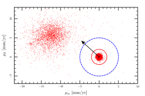
Figure 1.— Proper motions of the objects identified as stars in the ACS field. Since we used cluster members to define the reference frame, the zero point of the vector-point diagram corresponds to the bulk motion of the cluster. Those stars within the inner red circle comprise the sample to determine the color-magnitude diagram of the cluster. The stars within the outer blue dashed circle comprise the sample used to probe the proper-motion distribution. The arrow indicates a proper motion in the direction of the cluster center from the center of the ACS field. The swarm of stars centered around $\mu_{\alpha}\approx-12$ are field stars.

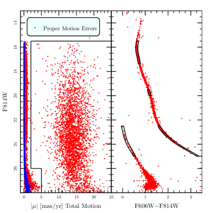
Figure 2.— Proper motions, proper-motion errors and colors as a function of magnitude. The left panel give the observed total proper motions as a function of apparent magnitude in red, and the proper motion errors in blue. The right panel plots the apparent magnitude against the observed color. Furthermore, the boxes depict the four subsamples outlined in §3.1.

3. Methods

3.1. Star Selection

To construct a member-only color-magnitude diagram, we select only those stars with proper motions (Fig. 1 and 2) relative to the mean motion of the cluster stars of less than 2 mas/yr for $15.5<\mathrm{F814W}<26$ (red circle) and proper-motion errors (blue points in Fig. 2 and all subsequent figures) of less 0.4 mas/yr. All stars brighter than $\mathrm{F814W}=15.5$ are used to construct the color-magnitude diagram, but because proper motions were not determined for these stars, they do not end up in the proper-motion sample. For stars fainter than $\mathrm{F814W}=26$, the proper-motion cutoff is 5 mas/yr and there is no error cutoff. field stars outside of the cluster comprise the broader distribution centered around $|\mu|\approx 15$ mas/yr on the left panel of Fig. 2.

Selecting the stars moving with the cluster yields the color-magnitude diagram (right panel of Fig. 2) from which the proper-motion sample is constructed. To prevent biasing the selected proper-motion sample, the cutoff in proper motion for this sample is 5 mas/yr and a proper-motion error cutoff of 0.4 mas/yr for all magnitudes. The sample is further winnowed by including only stars with colors that are within 0.05 magnitudes of the main-sequence and the white-dwarf cooling track. Table 3 gives some statistical properties of the objects that we identify as cluster and field stars. We focus on two large subsamples to probe the mass segregation of the cluster in radius. In particular, sample R1 consists of main-sequence stars with $17<\mathrm{F814W}<19.5$ that have a typical mass of about $0.5\mathrm{M}_{\odot}$. The second sample R2 probes fainter MS stars ($21<\mathrm{F814W}<22.5$) with a typical mass of $0.2\mathrm{M}_{\odot}$. Here we want to maximize the size of the samples to be sensitive even to subtle differences in the radial distributions without allowing the two samples to overlap. The samples R1 and R2 represent a compromise.

We also need to select some samples to investigate the dynamics of the cluster through the proper motions. Our results concerning the proper motions of the population as a whole focus on those stars with the most precisely measured proper motions, the “Best PMs” sample, the main-sequence stars with $19.5<\mathrm{F814W}<24.5$ — all of these PMs were measured using the long exposures, making a uniform sample. To probe the dynamical relaxation of the cluster we will define four smaller samples. Two of these are subsamples of the “Best PMs” sample, and two come from other regions of the color-magnitude diagram:

1. White dwarfs with $22.5<\mathrm{F814W}<25$ (“Bright White Dwarfs”),

2. Main-sequence stars with $22.5<\mathrm{F814W}<25$ (“Faint MS”),

3. Main-sequence stars with $19.5<\mathrm{F814W}<20$ (“Middle MS”),

4. Main-sequence stars with $15.5<\mathrm{F814W}<17.38$ (“Bright MS”).

Sample 1 contains 46 white dwarfs with the best measured proper motions. Sample 2 contains 254 main-sequence stars with well-measured proper motions over the same range of apparent magnitude as the white dwarfs. The size of sample 2 sets the goal size for the remaining subsamples. Sample 3 consists of 255 main-sequence stars, the brightest stars with proper motions measured from the long exposures. Furthermore, these main-sequence stars are expected to have a mass similar to the white dwarfs. Finally, sample 4 consists of the brightest 255 main-sequence stars with proper motions (here measured in the short exposures). This final sample provides our best estimate of the dynamical properties of the progenitors of the white dwarfs. The three main-sequence samples have the nearly the same size, allowing a fair comparision each sample with the white-dwarf sample. All four subsamples are depicted in the color-magnitude diagram. Table 3 gives the astrometric errors of the entire sample as well as the smaller subsamples.

Table 3Proper-motion dispersions, root-mean-squared errors, mean errors for the various subsamples

		Median		$\sigma_{\mu}$	${\hat{\sigma}}(\mu)$	Mean Error	RMS Error	$f$
Sample	Number	F814W	Mass	[mas yr-1]	[mas yr-1]	[mas yr-1]	[mas yr-1]	[%]
All stars	6345	21.6	—	5.42	1.31	0.07	0.10	0.30
All MS stars	2880	20.3	0.34	0.36	0.37	0.03	0.04	0.58
All WD stars	186	26.1	0.53	0.50	0.47	0.23	0.25	15.67
All field stars	3279	23.3	—	4.40	2.79	0.09	0.12	0.10
Radal Samples:
R1 (MS: $17<\mathrm{F814W}<19.5$)	788	18.3	0.58	0.37	0.37	0.05	0.05	1.09
R2 (MS: $21<\mathrm{F814W}<22.5$)	736	21.6	0.18	0.38	0.37	0.03	0.03	0.28
Proper-Motion Samples:
Best PMs (MS: $19.5-24.5$)	1899	21.0	0.24	0.37	0.37	0.03	0.03	0.30
Bright WD stars (1, $22.5-25$)	46	24.3	0.53	0.34	0.32	0.08	0.09	4.15
Faint MS stars (2, $22.5-25$)	254	23.1	0.11	0.37	0.38	0.05	0.05	0.83
Middle MS stars (3, $19.5-20$)	255	19.8	0.42	0.34	0.35	0.02	0.02	0.23
Bright MS stars (4, $15.5-17.38$)	255	16.7	0.74	0.34	0.34	0.04	0.05	1.04

The quantity $f=1-{\hat{\sigma}}_{n,\mathrm{true}}/{\hat{\sigma}}_{n,\mathrm{obs}}$ gives the relative decrease in the value of the velocity dispersion after correcting for the uncertainty in the observed proper motions. The “All Stars” sample has no proper-motion cutoff; whereas the non-fieldx other samples have a proper-motion cutoff of 5 mas/yr. All samples have an proper-motion-error cutoff of 0.4 mas/yr. The masses of main-sequence stars are given in solar masses using the models of Hurley et al. (2008) and assuming a distance of 2.53 kpc. The masses for the white dwarfs come from the spectroscopic measurements of Kalirai et al. (2008).

3.2. The ACS Field

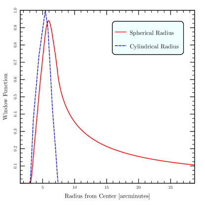
Figure 3.— The projected (blue dashed) and spherical radii (red solid) probed by the ACS field.

To efficiently average over the ACS field (depicted in Fig 20 with the potential stellar escapers), we define a window function that quantifies the regions of the cluster probed by the field. In the plane of the sky, the window function is simply defined to be proportional to the ratio of the area of the ACS field at a given projected radius from the center to the total area at that radius. The geometry of the field provides the initial guess of the window function. The estimate of the window function is optimized using the assumption that those stars in the field that are not cluster members are uniformly distributed.

For convenience the window function is normalized to unity at its peak. The three-dimensional window function is defined similarly: the ratio of the total volume within the field as extended through the cluster at a given three-dimensional radius from the center to the total volume at that particular radius. Again this function is normalized to unity at its peak. These window functions, as depicted in Fig. 3, provide a useful technique to generate either a Monte Carlo sample or integrate over the three-dimensional structure of the cluster. The window function is simply the probability that a particular star in the entire Monte Carlo sample ends up in the sample that represents the field.

3.3. Theoretical Model

To obtain estimates of the total mass of the cluster and the escape velocities of individual stars, we will rely on a theoretical model of the cluster. We will use the model as one method of deprojecting our velocity and surface density measurements to constrain the dynamical properties of the cluster. This section outlines the model and the statistical measures that we will used to characterize both the model and the data. An appendix derives several useful results from the model that further our interpretation of the data.

To model the stars in the globular cluster we will assume that the phase-space density is given by a lowered Maxwellian distribution (Michie, 1963; King, 1966),

$$f(E)=N\left[\exp(-E/\sigma^{2})-1\right]$$ (1)

where $N$ is the normalization, $E$ is the energy of a star per unit mass (less than zero because the stars are bound) and $\sigma$ is a parameter with dimensions of velocity that sets the velocity scale for a particular group of stars in the cluster. Let $\Psi(r)$ be the negative of the potential energy, which vanishes at the edge of the cluster (the tidal radius, $r_{t}$) so the number density of stars at a radius $r$ is

$$n(r)=\frac{\rho_{1}}{\left(2\pi\sigma^{2}\right)^{3/2}}\int_{0}^{v_{e}}4\pi v^{2}\left[e^{(v_{e}^{2}-v^{2})/(2\sigma^{2})}-1\right]dv$$ (2)

where $\rho_{1}$ is the number density normalization, $v$ is the speed of the star and $v_{e}^{2}=2\Psi(r)$ is the speed needed to escape the cluster by reaching the tidal radius. Therefore, the number density is given by

$$n(r)=\rho_{1}\left[e^{v_{e}^{2}/(2\sigma^{2})}\mathrm{erf}\left(\frac{v_{e}}{\sqrt{2}\sigma}\right)-\sqrt{\frac{2}{\pi}}\frac{v_{e}}{\sigma}\left(1+\frac{1}{3}\frac{v_{e}^{2}}{\sigma^{2}}\right)\right].$$ (3)

Similarly the local three-dimensional velocity dispersion is given by

$$\overline{v^{2}}(r)=\frac{J_{2}}{J_{0}}$$ (4)

where

$$J_{n}=\int_{0}^{v_{e}}\left[e^{(v_{e}^{2}-v^{2})/(2\sigma^{2})}-1\right]v^{n+2}dv.$$ (5)

To build a model star cluster we take a range of stellar masses each with in its own value of $\sigma$ in Eq. 3; the stars of different masses are assumed to be in thermal equilibrium, i.e. $m_{i}\sigma_{i}^{2}$ is a constant. This provides the total mass density of stars as a function of the local potential. We select a value for the central potential and integrate the Poisson equation for the gravitational potential using the total mass density of the ensemble of stars as a source. For each value of the central potential, we vary the normalizations of the mass densities ($\rho_{1})$ for each mass to match the observed mass function of NGC 6397 (Richer et al., 2008). This generates the value of the potential as a function of radius, yielding the number density, column density and the one-dimensional velocity dispersion as a function of radius for any subpopulation of stars with a particular value of $\sigma$. We then choose the values of the central potential and $\sigma$ that yield the best match to the photometry of NGC 6397(Trager et al., 1995). §4.1 compares the observational results from this work and previous work with the theoretical model of the cluster outlined here, and the appendix derives several properties of this model that are useful to interpret the observational results.

We would like to compare these model distributions against the data and characterize these distributions using standard deviation of the velocity distribution along a particular direction. The standard deviation has several advantages including the ease of calculation from both the models and the data and a straightforward physical interpretation, in the Jeans equation, for example. However, the standard deviation is extremely sensitive to outliers. In fact a single interloping star, say from the Galaxy, in the sample could ruin our estimate of the standard deviation of the stars within the cluster. There are several robust estimators of the scale or width of a distribution, such as the median absolute deviation or for two-dimensional distributions like the proper motion, the median magnitude of the proper motion. These two estimators are maximally insensitive to outliers; up to half of the points can be shifted to arbitrarily large values without affecting the result. For a normal distribution these estimators yield values proportional to the standard deviation; however, as the distributions deviate from normality such as those present in the lowered isothermal sphere, these constants of proportionality can change.

Instead of these estimators we use the first quartile of the differences of the proper motions along a particular direction to estimate the standard deviation of the distribution: (the estimator $Q_{n}$ defined by Rousseeuw & Croux, 1993)

$${\hat{\sigma}}=d_{n}\times\text{firstquartileof}\left(\left|\mu_{i}-\mu_{j}\right|:i<j\right).$$ (6)

where $\mu_{i}$ and $\mu_{j}$ are the measured proper motions of stars in our sample or the model along a particular direction and $d_{n}$ is a factor that depends on the size of the sample that ensures the ${\hat{\sigma}}$ is an unbiased estimator of the standard deviation for normally distributed data. As the sample size diverges ($n\rightarrow\infty$), $d_{n}$ approaches $1/(2\mathrm{erf}^{-1}(1/4))\approx 2.219$. Like the medians discussed earlier, the estimator ${\hat{\sigma}}$ has a breakdown point of 50%, meaning that one could shift up to one half of the values $\mu_{i}$ to infinity without affecting the estimator.

The estimator $\hat{\sigma}$ has several further advantages. First, it can be determined for each direction, unlike the median magnitude of the proper motion. Second, the value of $\hat{\sigma}$ approximates well the standard deviation for distributions that differ significantly from Gaussian such as a uniform distribution. Finally, the estimator $\hat{\sigma}$ is statistically efficient, meaning for a sample of a given size the typical error is smaller than that which results for the median absolute deviation or median proper-motion magnitude.

We calculate ${\hat{\sigma}}$ from the proper-motion data, the radial velocity sample and from the models. Additionally we treat ${\hat{\sigma}}$ as a proxy for the standard deviation for much of our analysis. In particular, when we correct our observed proper motions for the estimated errors in the proper motions, we will use

$${\hat{\sigma}}^{2}_{\mu,\mathrm{true}}={\hat{\sigma}}^{2}_{\mu,\mathrm{obs}}-\frac{1}{n}\sum_{i=1}^{n}\epsilon_{i}^{2}$$ (7)

where $\epsilon_{i}$ is the proper-motion error of each star. Table 3 shows that these corrections are generally small. Finally as we shall see in § 4.7 the Jeans equation uses the velocity variance to provide an estimate of the mass of the cluster; therefore, we shall use both observed proper-motion variances and $\hat{\sigma}$ to estimate the mass of NGC 6397. We shall find that the values of $\hat{\sigma}$ and the standard deviation are approximately equal for most of the subsamples that we investigate, so this choice makes little difference to the final mass estimates.

3.4. Error Estimation

The statistical bootstrap, the cousin of the Quenouille-Tukey jackknife, was introduced by Efron in 1977 (Efron, 1979). In this section we introduce or rather reintroduce the bootstrap and outline how we use it to estimate the errors in our derived proper-motion dispersions, column density distributions and cluster mass. (Refer to Lupton 1993 for further details). Observations of NGC 6397 draw a sample of $n$ stars with positions and velocities $\{(\vec{x}_{i},\vec{v}_{i})\}_{0}$ from the phase–space distribution function, $f(\vec{x},\vec{v},t_{0})$. We use various statistics of the observed stars to make conclusions about the distribution function and its evolution: for example, the mean position along the $\alpha$-axis of the sample:

$$\bar{x}_{\alpha}={1\over n}\sum_{i}x_{\alpha,i}$$ (8)

and its associated error

$$\sigma^{2}_{\bar{x}_{\alpha}}={1\over n}{1\over n-1}\sum_{i}(\bar{x}_{\alpha}-x_{\alpha,i})^{2}.$$ (9)

By performing these summations, we assumed that the statistics of the set $\{(\vec{x}_{i},\vec{v}_{i})\}$ are a good approximation to those of the actual phase–space distribution function, $f(\vec{x},\vec{v},t_{0})$. This is also the assumption behind statistical bootstrapping.

However, we could have taken a more complicated route and created another distribution function (in fact the distribution that maximizes the likelihood of the observations),

$$f^{*}={1\over N}\sum_{i}\delta(\vec{x}-\vec{x}_{i},\vec{v}-\vec{v}_{i}),$$ (10)

and then calculated mean position by taking the integral over the region probed by the ACS observations,

$$\bar{x}_{\alpha}=\int_{\mathrm{ACS~{}Field}}x_{\alpha}f^{*}d\vec{x}d\vec{v}.$$ (11)

Now we have two methods to estimate the error in our determination of the center of mass: calculating an integral analogous to the second summation (Equation 9), or drawing a variety of samples from our new distribution function $f^{*}$ and investigating the distribution of $\bar{x}_{\alpha}^{*}$. Our original sample, $\{(\vec{x}_{i},\vec{v}_{i})\}$, is now only one of many possible realizations of $f^{*}$, and the distribution of $\bar{x}_{\alpha}^{*}$ over the various resamplings approximates the distribution of $\bar{x}_{\alpha}^{*}$ over $f^{*}$ (Lupton, 1993) which we in turn assume to approximate $f(\vec{x},\vec{v},t_{f})$. Thus, through resampling we can estimate the error in our determination of $\bar{x}_{\alpha}^{*}$ given by Equation 9. This Monte–Carlo resampling is less expedient than using Equation 9, but often we do not have the luxury of a statistic defined as simply as $\bar{x}_{\alpha}$ is in Equation 8. Even more rarely do we have the luxury of a straightforward analytic error estimator like Equation 9.

So how is the bootstrap implemented with ACS observations? Ordinarily when one calculates a physical value from a sample, one uses all the stars, counting each one once. To use the bootstrap, one simply needs to select from an $n$–star sample, $n$ stars with replacement. To create a bootstrapped sample, we uniquely label each of the stars in an $n$-star sample from 1 to $n$. We then select $n$ integers from 1 through $n$ and use the stars with the appropriate labels to create a new ensemble. Some of the stars in the original sample are included in the new ensemble several times and others not at all. We often use the value of ${\hat{\sigma}}$ for a sample of proper motions to characterize them. We resample each group of stars 1,000 times, determine the value of ${\hat{\sigma}}$ of each resampling, sort the results and quote the fifth and ninety-fifth percentiles as a ninety percent confidence region. In § 4.7 we estimate the mass of NGC 6397. In this case we calculate a mass estimate for each resampling, sort these results and calculate the ninety-percent confidence region for the final result.

4. Results

This section begins with a theoretical model for the cluster (§ 4.1) to provide a context for various characteristics of the data including the radial distribution (§ 4.2), proper motions (§§ 4.3-4.5) and some derived properties of these data including its distance (§ 4.6) and mass (§ 4.7).

4.1. A Model for NGC 6397

The mass function of Richer et al. (2008) and the observed concentration of the cluster from Trager et al. (1995) provide a useful starting point to construct a preliminary multi-mass King model for the cluster from which we can draw some global inferences. Fig. 4 compares the model surface density for the best fitting values of the central escape velocity and dispersion parameter ($\sigma$) with the observed photometry from Trager et al. (1995). We have also included the star counts within our field; § 4.4 and Fig. 13 presents these counts in further detail. To convert the star counts to an estimate of the surface brightness we convert the ACS magnitudes used here to the Johnson system using the synthetic transformations of Sirianni et al. (2005). This yields the total flux from all of the stars in the CMD sample defined in Fig. 2 of $V_{\mathrm{total}}=9.75$ within the ACS field of 10.9 square arcminutes. This gives a mean surface brightness of 21.23 $V$ magnitudes per square arcsecond or equivalently a mean $V-$magnitude of 17.94 for each main-sequence star in the proper-motion sample used to calculate the results depicted in Fig. 13. The star counts as a function of projected radius are scaled by this mean magnitude per star, yielding the blue squares in Fig. 4.

The radial, magnitude, velocity normalizations, central velocity dispersion and $\sigma-$parameter of the models are arbitrary, and a comparison with the data is used to set the scale of the model. We use the models of Hurley et al. (2008) to set the ratio of the $\sigma-$parameter of the turn-off stars, which are assumed to provide the bulk of the light, and that of the proper-motion sample. We take the mass of the turn-off stars to be $0.84~{}\mathrm{M}_{\odot}$ and the proper-motion sample to be $0.24~{}\mathrm{M}_{\odot}$. Furthermore, we assume that the values of $\sigma$ following the equiparition relation with same value $m_{i}\sigma_{i}^{2}$ to the various populations. The values of $\sigma$ and $\mu_{e,0}$ are determined with an unweighted least-squares fit between the models and the data. The bulk of the points in this fit are provided by the Trager et al. (1995) photometry; however, a measurement of the velocity dispersion is required to set the velocity scale of the models. Here, we also use the data from § 4.4 and Fig. 13. Fig. 5 depicts the observed proper motions, those found in the model and the observed radial velocities of MM91 for different assumed distances.

Both the gross properties of the cluster such as its mass and the profile near the half-light radius depend little on the properties of the central regions. Operationally the radial scale and the ratio of the central escape velocity to the $\sigma$-parameter are determined mainly by the surface photometry (Fig. 4) and the velocity normalization is determined by the value of ${\hat{\sigma}}$ as a function of radius (Fig. 5). The two crucial parameters for the model are the central escape proper motion of $\mu_{e,0}=2.31$ mas/yr and the $\sigma$-parameter of 0.54 mas/yr for the turn-off stars that dominate the light and 1.01 mas/yr for the stars in the proper-motion sample. For the brightest stars, the value of the $\sigma$-parameter is approximately the central velocity dispersion along one dimension because $\mu_{e,0}\gg\sigma$. The ratio of these two quantities is determined mainly by the surface brightness profile while the normalization is determined exclusively by the proper-motion data depicted in Fig. 5.

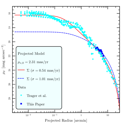
Figure 4.— Surface photometry as measured by Trager et al. (1995) (cyan crosses) and surface star counts from this work (blue squares) compared the the model surface density for the best fitting stars in the model (red solid curve) and the most massive stars in the model (blue dashed curve).

The observed velocity dispersion, either in the radial direction or in a particular direction of proper motion, is integrated over the line-of-sight so we can project the model onto the plane of the sky. Figure 5 depicts both of these results. Beyond one half-light radius the observed velocity dispersion depends only very weakly on the $\sigma$-parameter, so although mass segregation is important in generating the radial distribution, the velocity dispersions are nearly independent of stellar mass. Furthermore, the escape velocity at a given radial distance from the center of the cluster is typically three times the velocity dispersion within five-percent agreement with the analytic treatment in the appendix (Eq. A7).

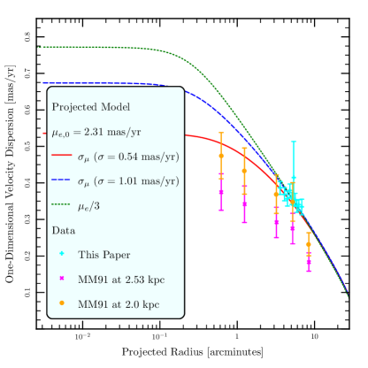
Figure 5.— Projected velocity dispersion as a function of projected radius: model (best-fitting stars in red and most massive stars in green), radial-velocity and proper-motion measurements. The velocity measured of Meylan & Mayor (1991) (MM91) have been converted to proper motions assuming a distance of 2.55 kpc (Richer et al., 2008) and 2 kpc to bring agreement between the proper-motion and radial-velocity measurements. The error bars from this paper are ninety-percent confidence intervals obtained by bootstrapping. The errorbars on the MM91 data are 1.64-$\sigma$.

Fig. 4 shows that the change in the slope of the surface brightness profile as a function of the $\sigma$-parameter (or mass) is largest around one arcminute from the center of the cluster. The difference in slopes is more modest at the projected radius of the ACS field; therefore, the mass segregation in the model is weaker here. The analytic treatment outlined in the appendix although illustrative, is not strictly applicable here, because the escape proper motion is approximately 1 mas/yr and the $\sigma$-parameter is 1.01 mas/yr, so the value of $\sigma$ approximates that of $\mu_{e}$ and does not greatly exceed it. The field is not in the regime where the distribution function is strictly linear, however, as we can see from Fig. 5.

The model velocity and distance normalizations also yield a model mass for the cluster of

$$M=1.1\times 10^{5}d_{2.53}^{3}\mathrm{M}_{\odot}$$ (12)

where $d_{2.53}$ is the distance to NGC 6397 from Earth divided by 2.53 kpc. We can combine the mass estimate in Eq. 12 with the mean stellar mass of about $m_{*}=0.35~{}\mathrm{M}_{\odot}$ (Dotter et al., 2007; Richer et al., 2008) to obtain an estimate of the relaxation time at the half-mass radius (Spitzer & Hart, 1971)

$$\tau_{rh}=0.138\frac{M^{1/2}R_{h}^{3/2}}{m_{*}G^{1/2}\ln\left(0.4M/m_{*}\right)}$$ (13)

to yield $\tau_{rh}=0.45d_{2.53}^{3}$ Gyr where we have suppressed the additional logarithmic dependence on distance through the Coulomb logarithm.

4.2. Mass Segregation

Fig. 6 depicts the cumulative radial distribution of several groups of stars in the sample, including two of the subsamples described in § 3.1 and Table 3. If we compare the main sequence stars with $17<\mathrm{F814W}<19.5$ and $21<\mathrm{F814W}<22.5$, we obtain a $p-$value of $7\times 10^{-5}$ by the Wilcoxon rank-sum test and twice this value for the Kolmogorov-Smirnov (KS) test, indicating that it is highly unlikely that these two groups of stars follow the same radial distribution. The two main sequence samples show significant segregation, even greater than the model distributions. The model distributions are typically more centrally concentrated than the stars in the ACS field because they are based on the surface photometry as outlined in § 4.1. Because the field lies outside the half-light radius, following the arguments of § 3.3, we do not expect mass segregation to be strong in this region and the model exhibits only weak mass segregation. Either the cluster has stronger mass segregation than the model, or perhaps the samples are incomplete especially for fainter stars near the center. Because the incompleteness fraction is low (less than 7% for the stars in these two samples), we can discount the second possibility. Although we will present the observed column density of stars within the field and use this to estimate the radial density gradient, we use this gradient as input for only two of several independent mass determinations in § 4.7, the results of which agree with the mass determination from surface brightness measurements.

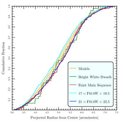
Figure 6.— Cumulative projected radial distribution for various subsamples. The three model curves give the best-fitting model in the middle (a mass of 0.35 M_⊙ or F814W $\sim 21$) and models for two other masses assuming that $m_{i}\sigma_{i}^{2}$ is constant. The models of Dotter et al. (2007) give the correspondence between masses and magnitudes. The left-hand model traces the distribution for a stellar mass of 0.58 M_⊙ (F814W $\sim 18$), and the right hand for a mass of 0.18 M_⊙ (F814W $\sim 22$).

Fig. 6 serves a second purpose. Although the faint MS and bright WD samples span the same magnitude range, the stars in the WD sample are typically fainter than in the MS sample as shown in Table 3. In § 4.5 we shall argue that these two samples have significantly different proper-motion distributions; in principle, this could result from the two samples having different radial distributions. The typically fainter white dwarfs might be more difficult to find toward the center of the cluster, biasing this sample outward and biasing the proper-motion distribution toward smaller values. The cumulative distributions depicted in Fig. 6 demonstrate that this is unlikely. A comparison of the radial distribution of the two samples yields a $p-$value of 89% by the KS test and 92% by the Wilcoxon rank-sum test.

We also compare the radial distribution of the 46 bright white dwarfs with the two larger main sequence samples and find probabilities of 98% and 48% from the KS tests, and 92% and 32% Wilcoxon rank-sum probabilities. Furthermore, when we compare the radial distribution of bright white dwarfs ($22.5<\mathrm{F814W}<25$) with a sample of 97 fainter white dwarfs ($25<\mathrm{F814W}<26.5$ – not shown in Fig. 6), we find 54% KS and 51% Wilcoxon probabililties. This fails to support the conclusions of Davis et al. (2008b) which used a smaller sample to conclude that the distribution of young white dwarfs was radially extended relative to that of older ones and argue that a possible explanation for this phenomenon was a white-dwarf natal kick.

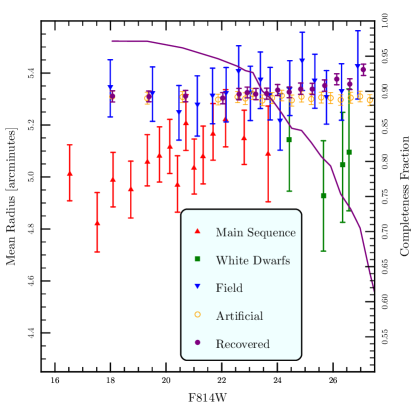
Figure 7.— Mean projected radius of stars as a function of F814W. The open circles give the mean radius for the input artificial stars, and the closed circles give the mean radius of those recovered. The errorbars here and in subsequent figures represent ninety-percent confidence limits and are obtained by bootstrapping. The solid curve gives the completeness fraction as a function of apparent magnitude as calculated from the artificial star tests. This curve is read using the right-hand axis.

A possible explanation for the differing distributions as a function of apparent magnitude is differential incompleteness. It is more difficult to find faint stars in more crowded areas of the sky near the centre of the cluster. We have addressed this question in several ways in Fig. 7. First we have looked at the stars in the image and sorted them by apparent magnitude into bins of 50 white-dwarf stars or 200 main-sequence or field stars. A priori we do not expect the field stars (at any magnitude) to be centrally concentrated with respect to the cluster, so a change in the mean radius of the field stars would have to result from differential incompleteness. Because the number of field stars is limited to about 3,000, to get a better statistical handle on this effect, we inserted nearly 200,000 artificial stars throughout the image of various magnitudes and tried to recover them. The recovery fraction depicted by the solid curve in Fig. 7 gives an estimate of the completeness fraction. The mean radius of the input stars as a function of magnitude is given by the open circles. The mean radius of the recovered stars is given by the closed circles. We have sorted the artificial stars into bins of 5,000 objects. We see that fainter than $\mathrm{F814W}\approx 23$ the recovered stars are on average further from the cluster centre than the input stars, the hallmark of differential incompleteness by about 0.05 arcminutes; however, the effect is much more subtle than the change in the mean radius along the main sequence and white-dwarf tracks. It is unlikely to be strong enough to account to the differences in the radial distirbutions depicted in Fig. 6 where the median radius of the models differs from the data by more than a tenth of an arcminute..

4.3. Proper-Motion Isotropy

We measure the angle of the proper motion relative to the cluster center of the main-sequence stars with $19.5<\mathrm{F814W}<24.5$, proper-motion errors less than 0.4 mas/yr and total proper motions less than 5 mas/yr. The distribution of this angle is depicted in Fig. 8. There is no evidence for anisotropy from this distribution — a KS test indicates that the cumulative distribution of 35% of samples drawn from a uniform distribution will differ from uniform at least as much as the distribution in Fig. 8 does. The $p-$value for the Kuiper test (1960, a generalization of the KS test for a distribution on a circle) is smaller at 13%. If we look at the direction of the proper motions relative to right ascension and declination, the $p-$value for the KS test increases to 39% and for the Kuiper test to 32%. The directions alone do not reveal any anisotropy.

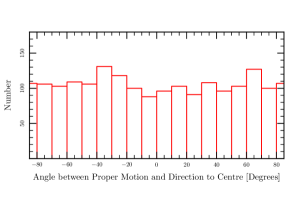
Figure 8.— Histogram of proper-motion angle relative to the center of NGC 6397.

We can also compare the velocity dispersion along the radial direction ($\hat{\sigma}_{R}$) to the tangential direction ($\hat{\sigma}_{T}$) for the main-sequence stars with the most precisely measured proper motions ($19.5<\mathrm{F814W}<24.5$) and find that ${\hat{\sigma}}(\text{radial})/{\hat{\sigma}}(\text{tangential})=0.96\pm 0.04$, i.e. just consistent with isotropy at 90% confidence. To examine this in greater detail we sort the main-sequence stars and white-dwarf stars by apparent magnitude into subsamples of 200 stars for the main sequence and 50 stars for the white dwarfs (the faintest subsample may contain fewer). The proper motions are measured in the radial and tangential directions (relative to the center of the cluster) and the ratio of the dispersion in the radial direction to that in the tangential direction is determined and depicted in Fig. 9. We can divide the sample by the projected radius (Fig. 10) or total proper motion (Fig. 11). As for the distribution of all the proper motions for stars with $19.5<\mathrm{F814W}<24.5$, we see no strong evidence for anisotropy in any of these subsamples. We also relaxed the assumption that the proper-motion ellipse is aligned with the radial or tangential direction and even in this more general case found no evidence for anisotropy in either the entire sample or the subsamples. The aforementioned results describe the proper-motion ellipse relative to the center of the cluster. We can also examine the proper-motion ellipse relative to the field boundaries. For the total proper-motion sample and the various subsamples, we do not find any evidence for anisotropy of the proper motions relative to the boundary of the field.

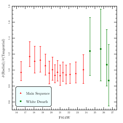
Figure 9.— The radial anisotropy of the proper-motion ellipse as a function of apparent magnitude for main-sequence and white-dwarf stars. Only stars with total proper-motion error less than 0.4 mas/yr are included.

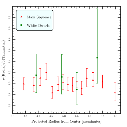
Figure 10.— The radial anisotropy of the proper-motion ellipse as a function of projected radius from the center for main-sequence and white-dwarf stars. Only stars with total proper-motion error less than 0.4 mas/yr are included.

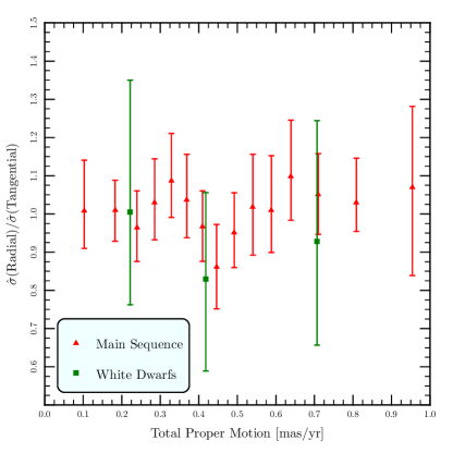
Figure 11.— The radial anisotropy of the proper-motion ellipse as a function of total proper motion for main-sequence and white-dwarf stars. Only stars with total proper-motion error less than 0.4 mas/yr are included.

4.4. Proper-Motion Dispersion

To examine the proper-motion dispersion, we sort the main-sequence and white-dwarf samples by apparent magnitude into subsamples of 200 and 50 stars, as before. We calculate the value of ${\hat{\sigma}}$ for each subsample in the radial (${\hat{\sigma}}_{R}$) and tangential directions (${\hat{\sigma}}_{T}$) and define the one-dimensional value of

$${\hat{\sigma}}=\frac{\sqrt{{\hat{\sigma}}_{R}^{2}+{\hat{\sigma}}_{T}^{2}}}{2}.$$ (14)

Because the proper motions are nearly isotropic, the value in either direction is well approximated by the one dimensional value of ${\hat{\sigma}}$ as defined above. Furthermore, for a spherically symmetric stellar system even if the velocity distribution is not isotropic, by extending the results of Leonard & Merritt (1989) we find that

$$\sigma_{R}^{2}+\sigma_{T}^{2}=2\sigma_{z}^{2}$$ (15)

where $\sigma_{z}$ is the velocity dispersion along the line of sight; therefore, Eq. 14 gives the natural value to compare with radial-velocity measurements, such as MM91. The root-mean-squared error in the proper motion is scaled and subtracted from each estimate of the dispersion (and its confidence interval) in quadrature (see § 3.3 for more details).

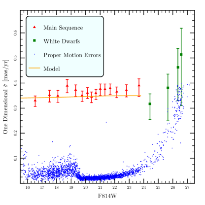
Figure 12.— The value of ${\hat{\sigma}}$ as a function of apparent magnitude.

Fig. 12 shows that the proper-motion dispersion is nearly constant, possibly increasing slowly with fainter magnitudes at the bright end and nearly constant for $\mathrm{F814W}>19$ along the main sequence. Such a weak trend is expected for a sample beyond the half-light radius of the cluster because the velocity distribution is cut off by escaping stars as shown by the model curve. The trend in the data is a bit stronger than the model. The observed proper motions of the brightest fifty white dwarfs are smaller by nearly two standard errors than those of the faintest eighty main-sequence stars — $\hat{\sigma}_{WD}-\hat{\sigma}_{MS}=-67~{}\mu\mathrm{as/yr}$ with a standard error of $36~{}\mu\mathrm{as/yr}$. The distribution of the differences in the dispersion over the bootstrapped resamplings is approximately normal and the probablility that $\hat{\sigma}_{WD}>\hat{\sigma}_{MS}$ is about three percent. The main-sequence stars with masses similar to the white dwarfs have $\mathrm{F814W}\approx 18.8$. If we take the two hundred main-sequence stars with a median magnitude of 18.8 and calculate $\hat{\sigma}_{WD}-\hat{\sigma}_{MS}$, we obtain $-90~{}\mu\mathrm{as/yr}$ with a one-percent chance that $\hat{\sigma}_{WD}>\hat{\sigma}_{MS}$. If we take the brightest two hundred main-sequence stars, we obtain a closer agreement with $\hat{\sigma}_{WD}-\hat{\sigma}_{MS}=-26~{}\mu\mathrm{as/yr}$ and a 17% chance that $\hat{\sigma}_{WD}>\hat{\sigma}_{MS}$. If we take the brightest fifty main-sequence stars, the difference decreases to $-14~{}\mu\mathrm{as/yr}$, and the probability increases to 38%. Looking along the main sequence to brighter magnitudes, it is apparent that the best agreement is with the brightest stars in the proper-motion sample; these stars most resemble the progenitors of the white dwarfs.

With a sample of about 2000 main-sequence stars with $19.5<\mathrm{F814W}<24.5$, we sort the stars in projected radial distance from the center of the cluster and determine the dispersion as a function of radius as shown in Fig. 13. In this case each subsample consists of 200 stars. Again the confidence intervals are determined by resampling, and the root-mean-square error in proper motion is subtracted from ${\hat{\sigma}}$ as described in § 3.3. Both the density and proper-motion dispersion decrease with increasing radius. The curves give the best-fit power-law functions of radius for the value of ${\hat{\sigma}}$ and column density. We have

$${\hat{\sigma}} \approx \left(0.37\pm 0.06\right)\left(\frac{R}{5^{\prime}}\right)^{\!\!-0.21\pm 0.09}\!\!\!\!\!\mathrm{mas~{}yr,}^{\!-1}$$

$$\Sigma \approx \left(0.048\pm 0.030\right)\left(\frac{R}{5^{\prime}}\right)^{\!\!-1.40\pm 0.38}\!\!\!\!\!\frac{\mathrm{stars}}{\mathrm{arcsecond}^{2}}.$$ (16)

We can also use the proper motions and positions themselves without binning in radius to determine the best fitting power-law relations for the column density and velocity dispersion, yielding

$$\sigma_{\mu} \approx 0.36\left(\frac{R}{5^{\prime}}\right)^{\!\!-0.18}\!\!\!\!\!\mathrm{mas~{}yr,}^{\!-1}$$

$$\Sigma \approx 0.053\left(\frac{R}{5^{\prime}}\right)^{\!\!-1.32}\!\!\!\!\!\mathrm{stars~{}arcsecond.}^{\!-2}$$ (17)

in good agreement with the fitted parameters for ${\hat{\sigma}}$ and the column density in Eq. (16) and the velocity dispersion fitted from Fig. 5 ($\sigma_{\mu}\approx 0.36(R/5^{\prime})^{-0.20}$)

For clarity we have not quoted errors on these parameters because they are intermediate results in the determination of the mass of NGC 6397, which appears in § 4.7 with error bars.

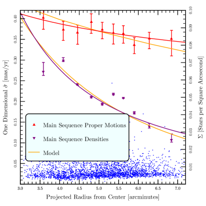
Figure 13.— The value of ${\hat{\sigma}}$ and stellar density as a function of projected radius. The red and purple curves trace the best-fitting power-law relations in radius to the data of the same color. The upper green curve traces the value of the proper-motion dispersion as a function of radius according to the model. The lower curve depicts the value of the projected stellar density according to the model.

Although the power-law fit to the value of ${\hat{\sigma}}$ characterizes the data well, the fit for the projected stellar density is poor. The observed star counts vary up and down with radius where any reasonable model would predict a monotonic decrease in radius. This behaviour appears to be larger than expected given the errors on the densities, so it probably reflects either inhomogeneities in the cluster or underestimated errors in our analysis. However, the models developed in § 4.1 rely only weakly on the projected stellar densities across the ACS field because they also account for the surface-brightness profile of the entire cluster from Trager et al. (1995).

The stellar density and velocity dispersion can provide an estimate of the relaxation time for a group of stars, (Spitzer & Hart, 1971)

$$\tau_{r}=\frac{0.065v_{\mathrm{RMS}}^{3}}{3G^{2}m_{*}^{2}n\ln(0.4M/m_{*})}$$ (18)

where $v_{\mathrm{RMS}}$ is root-mean-square velocity of the stars, $n$ is the number density, $M$ is the total mass of the cluster and $m_{*}$ is the mass of a typical star (taken to be 0.35 M_⊙). Using the results of Eq. 17 with our kinematic distance (Table 1 and § 4.6) yields

$$\tau_{r}\approx 0.6~{}d_{2}^{6}~{}\mathrm{Gyr}$$ (19)

at a radius of five arcminutes where $d_{2}$ is the distance to NGC 6397 divided by 2 kpc and we have deprojected the velocity and projected stellar densities using an inverse Abel transform (Leonard & Merritt, 1989). If we use the velocities measured by MM91 at five arcminutes (the approximate radius of our field) with the standard candle distance of 2.53 kpc (Gratton et al., 2003) yields the larger value of

$$\tau_{r}\approx 0.8~{}d_{2.53}^{3}~{}\mathrm{Gyr}.$$ (20)

We will revisit these timescales in the following section.

4.5. Proper-Motion Distribution

Our first focus will be the sample of about 2000 main-sequence stars with $19.5<\mathrm{F814W}<24.5$ as in the previous section. As MAM06 did, we look at the differential distribution of proper motions in various directions as well as the total proper motion. These directional distributions are presented in Fig. 14. Each of the distributions has been fit with a Gaussian (Maxwellian) distribution of proper motions in one dimension; the value of the standard deviation of the distribution is taken to be the value of $\hat{\sigma}$ for the sample of proper motions. One can conclude from an Anderson-Darling test (1952) that the proper motions in the radial and right ascension directions are not sampled from a Gaussian distribution at the 95% confidence level. The conclusion that the proper motions in the tangential and declination directions are not drawn from a Gaussian exceeds 99% confidence. The values of $\sigma$ for the various directions do not differ significantly from each other as one would expect from the results of § 4.3.

We can directly compare the various distributions with each other and look for significant differences using a KS test. Because the KS test is most sensitive to changes in the median values (here expected to be zero for all of the one-dimensional distribution), we compare the distribution of the absolute values of the proper motions. In particular the distribution of the proper motion toward or away from the cluster center (radial) or perpendicular to this direction (tangential) do not differ significantly as the KS test yields a $p-$value of 57%. On the other hand, the hypothesis that the proper motions in right ascension and declination are drawn from the same distribution can be rejected with nearly 99% confidence according to a KS test, indicating that there may be some residual systematics in the proper-motion measurements; however, the values of the dispersions of the best-fitting Gaussian agree well within the ninety percent confidence regions, so the differences are more subtle than the width of the distributions.

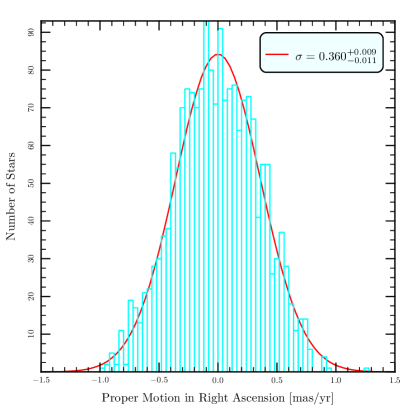
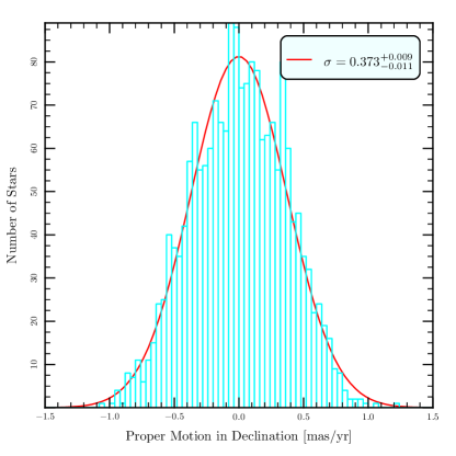
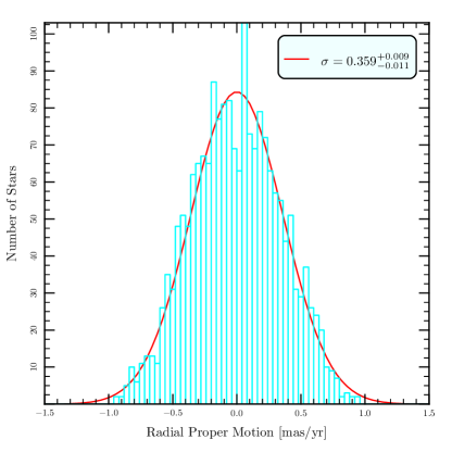
Figure 14.— Differential distributions of the observed proper motions in various directions and best-fitting Gaussians. The values of $\sigma$ are given in milliarcseconds per year.

The theoretical model that we developed in §§3.3 and 4.1 exhibits an isotropic velocity distribution, so it makes most sense to compare the model with the distribution of the total proper motion. We shall examine two theoretical models. First, the model yields an estimate of the proper-motion distribution over the entire field as depicted in Fig. 15. This proper-motion distribution results from convolving Eq. A9 in the appendix with the window function in spherical radius in Fig. 3. This proper model distribution yields a KS probability of two percent for the null hypothesis that the stars from the proper-motion sample are drawn from it. The results of Fig. 13 indicate a second possible treatment. The figure depicts the model results for the stellar column density and the dispersion (${\hat{\sigma}}$). Although the fit to the proper motion appears good, the model does not track the observed column density well. In fact the observed column density does not actually decrease monotonically with radius, indicating that possibly the cluster is a bit clumpy. However, we can also convolve the distribution in Eq. A10 with the number of stars as a function of radius in Fig. 13. This results in the “Scaled Model” in Fig. 15 that yields a KS probability of thirty-three percent for the null hypothesis that the observed proper motions of the nearly two thousand main-sequence stars in the proper-motion sample are drawn from the theoretical model.

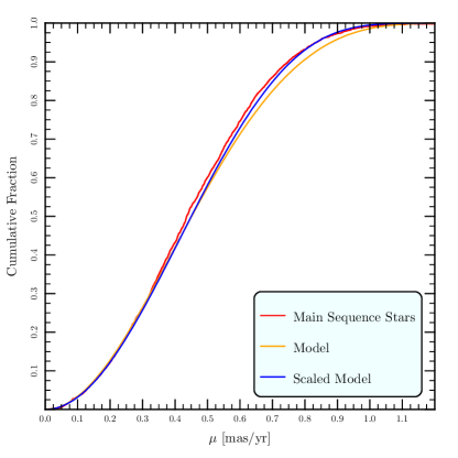
Figure 15.— Cumulative distribution of total proper motion for the main-sequence stars, the basic model and a model scaled to yield the observed column density in Fig. 13.

An examination of the differential distribution of the total proper motion yields additional details (Fig. 16). The width is similar to the one-dimensional results in Fig. 14. The distribution of stars cuts off much more quickly than the best-fitting Rayleigh distribution (the distribution of speeds if the velocity in each of two dimensions follows a Gaussian). The latter gives 49 stars with total proper motions exceeding one milliarcsecond per year; there were only six observed in the sample. If we assumed that the best fitting Rayleigh distribution was the underlying true distribution the chance of finding six when we expect 49 is about $10^{-14}$, assuming Poisson statistics. The cutoff at about one milliarcsecond per year results because the cluster has a finite escape proper motion at this radius of roughly one milliarcsecond per year. The results of § 4.1 produce a distribution of total proper motions using Eq. (A9) convolved with the window function shown as the “Model” curve in Fig. 16) or convolved with the observed number of stars as a function of radius from Fig. 13 shown as the “Scaled Model” curve.

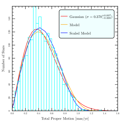
Figure 16.— Differential distributions of total proper motion for the main-sequence stars, the basic model and a model scaled to yield the observed column density in Fig. 13, and the best-fitting Gaussian. The value of $\sigma$ is given in milliarcseconds per year.

To contrast the distribution of white dwarfs and main sequence stars, we examine the subsamples delineated in Fig. 2 and Table 3. Fig. 17 depicts the cumulative proper-motion distributions for the four subsamples, and Table 4 gives the KS and Wilcoxon probabilities for each pair. Lower probabilities indicate that the null hypothesis that the two samples are drawn from the same underlying distribution is unlikely. The stars in the bright WD sample and faint MS sample span the same magnitude range, but a comparision of their proper-motion distributions yields $p-$value of 0.02 by the KS test. The main sequence stars with $\mathrm{F814W}\approx 19$ (middle MS) are likely to have similar masses to those of the brightest white dwarfs. These stars yield a larger $p-$value of about 0.12.

Table 4KS and Wilcoxon probabilities

	BWD	BWDN	FMS	MMS	BMS
BWD			2.4	12	22	$\Bigg{\}}$ KS
BWDN			2.0	11	22
FMS	7.7	5.6		22	7.3
MMS	41	26	8.3		53
BMS	57	44	1.8	52
	$\underbrace{\hskip 96.11923pt}$
	Wilcoxon

Kolmogorov-Smirnov (above diagonal) and Wilcoxon (below diagonal) probabilities in percent from comparing the proper-motion distribution of one of each pair of samples with the other. The BWDN values compare the BWD sample with the other samples with added Gaussian errors such that the root-mean-square error in other samples equals that of the bright-white-dwarf sample.

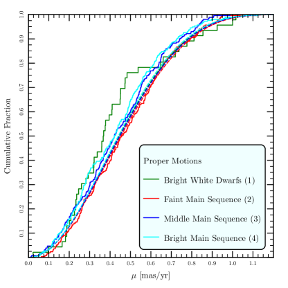
Figure 17.— Cumulative distributions of total proper motion for the subsamples. The observed distributions are given by the solid curves, and the model distributions using the masses in Table 3 are traced by the dashed curves

.

The bright main-sequence stars yield the largest $p-$value in a comparison with the bright white dwarfs of 0.22. The null hypothesis that the bright white dwarfs and the bright main-sequence stars are drawn from the same distribution is the most difficult to reject by these tests. If we suppose that these two groups of stars indeed follow the same underlying proper-motion distribution, we would conclude that the bright WD stars have not yet relaxed to reflect their smaller masses. The observed luminosities of these stars provide constraints on their ages. The median magnitude of the bright-white-dwarf sample is 24.27 in $I-$band with the transformations of Sirianni et al. (2005) from F814W and F606W to $I$. Using the white-dwarf distance of 2.53 kpc (Hansen et al., 2007), a white-dwarf mass of 0.53 M_⊙ (Moehler et al., 2004; Kalirai et al., 2009) and the cooling models of Bergeron et al. (1995) yields a median age of the bright WD sample of 0.5 Gyr. The shorter kinematic distance (see § 4.6) yields a median age of 0.9 Gyr. We will simply take the mean of these two determinations yielding a median age of about 0.7 Gyr.

If the white dwarfs with a median age about 0.7 Gyr have a similar proper-motion distribution to their progenitors even though their masses are substantially less, these stars have not yet relaxed to energy equipartition, and this fact yields a direct estimate of the relaxation time of the cluster in the ACS field. This conclusion agrees with dynamical estimate of the relaxation time for the white dwarfs from Eq. 19 of 1 Gyr at the median projected radius of the subsample, five arcminutes (Fig. 6). Fig. 12 apparently shows that the older white dwarfs have a similar velocity dispersion to the main-sequence stars. The median F814W magnitudes of the next two fainter white-dwarf points are 25.66 and 26.35, corresponding to white-dwarf ages of about 2.5 and 5.2 Gyr respectively (Bergeron et al., 1995), a factor of three to seven older than the bright WD sample. This yields a loose upper limit to the relaxation time in agreement with Eq. 19; however, the errors in proper motions also begin to dominate at these magnitudes, making it difficult to draw conclusions as we must rely more strongly on the subtraction of the observational errors. Better constraints on the proper motions at faint magnitudes from future observations could allow us to place a more reliable upper limit on the relaxation time.

The proper-motion errors increase at faint magnitudes because the poisson noise in the pixels used to determine the position increases as the flux decreases. Brighter than $\mathrm{F814W}=19.5$ saturation begins to set in for the deep images, so a smaller set of shorter exposures is used for the astrometry of brighter stars. The proper-motion errors increase abruptly here and again decrease with brighter magnitudes. This results in a variation of the typical proper motion error for the various samples as shown in Table 3. These errors contribute to the observed dispersions so they have been subtracted from the dispersions in Fig. 12 and 13. They also broaden the cumulative distributions depicted in Fig. 17 and bias the probabilities in Table 4. From Table 3 it is apparent that the typical error in the white dwarfs is substantially larger than for the other samples and that the errors in the other samples are nearly equal to each other; therefore, we artificially increase the proper-motion errors in these samples by adding normally distributed random numbers to each of the proper-motion measurements, so that all four distributions have the same root-mean-square error as the bright white dwarfs. Although the faint-main-sequence sample (FMS) and the white-dwarf sample cover the same range of apparent magnitude, the white dwarfs are typically fainter within that range than the main-sequence stars (see Tab. 3) and hence exhibit larger proper-motion errors.

We then calculate the KS and Wilcoxon probabilities for the new subsamples against the white-dwarf distribution. One thousand new subsamples are generated in this way, and the average probabilities are tabulated. These results are depicted in the column and row labelled “WDN” in Table 4. By making the distributions even broader than the white dwarf distribution, the additional error decreases the $p-$values that result from comparing one sample to another, verifying that the differences in the distributions do not result from differences in the errors.

The distributions depicted in Fig. 17 merit further comment. The faint MS sample appears to have typically larger proper motions than the more massive middle MS sample, and the brightest MS stars have slightly smaller values still. This is in agreement with the values of ${\hat{\sigma}}$ in Table 3 and with the expectations of equipartition. However, from Fig. 5, 12 and 17 we can seen that the velocity dispersions within our field expected from the models vary little with mass (in fact less than is observed), but observations nearer to the core would be a better probe of the dynamical state of the various stars in the cluster.

4.6. The Kinematic Distance of NGC 6397

Fig. 5 depicts the observed proper-motion measurements as a function of distance from the center of the cluster along with the measurements of the radial-velocity dispersion converted to proper motions at a fiducial distance of 2.55 kpc (Richer et al., 2008) and our best-fitting distance of 2 kpc. Leonard & Merritt (1989) argue that for a spherical stellar cluster the proper motions themselves will reveal the hallmark of an anisotropic velocity ellipsoid. In § 4.3 we argue that there is no compelling evidence for anisotropy either in the sample as a whole or in various subsamples; therefore, it is natural to compare the observed proper-motion dispersions with the radial velocity dispersions to obtain a kinematic (or geometric) estimate of the distance to the cluster.

The best-fitting distance with the smallest statistical error in Table 5 is obtained by estimating the proper-motion dispersion of all the main-sequence stars in the proper-motion sample, $0.369\pm 0.009$ mas/yr. We then fit the MM91 data linearly with projected radial distance to estimate the radial-velocity dispersion at the median distance of the stars in our sample (5.16 arcminutes) yielding $3.12\pm 0.11$ km/s. This yields a distance of $1.78\pm 0.07$ kpc. Because it involves the most data, this estimate has the smallest statistical confidence interval. However, there are two possible sources of systematic error that we would like to address. First MM91 actually measured the radial-velocity dispersion at 5.22 arcminutes near the median radius of our dataset to be $3.3\pm 0.8$ km/s. Combining this velocity with the dispersion of the entire dataset yields a larger distance of $1.9\pm 0.5$ kpc. Second, the stars studied by MM91 were among the brightest in the cluster so it is natural to compare the brightest stars in our sample with their data. Fig. 12 shows that the proper-motion dispersion decreases slightly with increasing flux. The dispersion ($\hat{\sigma}$) of the brightest 200 stars in our sample is $0.33^{+0.01}_{-0.03}$ mas/yr with a slightly smaller projected median distance of 5 arcminutes. To obtain a more robust kinematic estimate of the distance to NGC 6397 we have used the unpublished radial velocities from MM91 (Meylan, private communication). We restrict the MM91 dataset to 46 stars with projected distances from the center of NGC 6397 between 3 and 7.2 arcminutes; the median projected distance of this sample from the center is slightly smaller at 4.5 arcminutes. The dispersion of this bright overlap sample is $3.5^{+1.0}_{-0.6}$ km/s after correcting for measurement uncertainties, yielding a distance estimate of $2.2^{+0.5}_{-0.7}$ kpc with a ninety-percent confidence interval. We obtain our best distance estimate by fitting the MM91 data in radius and comparing the dispersion to that of the brightest 200 stars in our sample ($1.9\pm 0.2$ kpc). Additionally we correct for the difference in the median mass of these two samples ($0.84\mathrm{M}_{\odot}$ for the giants and $0.74\mathrm{M}_{\odot}$ for the bright proper motion sample). This yields a distance estimate of $2.0\pm 0.2$ kpc and balances biases against statistical errors. For reference all of these distances are presented in Table 5.

Table 5Distance Estimates to NGC 6397

Method	Value [kpc]	References
Standard-Candle Estimates
Subdwarf fit in $B$ and $V$	$2.53\pm 0.05$	Gratton et al. 2003
Subdwarf fit in $b$ and $y$	$2.58\pm 0.07$	”
Subdwarf fit	$2.67\pm 0.25$	Reid & Gizis 1998
White-dwarf fit	$2.55\pm 0.11$	Hansen et al. 2007
Kinematic Estimates
MS sample (radial fit)	$1.78\pm 0.07$	MM91/Here
MS sample (at 5.22’)	$1.9\pm 0.5$	”
Bright sample (fit)	$1.9\pm 0.2$	”
Bright sample (fit/corr)	$2.0\pm 0.2$	”
Bright overlap sample	$2.2^{+0.5}_{-0.7}$	”

These successive distance estimates trade larger statistical errors for reduced systematic errors that arise from the heterogeneity of the stars and through interpolating the velocity profiles in radius. The final estimate of $2.2^{+0.5}_{-0.7}$ kpc compares stars of nearly the same mass at the same median radius, so it minimizes the systematic errors; however, it uses only a portion of both samples, so the statistical errors are necessarily larger. Increasing the size of the sample of stars with radial-velocity measurements could dramatically decrease the uncertainities of this kinematic distance estimate.

4.7. The Mass of NGC 6397

Leonard & Merritt (1989) outlined several mass estimators for the open cluster M35 using the observed proper-motions. Among these the most straightforward is

$$\langle GM_{r}\rangle=\frac{16}{\pi}\left\langle R\left(\frac{2}{3}v_{R}^{2}+\frac{1}{3}v_{T}^{2}\right)\right\rangle$$ (21)

where $v_{R}$ is the component of the proper-motion toward the center of the cluster and $v_{T}$ is the tangential component of the proper-motion. This estimator yields

$$M_{r}=8.3\pm 0.4\times 10^{4}d_{2.53}^{3}\mathrm{M}_{\odot}$$ (22)

where we have summed over all of the stars along the cluster main sequence and white-dwarf cooling tracks and excluded those stars with proper motion errors greater than 0.4 mas/yr or proper-motions greater than 5 mas/yr. The confidence interval gives a ninety-percent confidence region obtained through bootstrapping the sample.

We use the power-law fits to the column density and velocity dispersion (Eq. 16) of the cluster to deproject the proper-motion dispersion, density and their gradients to obtain an estimate of the mass enclosed within the outer radius of our field. We can simply apply Jeans equation

$$v_{r}^{2}-\sigma_{r}^{2}\left[\frac{d\ln\sigma_{r}^{2}}{d\ln r}+\frac{d\ln n}{d\ln r}+\beta\right]=\frac{GM_{r}}{r}$$ (23)

to obtain an estimate of the enclosed mass within a given spherical radius ($M_{r}$). The symbols $\sigma_{r}$ and $n$ denote the radial velocity dispersion and the number density of stars. In this equation $v_{r}$ and $\beta$ quantify the rotation of the cluster and the anisotropy of the velocity distribution; we see evidence for neither in our data, so we assume these vanish to yield

$$M_{r}=8.7\pm 0.6\times 10^{4}d_{2.53}^{3}\left(\frac{R}{7^{\prime}}\right)^{0.6}\mathrm{M}_{\odot}.$$ (24)

Whether one uses $\sigma$ or $\hat{\sigma}$ in Eq. 23 does not affect the mass estimate (Eq. 24) within the errorbars. We used proper motions and positions themselves without binning in radius to determine the best fitting power-law relations (Eq. 17) for the column density and velocity dispersion, yielding a mass estimate of

$$M_{r}=8.5\pm 0.6\times 10^{4}d_{2.53}^{3}\left(\frac{R}{7^{\prime}}\right)^{0.64}\mathrm{M}_{\odot}.$$ (25)

We can combine these estimates with the light within this projected radius to yield

$$L_{V,R}=4.0\times 10^{4}d_{2.53}^{2}\mathrm{L}_{V,\odot}$$ (26)

and the model for the light distribution outlined in § 4.1 allows us to estimate the luminosity within the spherical radius at

$$L_{V,r}=3.5\times 10^{4}d_{2.53}^{2}\mathrm{L}_{V,\odot}$$ (27)

Scaling the mass within seven arcminutes (Eq. 25) by the ratio of the total light (Table 1) to that within seven arcminutes (Eq. 27) yields an estimate of the total mass of the cluster of

$$M=1.1\pm 0.1\times 10^{5}d_{2.53}^{3}\mathrm{M}_{\odot}$$ (28)

in agreement with the model mass (Eq. 12) found in § 4.1. This gives a mass-to-light ratio of $2.4\pm 0.3d_{2}\mathrm{M}_{\odot}/\mathrm{L}_{V,\odot}$; including the uncertainty in the distance yields $2.4\pm 0.5\mathrm{M}_{\odot}/\mathrm{L}_{V,\odot}$. This agrees with the previous result of MM91 of $2.1\pm 0.1$ at an assumed distance of 2.4 kpc. The mass-to-light ratio of the totality of the stellar population of NGC 6397 range from 1.4 to 2.0 according to MM91 and about 1.2 according to Drukier (1995). Our present mass-to-light measurement does not require any dark contribution to the mass of NGC 6397.

4.8. Stellar Escapers

Fig. 5 also depicts the escape velocity as a function of distance from the center of the cluster. The escape velocity (here given as an escape proper-motion) is about three times the velocity dispersion for the range of radii probed by the observations. This is the escape velocity at a given distance (not projected) from the center of the cluster; therefore, a star with a proper-motion larger than this at a particular projected radius will escape. Exceeding this proper-motion is a sufficient condition for escape. Other stars whose actual three-dimensional distances are further from the cluster center may also escape as can stars with significant motion along the line of sight. For an isotropic velocity distribution the three-dimensional velocity is typically only about twenty percent larger than the proper-motion; therefore, we will use a conservative criterion and consider stars that exceed the escape proper-motion as potential escapers.

Table 6Cluster stars with proper-motions that exceed the local escape proper motion

			$\mu_{\mathrm{tot}},\mu_{e}$	$\alpha_{2000}$	$\delta_{2000}$	$\mu_{\alpha}$	$\mu_{\delta}$	$\mu_{R}$
ID	F814W	F606W-F814W	[mas yr-1]	[arcsec]	[arcsec]	[mas yr-1]	[mas yr-1]	[mas yr-1]	Comment
14960	18.92	1.03	1.27, 1.10	40.38	84.95	1.24$\pm$0.08	-0.28$\pm$0.08	$0.77\pm 0.08$	MS, short
35641	18.93	1.00	1.52, 1.15	33.10	167.75	1.16$\pm$0.05	-0.98$\pm$0.05	$1.00\pm 0.05$	MS, short
39398	18.93	1.02	1.32, 1.13	71.20	180.95	1.17$\pm$0.08	-0.62$\pm$0.08	$1.00\pm 0.08$	MS, short
34104	19.04	1.04	1.41, 1.15	33.82	162.30	1.30$\pm$0.05	-0.56$\pm$0.05	$0.95\pm 0.05$	MS, short
16272	19.27	1.08	1.12, 1.10	35.40	91.00	0.81$\pm$0.03	0.76$\pm$0.03	$-0.11\pm 0.03$	MS, short
25395	21.12	1.38	1.34, 1.11	70.85	129.75	1.26$\pm$0.01	0.44$\pm$0.01	$0.48\pm 0.01$	MS
14687	23.42	1.98	1.11, 1.06	134.25	83.70	-0.32$\pm$0.05	-1.06$\pm$0.05	$0.41\pm 0.05$	MS
19308	25.67	0.74	1.10, 1.08	96.95	102.95	-0.16$\pm$0.21	-1.09$\pm$0.21	$0.56\pm 0.21$	WD
21043	26.14	0.91	1.32, 1.10	68.60	112.45	-0.74$\pm$0.35	1.09$\pm$0.35	$-0.98\pm 0.35$	WD
27645	26.18	0.96	1.19, 1.07	137.35	139.00	-1.18$\pm$0.27	-0.14$\pm$0.27	$-0.77\pm 0.27$	WD
34340	26.23	0.93	1.26, 1.11	90.70	163.20	-1.10$\pm$0.33	-0.61$\pm$0.33	$-0.46\pm 0.33$	WD
9666	26.29	0.96	1.21, 1.08	48.60	59.70	1.07$\pm$0.32	-0.56$\pm$0.32	$0.89\pm 0.32$	WD
15213	26.30	1.01	1.12, 1.04	184.80	86.15	-0.95$\pm$0.36	0.59$\pm$0.36	$-1.00\pm 0.36$	WD
4333	26.39	1.07	1.29, 1.08	10.77	30.96	-0.93$\pm$0.33	-0.90$\pm$0.33	$0.30\pm 0.33$	WD
28585	26.40	1.05	1.32, 1.14	23.43	142.55	1.14$\pm$0.36	-0.66$\pm$0.36	$0.95\pm 0.36$	WD
25008	26.44	1.03	1.45, 1.05	181.60	128.10	0.12$\pm$0.26	-1.44$\pm$0.26	$0.57\pm 0.26$	WD
3445	26.54	1.14	1.37, 1.07	20.72	25.39	0.55$\pm$0.31	1.25$\pm$0.31	$-0.62\pm 0.31$	WD
30992	26.55	1.12	1.30, 1.07	141.70	151.00	0.94$\pm$0.28	-0.90$\pm$0.28	$0.97\pm 0.28$	WD
433	26.61	1.22	1.35, 1.03	123.15	6.78	0.63$\pm$0.37	1.19$\pm$0.37	$-0.38\pm 0.37$	WD
27465	26.62	1.18	1.55, 1.08	120.70	138.20	1.19$\pm$0.35	1.00$\pm$0.35	$0.27\pm 0.35$	WD
31935	26.65	1.16	1.30, 1.15	24.08	154.50	0.81$\pm$0.28	-1.02$\pm$0.28	$0.99\pm 0.28$	WD
16969	26.67	1.20	1.52, 1.10	42.69	93.90	-0.57$\pm$0.34	-1.40$\pm$0.34	$0.49\pm 0.34$	WD
30725	26.72	1.27	1.42, 1.06	176.30	150.00	0.54$\pm$0.30	1.31$\pm$0.30	$-0.09\pm 0.30$	WD
25724	27.00	1.26	1.65, 1.06	163.30	131.10	0.26$\pm$0.39	1.62$\pm$0.39	$-0.38\pm 0.39$	WD

The quantities $\alpha_{2000}$ and $\delta_{2000}$ give the offset in arcseconds from the origin of the coordiates of the field at $\alpha=17^{\mathrm{h}}40^{\mathrm{m}}56^{\mathrm{s}}\!\!.72$ and $\delta=-53^{\circ}45^{\prime}36^{\prime\prime}\!\!.8$.

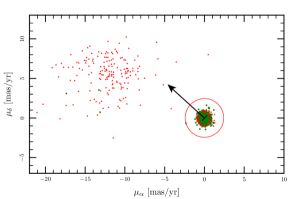
Figure 18.— Proper motions of the objects identified as stars in the ACS field and lying near the main sequence and white dwarf cooling track of NGC 6397. The mean proper-motion of the cluster members has been subtracted. The red circle denotes twice the escape proper-motion from the inner edge of the ACS field.

Fig. 18 depicts the proper motions of all stars along the main-sequence and white-dwarf tracks. The tight cloud centered near zero proper motion are the cluster members whereas the more diffuse cloud at $\mu_{\alpha}\approx-12$ mas/yr consists of field stars that happen to have fluxes similar to cluster main-sequence or white-dwarf stars. A comparison with the proper motions of all stellar sources in Fig. 1 demonstrates that the flux criteria removes nearly all the field stars while affecting the potential cluster stars more modestly. We define the region of potential escapers as having a total proper motion between once and twice the escape proper motion for stars at the inner edge of the ACS field. This upper limit is indicated by the red circle. Looking at the density of presumably field stars outside this circle, one expects fewer than one field star within the narrow range of color and proper motion.

Table 6 lists those stars that lie on or near the cluster main-sequence or white-dwarf tracks whose total proper motion exceeds the escape proper motion at the tangent point for the projected radius of the star. We have verified that all of these potential escapers satisfy the image-quality criteria outlined in Anderson et al. (2008). Fig. 19 depicts the ratios of the stellar proper motions to the escape proper motion (Tab 6 lists those stars between the two circles). Looking at the proper motions themselves in Fig. 19, the potential white-dwarf escapers (green) appear to be a smooth extension of the rest of the stars; whereas the potential main-sequence (red) escapers appear to lie beyond the tail of the main-sequence distribution. The positions of the potential escapers in Fig. 20 do not appear extraordinary; however, their locations on the color-magnitude diagram in Fig. 21 are. The potential escaping white dwarfs are among the faintest stars with measured proper motions in the sample and therefore are prone to greater error. This agrees well with the apparent smoothness of their proper-motion distribution with the rest of the white-dwarf population.

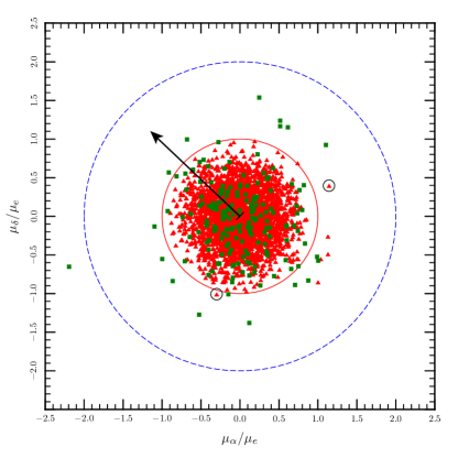
Figure 19.— The proper motions of potential stellar escapers. Only objects with proper-motion errors less than 0.4 mas/yr are included (the minimum escape proper motion is 1.3 mas/yr). There is no proper-motion cutoff. The arrow indicates the direction of the center of the cluster. The proper motions of stars along the main sequence and white-dwarf track are depicted with red triangles and green squares respectively. The most likely escapers are circled. The escape proper motion is denoted by the solid red circle and twice its value by the dashed blue circle.

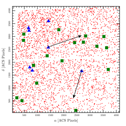
Figure 20.— The positions of potential stellar escapers. The center of the cluster is located beyond the upper-left corner of the field. The red dots show the positions of all stars in the sample, the potential escaping MS stars are blue triangles, and potential escaping WD stars are green squares. The motions of two most likely escapers over the next fifty thousand years are depicted.

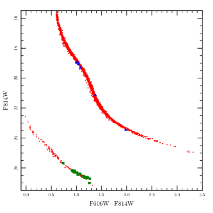
Figure 21.— The color and magnitude of potential stellar escapers. The red dots show the positions of all stars in the sample, the potential escaping MS stars are blue triangles, and WD stars are green squares.

On the other hand, the location of the potential main-sequence escapers in Fig. 21 presents a bit more of a puzzle. All but two of these stars lie between $18.9<\mathrm{F814W}<19.3$ where the astrometry begins to use the shorter exposures in which these stars are not saturated. In fact in these short exposures the proper-motion errors are comparable to those of $\mathrm{F814W}\approx 24$ in the longer exposures and approach 0.1 mas/yr. Although these errors are not as large as those for the potential white-dwarf escapers, there are many more stars at these magnitudes, so one would expect a number of outliers. The final potential escapers lie at $\mathrm{F814W}\approx 21$ and 23 where the proper-motion errors are typically less than 0.05 mas/yr. Statistically it is unlikely that these objects are field stars for the reasons mentioned earlier. The brighter, faster moving star (ID 25395) with a total proper motion of 1.34 mas/yr appears clearly beyond the tail in the distribution shown in Fig. 16. From Tab. 6 we see that its total proper motion exceeds its escape proper motion by sixteen times its proper-motion error. On the other hand the fainter, slower moving star (ID 14687) exceeds its escape proper motion by about the value of its proper motion error, so its assignment as an escaper is less certain. In fact given the number of stars slightly below the escape threshold it is likely that this star is not an escaper but rather measurement errors pushed it above the threshold; therefore, we estimate that there is one escaper out of a sample of 3,245 stars. Typically a star on an escape trajectory will leave the cluster within a crossing time, $\tau_{c}\sim r/v\approx 5^{\prime}/0.3~{}\mathrm{mas~{}yr}^{-1}\approx 10^{6}$ yr. This yields an estimate of the evaporation timescale, $(d\ln N/dt)^{-1}\approx 3$ Gyr, or about three relaxation timescales. This evaporation timescale does not indicate that the cluster will vanish over the next 2 Gyr. On the contrary the escaping stars as apparent from Fig. 21 are less massive than average so the mass-loss timescale will be perhaps two or three times longer; furthermore, this timescale is the time over which the cluster loses about two-thirds of its stars, not all of them. This agrees with the destruction timescale calculated by (Gnedin & Ostriker, 1997) of about 4 Gyr. This star is moving away from the centre of the cluster, although it does not travel on a strictly radial trajectory. This is not surprising as the diffusion of stars in velocity to become unbound is not dominated by a few strong encounters but by many small ones. The final of these small encounters could have occurred anywhere within the cluster not necessarily near the centre, so the trajectory of a star as it escapes need not be radial.

5. Discussion

5.1. Dynamics

The proper motion measurements by ACS in NGC 6397 reveal gross agreement with the features of a mass-segregated lowered isothermal distribution function for the stars. On the face of it this conclusion is not particularly surprising because such a model was conceived to describe globular clusters such as NGC 6397. There is no strong evidence for anisotropy in the proper motion distribution, neither in the stellar population as a whole nor in subsamples of stars of particular apparent magnitude or at particular projected distances from the cluster center.

Three discrepancies with the lowered isothermal distribution are apparent. First, the effects of mass segregation appear larger in the data than predicted in the model under the assumption that $m_{i}\sigma_{i}^{2}$ is constant. The velocity dispersion in the ACS field depends modestly on the apparent magnitude (the mass) of the stars, as expected for the model; however, the mass dependence appears to be slightly stronger in the data than in our model (Fig. 12). Furthermore, the radial distribution of stars in our sample depends more strongly on mass than in the models (Fig. 6); these differences are stronger than we expect from incompleteness (Fig. 7). Second, the proper motion distribution of young white dwarfs (younger than 0.7 Gyr) appear to not satisfy equipartition with the other stars of the cluster. Their proper motions are probably smaller than those of stars of similar masses, and their proper motions are most similar to the motions of the most massive stars observed in the cluster, i.e. stars similar to their progenitors. The young white dwarfs do not appear to have relaxed, yielding the first direct measurement of the relaxation time in a globular cluster of about or greater than 0.5 Gyr. This value agrees with the theoretical expectations from the number of stars in NGC 6397 near the half-light radius and the velocity dispersion of the cluster. Thirs, there are some stars with sufficient energy to escape the cluster whereas the lowered isothermal distribution function contains no escaping stars. The abundance of these stars along with the observed crossing time yields an estimate of the evaporation time of the cluster of about 3 Gyr. Because the typical escaping stars have masses smaller than average, the mass-loss timescale is longer perhaps by a factor of a few. This constraint agrees with theoretical expectations (Gnedin & Ostriker, 1997) of a destruction timescale of about 4 Gyr.

5.2. Properties

Because the ACS field lies beyond the half-light radius of the cluster, the measurements yield an estimate for the total mass of the globular cluster with only modest extrapolation. The resulting mass is $1.1\pm 0.1\times 10^{5}d_{2.53}^{3}\mathrm{M}_{\odot}$ in agreement with the result of MM91. Proper motions, unlike radial velocity measurements, probe the isotropy of the velocity distribution, so they give a more robust mass estimate (Leonard & Merritt, 1989). Because the proper motions show no evidence for anisotropy, the line-of-sight velocity measurements of MM91 who assumed isotropy gave a similar mass estimate and mass-to-light estimate. This mass-to-light ratio (of about 1.5 in solar units) does not indicate a need for dark matter in the cluster to explain the observed dynamics.

The major difference with previous results is the kinematic estimate of the distance to NGC 6397. These estimates range from $1.78\pm 0.07$ kpc to $2.2^{+0.5}_{-0.7}$ kpc as summarized in Table 5. The larger estimates mitigate against various known biases at the expense of increased statistical uncertainties. Our best estimate with the current data of $2.0\pm 0.2$ kpc with ninety-percent confidence was obtained by fitting a linear model to the radial velocity dispersion measured by MM91 and comparing this with the dispersion of the proper motions of the brightest stars in our sample and by correcting for the difference in mass between the bright-star sample and the giants. Although our longest distance (and most uncertain) estimate does agree with the previous standard-candle estimates, the most precise of which is $2.53\pm 0.05$ kpc within their individual ninety-percent confidence intervals, there is some tension between our best estimate ($2.0\pm 0.2$ kpc) and the standard-candle estimates. A short kinematic distance to NGC 6397 is similar to the short distance found by MAM06 for 47 Tuc that was also about twenty percent smaller than the standard candle estimates. This kinematic distance estimate is still plagued by potential systematic errors because the stars with proper motions are not the stars with radial velocities; therefore, some extrapolation over position in the cluster and stellar mass is required to get the distance estimate. Such a short distance, if indeed correct, could pose a challenge for stellar evolution and white dwarf cooling models; however, it does indicate a need to obtain more precise and model-independent measurements of distances to globular clusters.

5.3. Future Directions

In light of the data presented, further modelling of the cluster is warranted. In particular a larger $N-$body model than that recently performed by Hurley et al. (2008) to account for both the observed star count and the observed proper motions could dramatically increase our understanding of this well-studied cluster. In particular the improved model of the cluster should include the effects of disk shocking to consider the effects of the observed orbit (Kalirai et al., 2007) of the cluster. As mentioned in the introduction, the number of the stars in the outskirts of the Hurley et al. (2008) model were insufficient for a detailed comparison with the data. A model resulting in a final cluster with more than 150,000 stars would be sufficient for a comparison in this field. An observational study closer to the core of NGC 6397 would be easier to compare with numerical models because the higher stellar densities both in the models and the data may allow a detailed comparison with current models. Combination of the outer and the inner observations for this cluster or 47 Tuc would be important. Our attempts to obtain a kinematic estimate of the distance to NGC 6397 have been thwarted by potential systematic errors in particular, a lack of overlap between the stars with proper motions (presented here) and those with radial velocities (MM91). This obstacle also affected the work of MAM06 for 47 Tuc. A natural way forward would be to obtain radial velocity measurements for the brightest stars in our proper motion sample with F814W $\sim 16$. This would yield the first significant sample of stars with known velocities in all three directions for a globular cluster and would prove a powerful tool in probing the cluster as well as obtaining a distance estimate.

Given the relative vicinity of NGC 6397 to Earth (and 47 Tuc as well for that matter) and the high-precision astrometry of ACS, a natural next step would be to measure the distances to these clusters with parallax. Both astrometric epochs for this work were obtained at the same time of year, removing the effects of parallax to focus on the proper motion of the cluster and its stars. Kalirai et al. (2007) found a sufficient number of background galaxies to fix the astrometry to a precision of about 0.2 mas. Even with ACS observations at a different time of year, this level of precision is insufficient to improve on the current precision of the measurement of the distance to NGC 6397. Two potential ways forward would be to find another way to fix the astrometry or to obtain proper motions and radial velocities for the same stars. In the more distant future GAIA should be able to measure the distance to NGC 6397 and other nearby clusters. Distances to these nearby metal-rich and metal-poor clusters would have dramatic implications beyond the study of globular clusters themselves from detailed stellar models to the extragalactic distance ladder, extending to the edge of the observable Universe.

The observations presented here probe beyond the half-light radius of NGC 6397. In particular a useful approximation is the limit where the value of $v_{e}\ll\sigma$ as is appropriate in this region. In this limit we have

$$J_{n}\approx\frac{1}{\sigma^{2}}\int_{0}^{v_{e}}\frac{v_{e}^{2}-v^{2}}{2}v^{n+2}dv\approx\frac{1}{\sigma^{2}}\frac{v_{e}^{n+5}}{(n+3)(n+5)}$$ (A1)

so ratios such as $\langle v^{2}\rangle=J_{2}/J_{0}$ no longer depend on $\sigma$. This particular limit applies near the edge of the cluster regardless of the underlying distribution function as long as the distribution function is approximately linear in energy near the escape threshold. Furthermore, the linear approximation of the distribution function underestimates the number of stars with small velocities; therefore, it will overestimate the value of higher moments of the distribution function relative to lower ones. In particular

$$\langle v^{2}\rangle=\frac{3}{7}v_{e}^{2}~{}\mathrm{or}~{}\langle v_{1D}^{2}\rangle=\frac{v_{e}^{2}}{7}$$ (A2)

yielding an estimate of the escape velocity in terms of the local one-dimensional velocity dispersion. Let us define the line-of-sight integrated quantities

$$K_{n}(R)\equiv\int_{-\infty}^{\infty}J_{n}dz=2\int_{0}^{\pi/2}\!\!J_{n}(R\sec\theta)\sec^{2}\theta d\theta\approx 2\int_{0}^{\pi/2}\frac{1}{\sigma^{2}}\frac{v_{e}^{n+5}}{(n+3)(n+5)}\sec^{2}\theta d\theta.$$ (A3)

Let us assume that the bulk of the matter lies within the radius $R$, so

$$\Psi=\frac{v_{e}^{2}}{2}\approx\frac{GM}{r}-\frac{GM}{r_{t}}=\frac{GM}{R}\left(\cos\theta-\cos\theta_{t}\right)$$ (A4)

where $\cos\theta_{t}=R/r_{t}$, so in this limit

$$K_{n}(R)\approx\frac{2}{\sigma^{2}}\frac{\left(2GM/R\right)^{(n+5)/2}}{(n+3)(n+5)}\int_{0}^{\theta_{t}}\frac{\left(\cos\theta-\cos\theta_{t}\right)^{(n+5)/2}}{\cos^{2}\theta}d\theta.$$ (A5)

If $R\ll r_{t}$ we get

$$K_{n}(R)=\frac{\pi^{1/2}}{\sigma^{2}}\frac{v_{e}(R)^{n+5}}{(n+3)(n+5)}\frac{\Gamma\left(\frac{n+3}{4}\right)}{\Gamma\left(\frac{n+5}{4}\right)}$$ (A6)

so

$$v_{e}(R)\approx\frac{\Gamma^{2}\left(\frac{3}{4}\right)}{\pi}\sqrt{42\langle v_{1D}^{2}\rangle_{\mathrm{LOS}}}\approx 3.1\sqrt{\langle v_{1D}^{2}\rangle_{\mathrm{LOS}}}.$$ (A7)

As the ratio of the projected radius to the tidal radius increases, $v_{e}(R)$ approaches $\sqrt{8}\sqrt{\langle v_{1D}^{2}\rangle_{\mathrm{LOS}}}$. This not only provides a useful empirical estimator of the local escape velocity to find stars that may be escaping but also demonstrates that the observed velocity dispersion integrated along the line of sight for the outer regions of the cluster is independent of the value of $\sigma$; therefore, it is also independent of the mass of the stars even if equipartition holds and $\sigma\propto m^{-1/2}$. Further examination of Eq. A1 and A6 shows that the density of stars in the outskirts of the cluster is proportional to $\sigma^{-2}$ but the radial dependence is independent of the value of $\sigma$; therefore, within a field where $v_{e}\ll\sigma$ we expect that the signatures of mass segregation will be weaker than regions where $v_{e}\gtrsim\sigma$.

This paper looks at the distribution of the magnitude of proper motions that results from integrating the phase-space density over the allowed range of velocities along the line of sight,

$$n_{2}(v|r)=\frac{\rho_{1}}{2\pi\sigma^{2}}~{}\mathrm{erf}\left(\sqrt{\frac{v^{2}_{e}-v^{2}}{2\sigma^{2}}}\right)e^{(v_{e}^{2}-v^{2})/(2\sigma^{2})}-\frac{2\rho_{1}\sqrt{v^{2}_{e}-v^{2}}}{\left(2\pi\sigma^{2}\right)^{3/2}}$$ (A8)

where $\rho_{1}$ is a normalizing factor. Of particular interest is the cumulative distribution of the magnitude of the proper motion of the stars. The number density of stars with proper motions greater than a given value $v$ is

$$n(>v|r)=\rho_{1}\Biggr{[}\exp\left(\frac{v^{2}_{e}-v^{2}}{2\sigma^{2}}\right)\mathrm{erf}\left(\sqrt{\frac{v^{2}_{e}-v^{2}}{2\sigma^{2}}}\right)-\sqrt{\frac{2}{\pi}\frac{v_{e}^{2}-v^{2}}{\sigma^{2}}}\left(1+\frac{v_{e}^{2}-v^{2}}{3\sigma^{2}}\right)\Biggr{]}.$$ (A9)

One should note that one can get Eq. A9 simply by replacing $v_{e}$ in Eq. 3 (of the main text) with $\sqrt{v_{e}^{2}-v^{2}}$; therefore, in the limit as the minimum velocity $v$ vanishes, Eq. A9 yields Eq. 3 as expected. The observable is of course the velocity distribution of the sample along the line of sight

$$N(>v|R)=\int_{R}^{r_{t}}n(>v|r)\frac{rdr}{\sqrt{r^{2}-R^{2}}},$$ (A10)

which must be calculated numerically. Alternatively we can integrate $n(>v|r)$ against the spherical window function defined in § 3.2 to obtain the proper-motion distribution for the entire field.

References

- Anderson & Bedin (2010) Anderson, J. & Bedin, L. R. 2010, PASP, 122, 1035
- Anderson & King (2006) Anderson, J. & King, I. R. 2006, PSFs, Photometry, and Astronomy for the ACS/WFC, Tech. rep., Space Telescope Science Institute
- Anderson et al. (2008) Anderson, J., King, I. R., Richer, H. B., Fahlman, G. G., Hansen, B. M. S., Hurley, J., Kalirai, J. S., Rich, R. M., & Stetson, P. B. 2008, AJ, 135, 2114
- Anderson & Darling (1952) Anderson, T. W. & Darling, D. A. 1952, Ann. Math. Statist., 193
- Bergeron et al. (1995) Bergeron, P., Wesemael, F., & Beauchamp, A. 1995, PASP, 107, 1047
- Cardelli et al. (1989) Cardelli, J. A., Clayton, G. C., & Mathis, J. S. 1989, ApJ, 345, 245
- D’Antona et al. (2005) D’Antona, F., Bellazzini, M., Caloi, V., Pecci, F. F., Galleti, S., & Rood, R. T. 2005, ApJ, 631, 868
- Davis et al. (2008a) Davis, D. S., Richer, H. B., Anderson, J., Brewer, J., Hurley, J., Kalirai, J. S., Rich, R. M., & Stetson, P. B. 2008a, AJ, 135, 2155
- Davis et al. (2008b) Davis, D. S., Richer, H. B., King, I. R., Anderson, J., Coffey, J., Fahlman, G. G., Hurley, J., & Kalirai, J. S. 2008b, MNRAS, 383, L20
- di Criscienzo et al. (2010) di Criscienzo, M., D’Antona, F., & Ventura, P. 2010, A&A, 511, A70
- Dotter et al. (2007) Dotter, A., Chaboyer, B., Jevremović, D., Baron, E., Ferguson, J. W., Sarajedini, A., & Anderson, J. 2007, AJ, 134, 376
- Drukier (1995) Drukier, G. A. 1995, ApJS, 100, 347
- Efron (1979) Efron, B. 1979, Ann. Stat., 7, 1
- Ford et al. (1998) Ford, H. C. et al. 1998, in Presented at the Society of Photo-Optical Instrumentation Engineers (SPIE) Conference, Vol. 3356, Society of Photo-Optical Instrumentation Engineers (SPIE) Conference Series, ed. P. Y. Bely & J. B. Breckinridge, 234–248
- Giersz & Heggie (2009) Giersz, M. & Heggie, D. C. 2009, MNRAS, 395, 1173
- Gnedin et al. (1999) Gnedin, O. Y., Lee, H. M., & Ostriker, J. P. 1999, ApJ, 522, 935
- Gnedin & Ostriker (1997) Gnedin, O. Y. & Ostriker, J. P. 1997, ApJ, 474, 223
- Goldsbury et al. (2010) Goldsbury, R., Richer, H. B., Anderson, J., Dotter, A., Sarajedini, A., & Woodley, K. 2010, AJ, 140, 1830
- Goldsbury et al. (2011) —. 2011, AJ, 142, 66
- Gratton et al. (2003) Gratton, R. G., Bragaglia, A., Carretta, E., Clementini, G., Desidera, S., Grundahl, F., & Lucatello, S. 2003, A&A, 408, 529
- Hansen et al. (2007) Hansen, B. M. S. et al. 2007, ApJ, 671, 380
- Harris (1996) Harris, W. E. 1996, AJ, 112, 1487, (2010 edition)
- Heggie & Giersz (2008) Heggie, D. C. & Giersz, M. 2008, MNRAS, 389, 1858
- Heggie & Giersz (2009) —. 2009, MNRAS, 397, L46
- Hurley et al. (2008) Hurley, J. R., Shara, M. M., Richer, H. B., King, I. R., Saul Davis, D., Kalirai, J. S., Hansen, B. M. S., Dotter, A., Anderson, J., Fahlman, G. G., & Rich, R. M. 2008, AJ, 135, 2129
- Kalirai et al. (2007) Kalirai, J. S., Anderson, J., Richer, H. B., King, I. R., Brewer, J. P., Carraro, G., Davis, S. D., Fahlman, G. G., Hansen, B. M. S., Hurley, J. R., Lépine, S., Reitzel, D. B., Rich, R. M., Shara, M. M., & Stetson, P. B. 2007, ApJ, 657, L93
- Kalirai et al. (2008) Kalirai, J. S., Hansen, B. M. S., Kelson, D. D., Reitzel, D. B., Rich, R. M., & Richer, H. B. 2008, ApJ, 676, 594
- Kalirai et al. (2009) Kalirai, J. S., Saul Davis, D., Richer, H. B., Bergeron, P., Catelan, M., Hansen, B. M. S., & Rich, R. M. 2009, ApJ, 705, 408
- King (1966) King, I. R. 1966, AJ, 71, 64
- Kuiper (1960) Kuiper, N. H. 1960, Proceedings of the Koninklijke Nederlandse Akademie van Wetenschappen, Series A, 63, 38
- Leonard & Merritt (1989) Leonard, P. J. T. & Merritt, D. 1989, ApJ, 339, 195
- Lind et al. (2011) Lind, K., Charbonnel, C., Decressin, T., Primas, F., Grundahl, F., & Asplund, M. 2011, A&A, 527, A148
- Lupton (1993) Lupton, R. 1993, Statistics in theory and practice (Princeton, N.J.: Princeton University Press)
- McLaughlin et al. (2006) McLaughlin, D. E., Anderson, J., Meylan, G., Gebhardt, K., Pryor, C., Minniti, D., & Phinney, S. 2006, ApJS, 166, 249, (MAM06)
- Meylan & Mayor (1991) Meylan, G. & Mayor, M. 1991, A&A, 250, 113, (MM91)
- Michie (1963) Michie, R. W. 1963, MNRAS, 126, 499
- Milone et al. (2008) Milone, A. P., Bedin, L. R., Piotto, G., Anderson, J., King, I. R., Sarajedini, A., Dotter, A., Chaboyer, B., Marín-Franch, A., Majewski, S., Aparicio, A., Hempel, M., Paust, N. E. Q., Reid, I. N., Rosenberg, A., & Siegel, M. 2008, ApJ, 673, 241
- Milone et al. (2011) Milone, A. P., Marino, A. F., Piotto, G., Bedin, L. R., Anderson, J., Aparicio, A., Cassisi, S., & Rich, R. M. 2011, ArXiv e-prints
- Moehler et al. (2004) Moehler, S., Koester, D., Zoccali, M., Ferraro, F. R., Heber, U., Napiwotzki, R., & Renzini, A. 2004, A&A, 420, 515
- Pryor et al. (1986a) Pryor, C., Hartwick, F. D. A., McClure, R. D., Fletcher, J. M., & Kormendy, J. 1986a, AJ, 91, 546
- Pryor et al. (1986b) Pryor, C., Smith, G. H., & McClure, R. D. 1986b, AJ, 92, 1358
- Ratnatunga & Bahcall (1985) Ratnatunga, K. U. & Bahcall, J. N. 1985, ApJS, 59, 63
- Reid & Gizis (1998) Reid, I. N. & Gizis, J. E. 1998, AJ, 116, 2929
- Richer et al. (2006) Richer, H. B., Anderson, J., Brewer, J., Davis, S., Fahlman, G. G., Hansen, B. M. S., Hurley, J., Kalirai, J. S., King, I. R., Reitzel, D., Rich, R. M., Shara, M. M., & Stetson, P. B. 2006, Science, 313, 936
- Richer et al. (2008) Richer, H. B. et al. 2008, AJ, 135, 2141
- Rousseeuw & Croux (1993) Rousseeuw, P. J. & Croux, C. 1993, Journal of the American Statistical Association, 88, 1273
- Sirianni et al. (2005) Sirianni, M. et al. 2005, PASP, 117, 1049
- Spitzer (1987) Spitzer, L. 1987, Dynamical Evolution of Globular Clusters, Princeton Series in Astrophysics (Princeton: Princeton)
- Spitzer & Hart (1971) Spitzer, Jr., L. & Hart, M. H. 1971, ApJ, 164, 399
- Trager et al. (1995) Trager, S. C., King, I. R., & Djorgovski, S. 1995, AJ, 109, 218