Isolated prompt photon pair production at hadron colliders with $k_{T}$-factorization

Abstract

In the framework of the $k_{T}$-factorization approach, the isolated prompt photon pair production in $pp$ and $p\bar{p}$ collisions at high energies is studied. The consideration is based on the quark-antiquark annihilation, quark-gluon scattering and gluon-gluon fusion subprocesses, where the non-zero transverse momenta of incoming partons are taken into account. The unintegrated quark and gluon densities in a proton are determined using the Kimber-Martin-Ryskin prescription. The numerical analysis covers the total and differential production cross sections and extends to specific angular correlations between the produced prompt photons. Theoretical uncertainties of our evaluations are studied and comparison with the NLO pQCD calculations is performed. The numerical predictions are compared with the recent experimental data taken by the D$\emptyset$, CDF, CMS and ATLAS collaborations at the Tevatron and LHC energies.

PACS number(s): 12.38.-t, 13.60.Hb, 13.85.Qk

1 Introduction

The production of prompt photon pairs in hadronic collisions at high energies is of great interest at present[1, 2, 3, 4, 5]. It provides a major background to searches for rare or exotic processes in both the Tevatron and the LHC. In particular, it represents a major source of large and irreducible background to searches for the Higgs boson in the low mass range, where its first indications (with mass of about 125–126 GeV) have been found very recently. It is also a significant background to searches for a new heavy resonances[6], cascade decays of a new heavy particles[7] and to searches for some effects of physics beyond the Standard Model. For example, so called Universal Extra-Dimensions predict non-resonant diphoton production associated with significant missing transverse energy[8, 9]. Other extra-dimension models, such as Randall-Sundrum model[10], predict the production of gravitons, which would decay into photon pairs with a narrow width. From another side, studies of prompt diphoton production provide a particularly clean test of perturbative Quantum Chromodynamics (pQCD) and soft-gluon resummation methods implemented in theoretical calculations since the produced photons are largely insensitive to the effects of final-state hadronization, and their energies and directions can be measured with high precision. Therefore, it is essential to have an accurate pQCD predictions for corresponding cross sections and related kinematical distributions.

The leading contributions to the production of prompt photon pairs at hadron collisions are the quark-antiquark annihilation $q\bar{q}\to\gamma\gamma$, gluon-gluon fusion $gg\to\gamma\gamma$ and quark-gluon scattering $qg\to\gamma\gamma q$ subprocesses. Prompt photons may also originate from single or double fragmentation processes of the partons produced in the hard interaction[11]. However, a photon isolation requirement which involved in the measurements[1, 2, 3, 4, 5] significantly reduces the rate for these processes. In the framework of standard QCD, theoretical calculations of diphoton production cross sections have been carried out at next-to-leading order (NLO)[12] and next-to-next-to-leading-log approximation (NNLL)[13]. A fixed-order NLO pQCD calculations[12] implemented by the diphox program accounts fragmentation subprocesses, but the gluon-gluon fusion $gg\to\gamma\gamma$ contribution is considered only at LO. In the NNLL calculations[13] implemented by the resbos program the effects of initial state soft gluon radiation in the NLO calculations are analytically resummed to all orders in the strong coupling constant. Both these calculations reproduce the main features of recent Tevatron and LHC data[1, 2, 3, 4, 5], but none of them describes all aspects of the data. So, there is significant underestimation[4] of diphoton cross sections measured by the CMS collaboration in the regions of phase space where two photons have an azimuthal angle difference $\Delta\phi_{\gamma\gamma}\leq 2.8$. The similar observation was made[5] by the ATLAS collaboration: more photon pairs are seen in data at low $\Delta\phi_{\gamma\gamma}$ values, while the NLO and NNLL pQCD predictions favour a larger back-to-back production ($\Delta\phi_{\gamma\gamma}\sim\pi$). At the Tevatron energies, there is the same problem[1, 2, 3] common to both NLO[12] and NNLL[13] pQCD calculations in the description of events with low diphoton mass $M_{\gamma\gamma}$ or low azimuthal angle distance $\Delta\phi_{\gamma\gamma}$ (and also with moderate diphoton transverse momentum $p_{T}^{\gamma\gamma}$). Such disagreement between the collinear QCD predictions and the available data indicates[1, 2, 3, 4, 5] the necessity of including higher order corrections beyond NLO.

We note, however, that an alternative description of diphoton production at high energies can be achieved within the framework of $k_{T}$-factorization QCD approach[14, 15]. This approach is based on famous Balitsky-Fadin-Kuraev-Lipatov (BFKL)[16] or Ciafaloni-Catani-Fiorani-Marchesini (CCFM)[17] equations and provides solid theoretical grounds for the effects of initial state gluon radiation and intrinsic non-zero parton transverse momentum. A detailed description and discussion of the $k_{T}$-factorization formalism can be found, for example, in reviews[18]. Here we would like to only mention that the main part of high-order radiative QCD corrections is naturally included into the leading-order $k_{T}$-factorization formalism. Moreover, the soft gluon resummation formulas implemented in NNLL calculations[13] are the result of the approximate treatment of the solutions of CCFM equation, as it was shown in[19]. The $k_{T}$-factorization approach has been successfully applied recently, in particular, to describe the prompt photon and Drell-Yan pair production at HERA, Tevatron and LHC[20, 21, 22, 23, 24, 25].

In the present paper we apply the $k_{T}$-factorization QCD approach to diphoton production in $p\bar{p}$ and $pp$ collisions at high energies. Our main goal is to give a systematic analysis of available Tevatron data taken by the D$\emptyset$ and CDF collaborations[1, 2, 3] and recent LHC measurements[4, 5] performed by the CMS and ATLAS collaborations. The consideration is based on the off-shell (depending on the non-zero transverse momenta $k_{T}$ of incoming quarks and gluons) production amplitudes of quark-antiquark annihilation $q\bar{q}\to\gamma\gamma$, quark-gluon scattering $qg\to\gamma\gamma q$ and gluon-gluon fusion $gg\to\gamma\gamma$ subprocesses. The unintegrated ($k_{T}$-dependent) quark and gluon densities in a proton are defined by using the Kimber-Martin-Ryskin (KMR) prescription[26]. This approach is the simple formalism to construct the unintegrated parton distributions from the known conventional ones. We calculate total and differential diphoton production cross sections and estimate the theoretical uncertainties of our predictions. Special attention is put to the specific kinematic properties of the produced photon pair which are strongly related to the non-zero transverse momenta of initial partons. Such investigations in the framework of $k_{T}$-factorization approach are performed for the first time.

The outline of our paper is following. In Section 2 we recall shortly the basic formulas of the $k_{T}$-factorization approach with a brief review of calculation steps. In Section 3 we present the numerical results of our calculations and a discussion. Section 4 contains our conclusions.

2 Theoretical framework

As it was mentioned above, the leading contributions to the diphoton production at high energies are the quark-antiquark annihilation, quark-gluon scattering and gluon-gluon fusion subprocesses:

$$q(k_{1})+\bar{q}(k_{2})\to\gamma(k_{3})+\gamma(k_{4}),$$ (1)

$$q(k_{1})+g(k_{2})\to\gamma(k_{3})+\gamma(k_{4})+q(k_{5}),$$ (2)

$$g(k_{1})+g(k_{2})\to\gamma(k_{3})+\gamma(k_{4}),$$ (3)

where the four-momenta of all particles are given in parentheses. Although last two of them are higher-order processes, their contributions are quantitatively comparable to those from quark-antiquark annihilation in the diphoton invariant mass range of interest, due to the significant gluon luminosity in this kinematical region.

Let us start from the kinematics. In the center-of-mass frame of colliding particles we can write:

$$p^{(1)}={\sqrt{s}\over 2}(1,0,0,1),\quad p^{(2)}={\sqrt{s}\over 2}(1,0,0,-1),$$ (4)

where $p^{(1)}$ and $p^{(2)}$ are the four-momenta of colliding protons, $\sqrt{s}$ is the total energy of the process under consideration and we neglect the masses of protons. The initial parton four-momenta in the high energy limit can be written as follows:

$$k_{1}=x_{1}p^{(1)}+k_{1T},\quad k_{2}=x_{2}p^{(2)}+k_{2T},$$ (5)

where $k_{1T}$ and $k_{2T}$ are their transverse four-momenta. It is important that ${\mathbf{k}}_{1T}^{2}=-k_{1T}^{2}\neq 0$, ${\mathbf{k}}_{2T}^{2}=-k_{2T}^{2}\neq 0$. From the conservation laws we can easily obtain the following relations for subprocesses (1) and (3):

$${\mathbf{k}}_{1T}+{\mathbf{k}}_{2T}={\mathbf{k}}_{3T}+{\mathbf{k}}_{4T},$$ (6)

$$x_{1}\sqrt{s}=|{\mathbf{k}}_{3T}|e^{y_{3}}+|{\mathbf{k}}_{4T}|e^{y_{4}},$$ (7)

$$x_{2}\sqrt{s}=|{\mathbf{k}}_{3T}|e^{-y_{3}}+|{\mathbf{k}}_{4T}|e^{-y_{4}},$$ (8)

and the similar ones for subprocess (2):

$${\mathbf{k}}_{1T}+{\mathbf{k}}_{2T}={\mathbf{k}}_{3T}+{\mathbf{k}}_{4T}+{\mathbf{k}}_{5T},$$ (9)

$$x_{1}\sqrt{s}=|{\mathbf{k}}_{3T}|e^{y_{3}}+|{\mathbf{k}}_{4T}|e^{y_{4}}+m_{5T}e^{y_{5}},$$ (10)

$$x_{2}\sqrt{s}=|{\mathbf{k}}_{3T}|e^{-y_{3}}+|{\mathbf{k}}_{4T}|e^{-y_{4}}+m_{5T}e^{-y_{5}},$$ (11)

where $k_{3T}$, $k_{4T}$ and $k_{5T}$ are the transverse four-momenta of corresponding particles, $y_{3}$, $y_{4}$ and $y_{5}$ are their center-of-mass rapidities and $m_{5T}$ is the transverse mass of produced quark (or antiquark) having mass $m$.

The off-shell partonic amplitudes of (1) and (2) can be written as follows:

$${\cal M}(q^{*}\bar{q}^{*}\to\gamma\gamma)=e^{2}e_{q}^{2}\,\epsilon_{\mu}(k_{3})\epsilon_{\nu}(k_{4})\,\times\atop\displaystyle{\times\bar{u}(k_{2})\left[\gamma^{\nu}{\hat{k}_{1}-\hat{k}_{3}+m\over(k_{1}-k_{3})^{2}-m^{2}}\gamma^{\mu}+\displaystyle\gamma^{\mu}{\hat{k}_{1}-\hat{k}_{4}+m\over(k_{1}-k_{4})^{2}-m^{2}}\gamma^{\nu}\right]u(k_{1})},$$ (12)

$${\cal M}(q^{*}g^{*}\to\gamma\gamma q)=e^{2}e_{q}^{2}\,gt^{a}\epsilon_{\lambda}(k_{2})\epsilon_{\mu}(k_{3})\epsilon_{\nu}(k_{4})\sum_{i=1}^{6}{\cal F}_{i}^{\mu\nu\lambda},$$ (13)

$${\cal F}_{1}^{\mu\nu\lambda}=\bar{u}(k_{5})\gamma^{\nu}{\hat{k}_{4}+\hat{k}_{5}+m\over(k_{4}+k_{5})^{2}-m^{2}}\gamma^{\mu}{\hat{k}_{1}+\hat{k}_{2}+m\over(k_{1}+k_{2})^{2}-m^{2}}\gamma^{\lambda}u(k_{1}),$$ (14)

$${\cal F}_{2}^{\mu\nu\lambda}=\bar{u}(k_{5})\gamma^{\mu}{\hat{k}_{3}+\hat{k}_{5}+m\over(k_{3}+k_{5})^{2}-m^{2}}\gamma^{\nu}{\hat{k}_{1}+\hat{k}_{2}+m\over(k_{1}+k_{2})^{2}-m^{2}}\gamma^{\lambda}u(k_{1}),$$ (15)

$${\cal F}_{3}^{\mu\nu\lambda}=\bar{u}(k_{5})\gamma^{\nu}{\hat{k}_{4}+\hat{k}_{5}+m\over(k_{4}+k_{5})^{2}-m^{2}}\gamma^{\lambda}{\hat{k}_{1}-\hat{k}_{3}+m\over(k_{1}-k_{3})^{2}-m^{2}}\gamma^{\mu}u(k_{1}),$$ (16)

$${\cal F}_{4}^{\mu\nu\lambda}=\bar{u}(k_{5})\gamma^{\lambda}{\hat{k}_{5}-\hat{k}_{2}+m\over(k_{5}-k_{2})^{2}-m^{2}}\gamma^{\mu}{\hat{k}_{1}-\hat{k}_{4}+m\over(k_{1}-k_{4})^{2}-m^{2}}\gamma^{\nu}u(k_{1}),$$ (17)

$${\cal F}_{5}^{\mu\nu\lambda}=\bar{u}(k_{5})\gamma^{\mu}{\hat{k}_{3}+\hat{k}_{5}+m\over(k_{3}+k_{5})^{2}-m^{2}}\gamma^{\lambda}{\hat{k}_{1}-\hat{k}_{4}+m\over(k_{1}-k_{4})^{2}-m^{2}}\gamma^{\nu}u(k_{1}),$$ (18)

$${\cal F}_{6}^{\mu\nu\lambda}=\bar{u}(k_{5})\gamma^{\lambda}{\hat{k}_{5}-\hat{k}_{2}+m\over(k_{5}-k_{2})^{2}-m^{2}}\gamma^{\nu}{\hat{k}_{1}-\hat{k}_{3}+m\over(k_{1}-k_{3})^{2}-m^{2}}\gamma^{\mu}u(k_{1}),$$ (19)

where $e$ and $e_{q}$ are the electron and quark (fractional) electric charges, $g$ is the strong charge, $\epsilon(k_{2})$, $\epsilon(k_{3})$ and $\epsilon(k_{4})$ are the polarization four-vectors of corresponding particles and $a$ is the eight-fold color index. When we calculate the matrix elements squared, the summation on the polarizations of produced photons is carried out by usual covariant formula:

$$\sum\epsilon^{\mu}(k_{i})\epsilon^{*\nu}(k_{i})=-g^{\mu\nu},$$ (20)

where $i=3,4$. In the case of initial off-shell gluon we apply the BFKL prescription[14]:

$$\sum\epsilon^{\mu}(k_{2})\epsilon^{*\nu}(k_{2})={k_{2T}^{\mu}k_{2T}^{\nu}\over{\mathbf{k}}_{2T}^{2}},$$ (21)

This formula converges to the usual one (20) after azimuthal angle averaging in the $|{\mathbf{k}}_{2T}|\to 0$ limit. Since we do not neglect the transverse momentum of incoming quarks, the standard on-shell quark spin density matrix has to be replaced by a more complicated expression. To evaluate it we will follow an approximation proposed in[20]. We ”extend” the original diagram and consider the off-shell quark line as internal line in the extended diagram. The ”extended” process looks like follows: the initial on-shell quark with four-momentum $p$ and mass $m$ radiates a quantum (say, photon or gluon) and becomes an off-shell quark with four-momentum $k$. So, for the extended diagram squared we can write:

$$|{\cal M}|^{2}\sim{\rm tr}\left[\bar{\cal T}^{\mu}{\hat{k}+m\over k^{2}-m^{2}}\gamma^{\nu}\,u(p)\bar{u}(p)\,\gamma_{\nu}{\hat{k}+m\over k^{2}-m^{2}}{\cal T}_{\mu}\right],$$ (22)

where $\cal T$ is the rest of the original matrix element. The expression presented between $\bar{\cal T}^{\mu}$ and ${\cal T}_{\mu}$ now plays the role of the off-shell quark spin density matrix. Using the standard on-shell condition $\sum u(p)\bar{u}(p)=\hat{p}+m$ and performing the Dirac algebra one obtains in the massless limit $m\to 0$:

$$|{\cal M}|^{2}\sim{2\over(k^{2})^{2}}{\rm tr}\left[\bar{\cal T}^{\mu}\left(k^{2}\hat{p}-2(p\cdot k)\hat{k}\right){\cal T}_{\mu}\right].$$ (23)

Now, using the Sudakov decomposition $k=xp+k_{T}$ (where $k_{T}$ is the off-shell quark non-zero transverse four-momentum, $k^{2}=k_{T}^{2}=-{\mathbf{k}}_{T}^{2}$) and neglecting the second term in the parentheses in (23) in the small-$x$ limit, we easily obtain:

$$|{\cal M}|^{2}\sim{2\over xk^{2}}{\rm tr}\left[\bar{\cal T}^{\mu}x\hat{p}{\cal T}_{\mu}\right].$$ (24)

Essentially, we have neglected here the negative light-cone momentum fraction of the incoming quark. The properly normalized off-shell spin density matrix is given by $x\hat{p}$, while the factor $2/xk^{2}$ has to be attributed to the quark distribution function (determining its leading behavior). With this normalization, we successfully recover the on-shell collinear limit when $k$ is collinear with $p$. Further calculations are straighforward and in other respects follow the standard QCD Feynman rules. We only mention that the method of orthogonal amplitudes[27] has been applied to avoid the long output. The evaluation of traces in (12) — (19) was done using the algebraic manipulation system form[28].

The matrix element squared of gluon-gluon fusion subprocess (3) was calculated a long time ago in the on-shell limit $|{\mathbf{k}}_{1T}|\to 0$, $|{\mathbf{k}}_{2T}|\to 0$. The simple analytical expression can be found, for example, in[29]. In our phenomenological study, we apply it with one remark: numerically, we keep the exact off-shell kinematics given by (5) — (8).

In according to the $k_{T}$-factorization theorem, to calculate the cross section of diphoton production one should convolute off-shell partonic cross sections with the relevant unintegrated quark and/or gluon distributions in a proton:

$$\sigma=\sum_{i,j=q,\,g}\int{\hat{\sigma}}_{ij}^{*}(x_{1},x_{2},{\mathbf{k}}_{1T}^{2},{\mathbf{k}}_{2T}^{2})\,f_{i}(x_{1},{\mathbf{k}}_{1T}^{2},\mu^{2})f_{j}(x_{2},{\mathbf{k}}_{2T}^{2},\mu^{2})\,dx_{1}dx_{2}\,d{\mathbf{k}}_{1T}^{2}d{\mathbf{k}}_{2T}^{2},$$ (25)

where ${\hat{\sigma}}_{ij}^{*}(x_{1},x_{2},{\mathbf{k}}_{1T}^{2},{\mathbf{k}}_{2T}^{2})$ is the off-shell partonic cross section and $f_{i}(x,{\mathbf{k}}_{T}^{2},\mu^{2})$ is the unintegrated parton densities in a proton. The contributions from quark-antiquark annihilation, quark-gluon scattering and gluon-gluon fusion can be easily rewritten as follows:

$$\sigma=\sum_{q}\int{1\over 16\pi(x_{1}x_{2}s)^{2}}|\bar{\cal M}(q^{*}\bar{q}^{*}\to\gamma\gamma)|^{2}\times\atop\displaystyle\times f_{q}(x_{1},{\mathbf{k}}_{1T}^{2},\mu^{2})f_{q}(x_{2},{\mathbf{k}}_{2T}^{2},\mu^{2})d{\mathbf{k}}_{1T}^{2}d{\mathbf{k}}_{2T}^{2}d{\mathbf{k}}_{3T}^{2}dy_{3}dy_{4}{d\phi_{1}\over 2\pi}{d\phi_{2}\over 2\pi},$$ (26)

$$\sigma=\sum_{q}\int{1\over 256\pi^{3}(x_{1}x_{2}s)^{2}}|\bar{\cal M}(q^{*}g^{*}\to\gamma\gamma q)|^{2}\times\atop\displaystyle\times f_{q}(x_{1},{\mathbf{k}}_{1T}^{2},\mu^{2})f_{g}(x_{2},{\mathbf{k}}_{2T}^{2},\mu^{2})d{\mathbf{k}}_{1T}^{2}d{\mathbf{k}}_{2T}^{2}d{\mathbf{k}}_{3T}^{2}d{\mathbf{k}}_{4T}^{2}dy_{3}dy_{4}dy_{5}{d\phi_{1}\over 2\pi}{d\phi_{2}\over 2\pi}{d\phi_{3}\over 2\pi}{d\phi_{4}\over 2\pi},$$ (27)

$$\sigma=\int{1\over 16\pi(x_{1}x_{2}s)^{2}}|\bar{\cal M}(gg\to\gamma\gamma)|^{2}\times\atop\displaystyle\times f_{g}(x_{1},{\mathbf{k}}_{1T}^{2},\mu^{2})f_{g}(x_{2},{\mathbf{k}}_{2T}^{2},\mu^{2})d{\mathbf{k}}_{1T}^{2}d{\mathbf{k}}_{2T}^{2}d{\mathbf{k}}_{3T}^{2}dy_{3}dy_{4}{d\phi_{1}\over 2\pi}{d\phi_{2}\over 2\pi},$$ (28)

where $\phi_{1}$, $\phi_{2}$, $\phi_{3}$ and $\phi_{4}$ are the azimuthal angles of initial partons and produced photons, respectively. If we average these expressions over $\phi_{1}$ and $\phi_{2}$ and take the limit $|{\mathbf{k}}_{1T}|\to 0$ and $|{\mathbf{k}}_{2T}|\to 0$, then we recover the corresponding formulas in the collinear QCD factorization.

Concerning the unintegrated quark and gluon densities in a proton, we apply the Kimber-Martin-Ryskin (KMR) approach[26] to calculate them. The KMR approach is the formalism to construct the unintegrated parton distributions from the known conventional ones. In this approximation the unintegrated quark and gluon distributions are given by

$$f_{q}(x,{\mathbf{k}}_{T}^{2},\mu^{2})=T_{q}({\mathbf{k}}_{T}^{2},\mu^{2}){\alpha_{s}({\mathbf{k}}_{T}^{2})\over 2\pi}\times\atop{\displaystyle\times\int\limits_{x}^{1}dz\left[P_{qq}(z){x\over z}q\left({x\over z},{\mathbf{k}}_{T}^{2}\right)\Theta\left(\Delta-z\right)+P_{qg}(z){x\over z}g\left({x\over z},{\mathbf{k}}_{T}^{2}\right)\right],}$$ (29)

$$f_{g}(x,{\mathbf{k}}_{T}^{2},\mu^{2})=T_{g}({\mathbf{k}}_{T}^{2},\mu^{2}){\alpha_{s}({\mathbf{k}}_{T}^{2})\over 2\pi}\times\atop{\displaystyle\times\int\limits_{x}^{1}dz\left[\sum_{q}P_{gq}(z){x\over z}q\left({x\over z},{\mathbf{k}}_{T}^{2}\right)+P_{gg}(z){x\over z}g\left({x\over z},{\mathbf{k}}_{T}^{2}\right)\Theta\left(\Delta-z\right)\right],}$$ (30)

where $P_{ab}(z)$ are the usual unregulated LO DGLAP splitting functions. The theta functions which appears in (29) and (30) imply the angular-ordering constraint $\Delta=\mu/(\mu+|{\mathbf{k}}_{T}|)$ specifically to the last evolution step to regulate the soft gluon singularities. Numerically, for the input we have used leading-order parton densities $xq(x,\mu^{2})$ and $xg(x,\mu^{2})$ from MSTW’2008 set[30].

We note that perturbation theory becomes nonapplicable when the wavelength of the emitted photon (in the emitting quark rest frame) becomes larger that the typical hadronic scale ${\cal O}$(1 GeV^-1). Then the nonperturbative effects of hadronization or fragmentation must be taken into account. Accordingly, the calculated cross section can be split into two pieses

$$\sigma=\sigma_{\rm dir}(\mu^{2})+\sigma_{\rm fragm}(\mu^{2}),$$ (31)

with $\sigma_{\rm dir}(\mu^{2})$ representing the perturbative contribution and $\sigma_{\rm fragm}(\mu^{2})$ the fragmentation contribution. In the fragmentation processes photons are produced through the fragmentation of a parton (produced in a hard subprocess) into a single photon carrying a large fraction $z$ of parent parton momentum. These processes are described in terms of quark-to-photon $D_{q\to\gamma}(z,\mu^{2})$ and gluon-to-photon $D_{g\to\gamma}(z,\mu^{2})$ fragmentation functions[31]. In our calculations for quark-gluon scattering (2) we choose the fragmentation scale $\mu^{2}$ to be the invariant mass of the quark + photon subsystem, and restrict $\sigma_{\rm dir}(\mu^{2})$ to $\mu\geq M\simeq 1$ GeV. Under this condition, the contribution $\sigma_{\rm dir}(\mu^{2})$ is free from divergences (so the mass of the light quark $m$ can be safely sent to zero) and we checked that the sensitivity of our results to the choice of $M$ is reasonably soft. As far as the fragmentation contribution $\sigma_{\rm fragm}(\mu^{2})$ is concerned, its size is dramatically reduced by the photon isolation cuts implemented in the experimental analysis[1, 2, 3, 4, 5]. The isolation condition required that the hadronic transverse energy $E_{T}^{\rm had}$, deposited inside a cone with aperture $R$ centered around the photon direction in the pseudo-rapidity $\eta$ and azimuthal angle $\phi$ plane, is smaller than some value $E_{T}^{\rm max}$. In the recent measurements[1, 2, 3, 4, 5] performed at the Tevatron and LHC, these parameters were taken $R\sim 0.4$ and $E_{T}^{\rm max}\sim 1-2$  GeV. According to the estimates[3], the contribution from $\sigma_{\rm fragm}(\mu^{2})$ amounts to about 10 — 15% of the visible cross section and therefore is neglected in our consideration.

The multidimensional integrations in (26) — (28) have been performed by the means of Monte Carlo technique, using the routine vegas[32]. The full C$++$ code is available from the author on request.

3 Numerical results

We now are in a position to present our numerical results. First we describe our theoretical input and the kinematic conditions. After we fixed the unintegrated gluon distributions, the cross sections (26) — (28) depend on the renormalization and factorization scales $\mu_{R}$ and $\mu_{F}$. Numerically, we set them to be equal to $\mu_{R}^{2}=\mu_{F}^{2}=(\xi M_{\gamma\gamma})^{2}$. In order to estimate the scale uncertainties of our calculations we vary the parameter $\xi$ between 1/2 and 2 about the default value $\xi=1$. Since the expression for the off-shell quark spin density matrix has been derived in the massless approximation, numerically we neglect the quark masses. We use the LO formula for the strong coupling constant $\alpha_{s}(\mu^{2})$ with $n_{f}=4$ active quark flavors at $\Lambda_{\rm QCD}=200$ MeV, so that $\alpha_{s}(M_{Z}^{2})=0.1232$.

Experimental data for prompt photon pair production in $p\bar{p}$ collisions at the Tevatron come from both the CDF[1, 2] and D$\emptyset$[3] collaborations. Several differential cross section have been determined: as a function of the diphoton invariant mass $M_{\gamma\gamma}$, the transverse momentum and rapidity of photon pair $p_{T}^{\gamma\gamma}$ and $y_{\gamma\gamma}$, the azimuthal angle difference between the produced photons $\Delta\phi_{\gamma\gamma}$ and the cosine of the polar scattering angle $\theta^{*}$ of leading photon in the Collins-Soper frame. Recent D$\emptyset$ data[3] refer to the kinematic region defined by $|\eta^{\gamma 1}|<0.9$, $|\eta^{\gamma 2}|<0.9$, $p_{T}^{\gamma 1}>21$ GeV and $p_{T}^{\gamma 2}>20$ GeV with the total energy $\sqrt{s}=1960$ GeV, and an additional cut $M_{\gamma\gamma}>p_{T}^{\gamma\gamma}$ was applied. The measurements of double differential cross sections $d\sigma/dM_{\gamma\gamma}dp_{T}^{\gamma\gamma}$, $d\sigma/dM_{\gamma\gamma}d\Delta\phi_{\gamma\gamma}$ and $d\sigma/dM_{\gamma\gamma}d|\cos\theta^{*}|$ for three subdivisions of $M_{\gamma\gamma}$ range (namely $30<M_{\gamma\gamma}<50$ GeV, $50<M_{\gamma\gamma}<80$ GeV and $80<M_{\gamma\gamma}<350$ GeV) have been presented also. The CDF data[2] refer to the kinematic region defined by $|y^{\gamma 1}|<1$, $|y^{\gamma 2}|<1$, $p_{T}^{\gamma 1}>17$ GeV and $p_{T}^{\gamma 2}>15$ GeV. In this analysis, the diphoton cross section as a function of variable $z=p_{T}^{\gamma 2}/p_{T}^{\gamma 1}$ , the ratio of sub-leading to leading photon transverse momentum ($0<z<1$), has been measured additionally. Also two specific kinematic cases have been examined separately: differential cross sections for $M_{\gamma\gamma}>p_{T}^{\gamma\gamma}$ and $M_{\gamma\gamma}<p_{T}^{\gamma\gamma}$. Previous CDF data[1] refer to the kinematic region defined by $|\eta^{\gamma 1}|<0.9$, $|\eta^{\gamma 2}|<0.9$, $p_{T}^{\gamma 1}>14$ GeV, $p_{T}^{\gamma 2}>13$ GeV and $\sqrt{s}=1960$ GeV.

First experimental data for prompt diphoton production in $pp$ collisions at the LHC come from the CMS[4] and ATLAS[5] collaborations. The CMS data[4] have been obtaned in the kinematic region defined by $|\eta^{\gamma 1}|<2.5$, $|\eta^{\gamma 2}|<2.5$ (except pseudo-rapidity region $1.44<\eta<1.57$ for both photons), $p_{T}^{\gamma 1}>23$ GeV and $p_{T}^{\gamma 2}>20$ GeV with the total energy $\sqrt{s}=7$ TeV. The measurements for more tight central region with $|\eta^{\gamma 1}|<1.44$ and $|\eta^{\gamma 2}|<1.44$ have been presented additionally. The ATLAS data[5] refers to the kinematic region defined by $|\eta^{\gamma 1}|<2.37$, $|\eta^{\gamma 2}|<2.37$ (with the exclusion of the region $1.37<\eta<1.52$ for both photons), $p_{T}^{\gamma 1}>16$ GeV and $p_{T}^{\gamma 2}>16$ GeV with the with the same total energy.

Source	$\sigma(p\bar{p}\to\gamma\gamma+X)$ [pb]
$k_{T}$-factorization (KMR)	$8.87^{+1.36}_{-0.98}$ (scales)
NLO pQCD[12] (diphox)	$10.58\pm 0.55$
NNLL pQCD[13] (resbos)	$11.31\pm 2.45$
CDF data[2]	$12.47\pm 0.21$ (stat.) $\pm 3.74$ (syst.)

Table 1: The total cross section of diphoton production in $p\bar{p}$ collisions calculated in the kinematical region defined by $|y^{\gamma 1}|<1$, $|y^{\gamma 2}|<1$, $p_{T}^{\gamma 1}>17$ GeV and $p_{T}^{\gamma 2}>15$ GeV at $\sqrt{s}=1960$ GeV.

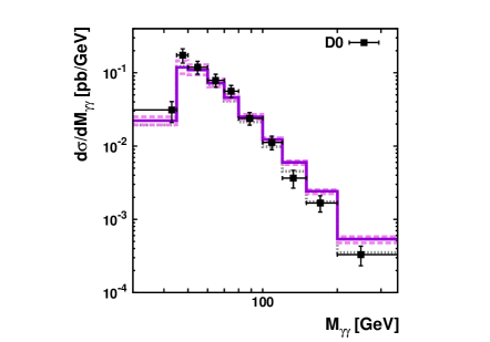
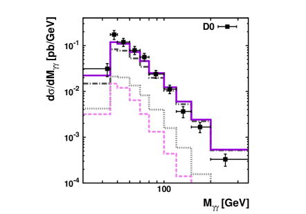
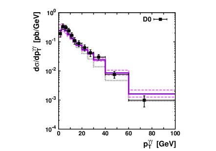
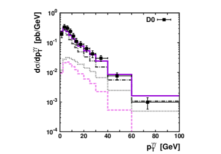
Figure 1: The differential cross section of prompt photon pair production in $p\bar{p}$ collisions at the Tevatron as a function of diphoton invariant mass $M_{\gamma\gamma}$ and transverse momentum $p_{T}^{\gamma\gamma}$. Left panel: the solid histograms correspond to the results obtained with the KMR parton densities at the default scale, and the upper and lower dashed histograms correspond to standard scale variations, as it is described in the text. The dotted histograms represent the NNLL pQCD predictions[13] (as given by resbos program) listed in[3]. Right panel: the different contributions to the diphoton cross sections calculated at the default scale. The dashed, dash-dotted and dotted histograms correspond to the gluon-gluon fusion, quark-antiquark annihilation and quark-gluon scattering subprocesses. The solid histograms represent the sum of these contributions. The experimental data are from D$\emptyset$[3].

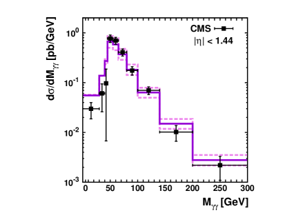
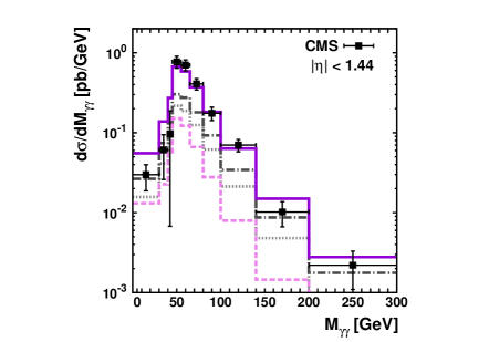
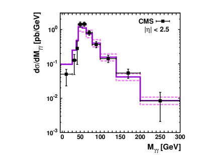
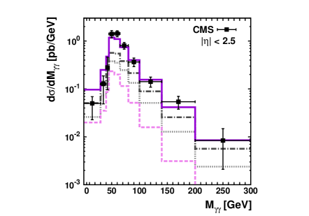
Figure 11: The differential cross section of prompt photon pair production in $pp$ collisions at the LHC as a function of diphoton invariant mass. Left panel: the solid histograms correspond to the results obtained with the KMR parton densities at the default scale, and the upper and lower dashed histograms correspond to standard scale variations, as it is described in the text. Right panel: the different contributions to the diphoton cross sections calculated at the default scale. The dashed, dash-dotted and dotted histograms correspond to the gluon-gluon fusion, quark-antiquark annihilation and quark-gluon scattering subprocesses. The solid histograms represent the sum of these contributions. The experimental data are from CMS[4].

The results of our calculations are shown in Figs. 1 — 10 in comparison with the Tevatron data[1, 2, 3] and in Figs. 11 — 15 in comparison with the LHC data[4, 5]. The solid histograms are obtained by fixing both the factorization and renormalization scales at the default value, whereas the upper and lower dashed histograms correspond to the scale variation as it was described above (in left panels). Also, in Figs. 1 — 6 we plot for comparison the NNLL pQCD predictions[13] (as given by resbos program) listed in[1, 3]. The relative contributions to the diphoton cross sections from quark-antiquark annihilation, quark-gluon scattering and gluon-gluon fusion subprocesses are shown separately by the dash-dotted, dotted and dashed histograms, respectively, in right panels.

We note that different kinematic variables under consideration probe different aspects of the diphoton production mechanism. For instance, the $M_{\gamma\gamma}$ spectrum is particularly sensitive to potential contributions from physics beyond the SM. The $\cos\theta^{*}$ distribution probes the angular momentum of the final state, which should be different for QCD-mediated production as compared, for example, to the decay of a scalar Higgs boson $H\to\gamma\gamma$ (see [13]).

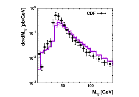
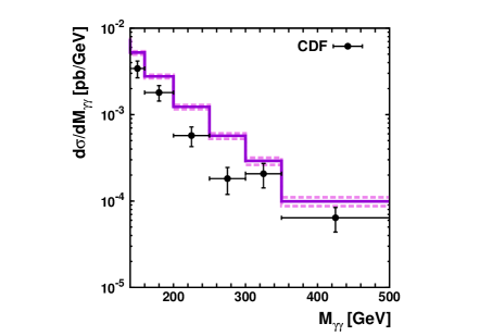
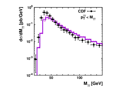
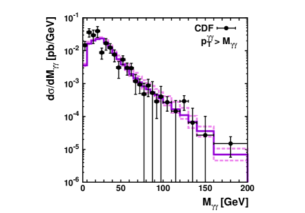
Figure 7: The differential cross section of prompt photon pair production in $p\bar{p}$ collisions at the Tevatron as a function of diphoton invariant mass $M_{\gamma\gamma}$. Two kinematic cases are shown separately: differential cross sections for $M_{\gamma\gamma}>p_{T}^{\gamma\gamma}$ and $M_{\gamma\gamma}<p_{T}^{\gamma\gamma}$. The solid histograms correspond to the results obtained with the KMR parton densities at the default scale, and the upper and lower dashed histograms correspond to standard scale variations, as it is described in the text. The experimental data are from CDF[2].

We find that the $k_{T}$-factorization approach reasonably well describe a full set of experimental data taken at the Tevatron and LHC. Moreover, the shape and absolute normalization of measured cross sections are adequately reproduced within the theoretical and experimental uncertainties. At the Tevatron, there is some discrepancy between recent CDF data[2] and our predictions at very high diphoton invariant masses (see Fig. 7). Note, however, that the small-$x$ approximation used in our consideration is broken at high $M_{\gamma\gamma}$ and the more accurate treatment of, in particular, off-shell quark spin density matrix is needed. This point, of course, is of importance but it is out of our present consideration. From another side, we would like to point out that $k_{T}$-factorization approach provides a better description of all kinematic variables (in comparison with the NLO/NNLL pQCD calculations[12, 13]) at low $M_{\gamma\gamma}$ values, where expected effects connected with the small-$x$ physics becomes important. In the collinear QCD factorization, observed large discrepancy between data and NLO/NNLL pQCD predictions[12, 13] at low $M_{\gamma\gamma}$ attributes to a fragmentation contributions and higher-order QCD corrections to the gluon-gluon fusion subprocess[1, 2, 3, 4, 5]. However, the main part of these corrections are already effectively taken into account in our calculations. It is a radiative QCD corrections described by the ladder-type diagrams which are naturally included into the $k_{T}$-factorization formalism at LO level. At the LHC, our predictions agree well with the CMS data[4] in a whole kinematical range and slightly overestimate the ATLAS data[5] at low values of $\Delta\phi_{\gamma\gamma}$ and high values of $p_{T}^{\gamma\gamma}$. This point, probably, can indicate the inconsistecy of the CMS and ATLAS data and, of course, needs in a further theoretical and experimental investigations. Note also that the NLO pQCD predictions[12] underestimate the measured $\cos\theta^{*}$ distributions at both the Tevatron and LHC energies[2, 3, 4, 5]. This underestimation is more significant for the central rapidity range ($|\eta|<1.44$) at the LHC. Our predictions agree well with the data[2, 3, 4, 5]. It could be important for experimental detection of Higgs boson signal and further investigations of Higgs properties.

Source	$\sigma(p\bar{p}\to\gamma\gamma+X)$ [pb]
$k_{T}$-factorization (KMR)	$29.9^{+7.4}_{-6.1}$ (scales)
NLO pQCD[12] (diphox)	$27.3$ ${}^{+3.0}_{-2.3}$ (scales) $\pm 1.1$ (PDFs)
CMS data[2]	$31.0\pm 1.8$ (stat.) ${}^{+2.0}_{-2.1}$ (syst.) $\pm 1.2$ (lumi.)

Table 2: The total cross section of diphoton production in $pp$ collisions calculated in the kinematical region defined by $|\eta^{\gamma 1}|<1.44$, $|\eta^{\gamma 2}|<1.44$, $p_{T}^{\gamma 1}>23$ GeV and $p_{T}^{\gamma 2}>20$ GeV at $\sqrt{s}=7$ TeV.

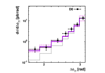
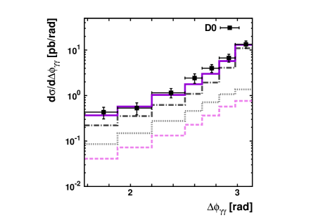
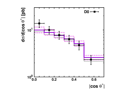
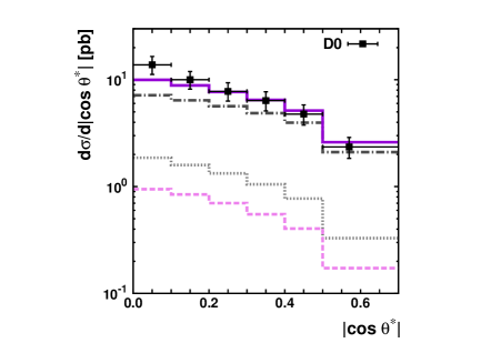
Figure 2: The differential cross section of prompt photon pair production in $p\bar{p}$ collisions at the Tevatron as a function of $\Delta\phi_{\gamma\gamma}$ and $|\cos\theta^{*}|$. Notation of all histograms is the same as in Fig. 2. The experimental data are from D$\emptyset$[3].

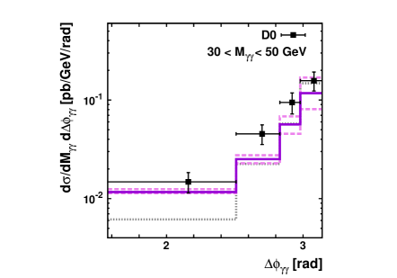
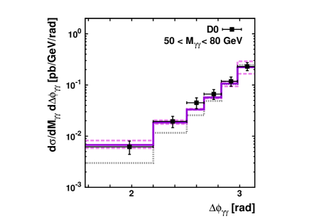
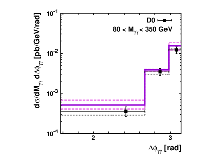
Figure 4: The double differential cross section $d\sigma/dM_{\gamma\gamma}d\Delta\phi_{\gamma\gamma}$ of prompt photon pair production in $p\bar{p}$ collisions at the Tevatron calculated for three subdivisions of $M_{\gamma\gamma}$ range. Notation of all histograms is the same as in Fig. 3. The experimental data are from D$\emptyset$[3].

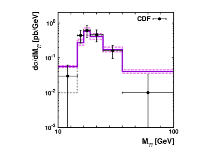
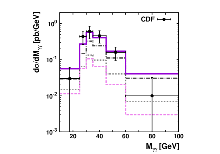
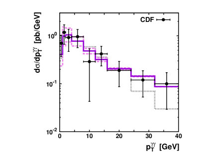
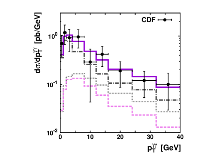
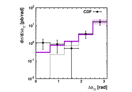
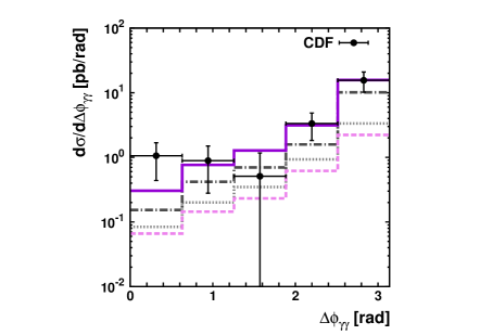
Figure 6: The differential cross section of prompt photon pair production in $p\bar{p}$ collisions at the Tevatron. Notation of all histograms is the same as in Fig. 2. The experimental data are from CDF[1].

As it was expected, the main important properties of the $k_{T}$-factorization approach clearly manifest themselves in the calculated $p_{T}^{\gamma\gamma}$, $z$ and $\Delta\phi_{\gamma\gamma}$ distributions. In the naive LO pQCD approximation, photons produced in $2\to 2$ subprocesses are back-to-back in the transverse plane and are balanced in $p_{T}$ due to momentum conservation. Therefore, these three ditsributions must be simply a delta functions: $d\sigma/dp_{T}^{\gamma\gamma}\sim\delta(p_{T}^{\gamma\gamma})$, $d\sigma/dz\sim\delta(z-1)$ and $d\sigma/d\Delta\phi_{\gamma\gamma}\sim\delta(\Delta\phi_{\gamma\gamma}-\pi)$. When higher-order QCD processes are considered, the presence of additional quarks and/or gluons in the final state allows these distributions to be more spread. In the $k_{T}$-factorization approach, taking into account the non-vanishing initial parton transverse momentum leads to the violation of back-to-back kinematics even at LO approximation. So, despite the fact that one from contributed subprocesses is the $2\to 3$ subprocess (that makes the difference between the $k_{T}$-factorization predictions and ones from the collinear approximation of QCD not well pronounced), obtained perfect description of measured $\Delta\phi_{\gamma\gamma}$ distributions[1, 2, 3, 4, 5] is notable. Specially we point out a reasonable description of the Tevatron and LHC data at low $\Delta\phi_{\gamma\gamma}$ values where the significant underestimation of the data by the NLO/NNLL pQCD calculations[12, 13] was observed (see also Figs. 2, 4 and 6). The important role of such angular correlations for understanding an interaction dynamics is well known[18]. In particular, as it was demonstrated in[33], these correlations strongly depend on the unintegrated parton densities involved in the calculations and can be used as a test to distinguish the different approaches of non-collinear parton evolution. We would like to note also that the scale uncertainties of our calculations are quite small at $\Delta\phi_{\gamma\gamma}\sim 0$ and increases when $\Delta\phi_{\gamma\gamma}\to\pi$. Similar to $\Delta\phi_{\gamma\gamma}$ distributions, the calculated $p_{T}^{\gamma\gamma}$ distributions also directly connected with the unintegrated quark and gluon distributions due to transverse momentum conservation. Perfect overall agreement of our calculations and the data on the $\Delta\phi_{\gamma\gamma}$ and $p_{T}^{\gamma\gamma}$ shows that the KMR prescription for evaluation of unintegrated parton densities reproduces well the transverse momenta of initial quarks and gluons in a probed kinematical region.

Source	$\sigma(p\bar{p}\to\gamma\gamma+X)$ [pb]
$k_{T}$-factorization (KMR)	$59.2^{+14.4}_{-12.1}$ (scales)
NLO pQCD[12] (diphox)	$52.7$ ${}^{+5.8}_{-4.2}$ (scales) $\pm 2.0$ (PDFs)
CMS data[2]	$62.4\pm 3.6$ (stat.) ${}^{+5.3}_{-5.8}$ (syst.) $\pm 2.5$ (lumi.)

Table 3: The total cross section of diphoton production in $pp$ collisions calculated in the kinematical region defined by $|\eta^{\gamma 1}|<2.5$, $|\eta^{\gamma 2}|<2.5$ (except pseudo-rapidity region $1.44<\eta<1.57$ for both photons), $p_{T}^{\gamma 1}>23$ GeV and $p_{T}^{\gamma 2}>20$ GeV at $\sqrt{s}=7$ TeV.

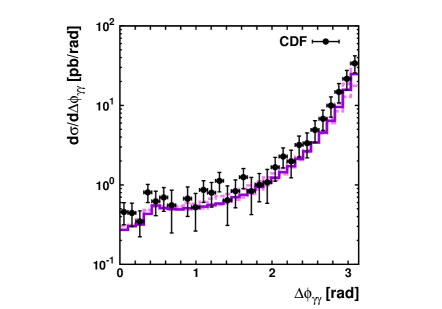
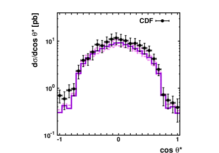
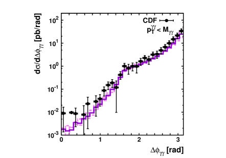
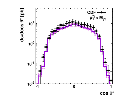
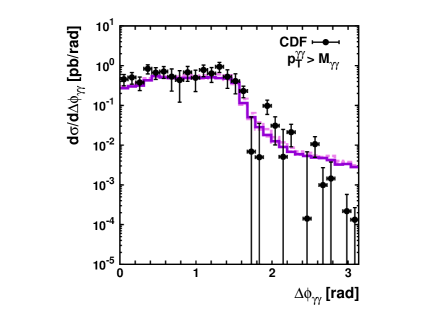
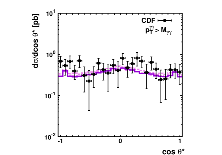
Figure 10: The differential cross section of prompt photon pair production in $p\bar{p}$ collisions at the Tevatron as a function of $\Delta\phi_{\gamma\gamma}$ and $\cos\theta^{*}$. Two kinematic cases are shown separately: differential cross sections for $M_{\gamma\gamma}>p_{T}^{\gamma\gamma}$ and $M_{\gamma\gamma}<p_{T}^{\gamma\gamma}$. Notation of all histograms is the same as in Fig. 7. The experimental data are from CDF[2].

Special interest for the $k_{T}$-factorization phenomenology is connected also with the events with low invariant mass and high transverse momentum of produced photon pair. The CDF collaboration has studied this kinematical region using a special condition $M_{\gamma\gamma}<p_{T}^{\gamma\gamma}$ in their experimental analysis[2]. Within the mentioned above cuts on the transverse momenta of the produced photons, such measurements provide us with an additional test for unintegrated quark and gluon distributions $f_{a}(x,{\mathbf{k}}_{T}^{2},\mu^{2})$ at moderate and high ${\mathbf{k}}_{T}^{2}$ values. The events with back-to-back kinematics are strongly suppressed in this case (see Fig. 10). In contrast with the NLO/NNLL pQCD calculations[12, 13], the $k_{T}$-factorization predictions agree well with the CDF data. An opposite condition (namely, $M_{\gamma\gamma}>p_{T}^{\gamma\gamma}$) corresponds to the selection of events with kinematics similar to the decay of a heavy particle with low transverse momentum into a photon pair, such as, for example, $H\to\gamma\gamma$. Such events are better described[2] by the NLO pQCD calculations[12] than ones with low invariant mass and high transverse momentum. Our predictions agree within the uncertainties with the data[2], but overall agreement is a bit worse.

Concerning a relative contributions to the calculated diphoton production cross sections, we find that quark-antiquark subprocess dominates at both the Tevatron and LHC energies in the probed kinematical regions. The contribution from quark-gluon scattering is similar to gluon-gluon fusion one at low diphoton invariant masses and overshoot gluon-gluon fusion contribution at high $M_{\gamma\gamma}$ values. As it was expected[4, 5], the role of both these subprocesses increases significantly at the LHC energies. We note also that the contribution from $q\bar{q}\to\gamma\gamma g$ subprocess, which is order of ${\cal O}(\alpha_{s}\alpha^{2})$, is already taken into account in our calculations. To be precise, this contribution is effectively included to the quark-antiquark annihilation one due to the initial state gluon radiation (see also[18]). Of course, it is in a clear contrast with the collinear QCD factorization where these contributions should be calculated separately.

The predicted total cross sections for the Tevatron conditions are listed in Table 1 and for LHC conditions are listed in Tables 2 and 3, respectively. Our results are slightly below the Tevatron data and NLO/NNLL pQCD predictions[12, 13] but agree with them within the theoretical and experimental uncertainties. However, at the LHC energy, our predictions overshoot the NLO pQCD ones[12] and are more close to the data. It could be connected with the small-$x$ effects which becomes more important for the LHC conditions.

In conclusion, we would like to stress a number of important achievements demonstrated by the $k_{T}$-factorization QCD approach. As a general feature, the $k_{T}$-factorization predictions are found to be perfectly compatible with the available data, in particular, on the production of prompt photons, Drell-Yan lepton pairs, heavy quarks as well as various quarkonium states at modern colliders[20, 21, 22, 23, 24, 25, 33, 35, 36]. The $k_{T}$-factorization approach succeeds in describing the polarization phenomena observed in $ep$ and $pp$ interactions (see, for example,[35, 36] and references therein). The latter is essentially related to the initial gluon off-shellness, which dominates the gluon polarization properties and has a considerable impact on the kinematics. So, we believe that the $k_{T}$-factorization formalism holds a possible key to understanding the production dynamics at high energies.

4 Conclusions

We have investigated the isolated prompt photon pair production in $p\bar{p}$ and $pp$ collisions at the Tevatron and LHC energies within the framework of the $k_{T}$-factorization QCD approach. Our consideration is based on the quark-antiquark annihilation, quark-gluon scattering and gluon-gluon fusion subprocesses, where the non-zero transverse momenta of incoming partons are taken into account. The unintegrated parton densities in a proton are determined using the Kimber-Martin-Ryskin prescription. We obtained a reasonable well agreement between our predictions and recent data taken by the D$\emptyset$, CDF, CMS and ATLAS collaborations. The achieved description of the data in several kinematical regions (in particular, at low azimuthal angle distance between produced photons) is better as compared to the one obtained in the framework of collinear QCD factorization (with NLO or even NNLL accuracy). Also, we describe reasonably well the Tevatron and LHC data on the $\cos\theta^{*}$ distributions of the diphoton production. Such quantities (underestimated by the NLO pQCD calculations) probe the angular momentum of the final state and different for QCD-mediated production as compared to the decay of a scalar Higgs boson. It could be important for experimental detection of Higgs and further theoretical and experimental investigations in this field. We find that the scale uncertainties of our calculations are quite small at $\Delta\phi_{\gamma\gamma}\sim 0$, although they are exceed, of course, the uncertainties of NLO/NNLL pQCD calculations in general. Moreover, the problem of estimation of our theoretical uncertainties (connected in part with the non-collinear parton evolution scheme) is still open and further theoretical attempts (in order to investigate the unintegrated quark distributions more detail) are necessary to reduce this uncertainty. It is important for further studies of small-$x$ physics at hadron colliders, and, in particular, for searches of effects of new physics beyond the SM at the LHC.

5 Acknowledgments

The author would like to thank N.P. Zotov, S.P. Baranov and H. Jung for their encouraging interest and helpful discussions. Author is also grateful to DESY Directorate for the support in the framework of Moscow — DESY project on Monte-Carlo implementation for HERA — LHC. This research was supported in part by the FASI of Russian Federation (grant NS-3920.2012.2), RFBR grants 11-02-01454-a and 12-02-31030, grant of president of Russian Federation (MK-3977.2011.2) and the grant of Ministry of education and sciences of Russia (agreement 8412).

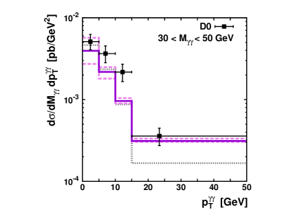
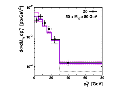
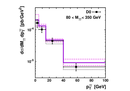
Figure 3: The double differential cross section $d\sigma/dM_{\gamma\gamma}dp_{T}^{\gamma\gamma}$ of prompt photon pair production in $p\bar{p}$ collisions at the Tevatron calculated for three subdivisions of $M_{\gamma\gamma}$ range. The solid histograms correspond to the results obtained with the KMR parton densities at the default scale, and the upper and lower dashed histograms correspond to standard scale variations, as it is described in the text. The dotted histograms represent the NNLL pQCD predictions[13] (as given by resbos program) listed in[3]. The experimental data are from D$\emptyset$[3].

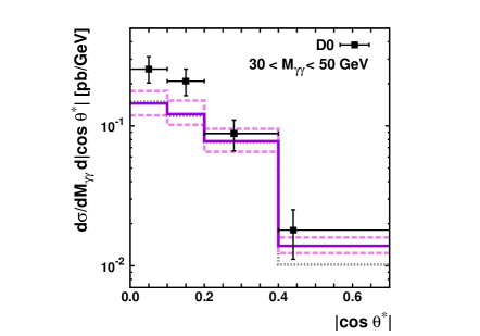
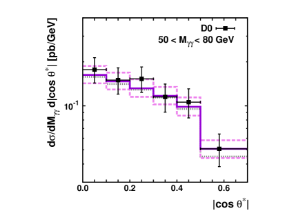
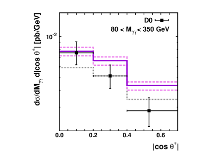
Figure 5: The double differential cross section $d\sigma/dM_{\gamma\gamma}d|\cos\theta^{*}|$ of prompt photon pair production in $p\bar{p}$ collisions at the Tevatron calculated for three subdivisions of $M_{\gamma\gamma}$ range. Notation of all histograms is the same as in Fig. 3. The experimental data are from D$\emptyset$[3].

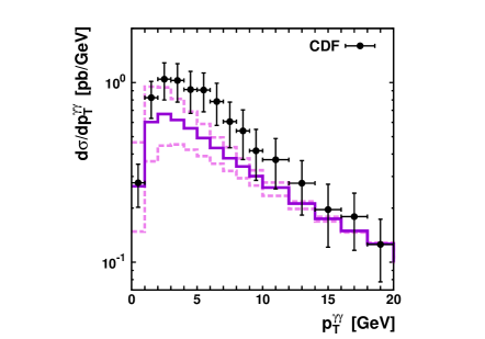
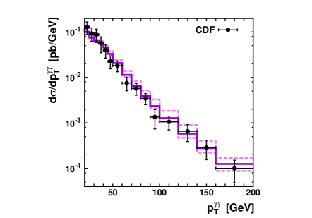
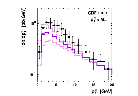
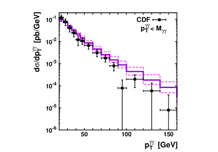
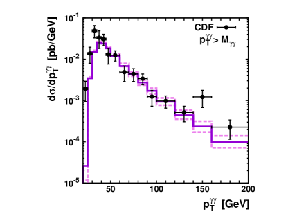
Figure 8: The differential cross section of prompt photon pair production in $p\bar{p}$ collisions at the Tevatron as a function of diphoton transverse momentum $p_{T}^{\gamma\gamma}$. Two kinematic cases are shown separately: differential cross sections for $M_{\gamma\gamma}>p_{T}^{\gamma\gamma}$ and $M_{\gamma\gamma}<p_{T}^{\gamma\gamma}$. Notation of all histograms is the same as in Fig. 7. The experimental data are from CDF[2].

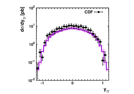
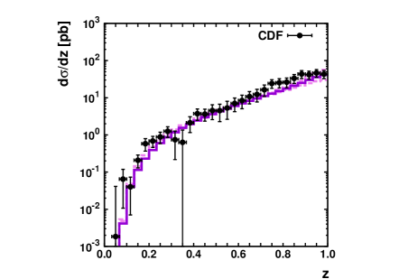
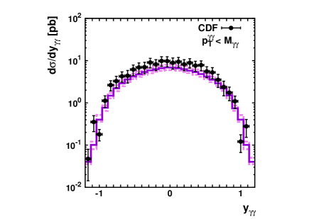
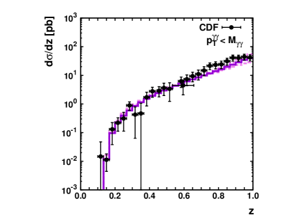
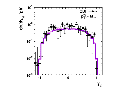
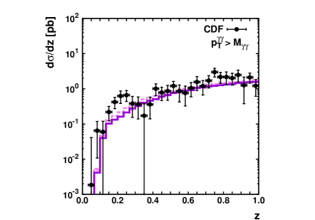
Figure 9: The differential cross section of prompt photon pair production in $p\bar{p}$ collisions at the Tevatron as a function of diphoton rapidity $y_{\gamma\gamma}$ and variable $z=p_{T}^{\gamma 2}/p_{T}^{\gamma 1}$. Two kinematic cases are shown separately: differential cross sections for $M_{\gamma\gamma}>p_{T}^{\gamma\gamma}$ and $M_{\gamma\gamma}<p_{T}^{\gamma\gamma}$. Notation of all histograms is the same as in Fig. 7. The experimental data are from CDF[2].

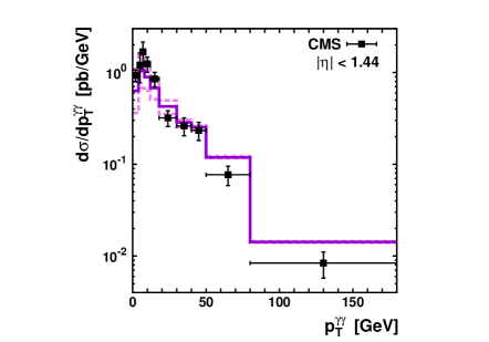
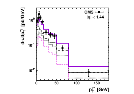
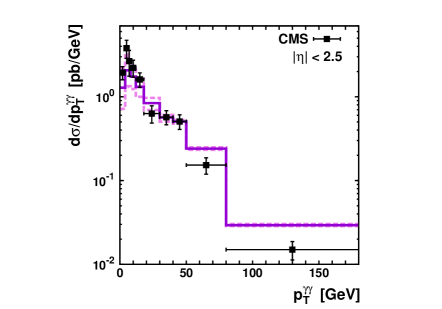
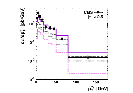
Figure 12: The differential cross section of prompt photon pair production in $pp$ collisions at the LHC as a function of diphoton transverse momentum. Notation of all histograms is the same as in Fig. 11. The experimental data are from CMS[4].

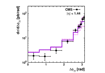
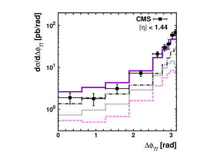
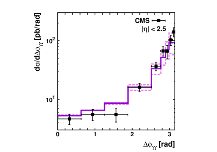
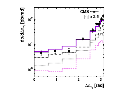
Figure 13: The differential cross section of prompt photon pair production in $pp$ collisions at the LHC as a function of $\Delta\phi_{\gamma\gamma}$. Notation of all histograms is the same as in Fig. 11. The experimental data are from CMS[4].

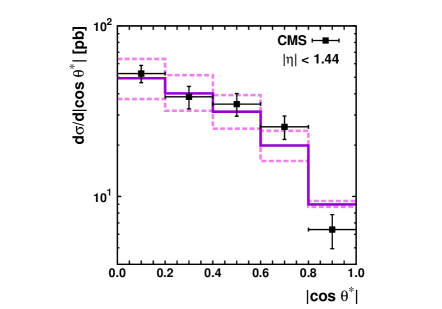
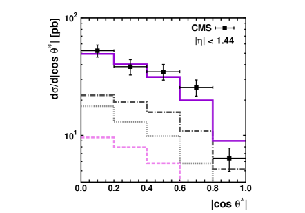
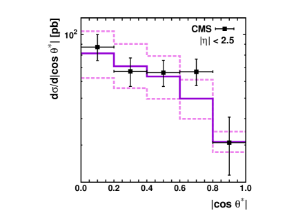
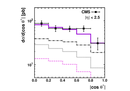
Figure 14: The differential cross section of prompt photon pair production in $pp$ collisions at the LHC as a function of $|\cos\theta^{*}|$. Notation of all histograms is the same as in Fig. 11. The experimental data are from CMS[4].

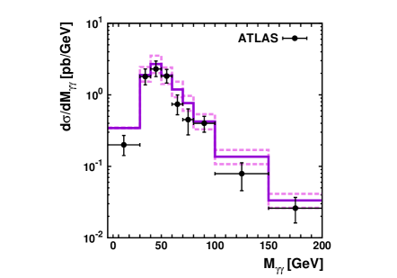
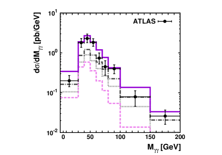
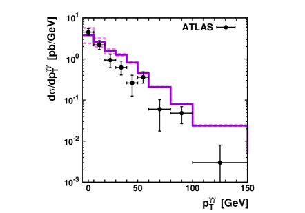
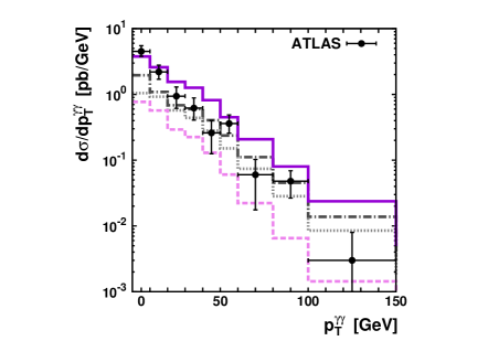
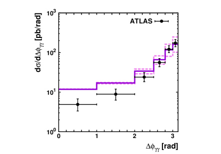
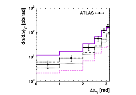
Figure 15: The differential cross section of prompt photon pair production in $pp$ collisions at the LHC. Notation of all histograms is the same as in Fig. 11. The experimental data are from ATLAS[5].

References

- [1] D. Acosta et al. (CDF Collaboration), Phys. Rev. Lett. 95, 022003 (2005).
- [2] T. Aaltonen et al. (CDF Collaboration), Phys. Rev. D 84, 052006 (2011).
- [3] V. Abazov et al. (D Collaboration), Phys. Lett. B 690, 108 (2010).
- [4] CMS Collaboration, JHEP 01, 133 (2012).
- [5] ATLAS Collaboration, Phys. Rev. D 85, 012003 (2012).
- [6] S. Mrenna and J. Willis, Phys. Rev. D 63, 015006 (2001).
- [7] G.F. Giudice and R. Rattazzi, Phys. Rep. 322, 419 (1999).
- [8] T. Appelquist, H. Cheng, and B. Dobrescu, Phys. Rev. D 64, 035002 (2001).
- [9] ATLAS Collaboration, Phys. Rev. Lett. 106, 121803 (2011).
- [10] L. Randall and R. Sundrum, Phys. Rev. Lett. 83, 3370 (1999).
- [11] K. Koller, T.F. Walsh, and P.M. Zerwas, Z. Phys. C 2, 197 (1979).
-
[12]
T. Binoth, J.P. Guillet, E. Pilon, and M. Werlen, Eur. Phys. J. C 16, 311 (2000);
T. Binoth, J.P. Guillet, E. Pilon, and M. Werlen, Phys. Rev. D 63, 114016 (2001). - [13] C. Balazs, E.L. Berger, P. Nadolsky and C.-P. Yuan, Phys. Rev. D 76, 013009 (2007).
-
[14]
L.V. Gribov, E.M. Levin, and M.G. Ryskin, Phys. Rep. 100, 1 (1983);
E.M. Levin, M.G. Ryskin, Yu.M. Shabelsky and A.G. Shuvaev, Sov. J. Nucl. Phys. 53, 657 (1991). -
[15]
S. Catani, M. Ciafoloni and F. Hautmann, Nucl. Phys. B 366, 135 (1991);
J.C. Collins and R.K. Ellis, Nucl. Phys. B 360, 3 (1991). -
[16]
E.A. Kuraev, L.N. Lipatov and V.S. Fadin, Sov. Phys. JETP 44, 443 (1976);
E.A. Kuraev, L.N. Lipatov and V.S. Fadin, Sov. Phys. JETP 45, 199 (1977);
I.I. Balitsky and L.N. Lipatov, Sov. J. Nucl. Phys. 28, 822 (1978). -
[17]
M. Ciafaloni, Nucl. Phys. B 296, 49 (1988);
S. Catani, F. Fiorani and G. Marchesini, Phys. Lett. B 234, 339 (1990);
S. Catani, F. Fiorani and G. Marchesini, Nucl. Phys. B 336, 18 (1990);
G. Marchesini, Nucl. Phys. B 445, 49 (1995). -
[18]
B. Andersson et al. (Small- Collaboration), Eur. Phys. J. C 25, 77 (2002);
J. Andersen et al. (Small- Collaboration), Eur. Phys. J. C 35, 67 (2004);
J. Andersen et al. (Small- Collaboration), Eur. Phys. J. C 48, 53 (2006). - [19] A. Gawron and J. Kwiecinski, Phys. Rev. D 70, 014003 (2004).
-
[20]
S.P. Baranov, A.V. Lipatov and N.P. Zotov, Phys. Rev. D 81, 094034 (2010);
A.V. Lipatov and N.P. Zotov, Phys. Rev. D 81, 094027 (2010); Phys. Rev. D 72, 054002 (2005). - [21] A.V. Lipatov and N.P. Zotov, J. Phys. G 34, 219 (2007).
- [22] S.P. Baranov, A.V. Lipatov and N.P. Zotov, Phys. Rev. D 77, 074024 (2008).
- [23] A.V. Lipatov, M.A. Malyshev and N.P. Zotov, Phys. Lett. B 699, 93 (2011).
- [24] A.V. Lipatov, M.A. Malyshev and N.P. Zotov, JHEP 1112, 117 (2011).
- [25] A.V. Lipatov, M.A. Malyshev and N.P. Zotov, JHEP 1205, 104 (2012).
-
[26]
M.A. Kimber, A.D. Martin and M.G. Ryskin, Phys. Rev. D 63, 114027 (2001);
G. Watt, A.D. Martin and M.G. Ryskin, Eur. Phys. J. C 31, 73 (2003). -
[27]
R.E. Prange, Phys. Rev. 110, 240 (1958);
S.P. Baranov, Phys. Atom. Nucl. 60, 1322 (1997). - [28] J.A.M. Vermaseren, ”Symbolic Manipulation with FORM”, published by Computer Algebra Nederland, Kruislaan 413, 1098, SJ Amsterdaam, 1991; ISBN 90-74116-01-9.
- [29] E.L. Berger, E. Braaten, and R.D. Field, Nucl. Phys. B 239, 52 (1984).
- [30] A.D. Martin, W.J. Stirling, R.S. Thorne and G. Watt, Eur. Phys. J. C 63, 189 (2009).
- [31] M. Fontannaz, J.Ph. Guillet and G. Heinrich, Eur. Phys. J. C 21, 303 (2001).
- [32] G.P. Lepage, J. Comput. Phys. 27, 192 (1978).
- [33] S.P. Baranov, A.V. Lipatov and N.P. Zotov, Yad. Fiz. 67, 856 (2004).
- [34] V.A. Saleev, Phys. Rev. D 80, 114016 (2009).
-
[35]
S.P. Baranov, A.V. Lipatov and N.P. Zotov, Phys. Rev. D 85, 014034 (2012);
S.P. Baranov, A.V. Lipatov and N.P. Zotov, Eur. Phys. J. C 71, 1631 (2011). - [36] S.P. Baranov and N.P. Zotov, JETP Lett. 88, 711 (2008).