The $\langle VVA\rangle$ correlator at three loops in perturbative QCD

Abstract

It is known that the correlator of one axial and two vector currents, that receives leading contributions through one-loop fermion triangle diagrams, is not modified by QCD radiative corrections at two loops. It was suggested that this non-renormalization of the $\langle VVA\rangle$ correlator persists in higher orders in perturbative QCD as well. To check this assertion, we compute the three-loop QCD corrections to the $\langle VAA\rangle$ correlator using the technique of asymptotic expansions. We find that these corrections do not vanish and that they are proportional to the QCD $\beta$-function.

1 Introduction

The correlator of two vector currents and one axial current is an interesting object. Early studies of this correlator were important for developing an understanding that, in spite of naive equations of motion, the axial current is anomalous and that the perturbative part of the anomaly can be computed exactly from the one-loop triangle diagram [1]. The anomaly corresponds to just one term in the decomposition of the correlator into independent Lorentz structures, and the non-renormalization of the anomaly by higher-order QCD corrections does not say if other terms share the same property. In fact, since the discovery of the non-renormalization of the anomaly, it was generally believed that coefficients of other Lorentz structures change in higher orders of perturbation theory. This belief was challenged in Ref. [2], where it was pointed out that in the kinematic limit where momentum of one of the vector currents is vanishingly small, another non-renormalization theorem is valid. Indeed, in that limit just two independent form factors are needed to fully describe the $\langle VVA\rangle$ correlator. One of these form factors is the axial anomaly and, therefore, it is not renormalized. It was shown in Ref. [2] that due to helicity conservation in massless QCD, the two form factors are in fact proportional to each other, and so the non-renormalization of one of them implies the non-renormalization of the other. Therefore, we come to the conclusion that the entire $\langle VVA\rangle$ correlator is not renormalized in that limit.

This result initiated new studies of the $\langle VVA\rangle$ correlator, which led to a number of surprising findings. First, in Ref. [3] it was pointed out that additional non-renormalization theorems for form factors of the $\langle VVA\rangle$ correlator exist even in the case of the most general kinematics. Later, in Ref. [4] an explicit calculation of the two-loop ${\cal O}(\alpha_{s})$ contribution to the correlator was reported. The result turned out to be extremely simple: it was found that the ${\cal O}(\alpha_{s})$ correction to the correlator vanishes identically in the most general kinematics if a consistent definition of the axial current is employed. This unusual feature of radiative corrections prompted the authors of Ref. [4] to speculate that their result might be an early indication of the non-renormalization of the entire $\langle VVA\rangle$ correlator in perturbative QCD with massless quarks to all orders in the strong coupling constant.

The goal of this Letter is to show that this speculation is not correct and that radiative corrections to the $\langle VVA\rangle$ correlator appear at the three-loop order in perturbative QCD. These three-loop corrections are, however, peculiar in that they are explicitly proportional to the QCD $\beta$-function and vanish in the conformal limit of QCD. This is a natural result. In fact, it was pointed long ago in Ref. [5] that the exact $\langle VVA\rangle$ correlator in a conformally-invariant theory is given by the one-loop expression and no contributions at higher-loops are allowed. This happens because conformal symmetry restricts the functional form of the three-point function up to a possible multiplicative factor which, however, is fixed by the requirement that the non-renormalization of the anomaly works out correctly. It is easy to realize that through two loops in perturbative QCD, no diagrams that cause violation of the conformal symmetry contribute to $\langle VVA\rangle$ correlator, while at three loops diagrams that correspond to the running of the coupling constant explicitly appear. This allows us to understand why no corrections to $\langle VVA\rangle$ correlator were found in Ref. [4], why such corrections appear at the three-loop order, and why they are proportional to the QCD $\beta$-function.

The remainder of this Letter is organized as follows. In the next Section we define the $\langle VVA\rangle$ correlator and discuss its decomposition in terms of invariant form factors. In Section 3 we explain how three-loop contributions to the correlator can be computed. In Section 4 we present the results of the calculation. We conclude in Section 5.

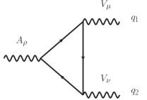
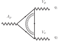
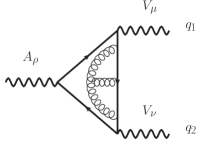
Figure 1: Sample diagrams that contribute to $\langle VVA\rangle$ correlator at one, two and three-loops. The momenta $q_{1,2}$ are outgoing.

2 Definitions

We consider the correlator of two vector currents $V_{\mu}$ and one axial current $A_{\mu}$

$${\cal W}_{\mu\nu\rho}(q_{1},q_{2})=-\int d^{4}x_{1}d^{4}x_{2}\,e^{i(q_{1}\cdot x_{1}+q_{2}\cdot x_{2})}\,\langle\,0\,|\,\mbox{T}\{V_{\mu}(x_{1})V_{\nu}(x_{2})A_{\rho}(0)\}\,|\,0\,\rangle.$$ (1)

The currents are flavor-diagonal. They read

$$V_{\mu}\,=\,{\overline{\psi}}\gamma_{\mu}\,\psi\quad,\quad A_{\mu}\,=\,{\overline{\psi}}\gamma_{\mu}\gamma_{5}\,\psi\,,$$ (2)

where $\psi$ are fermion fields charged under the $SU(N_{c})$ color group.

The $\langle VVA\rangle$ correlator in Eq.(1) can be expressed in terms of independent Lorentz structures and invariant form factors [3]. A suitable parameterization reads

$$\begin{split}{\cal W}_{\mu\nu\rho}(q_{1},q_{2})&=w_{L}(q_{1}^{2},q_{2}^{2},q^{2})t^{(1)}_{\mu\nu\rho}+w_{T}^{(+)}(q_{1}^{2},q_{2}^{2},q^{2})t^{(+)}_{\mu\nu\rho}\\ &+w_{T}^{(-)}(q_{1}^{2},q_{2}^{2},q^{2})t^{(-)}_{\mu\nu\rho}+\tilde{w}_{T}^{(-)}(q_{1}^{2},q_{2}^{2},q^{2}){\tilde{t}}^{(-)}_{\mu\nu\rho}\,,\end{split}$$ (3)

where, following Ref. [3], we introduced four independent tensor structures

$$\begin{split}&t^{(1)}_{\mu\nu\rho}=-q_{\rho}\epsilon_{\mu\nu\alpha\beta}q_{1}^{\alpha}q_{2}^{\beta}\,,\\ &t^{(+)}_{\mu\nu\rho}=q_{1\nu}\epsilon_{\mu\rho\alpha\beta}q_{1}^{\alpha}q_{2}^{\beta}-q_{2\mu}\epsilon_{\nu\rho\alpha\beta}q_{1}^{\alpha}q_{2}^{\beta}-q_{1}\cdot q_{2}\epsilon_{\mu\nu\rho\alpha}\kappa^{\alpha}-2\frac{q_{1}\cdot q_{2}}{q^{2}}\epsilon_{\mu\nu\alpha\beta}q_{1}^{\alpha}q_{2}^{\beta}q_{\rho}\,,\\ &t^{(-)}_{\mu\nu\rho}=\epsilon_{\mu\nu\alpha\beta}q_{1}^{\alpha}q_{2}^{\beta}\kappa_{\rho}-\frac{\kappa\cdot q}{q^{2}}\epsilon_{\mu\nu\alpha\beta}q_{1}^{\alpha}q_{2}^{\beta}q_{\rho}\,,\\ &{\tilde{t}}^{(-)}_{\mu\nu\rho}=q_{1\nu}\epsilon_{\mu\rho\alpha\beta}q_{1}^{\alpha}q_{2}^{\beta}+q_{2\mu}\epsilon_{\nu\rho\alpha\beta}q_{1}^{\alpha}q_{2}^{\beta}-q_{1}\cdot q_{2}\epsilon_{\mu\nu\rho\alpha}q^{\alpha}\,,\end{split}$$ (4)

and momenta $q=q_{1}+q_{2},\;\kappa=q_{1}-q_{2}$. From momentum conservation, $q$ is the incoming momentum carried by the axial current. We note that all tensor structures are transversal with respect to the momenta of the vector currents

$$q_{1}^{\mu}t_{\mu\nu\rho}=0,\;\;\;q_{2}^{\nu}t_{\mu\nu\rho}=0\,,$$ (5)

where $t_{\mu\nu\rho}$ is a generic notation for $t^{(1)}_{\mu\nu\rho},t^{(\pm)}_{\mu\nu\rho}$ and ${\tilde{t}}^{(+)}_{\mu\nu\rho}$. On the other hand, these tensor structures have different transversality properties with respect to the momentum $q$ of the axial current,

$$q^{\rho}t^{(1)}_{\mu\nu\rho}=-q^{2}\epsilon_{\mu\nu\alpha\beta}q_{1}^{\alpha}q_{2}^{\beta}\,,\;\;\;\;q^{\rho}t^{(\pm)}_{\mu\nu\rho}=0\,,\;\;\;\;q^{\rho}{\tilde{t}}^{(-)}_{\mu\nu\rho}=0\,.$$ (6)

Therefore, the parameterization in Eq.(3) is consistent with the conservation of the vector current and with the fact that the conservation of the axial current is violated by triangle loop diagrams. We will refer to $w_{L}$ as the longitudinal form factor and to $w_{T}^{(\pm)}$ and ${\tilde{w}}_{T}^{(-)}$ as the transversal form factors.

We now discuss what is known about these form factors. In general, they are functions of three independent kinematic variables, $q_{1}^{2},q_{2}^{2}$ and $q^{2}=(q_{1}+q_{2})^{2}$. Since the divergence of the axial current is fixed by the anomaly equation

$$\partial_{\mu}A^{\mu}=\frac{N_{c}}{16\pi^{2}}\epsilon_{\mu\nu\rho\sigma}F^{\mu\nu}F^{\rho\sigma}\,,$$ (7)

to all orders in perturbation theory, the longitudinal form factor $w_{L}$ is completely defined. Indeed, the anomaly equation implies

$$q^{\rho}{\cal W}_{\mu\nu\rho}=-w_{L}(q_{1}^{2},q_{2}^{2},q^{2})q^{2}\epsilon_{\mu\nu\alpha\beta}q_{1}^{\alpha}q_{2}^{\beta}=-\frac{iN_{c}}{2\pi^{2}}\epsilon_{\alpha\beta\mu\nu}q_{1}^{\alpha}q_{2}^{\beta}\,.$$ (8)

We solve this equation for $w_{L}$ to find

$$w_{L}(q_{1}^{2},q_{2}^{2},q^{2})=\frac{i\,N_{c}}{2\pi^{2}q^{2}}\,.$$ (9)

While the longitudinal form factor can be fully determined from the anomaly equation, the transversal form factors can not. However, as it was shown in Refs. [2, 3], some combinations of transversal form factors are uniquely fixed by the chiral symmetry in perturbative QCD with massless flavors. The following relations are valid [3],

$$\begin{split}&\left[w_{T}^{(+)}+w_{T}^{(-)}\right](q_{1}^{2},q_{2}^{2},q^{2})-\left[w_{T}^{(+)}+w_{T}^{(-)}\right](q^{2},q_{2}^{2},q_{1}^{2})=0\,,\\ &\left[{\tilde{w}}_{T}^{(-)}+w_{T}^{(-)}\right](q_{1}^{2},q_{2}^{2},q^{2})+\left[{\tilde{w}}_{T}^{(-)}+w_{T}^{(-)}\right](q^{2},q_{2}^{2},q_{1}^{2})=0\,,\\ &\left[w_{T}^{(+)}+{\tilde{w}}_{T}^{(-)}\right](q_{1}^{2},q_{2}^{2},q^{2})+\left[w_{T}^{(+)}+{\tilde{w}}_{T}^{(-)}\right](q^{2},q_{2}^{2},q_{1}^{2})-w_{L}(q^{2},q_{2}^{2},q_{1}^{2})\\ &=-\left[2\frac{q_{2}\cdot q}{q_{1}^{2}}w_{T}^{(+)}(q^{2},q_{2}^{2},q_{1}^{2})-2\frac{q_{1}\cdot q_{2}}{q_{1}^{2}}w_{T}^{(-)}(q^{2},q_{2}^{2},q_{1}^{2})\right]\,.\end{split}$$ (10)

In perturbation theory, the correlator ${\cal W}_{\mu\nu\rho}$ receives contributions starting at one-loop order, see Fig. 1. The correlator was computed through two loops in Ref. [4] for arbitrary momenta $q_{1}$ and $q_{2}$. The results of that calculation showed that, with the proper definition of the axial current, the two-loop corrections to the full correlator vanish. We pointed out a possible reason for that in Section 1, where we noted that it is natural to expect that these results will be violated starting from three loops. In the next Section we discuss how to set up a calculation to check this explicitly.

3 The three-loop calculation

We are interested in computing the ${\cal W}_{\mu\nu\rho}$ correlator to three loops in perturbative QCD, for arbitrary $q_{1}$ and $q_{2}$. Sample diagrams are shown in Fig. 1. We note that the one-loop contribution is described by 2 diagrams, the two-loop contribution by 12 diagrams and the three-loop contribution by 182 diagrams. It goes without saying that, at present, no computational technology exists that can be used to calculate three-loop three-point functions with three external off-shell legs. To circumvent this problem, we consider a hierarchy of incoming momenta, $q_{2}\ll q_{1}$, and construct a systematic expansion of the three-loop diagrams in the ratio $q_{2}/q_{1}$. It is intuitively clear that, upon such an expansion, a three-point function is mapped onto a set of two-point functions and its derivatives evaluated either for small $k\sim q_{2}$ or large $k\sim q_{1}$ loop momenta. Such an expansion is constructed most efficiently by using standard techniques of the large momentum expansion [8]. In the current application, we use this procedure as automated in the computer programs q2e and exp [9, 10]. Once the three-loop three-point functions are mapped onto the three-loop two-point functions by the large momentum expansion procedure, we use the program MINCER [12] to compute them. Finally, we note that all diagrams that contribute to the correlator are generated with Qgraf [7].

As a technical remark, we note that treatment of tensor integrals that appear in this computation requires some care. At one loop, MINCER routines can deal with tensor integrals of arbitrary rank, contracted with arbitrary external momenta. Unfortunately, at higher loops MINCER can only be used to compute two-point scalar integrals that depend on a single external momentum. However, since we arrive at relevant two-point functions by expanding three-point functions in $q_{2}/q_{1}$, we need to compute more complicated tensor integrals. To give an example, consider an integral

$$\int\prod\limits_{i=1}^{3}\frac{{\rm d}^{d}k_{i}}{(2\pi)^{d}}\frac{(k_{1}\cdot q_{2})^{a_{1}}(k_{2}\cdot q_{2})^{a_{2}}..}{k_{1}^{2}k_{2}^{2}...(k_{1}-q_{1})^{2}..(k_{2}-q_{1})^{2}..},$$ (11)

where the two-point function itself depends on momentum $q_{1}$ but the numerator contains scalar products of loop momenta $k_{i}$ with another external momentum $q_{2}$. This is a typical situation for us to face, and it can not be handled by MINCER. To deal with the integrals of the type shown in Eq.(11), we write $q_{2}^{\mu}=(q_{2}\cdot q_{1})/q_{1}^{2}q_{1}^{\mu}+q_{2,\perp}^{\mu},$ where $q_{2,\perp}\cdot q_{1}=0$, and note that the final result can not depend on the direction of $q_{2,\perp}$. We make use of this observation by averaging over directions of $q_{2,\perp}$ in Eq.(11). Such averages are constructed from the metric tensor $g^{\mu\nu}-q_{1}^{\mu}q_{1}^{\mu}/q_{1}^{2}$ which only contains vector $q_{1}$ and, therefore, leads to scalar products of four-momenta that can be treated by MINCER.

Computational procedures described above rely heavily on the use of dimensional regularization. This leads to a subtlety since, as it is well known, continuation of the Dirac matrix $\gamma_{5}$ to $d$ dimensions requires care and a proper way to do so is crucial for the correct computation of the $\langle VVA\rangle$ correlator. We use the definition of the axial current developed in Ref. [6] which, on one hand, is self-consistent and, on the other hand, does not introduce unnecessary difficulties into already complicated multi-loop computation. Thus, we define the axial current in the following way [6],

$$A_{\rho}\equiv\frac{i}{6}\epsilon_{\rho\alpha^{\prime}\beta^{\prime}\lambda^{\prime}}{\bar{\psi}}\Gamma^{[\alpha^{\prime}\beta^{\prime}\lambda^{\prime}]}\psi,\quad\text{with}\,\,\,\epsilon_{0123}=1=-\epsilon^{0123}\,,$$ (12)

where $\Gamma^{\alpha\beta\lambda}=\gamma^{\alpha}\gamma^{\beta}\gamma^{\lambda}$ and square brackets indicate the anti-symmetrization of the Lorentz indices,

$$\Gamma^{[\alpha\beta\lambda^{\prime}]}=\frac{1}{6}\left(\gamma^{\alpha}\gamma^{\beta}\gamma^{\lambda}-\gamma^{\alpha}\gamma^{\lambda}\gamma^{\beta}+\dots\right)\,.$$ (13)

With this definition, the axial current needs renormalization. We write $A_{\rho}=Z_{A}A_{\rho}^{\rm bare}$ and note that the renormalization constant $Z_{A}$ was worked out in Ref. [6]. There, in addition to the $\overline{\rm MS}$ renormalization constant, a finite piece is added that ensures that the non-singlet current has no anomalous dimension and the anomaly equation (7) is satisfied. The full renormalization constant reads at two loops

$$\begin{split}Z_{A}=&\left(1+\frac{2a_{s}^{2}C_{F}}{\epsilon}\beta_{0}\right)\times\left(1-4C_{F}a_{s}+C_{F}a_{s}^{2}\left(22\,C_{F}-\frac{107}{9}\,C_{A}+\frac{2}{9}\,n_{f}\right)\right)\,,\end{split}$$ (14)

where $a_{s}=g^{2}(\mu)/(16\pi^{2})$ is the $\overline{\rm MS}$ QCD coupling constant defined at the scale $\mu$ and $\beta_{0}=11/3C_{A}-2/3n_{f}$ is the one-loop QCD $\beta$-function. Also, $n_{f}$ is the number of (massless) quark flavors and $C_{F}=(N_{c}^{2}-1)/(2N_{c})$, $C_{A}=N_{c}$ are the Casimir operators of the ${\rm SU}(N)$ group in fundamental and adjoint representations, respectively. In QCD, we use $N=3$.

We now return to the definition of the axial current in Eq. (12) and observe that it contains the Levi-Civita tensor $\epsilon_{\mu\nu\alpha\rho}$, which is a four-dimensional object whose continuation to $d$ dimensions is not possible. To address this issue, we first compute an auxiliary tensor correlator ${\cal T}_{\alpha\beta\lambda,\mu\nu}$ which does not contain the Levi-Civita tensor and which is finite at $d=4$. We then obtain the required correlator by contracting ${\cal T}_{\alpha\beta\lambda,\mu\nu}$ with the Levi-Civita tensor

$${\cal W}_{\mu\nu\rho}=\frac{i}{6}\epsilon_{\rho\alpha\beta\lambda}{\cal T}_{\alpha\beta\lambda,\mu\nu}\,.$$ (15)

This can be easily done because all entries on the right hand side of Eq.(15) are well-defined in four dimensions.

To define the auxiliary tensor ${\cal T}_{\alpha\beta\lambda,\mu\nu}$, we imagine that the correlator ${\cal W}_{\mu\nu\rho}$ is contracted with $\epsilon_{\alpha\beta\lambda\rho}$

$${\cal T}_{\alpha\beta\lambda,\mu\nu}(q_{1},q_{2})\equiv\frac{1}{i}\epsilon_{\alpha\beta\lambda\rho}{\cal W}_{\mu\nu\rho}(q_{1},q_{2})\,.$$ (16)

We then use the identity

$$\epsilon_{\alpha\beta\lambda\rho}\epsilon_{\rho\alpha^{\prime}\beta^{\prime}\lambda^{\prime}}=g_{\alpha,\alpha^{\prime}}g_{\beta,\beta^{\prime}}g_{\lambda,\lambda^{\prime}}-g_{\alpha,\alpha^{\prime}}g_{\beta,\lambda^{\prime}}g_{\lambda,\beta^{\prime}}+\dots$$ (17)

to remove the Levi-Civita tensors in favor of products of metric tensors and find a convenient expression for the auxiliary correlator

$$\begin{split}&{\cal T}_{\alpha\beta\lambda,\mu\nu}(q_{1},q_{2})=-\frac{1}{6}\left(g_{\alpha\alpha^{\prime}}g_{\beta\beta^{\prime}}g_{\lambda\lambda^{\prime}}-g_{\alpha\alpha^{\prime}}g_{\beta\lambda^{\prime}}g_{\lambda\beta^{\prime}}+..\right)\\ &\times\int d^{4}x_{1}d^{4}x_{2}\,e^{i(q_{1}\cdot x_{1}+q_{2}\cdot x_{2})}\,\langle\,0\,|\,\mbox{T}\{V_{\mu}(x_{1})V_{\nu}(x_{2})\bar{\psi}(0)\Gamma^{[\alpha^{\prime}\beta^{\prime}\lambda^{\prime}]}\psi(0)\}\,|\,0\,\rangle\,.\end{split}$$ (18)

Because the right-hand side of Eq.(LABEL:Tdef) can be analytically continued to $d$ dimensions in a straightforward way, the correlator ${\cal T}_{\alpha\beta\lambda,\mu\nu}(q_{1},q_{2})$ can be calculated in dimensional regularization. After the renormalization of the “axial” current Eq.(14) is applied, finite result for ${\cal T}_{\alpha\beta\lambda,\mu\nu}(q_{1},q_{2})$ is obtained. Finally, we use Eq.(15) to calculate the correlator ${\cal W}_{\mu\nu\rho}$.

Before discussing the results of the computation, it is useful to comment on the Lorentz decomposition of the correlator ${\cal T}_{\alpha\beta\lambda,\mu\nu}$. As follows from its definition, Eq.(LABEL:Tdef), ${\cal T}_{\alpha\beta\lambda,\mu\nu}(q_{1},q_{2})$ is an anti-symmetric tensor with respect to its first three indices and it is a symmetric tensor under a simultaneous change $q_{1}\leftrightarrow q_{2}$, $\mu\leftrightarrow\nu$. We find that it is possible to express ${\cal T}$ in terms of six tensor structures

$${\cal T}_{\alpha\beta\lambda,\mu\nu}(q_{1},q_{2})=\sum_{i=1}^{6}c_{i}(q_{1},q_{2})\,T^{(i)}_{\alpha\beta\lambda,\mu\nu}\,,$$ (19)

where

$$\begin{split}&T^{(1)}_{\alpha\beta\lambda,\mu\nu}=[q_{1\alpha}g_{\beta\mu}g_{\lambda\nu}]\,,\;\;\;\;\;\;\;T^{(2)}_{\alpha\beta\lambda,\mu\nu}=[q_{2\alpha}g_{\beta\mu}g_{\lambda\nu}]\,,\;\;\;\;\;\;\;T^{(3)}_{\alpha\beta\lambda,\mu\nu}=[q_{1\alpha}q_{2\beta}g_{\mu\lambda}q_{1\nu}]\,,\\ &T^{(4)}_{\alpha\beta\lambda,\mu\nu}=[q_{1\alpha}q_{2\beta}g_{\nu\lambda}q_{1\mu}]\,,\;\;\;T^{(5)}_{\alpha\beta\lambda,\mu\nu}=[q_{1\alpha}q_{2\beta}g_{\mu\lambda}q_{2\nu}]\,,\;\;\;T^{(6)}_{\alpha\beta\lambda,\mu\nu}=[q_{1\alpha}q_{2\beta}g_{\nu\lambda}q_{2\mu}]\,.\end{split}$$ (20)

The square brackets here imply an anti-symmetrization with respect to indices $\alpha$, $\beta$ and $\lambda$ while the positions of $\mu$ and $\nu$ are kept fixed.

While the tensor ${\cal T}_{\alpha\beta\lambda,\mu\nu}$ can be conveniently computed using the asymptotic expansion technique, some care may be required with the interpretation of the result, since the coefficients $c_{1-6}(q_{1},q_{2})$ are not independent. Relations between them can be obtained from the conservation of the vector currents and from the non-renormalization of the axial anomaly. We find three relations

$$\begin{split}c_{2}-q_{1}^{2}\,c_{4}-q_{1}\cdot q_{2}\,c_{6}=0\,,\;\;\;c_{1}-q_{1}\cdot q_{2}\,c_{3}-q_{2}^{2}\,c_{5}=0\,,\;\;\;c_{1}-c_{2}=\frac{N_{c}}{2\pi^{2}}\,.\end{split}$$ (21)

In the actual three-loop computation, Eqs.(21) are not enforced but are used as checks of its correctness. Once coefficients $c_{1-6}$ are known, we compute ${\cal W}_{\alpha\beta\lambda}$ using Eq.(15) and re-write it through the form factors $w_{T}^{(\pm)},{\tilde{w}}_{T}^{(-)}$ and $w_{L}$. The corresponding results are presented in the next Section.

4 Results

We are now in position to present the results of the calculation. To this end, we introduce the notation

$$r_{1}=\frac{q_{1}\cdot q_{2}}{q_{1}^{2}},\;\;\;r_{2}=\frac{q_{2}^{2}}{q_{1}^{2}},\;\;\;L_{r}=\ln r_{2}\,.$$ (22)

We perform the calculation in the limit $q_{2}/q_{1}\ll 1$, so that $r_{1}^{2}\sim r_{2}\ll 1$. The results for the form factors below are given as an expansion in $r_{1,2}$. For each transversal form factor we find that

• the two-loop QCD corrections vanish, in accord with the observation of Ref. [4];

• the three-loop QCD corrections do not vanish, but are proportional to the one-loop QCD $\beta$-function. As a result, they vanish in the conformal $\beta\to 0$ limit.

The longitudinal form factor is known exactly from the anomaly equation; it is given in Eq. (9). We do not discuss it anymore. The perturbative expansion for a generic transversal form factor $w_{T}=w_{T}^{\pm},{\tilde{w}}_{T}^{-}$ is written as

$$w_{T}(q_{1}^{2},q_{2}^{2},q^{2})=\frac{iN_{c}}{16\pi^{2}q_{1}^{2}}\left(w_{T}^{(1)}+\beta_{0}C_{F}\left(\frac{\alpha_{s}(\mu)}{4\pi}\right)^{2}w_{T}^{(3)}+{\cal O}(\alpha_{s}^{3})\right)\,,$$ (23)

where $\beta_{0}=11/3C_{A}-2/3n_{f}$. We calculated $w_{T}^{(1,3)}$ using asymptotic expansions in $q_{2}/q_{1}$ through fourth order. Upon expanding the one-loop expressions for these form factors presented in Ref. [4], we find full agreement with our result.

Below we present the expansions of the one-loop and three-loop form factors through second order in $q_{2}/q_{1}$. For the one-loop contributions we find

$$\begin{split}&w_{T}^{(+,1)}=\frac{20}{9}-\frac{4}{3}L_{r}-\frac{2r_{1}}{9}\left(1-6L_{r}\right)-r_{1}^{2}\left(\frac{52}{75}+\frac{8}{5}L_{r}\right)+r_{2}\left(\frac{82}{225}+\frac{8}{15}L_{r}\right)+{\cal O}(r_{1}^{3})\,,\\ &w_{T}^{(-,1)}=-\frac{16}{9}-\frac{4}{3}L_{r}+\frac{2r_{1}}{9}\left(11+6L_{r}\right)-r_{1}^{2}\left(\frac{84}{25}+\frac{8}{5}L_{r}\right)+r_{2}\left(\frac{48}{25}-\frac{4}{5}L_{r}\right)+{\cal O}(r_{1}^{3})\,,\\ &{\tilde{w}}_{T}^{(-,1)}=-w_{T}^{(-,1)}+{\cal O}(r_{1}^{3})\,.\end{split}$$ (24)

The three-loop contributions read

$$\begin{split}w_{T}^{(+,3)}&=2L_{r}^{2}+(-14+16\zeta_{3})L_{r}+\frac{94}{3}-\frac{56}{3}\zeta_{3}-r_{1}\left(2L_{r}^{2}-(10-16\zeta_{3})L_{r}+\left(16-\frac{8\zeta_{3}}{3}\right)\right)\\ &+r_{1}^{2}\left(\frac{3853}{270}+\frac{128}{25}\zeta_{3}-\left(\frac{91}{9}-\frac{96}{5}\zeta_{3}\right)L_{r}+\frac{22}{9}L_{r}^{2}\right)\\ &+r_{2}\left(-\frac{6991}{540}-\frac{88}{75}\zeta_{3}+\left(\frac{125}{18}-\frac{32}{5}\zeta_{3}\right)L_{r}-\frac{11}{9}L_{r}^{2}\right)+{\cal O}(r_{1}^{3})\,,\\ w_{T}^{(-,3)}&=2L_{r}^{2}+(-14+16\zeta_{3})L_{r}+\frac{94}{3}-\frac{56}{3}\zeta_{3}-r_{1}\left(2L_{r}^{2}+(-10+16\zeta_{3})L_{r}+\frac{56}{3}-\frac{8}{3}\zeta_{3}\right)\\ &+r_{1}^{2}\left(\frac{4573}{270}+\frac{128}{25}\zeta_{3}-\left(\frac{91}{9}-\frac{96}{5}\zeta_{3}\right)L_{r}+\frac{22}{9}L_{r}^{2}\right)\\ &+r_{2}\left(\frac{9209}{540}-\frac{496}{25}\zeta_{3}-\left(\frac{127}{18}-\frac{48}{5}\zeta_{3}\right)L_{r}+\frac{7}{9}L_{r}^{2}\right)+{\cal O}(r_{1}^{3})\,,\\ {\tilde{w}}_{T}^{(-,3)}&=-w_{T}^{(-3)}+{\cal O}(r_{1}^{3})\,.\end{split}$$ (25)

It is now straightforward to check the exact perturbative QCD relations between different form factors, shown in Eq.(10). The above expansions are given for $w_{T}(q_{1}^{2},q_{2}^{2},q^{2})$; to compute Eq.(10), we require $w_{T}(q^{2},q_{2}^{2},q_{1}^{2})$. These can be easily obtained from the above equations by applying the following transformations to them

$$q_{1}^{2}\to q_{1}^{2}(1+2r_{1}+r_{2}),\;\;\;r_{2}\to r_{2}/(1+2r_{1}+r_{2}),\;\;\;r_{1}\to-\frac{r_{1}+r_{2}}{1+2r_{1}+r_{2}}\,.$$ (26)

Upon applying these transformations to Eqs.(24,25), re-expanding in $r_{1}^{2}\sim r_{2}\ll 1$ and combining the form factors in the right way, we find that Eqs.(10) are indeed satisfied. As a simple illustration of this fact, we note [3] that, in the limit $q_{2}\to 0$, these equations reduce to

$$w_{L}(q_{1}^{2},0,q_{1}^{2})=2\left(w_{T}^{(+)}(q_{1}^{2},0,q_{1}^{2})+{\tilde{w}}_{T}^{(-)}(q_{1}^{2},0,q_{1}^{2})\right)\,.$$ (27)

Since the longitudinal form factor does not receive QCD corrections, the three-loop corrections to $w_{T}^{(+)}$ and $w_{T}^{(-)}$ in these kinematics must cancel. Taking the limit $r_{2}\to 0,r_{1}\to 0$ in Eq.(25) we observe the required cancellation.

5 Conclusions

In this Letter, we described the calculation of the three-loop perturbative QCD contribution to the correlator of one axial and two vector currents for general kinematics. In perturbative QCD this correlator receives contributions starting at the one-loop order. The two-loop contribution was computed in Ref. [4], where it was observed that, for a propely defined axial current, the two-loop contribution vanishes. This result prompted the authors of Ref. [4] to suggest that this non-renormalization of the full correlator will carry over to yet higher orders in perturbative QCD.

Our three-loop computation clarifies this issue. We compute the three-loop contributions to the correlator in arbitrary kinematics, using the techniques of asymptotic expansions. We find that the three-loop contributions do not vanish but that they are proportional to the QCD $\beta$-function. This feature explains the vanishing of the two-loop contribution to $\langle VVA\rangle$ as being due to conformal symmetry of QCD. Indeed, it was pointed out in Ref. [5] that in the conformally-invariant theory the functional form of the correlator is fixed. Through two-loops the perturbative contributions to $\langle VVA\rangle$ in perturbative QCD are not sensitive to the breaking of conformal symmetry, but this changes at three loops because diagrams that describe the running of the coupling constant appear for the first time. Thus, the three-loop contribution should be proportional to the $\beta$-function, in full accord with our explicit computation. Finally, we have verified the validity of all non-renormalization theorems in perturbative QCD for the form factors of the $\langle VVA\rangle$ correlator derived in Refs. [2, 3]. We find that through three-loops, all these theorems are satisfied.

Acknowledgments K.M. is grateful to A. Vainshtein for many enlightining conversations about Ref. [4]. We are indebted to K.G. Chetyrkin for discussions and his help with the calculation described in this paper. The research of K.M. is partially supported by US NSF under grants PHY-1214000 and by Karlsruhe Institute of Technology through is distinguished researcher fellowship program. The research of J.M. is supported by the Deutsche Forschungsgemeinschaft in the Sonderforschungsbereich/Transregio SFB/TR9 “Computational Particle Physics”.

References

- [1] S. L. Adler and W. A. Bardeen, Phys. Rev. 182 (1969) 1517.
- [2] A. Vainshtein, Phys. Lett. B 569, 187 (2003) [hep-ph/0212231].
- [3] M. Knecht, S. Peris, M. Perrottet and E. de Rafael, JHEP 0403, 035 (2004) [hep-ph/0311100].
- [4] F. Jegerlehner and O. V. Tarasov, Phys. Lett. B 639 (2006) 299 [hep-ph/0510308].
- [5] E.J. Schreier, Phys. Rev. D 3 (1971), 980.
- [6] S. A. Larin, Phys. Lett. B 303 (1993) 113 [hep-ph/9302240].
- [7] P. Nogueira, J. Comput. Phys. 105, 279 (1993).
- [8] V.A. Smirnov, Renormalization and Asymptotic expansions (Birkhäusen, Basel, 1991).
- [9] R. Harlander, T. Seidensticker and M. Steinhauser, Phys. Lett. B 426, 125 (1998) [arXiv:hep-ph/9712228].
- [10] T. Seidensticker, arXiv:hep-ph/9905298.
- [11] J. A. M. Vermaseren, arXiv:math-ph/0010025.
- [12] S. A. Larin, F. V. Tkachov, J. A. M. Vermaseren, Rep. No. NIKHEF-H/91-18, Amsterdam, 1991.