Orthogonalization on a General Purpose Graphics Processing Unit
with Double Double and Quad Double Arithmetic

Abstract

Our problem is to accurately solve linear systems on a general purpose graphics processing unit with double double and quad double arithmetic. The linear systems originate from the application of Newton’s method on polynomial systems. Newton’s method is applied as a corrector in a path following method, so the linear systems are solved in sequence and not simultaneously. One solution path may require the solution of thousands of linear systems. In previous work we reported good speedups with our implementation to evaluate and differentiate polynomial systems on the NVIDIA Tesla C2050. Although the cost of evaluation and differentiation often dominates the cost of linear system solving in Newton’s method, because of the limited bandwidth of the communication between CPU and GPU, we cannot afford to send the linear system to the CPU for solving during path tracking.

Because of large degrees, the Jacobian matrix may contain extreme values, requiring extended precision, leading to a significant overhead. This overhead of multiprecision arithmetic is our main motivation to develop a massively parallel algorithm. To allow overdetermined linear systems we solve linear systems in the least squares sense, computing the QR decomposition of the matrix by the modified Gram-Schmidt algorithm. We describe our implementation of the modified Gram-Schmidt orthogonalization method for the NVIDIA Tesla C2050, using double double and quad double arithmetic. Our experimental results show that the achieved speedups are sufficiently high to compensate for the overhead of one extra level of precision.

Keywords. double double arithmetic, general purpose graphics processing unit, massively parallel algorithm, modified Gram-Schmidt method, orthogonalization, quad double arithmetic, quality up.

1 Introduction

We consider as given a system of $m$ polynomial equations in $n$ variables. The coefficients of the polynomials are complex numbers. Besides $m$ and $n$, two other factors determine the complexity of the system: the number $M$ of monomials that appear with nonzero coefficient and the largest degree $d$ that occurs as an exponent of a variable. The tuple $(m,n,M,d)$ determines the cost of evaluating and differentiating the system accurately. As the degrees increase, standard double precision arithmetic becomes insufficient to solve polynomial systems with homotopy continuation methods (see for example [11] for an introduction). In the problem setup for this paper we consider the tracking of one difficult solution path in extended precision.

The extended precision arithmetic we perform with the quad double library QD 2.3.9 [6], and in particular on a GPU using the software in [13]. For the numerical properties, we refer to [4] and [18]. Our development of massively parallel algorithms is motivated by the desire to offset the extra cost of double double and quad double arithmetic. We strive for a quality up [1] factor: if we can afford to keep the execution time constant, how much can we improve the quality of the solution?

Using double double or quad double arithmetic we obtain predictable cost overheads. In [25] we experimentally determined that the overhead factors of double double over standard double arithmetic is indeed similar to the overhead of complex over standard double arithmetic. In terms of quality, the errors are expected to decrease proportionally to the increase in the precision. In [24] we described a multicore implementation of a path tracker and we implemented our methods used to evaluate and differentiate systems of polynomials were implemented on the NVIDIA Tesla C2050, as described in [26]. The focus of this paper is on the solving of the linear systems, needed to run Newton’s method.

Because of the limited bandwidth of CPU/GPU communication we cannot afford to transfer the evaluated system and its Jacobian matrix from the GPU to the CPU and perform the linear system solving on the CPU. Although the evaluation and differentiation of a polynomial system often dominates the cost of Newton’s method [24], the cost of linear system solving increases relative to the parallel run times of evaluation and differentiation so that even with minor speedups, using a parallel version of the linear system solver matters in the overall execution time.

In the next section we state our problem, mention related work and list our contributions. In the third section we summarize the mathematical definition and properties of the modified Gram-Schmidt method and we illustrate the higher cost of complex multiprecision arithmetic. Then we describe our parallel version of the modified Gram-Schmidt algorithm and give computational results.

2 Problem Statement and Related Work

Our problem originates from the application of homotopy continuation methods to solve polynomial systems. While the tracking of many solution paths is a pleasingly parallel computation for which message passing works well, see for example [20], it often occurs that there is one difficult solution path for which the double precision is insufficient to reach the solution at the end of the path. The goal is to offset the extra cost of extended precision using a GPU.

In this paper we focus on the solving of a linear system (which may have more equations than unknowns) on a GPU. The linear system occurs in the context of Newton’s method applied to a polynomial system. Because the system could have more equations than unknowns and because of increased numerical stability, we decided to solve the linear system with a least squares method via a QR decomposition of the matrix. The algorithm we decided to implement is the modified Gram-Schmidt algorithm, see [7] for its definition and a discussion of its numerical stability. A computational comparison between Gaussian elimination and orthogonal matrix decomposition can be found in [22].

Because the overhead factor of the computation cost of extended precision arithmetic, we can afford to apply a fine granularity in our parallel algorithm.

2.1 Related Work

Comparing QR with Householder transformations and with the modified Gram-Schmidt algorithm, the authors of [17] show that on message passing systems, a parallel modified Gram-Schmidt algorithm can be much more efficient than a parallel Householder algorithm, and is never slower. MPI implementations of three versions of Gram-Schmidt orthonormalizations are described in [12]. The performance of different parallel modified Gram-Schmidt algorithms on clusters is described in [19]. Because the modified Gram-Schmidt method cannot be expressed by Level-2 BLAS operations, in [27] the authors proposed an efficient implementation of the classical Gram-Schmidt method.

In [15] is a description of a parallel QR with classical Gram-Schmidt on GPU and results on an implementation with the NVIDIA Geforce 295 are reported. A report on QR decompositions using Householder transformations on the NVIDIA Tesla C2050 can be found in [2]. A high performance implementation of the QR algorithm on GPUs is described in [8]. The authors of [8] did not consider to implement the modified Gram-Schmidt method on a GPU because the vectors in the inner products are large and the many synchronizations incur a prohibitive overhead. According to [8], a blocked version is susceptible to precision problems. In our setting, the length $n$ of the vectors is small (our $n$ may coincide with the warp size) and similar to what is reported in [2], we expect the cost of synchronizations to be modest for a small number of threads. Because of our small dimensions, we do not consider a blocked version.

In [3], the problem of solving many small independent QR factorizations on a GPU is investigated. Although our QR factorizations are also small, in our application of Newton’s method in the tracking of one solution path, the linear systems are not independent and must be solved in sequence. After the QR decomposition, we solve an upper triangular linear system. The solving of dense triangular systems on multicore and GPU accelerators is described in [21].

Triple precision (double + single float) implementations of BLAS routines on GPUs were presented in [16].

Related to polynomial system solving on a GPU, we mention two recent works. In [14], a subresultant method with a CUDA implementation of the FFT is described to solve systems of two variables. The implementation with CUDA of a multidimensional bisection algorithm on an NVIDIA GPU is presented in [10].

2.2 Our Contributions are twofold:

1. We show that the extra cost of multiprecision arithmetic in the modified Gram-Schmidt orthogonalization method can be compensated by a GPU.

2. Combined with projected speedups of our massively parallel evaluation and differentiation implementation [26], the results pave the way for a path tracker that runs entirely on a GPU.

3 Modified Gram-Schmidt Orthogonalization

Roots of polynomial systems are typically complex and we calculate with complex numbers. Following notations in [5], the inner product of two complex vectors ${\bf x},{\bf y}\in{\mathbb{C}}^{n}$ is denoted by ${\bf x}^{H}{\bf y}$. In particular: $\displaystyle{\bf x}^{H}{\bf y}=\sum_{\ell=1}^{n}\overline{x}_{\ell}y_{\ell}$, where $\overline{c}$ is the complex conjugate of $c\in{\mathbb{C}}$. Figure 1 lists pseudo code of the modified Gram-Schmidt orthogonalization method.

Input: $A\in{\mathbb{C}}^{m\times n}$.
Out	put	:	$Q\in{\mathbb{C}}^{m\times n}$, $R\in{\mathbb{C}}^{n\times n}$: $Q^{H}Q=I$,
			$R$ is upper triangular, and $A=QR$.
let ${{\bf a}}_{k}$ be column $k$ of $A$
for $k$ from 1 to $n$ do
	$r_{kk}:=\sqrt{{\bf a}_{k}^{H}{\bf a}_{k}}$
	${\bf q}_{k}:={\bf a}_{k}/r_{kk}$, ${\bf q}_{k}$ is column $k$ of $Q$
	for $j$ from $k+1$ to $n$ do
		$r_{kj}:={\bf q}_{k}^{H}{\bf a}_{j}$
		${\bf a}_{j}:={\bf a}_{j}-r_{kj}{\bf q}_{k}$

Figure 1: The modified Gram-Schmidt orthogonalization algorithm.

Given the QR decomposition of a matrix $A$, the system $A{\bf x}={\bf b}$ is equivalent to $QR{\bf x}={\bf b}$. By the orthogonality of $Q$, solving $A{\bf x}={\bf b}$ is reduced to the upper triangular system $R{\bf x}=Q^{H}{\bf b}$. This solution minimizes $||{\bf b}-A{\bf x}||_{2}^{2}$.

Instead of computing $Q^{H}{\bf b}$ separately, for numerical stability as recommended in [7, §19.3], we apply the modified Gram-Schmidt method to the matrix $A$ augmented with ${\bf b}$:

$$\left[\begin{array}[]{cc}A&{\bf b}\end{array}\right]=\left[\begin{array}[]{cc}Q&{\bf q}_{n+1}\end{array}\right]\left[\begin{array}[]{cc}R&{\bf y}\\ 0&z\end{array}\right].$$ (1)

As ${\bf q}_{n+1}$ is orthogonal to the column space of $Q$, we have $||{\bf b}-A{\bf x}||_{2}^{2}=||R{\bf x}-{\bf y}||_{2}^{2}+z^{2}$ and ${\bf y}=Q^{H}{\bf b}$.

As reported in [7], the number of flops in the algorithm in Figure 1 equals $2mn^{2}$. In computations we experience the cubic behavior of the running time: doubling $n$ and $m$ multiplies the running time by a factor of about 8.

4 Complex and Multiprecision Arithmetic: Cost and Accuracy

With user CPU times of runs with the modified Gram-Schmidt algorithm on random data in Table 1 we illustrate the overhead factor of using complex double, complex double double, and complex quad double arithmetic over standard double arithmetic. Computations in this section were done on one core of an 3.47 Ghz Intel Xeon X5690 and with version 2.3.70 of PHCpack [23]. Going from double to complex quad double arithmetic, 3.7 seconds increase to 2916.8 seconds (more than 48 minutes), by a factor of 788.3.

Table 1: User CPU times for 10,000 QR decompositions with $n=m=32$, for increasing levels of precision.

precision	CPU time	factor
double	3.7 sec	1.0
complex double	26.8 sec	7.2
complex double double	291.5 sec	78.8
complex quad double	2916.8 sec	788.3

Using the cost factors we can recalibrate the dimension. Suppose a flop costs 8 times more, using $8=2^{3}$, the number of flops in the modified Gram-Schmidt method is then $8\times 2mn^{2}=2(2m)(2n)^{2}$. Working with operations that cost 8 times more increases the cost with the same factor as doubling the dimension in the original arithmetic.

Taking the cubed roots of the factors in Table 1: $7.2^{1/3}\approx 1.931$, $78.8^{1/3}\approx 4.287$, $788.3^{1/3}\approx 9.238$, the cost of using complex double, complex double double, and complex quad double arithmetic is equivalent to using double arithmetic, after multiplying the dimension 32 of the problem respectively by the factors 1.931, 4.287, and 9.238, which then yields respectively 62, 134, and 296. Orthogonalizing 32 vectors in ${\mathbb{C}}^{32}$ in quad double arithmetic has the same cost as orthogonalizing 296 vectors in ${\mathbb{C}}^{296}$ with double precision.

To measure the accuracy of the computed $Q\in{\mathbb{C}}^{m\times n}$ and $R\in{\mathbb{C}}^{n\times n}$ of a given $A\in{\mathbb{C}}^{m\times n}$, we consider the matrix 1-norm [5] of $A-QR$:

$$e=||A-QR||_{1}=\max_{\begin{subarray}{c}i=1,2,\ldots,m\\ j=1,2,\ldots,n\end{subarray}}\left|a_{ij}-\sum_{\ell=1}^{n}q_{i\ell}r_{\ell j}\right|.$$ (2)

For $x\in[-10,+10]$, we have $x^{d}\in[10^{-d},10^{+d}]$, so as the degrees $d$ of the polynomials in our system increase we are likely to obtain more extreme values in the Jacobian matrix. In the experiments discussed below we generate complex numbers of modulus one as $\exp(i\theta)$, where $i=\sqrt{-1}$ and $\theta$ is chosen at random from $[0,2\pi[$. To generate complex numbers of varying magnitude, we consider $r\exp{i\theta}$, with $r$ chosen at random from $[10^{-g},10^{+g}]$ where $g$ determines the range of the moduli of the generated complex numbers. To simulate the numbers in the Jacobian matrices arising from evaluating polynomials of degree $d$, it seems natural to take the parameter $g$ equal to $d$.

In Table 2 experimental values for $e$ are summarized. For complex numbers with moduli in $[10^{-g},10^{+g}]$, $\log_{10}(e)$ decreases linearly as $g$ increases. Computing $e$ for 1,000 different random matrices, $|\min(\log_{10}(e))-\max(\log_{10})(e))|$ remains almost constant and increases slightly as $g$ increases.

Table 2: For 1,000 QR decompositions on 32-by-32 matrices with randomly generated complex numbers uniformly in $[10^{-g},10^{+g}]$, and for $g=1,4,8,12,16$, we list $m_{e}=\min(\log_{10}(e))$, $M_{e}=\max(\log_{10}(e))$, and $D_{e}=m_{e}-M_{e}$, computed in complex double and complex double double arithmetic. For $g=17,20,24,28,32$, results are for complex double double and complex quad double arithmetic.

	complex double			complex double double
$g$	$m_{e}$	$M_{e}$	$D_{e}$	$m_{e}$	$M_{e}$	$D_{e}$
1	-14.5	-14.0	0.5	-30.6	-30.1	0.5
4	-11.7	-11.0	0.7	-27.8	-27.1	0.7
8	-7.8	-7.0	0.8	-24.0	-23.1	1.0
12	-3.9	-3.1	0.8	-20.1	-19.2	0.9
16	-0.2	1.0	1.2	-16.4	-15.1	1.3
	complex double double			complex quad double
$g$	$m_{e}$	$M_{e}$	$D_{e}$	$m_{e}$	$M_{e}$	$D_{e}$
17	-15.5	-14.1	1.3	-48.1	-47.1	1.0
20	-12.6	-11.1	1.5	-45.1	-44.2	0.9
24	-8.8	-7.2	1.6	-41.3	-40.2	1.2
28	-4.7	-3.2	1.5	-37.7	-36.1	1.6
32	-1.0	0.8	1.9	-33.9	-32.2	1.8

Our experiments show the numerical stability of the modified Gram-Schmidt method to be good and predictable. If our numbers range in modulus between $10^{-g}$ and $10^{+g}$ and if we want answers accurate of at least half of our working precision, then the working precision must be at least $2g$ decimal places.

Our modified Gram-Schmidt method does not swap columns (as it must do for rank deficient matrices). With Gaussian elimination we have to apply partial pivoting to prevent the growth of the numbers. As concluded by [22, page 358]: “For QR factorization with or without pivoting, the average maximum element of the residual matrix is $O(n^{1/2})$, whereas for Gaussian elimination it is $O(n)$.” Even for relatively small dimensions as $n=32$, we have $n/\sqrt{n}\approx 5.66$. While Gaussian elimination is 3 times faster than the modified Gram-Schmidt method, the average maximum error is almost 6 times larger.

5 Massively Parallel Modified Gram-Schmidt Orthogonalization

Our main kernel Normalize_Remove() in Gram-Schmidt orthogonalization normalizes a vector and removes components of all vectors with bigger indexes in the direction of this vector. The secondary kernel Normalize() only normalizes one vector. The algorithm in Figure 2 overwrites the input matrix $A$ so that on return the matrix $A$ equals the matrix $Q$ of the algorithm in Figure 1.

Input:	$A\in{\mathbb{C}}^{m\times n}$, $A=[{\bf a}_{1}~{}{\bf a}_{2}~{}\ldots~{}{\bf a}_{n}]$,
	${\bf a}_{k}\in{\mathbb{C}}^{m}$, $k=1,2,\ldots,n$.
Out	put	:	$A\in{\mathbb{C}}^{m\times n}$, $A^{H}A=I$ (i.e.: $A=Q$),
			$R\in{\mathbb{C}}^{n\times n}$: $R=[r_{ij}]$, $r_{ij}\in{\mathbb{C}}$,
			$i=1,2,\ldots,n$, $j=1,2,\ldots,n$.
for $k$ from 1 to $n-1$ do
	launch kernel Normalize_Remove($k$)
	with $(n-k)$ blocks of threads,
	as the $j$th block (for all $j:k<j\leq n$)
	normalizes ${\bf a}_{k}$ and removes the component
	of ${\bf a}_{j}$ in the direction of ${\bf a}_{k}$
launch kernel Normalize($n$) with one
thread block to normalize ${\bf a}_{n}$.

Figure 2: A parallel version of the modified Gram-Schmidt orthogonalization algorithm.

The multiple blocks launched by the kernel within each iteration of the loop in the algorithm in Figure 2 is the first coarse grained level of parallelism. If the number of variables equals the warp size (the number of cores on a multiprocessor of the GPU), then the second fine grained parallelism resides in the calculation of componentwise operations and of the inner products. Threads within blocks perform these operations cooperatively. As one inner product of two vectors of dimension $n$ requires $n$ multiplications (one operation per core), note that a multiplication in double double and quad double arithmetic requires many operations with hardware doubles.

The algorithm suggests the normalization of each ${\bf a}_{k}$ is performed $(n-k)$ times, by each of the blocks in the $k$th launch of the kernel Normalize_Remove(). However normalizing it only once instead would suggest another launch of the kernel Normalize() associated with extra writing to and reading from the global memory of the card of the vector being normalized. This would be more expensive than to perform the normalization within Normalize_Remove() multiple times.

The loop in the algorithm in Figure 2 performs $n-1$ normalizations, where each normalization is followed by the update of all remaining vectors. In particular, after normalizing the $k$th vector, we launch $n-k$ blocks of $m$ threads. Each thread block handles one ${\bf a}_{j}$. The update stage has a triangular structure. The triangular structure implies that we have more parallelism for small values of $k$. Therefore, we expect increased speedups at earlier stages of the algorithm in Figure 2.

The main ingredients in the kernels Normalize() and Normalize_Remove() are inner products and the normalizations, which we explain in the next two subsections. In subsection C we discuss the usage of the card resources by threads of the kernel Normalize_Remove().

5.1 Computing Inner Products

The fine granularity of our parallel algorithm is explained in this section. In computing ${\bf x}^{H}{\bf y}$ the products $\overline{x}_{\ell}\star y_{\ell}$ are independent of each other. The inner product ${\bf x}^{H}{\bf y}$ is computed in two stages:

1. All threads work independently in parallel: thread $\ell$ calculates $\overline{x}_{\ell}\star y_{\ell}$ where the operation $\star$ is a complex double, a complex double double, or a complex quad double multiplication. Afterwards, all threads in the block are synchronized for the next stage.

2. The application of a sum reduction [9, Figure 6.2] to sum the elements in $(\overline{x}_{1}y_{1},\overline{x}_{2}y_{2},\ldots,\overline{x}_{m}y_{m})$ and compute $\overline{x}_{1}y_{1}+\overline{x}_{2}y_{2}+\cdots+\overline{x}_{m}y_{m}$. The $+$ in the sum above corresponds to the $\star$ in the item above and is a complex double, a complex double double, or a complex quad double addition. There are $\log_{2}(m)$ steps but as the $m$ typically equals the warp size, there is thread divergence in every step.

The number of shared memory locations used by an inner product equals $2m$. Each location holds a complex double, or a complex double double, or a complex quad double.

The $2m$ memory locations suffice if we compute only one inner product, allowing that one of the original vectors is overwritten. In our algorithm, we need the same vector ${\bf q}_{k}$ the second time when computing $r_{kj}:={\bf q}_{k}^{H}{\bf a}_{j}$ (see Figure 1) so we need an extra $m$ shared memory locations to store $\overline{q}_{k\ell}\star a_{j\ell}$ for $\ell=1,2,\ldots,m$. Storing $r_{kj}$ in a register, the extra $m$ shared memory locations are reused to store the products $r_{kj}\star q_{k\ell}$ for $\ell=1,2,\ldots,m$, in the computation of ${\bf a}_{j}:={\bf a}_{j}-r_{kj}{\bf q}_{k}$. So in total we have $3m$ memory locations in shared memory in the kernel Normalize_Remove().

5.2 The Orthonormalization Stage

After the computation of the inner product ${\bf a}_{k}^{H}{\bf a}_{k}$, the orthonormalization stage consists of one square root computation, followed by $m$ division operations.

The first thread in a block performs the square root calculation $r_{kk}:=\sqrt{{\bf a}_{k}^{H}{\bf a}_{k}}$ and then, after a synchronization, the $m$ threads in a block independently perform in-place divisions $a_{k\ell}:=a_{k\ell}/r_{kk}$, for $\ell=1,2,\ldots,m$ to compute ${\bf q}_{k}$.

Dividing each component of a vector by the norm happens independently, and as the cost of the division increases for complex doubles, complex double doubles, and complex quad doubles, we could expect an increased parallelism as we increase the working precision. Unfortunately, also the cost for the square root calculation — executed in isolation by the first thread in each block — also increases as the precision increases.

5.3 The Occupancy Of Multiprocessors

Using the CUDA GPU Occupancy Calculator, we take $m=n$, and consider the use of complex double double arithmetic. Concerning the occupancy of the multiprocessors, the $3m$ vectors in one thread block take

$$3\times n\times\mbox{size\_of(complex double double)}$$ (3)

bytes of shared memory. For $n=32$, this amounts to $3\times 32\times 32=3,072$ bytes. Also a thread block uses $48\times 32=1,536$ registers. The number of blocks scheduled per multiprocessor is 8. It is actually the maximum number of blocks which could be scheduled per multiprocessor for the device of compute capability 2.0. Allocated per block shared memory, and the number of registers used do not appear as the limiting factor on the number of blocks scheduled per multiprocessor. Although shared memory and registers of a multiprocessor are employed quite well: 8 blocks of threads use about (we multiply by 100 to get a percentage)

$$100\times 3,136\times 8/49,152\approx 51\%$$ (4)

of shared memory capacity, and

$$100\times 1,536\times 8/32,768\approx 38\%$$ (5)

of available registers. For dimension 32, the orthogonalization launches the kernel Normalize_Remove() 31 times, while first 7 of these launches employ 4 multiprocessors, launches from 8 to 15 employ 3 multiprocessors, 16-23 employ 2 multiprocessors, and finally launches 24-31 employ only one multiprocessor.

5.4 Data Movement

At the beginning of the kernel thread $\ell$ of a block reads the $\ell$th component of the vector ${\bf a}_{k}$ from the global memory into the $\ell$th location of the first column of the shared memory 3-by-$m$ array Sh_Locations of complex numbers of the given precision allocated by the block. Subsequently it reads the $\ell$th component of the vector ${\bf a}_{j}$ into the $\ell$th location of the second column of Sh_Locations. Both readings are done simultaneously by threads of the block.

For double and double double precision levels we have achieved coalesced access to the global memory but we did not achieve coalesced access for complex quad double numbers. This could explain why the speedups do not increase as we go from complex double double to the complex quad double versions of the parallel Gram-Schmidt algorithm. We think that by reorganizing the storage of complex quad doubles we can also achieve coalesced memory access for arrays of complex quad doubles.

6 The Back Substitution Kernel

After the computation of $Q$ and $R$, denoting $Q^{H}{\bf b}$ by ${\bf y}$, we have to solve the triangular system $R{\bf x}={\bf y}$. Because of the low dimension of our application, only one block of threads will be launched. Pseudo code for a parallel version of the back substitution algorithm is shown in Figure 3.

The natural order for the parallel version of the back substitution is to process the matrix $R$ in a column fashion. In the $k$th step we multiply the $k$th column of $R$ by $x_{k}$ and subtract the product from the right hand side vector ${\bf y}$ updated by such subtractions at all the previous steps.

Inp	ut:	$R\in{\mathbb{C}}^{n\times n}$, an upper triangular matrix,
		${\bf y}\in{\mathbb{C}}^{n}$, the right hand side vector.
Output: ${\bf x}$ is the solution of $R{\bf x}={\bf y}$.
for $k$ from $n$ down to 1 do
	thread $k$ does $x_{k}:=y_{k}/r_{kk}$
	for $j$ from 1 to $k-1$ do
		thread $j$ does $y_{j}:=y_{j}-r_{jk}\star x_{k}$

Figure 3: Pseudo code for a parallel back substitution.

Ignoring the cost of synchronization and thread divergence and with the warp size equal to the dimension $n$, the parallel execution reduces the inner loop to one step. With focus on the arithmetical cost, the total number of steps equals $2n$. Note that the more costly division operator is done by only one thread. More precisely than $2n$, the arithmetical cost of the algorithm in Figure 3 is $n$ divisions, followed by $n$ multiplications and $n$ subtractions.

During the execution of the parallel back substitution, the right hand side vector ${\bf y}$ remains in shared memory. At each step $k$, the current column $k$ of $R$ is loaded into shared memory for processing.

7 Massively Parallel Path Tracking

Typically along a path we solve thousands of linear systems in the application of Newton’s method as the corrector. The definition of the polynomial system (its coefficients and degrees) is transferred only once from the host to the card. The evaluated Jacobian matrix and system never leave the card. What goes back to the host are the computed solutions along the path.

We close with some observations comparing polynomial evaluation and differentiation with that of linear system solving. Based on the experience with our algorithms of [26], there appears to be less data parallelism in the modified Gram-Schmidt than with polynomial evaluation and differentiation. On the other hand, the cost of evaluating and differentiating polynomials depends on their size, whereas the cost for general linear system solving remains cubic in the dimension. For very sparse polynomial systems, the cost for solving linear systems will dominate.

8 Computational Results

Our computations were done on an HP Z800 workstation running Red Hat Enterprise Linux. For speedups, we compare the sequential run times on one core of an 3.47 Ghz Intel Xeon X5690. The clock speed of the NVIDIA Tesla C2050 is at 1147 Mhz, about three times slower than the clock speed of the CPU. The C++ code is compiled with version 4.4.6 of gcc and we use release 4.0 of the NVIDIA CUDA compiler driver.

We ran the modified Gram-Schmidt method on 32 random complex vectors of dimension 32, as 32 is the warp size of the NVIDIA Tesla C2050. The times and speedups are shown in Table 3. The times of Table 3 are the heights of the bars in Figure 4.

Table 3: Wall clock times and speedups for 10,000 orthogonalizations on 32 random complex vectors of dimension 32.

precision	1 CPU core	Tesla C2050	speedup
complex double	13.4 sec	5.3 sec	2.5
complex double double	115.6 sec	16.5 sec	7.0
complex quad double	785.0 sec	108.0 sec	7.3

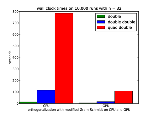
Figure 4: Plot corresponding to the data in Table 3. Observe that the rightmost bar representing times on a GPU with quad double arithmetic is shorter than the corresponding middle bar on a CPU with double double arithmetic. This plot illustrates the compensation of the overhead of quad double arithmetic (versus double double arithmetic) by a GPU.

The small speedup of 2.5 for complex double arithmetic in Table 3 shows that the fine granularity of the orthogonalization pays off only with multiprecision arithmetic. Comparing time on the GPU with quad double arithmetic to the time on the CPU with double double arithmetic we observe that the 115.6 seconds on one CPU core is of the same magnitude as the 108.0 seconds on the GPU. Obtaining more accurate orthogonalizations in about the same time is quality up.

We obtain double digit speedups with complex double arithmetic for $n\geq 96$, see Table 4 and Figure 5.

Table 4: Wall clock times for 10,000 runs of the modified Gram-Schmidt method (each followed by one backsubstitution) in complex double arithmetic for various dimensions n on CPU and GPU, with corresponding speedups.

complex double arithmetic
$n$	CPU	GPU	speedup
16	2.01	4.11	0.49
32	14.61	6.52	2.24
48	47.80	11.11	4.30
64	112.60	15.38	7.32
80	217.52	22.89	9.50
96	373.06	30.43	12.26
112	589.35	40.82	14.44
128	876.11	49.10	17.84
144	1243.26	67.41	18.44
160	1701.57	80.42	21.16
176	2260.07	99.94	22.61
192	2932.15	116.90	25.08
208	3722.77	149.45	24.91
224	4641.71	172.30	26.94
240	5703.77	211.30	26.99
256	6935.10	234.29	29.60

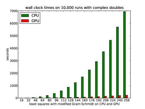
Figure 5: Plot corresponding to the data in Table 4, for dimensions ranging from $n=16$ to 256, with increments of 16.

Double digits speedups with complex double double arithmetic are obtained for $n\geq 48$. For complex quad double arithmetic we obtain a speedup of almost 10 for $n=48$. See Table 5 and Figure 6.

Comparing the first and the last execution time on the last line of Table 5 we observe the quality up. For $n=80$, the GPU computes the least squares solution that is twice as accurate in complex quad doubles as the solution in complex double doubles on the CPU, computed three times faster than the CPU, as $1841.07/597.47=3.08$.

Table 5: Wall clock times for 10,000 runs of the modified Gram-Schmidt method (each followed by one backsubstitution) in complex double double and complex quad double arithmetic, for various dimensions n on CPU and GPU, with corresponding speedups.

	complex double double			complex quad double
$n$	CPU	GPU	speedup	CPU	GPU	speedup
16	17.17	11.85	1.45	113.51	143.07	0.79
32	125.06	22.44	5.57	813.65	155.32	5.24
48	408.20	35.88	11.38	2556.36	266.55	9.59
64	952.35	55.18	17.26	6216.06	409.57	15.18
80	1841.07	79.11	23.27	12000.15	597.47	20.08

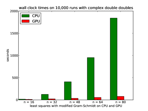
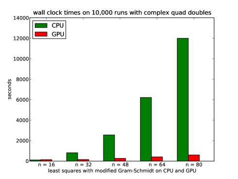
Figure 6: Plots corresponding to the data in Table 5, for dimensions $n=16,32,48,64,80$.

We end this paper with one sample of timings to illustrate the relationship with polynomial evaluation and differentiation (applying our parallel algorithms of [26]), see Figure 7. The total speedup is still sufficient to compensate for one level of extra precision.

Table 6: Wall clock times and overall speedups for 10,000 orthogonalizations on 32 random complex vectors of dimension 32 and for 10,000 polynomial evaluations and differentiations of polynomial system of 32 equations with 32 variables, with 32 monomials per polynomial, with 5 variables in each monomial, with variable degrees uniformly taken from $\{1,2,3,4,5\}$.

precision	CPU PE	GPU PE	speedup
complex double	11.0 sec	1.3 sec	8.5
complex double double	66.0 sec	2.1 sec	31.4
complex quad double	396.0 sec	14.2 sec	27.9
precision	CPU MGS	GPU MGS	speedup
complex double	13.4 sec	5.3 sec	2.5
complex double double	115.6 sec	16.5 sec	7.0
complex quad double	785.0 sec	108.0 sec	7.0
precision	CPU PE+MGS	GPU PE+MGS	speedup
complex double	24.4 sec	6.6 sec	3.7
complex double double	181.6 sec	18.6 sec	9.8
complex quad double	1181.0 sec	122.2 sec	9.7

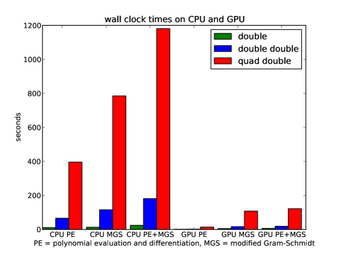
Figure 7: Plot corresponding to the data in Table 6. Observe that the rightmost bars representing times on a GPU with quad double arithmetic are shorter than the corresponding middle bars on a CPU with double double arithmetic. This plot illustrates the compensation of the overhead of quad double arithmetic (versus double double arithmetic) by a massively parallel algorithm on a GPU.

9 Conclusions

Using a massively parallel algorithm for the modified Gram-Schmidt orthogonalization on a NVIDIA Tesla C2050 Computing Processor we can compensate for the cost of one extra level of precision, even for modest dimensions, using a fine granularity. For larger dimensions we obtain double digit speedups and the GPU computes solutions, twice as accurate faster than the CPU.

References

- [1] S.G. Akl. Superlinear performance in real-time parallel computation. J. Supercomput., 29(1):89–111, 2004.
- [2] M. Anderson, G. Ballard, J. Demmel, and K. Keutzer. Communication-avoiding QR decomposition for GPUs. In Proceedings of the 2011 IEEE International Parallel Distributed Processing Symposium (IPDPS 2011), pages 48–58. IEEE Computer Society, 2011.
- [3] M.J Anderson, D. Sheffield, and K. Keutzer. A predictive model for solving small linear algebra problems in GPU registers. In Proceedings of the 2012 IEEE International Parallel Distributed Processing Symposium (IPDPS 2012), pages 2–13. IEEE Computer Society, 2012.
- [4] T.J. Dekker. A floating-point technique for extending the available precision. Numer. Math., 18(3):224–242, 1971.
- [5] G.H. Golub and C.F. Van Loan. Matrix Computations. The Johns Hopkins University Press, third edition, 1996.
- [6] Y. Hida, X.S. Li, and D.H. Bailey. Algorithms for quad-double precision floating point arithmetic. In 15th IEEE Symposium on Computer Arithmetic (Arith-15 2001), pages 155–162. IEEE Computer Society, 2001.
- [7] N.J. Higham. Accuracy and Stability of Numerical Algorithms. SIAM, 1996.
- [8] A. Kerr, D. Campbell, and M. Richards. QR decomposition on GPUs. In Proceedings of 2nd Workshop on General Purpose Processing on Graphics Processing Units (GPGPU’09), pages 71–78. ACM, 2009.
- [9] D.B. Kirk and W.W. Hwu. Programming Massively Parallel Processors. A Hands-on Approach. Morgan Kaufmann, 2010.
- [10] R.A. Klopotek and J. Porter-Sobieraj. Solving systems of polynomial equations on a GPU. In Preprints of the Federated Conference on Computer Science and Information Systems, pages 567–572, 2012.
- [11] T.Y. Li. Numerical solution of polynomial systems by homotopy continuation methods. In Handbook of Numerical Analysis. Volume XI. Special Volume: Foundations of Computational Mathematics, pages 209–304. North-Holland, 2003.
- [12] F.J. Linger. Efficient Gram-Schmidt orthonormalisation on parallel computers. Communications in Numerical Methods in Engineering, 16(1):57–66, 2000.
- [13] M. Lu, B. He, and Q. Luo. Supporting extended precision on graphics processors. In Proceedings of the Sixth International Workshop on Data Management on New Hardware (DaMoN 2010), pages 19–26, 2010.
- [14] M.M. Maza and W. Pan. Solving bivariate polynomial systems on a GPU. Journal of Physics: Conference Series, 341, 2011. Proceedings of High Performance Computing Symposium 2011, Montreal, 15-17 June 2011.
- [15] B. Milde and M. Schneider. Parallel implementation of classical Gram-Schmidt orthogonalization on CUDA graphics cards. Available via https://www.cdc.informatik.tu-darmstadt.de /de/cdc/personen/michael-schneider.
- [16] D. Mukunoki and D. Takashashi. Implementation and evaluation of triple precision BLAS subroutines on GPUs. In Proceedings of the 2012 IEEE 26th International Parallel and Distributed Processing Symposium Workshops, pages 1372–1380. IEEE Computer Society, 2012.
- [17] D.P. O’Leary and P. Whitman. Parallel QR factorization by Householder and modified Gram-Schmidt algorithms. Parallel Computing, 16(1):99–112, 1990.
- [18] D.N. Priest. On Properties of Floating Point Arithmetics: Numerical Stability and the Cost of Accurate Computations. PhD thesis, University of California at Berkeley, 1992.
- [19] G. Rünger and M. Schwind. Comparison of different parallel modified Gram-Schmidt algorithms. In Proceedings of the 11th international Euro-Par conference on Parallel Processing (Euro-Par’05), pages 826–836. Springer-Verlag, 2005.
- [20] H.-J. Su, J.M. McCarthy, M. Sosonkina, and L.T. Watson. Algorithm 857: POLSYS_GLP: A parallel general linear product homotopy code for solving polynomial systems of equations. ACM Trans. Math. Softw., 32(4):561–579, 2006.
- [21] S. Tomov, R. Nath, H. Ltaief, and J. Dongarra. Dense linear algebra solvers for multicore with GPU accelerators. In Proceedings of the IEEE International Symposium on Parallel and Distributed Processing Workshops (IPDSW 2010), pages 1–8. IEEE Computer Society, 2010.
- [22] L.N. Trefethen and R.S. Schreiber. Average-case stability of Gaussian elimination. SIAM J. Matrix Anal. Appl., 11(3):335–360, 1990.
- [23] J. Verschelde. Algorithm 795: PHCpack: A general-purpose solver for polynomial systems by homotopy continuation. ACM Trans. Math. Softw., 25(2):251–276, 1999.
- [24] J. Verschelde and G. Yoffe. Quality up in polynomial homotopy continuation by multithreaded path tracking. Preprint arXiv:1109.0545v1 [cs.DC] 2 Sep 2011.
- [25] J. Verschelde and G. Yoffe. Polynomial homotopies on multicore workstations. In Proceedings of the 4th International Workshop on Parallel Symbolic Computation (PASCO 2010), pages 131–140. ACM, 2010.
- [26] J. Verschelde and G. Yoffe. Evaluating polynomials in several variables and their derivatives on a GPU computing processor. In Proceedings of the 2012 IEEE 26th International Parallel and Distributed Processing Symposium Workshops, pages 1391–1399. IEEE Computer Society, 2012.
- [27] T. Yokozawa, D. Takahashi, T. Boku, and M. Sato. Efficient parallel implementation of classical Gram-Schmidt orthogonalization using matrix multiplication. In Parallel Matrix Algorithms and Applications (PMAA 2006), pages 37–38, 2006.