Abstract

A recent work on the resummation of fermionic in-medium ladder diagrams to all orders is extended by considering the effective range correction in the s-wave interaction and a (spin-independent) p-wave contact-interaction. A two-component recursion generates the in-medium T-matrix at any order when off-shell terms spoil the factorization of multi-loop diagrams. The resummation to all orders is achieved in the form of a geometrical series for the particle-particle ladders, and through an arctangent-function for the combined particle-particle and hole-hole ladders. One finds that the effective range correction changes the results in the limit of large scattering length considerably, with the effect that the Bertsch parameter $\xi_{n}$ nearly doubles. Applications to the equation of state of neutron matter at low density are also discussed. For the p-wave contact-interaction the resummation to all orders is facilitated by decomposing tensorial loop-integrals with a transversal and a longitudinal projector. The enhanced attraction provided by the p-wave ladder series has its origin mainly in the coherent sum of Hartree and Fock contributions.

PACS: 05.30.Fk, 12.20.Ds, 21.65+f, 25.10.Cn

1 Introduction and summary

Dilute degenerate many-fermion systems with large scattering lengths are of interest, e.g. for modeling the low-density behavior of nuclear and neutron star matter. Because of the possibility to tune magnetically atomic interactions, ultracold fermionic gases provide an exceptionally valuable tool to explore the non-perturbative many-body dynamics involved in the crossover from the superconducting to the Bose-Einstein condensed state (for a recent comprehensive review of this fascinating field, see ref.[1]). Of particular interest in this context is the so-called unitary limit in which the two-body interaction has the critical strength to support a bound-state at zero energy. As a consequence of the diverging scattering length, $a\to\infty$, the strongly interacting many-fermion system becomes scale-invariant. Its ground-state energy is then determined by a single universal number, the so-called Bertsch parameter $\xi$, which measures the ratio of the energy per particle $\bar{E}(k_{f})^{(\infty)}$ to that of a free Fermi gas $\bar{E}(k_{f})^{(0)}=3k_{f}^{2}/10M$. Here, $k_{f}$ denotes the Fermi momentum and $M$ the fermion mass.

The calculation of $\xi$ is an intrinsically non-perturbative problem which has been approached by numerical quantum Monte Carlo simulations. As the state of the art, a value of $\xi\simeq 0.38$ emerges at present [2, 3]. It is consistent with a recent precision measurement of the equation of state by the MIT group, which gives $\xi=0.37\pm 0.01$ [4] (extrapolating to zero temperature). Among the analytical approaches let us mention the $\epsilon$-expansion by Nishida and Son [5], where $\epsilon=4-d$ with $d$ the number of space dimensions. A naive extrapolation to $d=3$ gives $\xi=0.475$, but with inclusion of higher order corrections and Pade interpolations between the (otherwise diverging) expansions around $d=2$ and $d=4$, a good value of $\xi=0.38\pm 0.01$ could be obtained (see chapter 7 in ref.[1]). Because of the very large neutron-neutron scattering length $a_{nn}\simeq 19\,$fm, neutron matter at low densities is supposed to be a Fermi gas close to the unitary limit. Quantum Monte Carlo simulation [6, 7] and other sophisticated many-body calculations of neutron matter give indications for a value of $\xi_{n}\simeq 0.5$.

In a recent work [8] the complete resummation of the (combined) particle-particle and hole-hole ladder diagrams generated by a contact-interaction proportional to the scattering length $a$ has been achieved. A key to the solution of this (restricted) problem has been a different organization of the many-body calculation from the start. Instead of treating (propagating) particles and holes separately, these are kept together and the difference to the propagation in vacuum is measured by a “medium-insertion”. The following identical rewriting of the (non-relativistic) particle-hole propagator:

$$G(p_{0},\vec{p}\,) = {i\,\theta(|\vec{p}\,|-k_{f})\over p_{0}-\vec{p}^{\,2}/2M+i\epsilon}+{i\,\theta(k_{f}-|\vec{p}\,|)\over p_{0}-\vec{p}^{\,2}/2M-i\epsilon}$$ (1)

$$= {i\over p_{0}-\vec{p}^{\,2}/2M+i\epsilon}-2\pi\,\delta(p_{0}-\vec{p}^{\,2}/2M)\,\theta(k_{f}-|\vec{p}\,|)\,,$$

explains the basic principle of the approach. In that organizational scheme the pertinent in-medium loop is complex-valued, and therefore the contribution to the energy per particle $\bar{E}(k_{f})$ at order $a^{n}$ is not directly obtained from the $(n-1)$-th power of the in-medium loop (see Fig. 1). However, after reinstalling the symmetry factors $1/(j+1)$ which belong to diagrams with $j+1$ double medium-insertions, a real-valued expression is obtained for all orders $a^{n}$. Known results about the low-density expansion [9, 10] up to and including order $a^{4}$ could be reproduced with improved numerical accuracy. The emerging series in $ak_{f}$ could even be summed to all orders in the form of a double-integral over an arctangent-function. In that explicit representation the unitary limit, $a\to\infty$, could be taken straightforwardly and the value $\xi=0.507$ has been found for the Bertsch parameter [8]. This number is to be compared with the value $\xi^{(pp)}\simeq 0.237$ resulting from a resummation of particle-particle ladder diagrams only [11]. Clearly, since only the (infinite) subset of particle-hole ladder diagrams [8] is computed in the normal phase one cannot expect accurate results for the unitary Fermi gas, whose true ground state is a superfluid. But interestingly, extrapolations of the equation of state of the unitary Fermi gas from finite to zero temperature, which smoothly pass over the pairing transition at $T_{c}$ give indications for a Bertsch parameter $\xi_{n}\simeq 0.5$ in the normal phase [1, 4, 12]. In comparison to this synthetic result, the value $\xi_{n}=0.507$ of ref.[8] appears to be a rather good finding.

The purpose of the present paper is to extend the resummation method of ref.[8] by including the effective range correction in the s-wave interaction and by considering also a spin-independent p-wave contact interaction to all orders. The effective range correction to a contact-interaction (proportional to the scattering length $a$) has been studied first by Schäfer et al. in ref.[11] for the resummed particle-particle ladder series. The implications of this correction on the equation of state have, however, not been explored in much detail and only rough perturbative estimates have been given. In a related work by Schwenk and Pethick [13] it has been argued that the inclusion of the effective range $r_{s}=2.75\,$fm leads to an improved description of neutron matter at low densities. Their implementation of the effective range $r_{s}$ into the particle-particle ladder series assumes a form similar to the effective range expansion for neutron-neutron scattering in free space. However, a proper diagrammatic calculation [11] shows that in the medium the combination of scattering length $a$ and effective range $r_{s}$ produces additional (density-dependent) off-shell terms which spoil the factorization of multi-loop diagrams. A resummation of the particle-particle ladder diagrams to all orders in the form of a geometrical series is still possible, but it differs from the expression suggested by the effective range expansion in vacuum.

The present paper is organized as follows: In section 2 we perform the resummation of fermionic in-medium ladder diagrams for a contact-interaction that includes the effective range $r_{s}$. It is demonstrated that a two-component recursion generates the in-medium T-matrix at any order when off-shell terms spoils the direct factorization of multi-loop diagrams. The resummation to all orders is still achieved in the form of a geometrical series for the particle-particle ladders, and through an arctangent-function for the combined particle-particle and hole-hole ladders. The second more complicated case involves yet a (combinatorial) conjecture because the arctangent-series could be verified so far with diagrammatic methods only to some finite order. One finds that the effective range correction changes the results in the limit of large scattering length $a\to\infty$ considerably, with the effect that the Bertsch parameter $\xi_{n}$ (for the normal phase) increases. For the combined particle-hole ladder series one gets $\xi_{n}(r_{s}\neq 0)=0.876$, and for the resummed particle-particle ladder series alone the value is $\xi_{n}^{(pp)}(r_{s}\neq 0)\simeq 0.43$. Applications of these resummation results to the equation of state of neutron matter at low density are presented and discussed in comparison. Section 3 deals with the analogous resummation to all orders for a (spin-independent) p-wave contact-interaction. In this case the factorization of multi-loop diagrams is achieved more directly by decomposing tensorial loop-integrals into a transversal and a longitudinal part. These two parts decouple and can therefore be resummed separately through an arctangent-function or a geometrical series. The enhanced attraction provided by the p-wave ladder series (in the limit of large scattering volume $a_{1}^{3}\to\infty$) has its origin mainly in the coherent sum of Hartree and Fock contributions. In the appendix analytical results for the resummation of particle-hole diagrams to all orders are presented for a two-component fermionic system (such as nuclear matter) with two different scattering lengths, $a_{s}$ and $a_{t}$, in the presence of an isospin-asymmetry, $k_{n}>k_{p}$. A special case of such an asymmetric system is the (unitary) Fermi gas in the spin-unbalanced configuration.

Presumably the results of the present paper are contained (to a certain extent) as special cases in the work of Lacour et al. [14]. In that paper non-perturbative methods for chiral effective field theory of finite density nuclear systems have been developed. The approach is based on a partial wave representation of leading order nucleon-nucleon interactions which are summed to all orders in the medium. A detailed comparison of the present results (obtained from simple contact-interactions) with those of ref.[14] is certainly interesting, but this requires an extensive communication between both groups in order to translate the different formalisms correctly into each other and to establish the common range of applicability.

The study of strongly-coupled fermionic many-body systems (such as neutron matter) at low density with quantum Monte Carlo simulations [15, 16, 17] is presently an active research area. The analytical results of the present work, which of course cover only a restricted part of the many-body dynamics, could be potentially useful for interpreting these numerical simulations.

2 Resummation with inclusion of the effective range

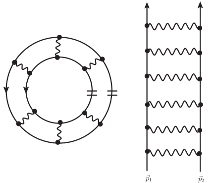
Figure 1: Left: Closed multi-loop diagram representing a contribution to the energy density. Right: Planar ladder diagram obtained by opening at a minimal pair of adjacent medium-insertions. Wiggly lines symbolize contact-interactions.

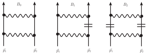
Figure 2: In-medium loop organized in the number of medium-insertions (=). The central diagram has a reflected partner. The external momenta $|\vec{p}_{1,2}|<k_{f}$ are inside the Fermi sphere.

In this section we develop methods which allow for a complete resummation of fermionic in-medium ladder diagrams for an s-wave contact-interaction that includes the effective range correction. We recall from ref.[8] that after opening a closed multi-loop diagram (representing the energy density) at adjacent medium-insertions a planar ladder diagrams results (see Fig. 1). If the contact-interaction is momentum-independent all these (open) multi-loop diagrams factorize into powers of the in-medium loop. In the ordering scheme implied by eq.(1) the in-medium loop is composed of contributions with zero, one, and two medium-insertions (see Fig. 2). The first part represents the rescattering in the vacuum and the other two parts incorporate systematically the (Pauli-blocking) effects due to the fermionic medium. The resulting in-medium loop is complex-valued, but after a careful combinatoric analysis of the closed multi-loop diagrams a real-valued expression for the energy density is obtained at each order. In the next step the complete resummation to all orders can be performed through an arctangent-function that depends on both the real and imaginary part of the in-medium loop.

The aim is to generalize this novel approach to an s-wave contact-vertex:

$$C_{0}+C_{2}(\vec{q}_{\rm in}^{\,2}+\vec{q}_{\rm out}^{\,2})\,,$$ (2)

which includes the effective range correction. Here, $\vec{q}_{\rm in}$ and $\vec{q}_{\rm out}$ denote half of the momentum difference in the initial and the final state, respectively. Such a form of the contact-vertex is actually dictated by Galilei invariance. The relations of the coupling constants $C_{0}$ and $C_{2}$ to the scattering length $a$ and the effective range parameter $r_{s}$ are:

$$C_{0}={4\pi a\over M}\,,\qquad C_{2}=-{\pi a^{2}r_{s}\over M}\,.$$ (3)

Note that we are choosing the sign-convention such that a positive scattering length $a>0$ corresponds to attraction. The repeated rescatterings via the contact-vertex eq.(2) in vacuum (i.e. the left diagram in Fig. 2 iterated to all orders) leads to an s-wave phase shift $\delta_{0}(q)$ of the form:

$$\tan\delta_{0}(q)=a\,q-{a^{2}r_{s}\over 2}q^{3}\,,$$ (4)

with $q$ the center-of-mass momentum. We are using dimensional regularization, where all (scale-free) power divergences are set to zero: $\int_{0}^{\infty}dl\,l^{n}=0$. The real part of the in-medium loop is generated by the central diagram in Fig. 2. The pertinent integration formula for the real part reads:

$$-\!\!\!\!\!\!\int\!{d^{3}l\over(2\pi)^{3}}\,{-M\over\vec{l}^{\,2}-\vec{q}^{\,2}}\Big{\{}\theta(k_{f}-|\vec{P}-\vec{l}\,|)+\theta(k_{f}-|\vec{P}+\vec{l}\,|)\Big{\}}\dots\,,$$ (5)

with the factors from the lower and upper interaction-vertex to be inserted at the place of the dots. Here, we have introduced the half sum $\vec{P}=(\vec{p}_{1}+\vec{p}_{2})/2$ and half difference $\vec{q}=(\vec{p}_{1}-\vec{p}_{2})/2$ of the external momenta $|\vec{p}_{1,2}|<k_{f}$ inside the Fermi sphere. All three diagrams in Fig. 2 contribute to imaginary part of the in-medium loop and the pertinent integration formula reads:

$$\int\!\!{d^{3}l\over(2\pi)^{3}}\,M\pi\,\delta(\vec{l}^{\,2}-\vec{q}^{\,2})\,\theta(k_{f}-|\vec{P}-\vec{l}\,|)\,\theta(k_{f}-|\vec{P}+\vec{l}\,|)\dots\,.$$ (6)

Note that we have left out a term $[1-\theta(\dots)][1-\theta(\dots)]$ which vanishes on-shell $(\vec{l}^{\,2}=\vec{q}^{\,2})$ due to energy conservation and Pauli-blocking (see eq.(8) in ref.[8]). Let us now analyze more closely the one-loop diagrams in Fig. 2 with two momentum-dependent $C_{0,2}$ vertices. For the lower vertex the assignment $\vec{q}_{\rm in}=\vec{q}$, $\vec{q}_{\rm out}=\vec{l}$ with $\vec{l}$ the loop-momentum holds, while for the upper vertex it is $\vec{q}_{\rm in}=\vec{l}$, $\vec{q}_{\rm out}=\vec{q}$. Actually, if a further loop is considered the second $\vec{q}_{\rm out}$ is set to the new loop momentum $\vec{l}\,^{\prime}$ and therefore this second $\vec{q}_{\rm out}$ should not be fixed immediately. One recognizes that the product of interaction vertices contains terms proportional to $\vec{l}^{\,2}$ and $\vec{l}^{\,4}$. With inclusion of the energy denominator in eq.(5) these can be decomposed into on-shell vertices ($\vec{l}^{\,2}\to\vec{q}^{\,2}$) and polynomial off-shell pieces:

$${\vec{l}^{\,2}\over\vec{l}^{\,2}-\vec{q}^{\,2}}={\vec{q}^{\,2}\over\vec{l}^{\,2}-\vec{q}^{\,2}}+1\,,\qquad{\vec{l}^{\,4}\over\vec{l}^{\,2}-\vec{q}^{\,2}}={\vec{q}^{\,4}\over\vec{l}^{\,2}-\vec{q}^{\,2}}+\vec{l}^{\,2}+\vec{q}^{\,2}\,.$$ (7)

These off-shell terms produce additional real-valued contributions which enter into the next loop, where by the same mechanism new off-shell terms are generated, and so on. The factorization of multi-loop diagrams into powers of the in-medium loop gets thus spoiled by the presence of the $C_{2}$ coupling proportional to the effective range $r_{s}$. Although it looks complicated at first sight, one can recursively follow the continuous proliferation of off-shell terms by simultaneously keeping track of two quantities: the (on-shell) in-medium T-matrix $T_{n}$ and the coefficient $\beta_{n}$ of $\vec{q}_{\rm out}^{\,2}$. Injecting the expression $T_{n}+\beta_{n}(\vec{q}_{\rm out}^{\,2}-\vec{q}^{\,2})$ at order $n$ with $\vec{q}_{\rm out}\to\vec{l}$ and concatenating it through the in-medium loop with one additional $C_{0,2}$ vertex produces as an output the same expression at order $n+1$. As a transparent result one deduces a linear two-component recursion of the form:

$$\left(\!\!\begin{array}[]{c}T_{n+1}\\ \beta_{n+1}\\ \end{array}\!\!\right)={\cal M}\left(\!\!\begin{array}[]{c}T_{n}\\ \beta_{n}\\ \end{array}\!\!\right)\,,$$ (8)

with the starting values $T_{1}=C_{0}+2C_{2}\vec{q}^{\,2}$ and $\beta_{1}=C_{2}$. The pertinent $2\times 2$ matrix ${\cal M}$ reads:

$${\cal M}=\left(\!\!\begin{array}[]{cc}(C_{0}+2C_{2}\vec{q}^{\,2}){\cal L}+C_{2}X&(C_{0}+C_{2}\vec{q}^{\,2})X+C_{2}Y\\ C_{2}{\cal L}&C_{2}X\\ \end{array}\!\!\right)\,,$$ (9)

with $X,\,Y$ the off-shell terms originating from Fermi sphere integrals over the terms $1,\,\vec{l}^{\,2}$ in eq.(7) and ${\cal L}$ the complex-valued in-medium loop (see eqs.(14-17)). Although the polynomial expressions for the in-medium T-matrices $T_{n}$ get increasingly more complicated with increasing $n$, their total sum can be easily calculated with the help of matrix-inversion:

$$\sum\limits_{n=1}^{\infty}T_{n}=(1,0)\,\Big{[}{\bf 1}-{\cal M}\Big{]}^{-1}\!\left(\!\!\begin{array}[]{c}C_{0}+2C_{2}\vec{q}^{\,2}\\ C_{2}\\ \end{array}\!\!\right)=\Big{[}V_{\rm eff}^{-1}-{\cal L}\Big{]}^{-1}=\sum\limits_{n=1}^{\infty}V_{\rm eff}^{n}\,{\cal L}^{n-1}\,.$$ (10)

The second equality reveals that the reciprocal of this infinite series splits off instantaneously the complex-valued in-medium loop ${\cal L}$ and the third equality shows that the result is identical to a geometrical series with an effective density and momentum dependent potential:

$$V_{\rm eff}={C_{0}+2C_{2}\vec{q}^{\,2}+C_{2}^{2}(Y-X\vec{q}^{\,2})\over(1-C_{2}X)^{2}}\,.$$ (11)

The beginning and the end of eq.(10) represent a remarkable identity. It means that although the individual multi-loop diagrams did not factorize, their total sum agrees exactly with a geometrical series one would have obtained by using the effective potential $V_{\rm eff}$ and assuming factorization. Note that $V_{\rm eff}$ depends in a non-linear way on the off-shell term $X$ and when dropping the effective range $C_{2}=0$ one recovers $V_{\rm eff}=C_{0}=4\pi a/M$. A resummation of the in-medium T-matrix with inclusion of all partial waves has been proposed in section 4.2 of ref.[14] (assuming on-shell factorization).

The intermediate resummation result in eq.(10) does not yet provide the correct integrand for computing the energy per particle $\bar{E}(k_{f})$ because it is complex-valued. Following the instructive diagrammatic analysis in section 4 of ref.[8] we make the conjecture that the proper resummation of in-medium ladder diagrams to all orders is achieved by the substitution:

$${1\over V_{\rm eff}^{-1}-{\cal L}}\rightarrow{1\over{\rm Im}{\cal L}}\,\arctan{{\rm Im}{\cal L}\over V_{\rm eff}^{-1}-{\rm Re}{\cal L}}\,.$$ (12)

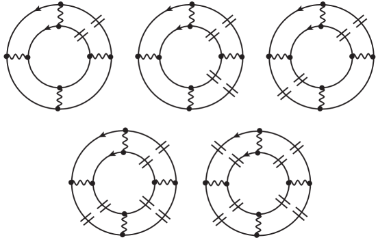
Figure 3: In-medium ladder diagrams contributing to the energy density at fourth order. The third and fifth diagram have symmetry factors $1/2$ and $1/4$, respectively.

We have verified by a detailed diagrammatic analysis that the arctangent-prescription in eq.(12) leads to the correct result in a perturbative expansion in the coupling constants $C_{0,2}$ (at least) up to sixth order. In order to present an example, the corresponding set of diagrams at fourth order is shown in Fig. 3. These decorated diagrams have symmetry factors $1,1,1/2,1$ and $1/4$, in the order shown. Taking these symmetry factors into account the integrand for computing the energy density at fourth order has the form:

$$T_{4}^{*}+T_{3}^{*}T_{1}(2i\,{\rm Im}{\cal L})+{1\over 2}(T_{2}^{*})^{2}(2i\,{\rm Im}{\cal L})+T_{2}^{*}(T_{1})^{2}(2i\,{\rm Im}{\cal L})^{2}+{1\over 4}(T_{1})^{4}(2i\,{\rm Im}{\cal L})^{3}\,,$$ (13)

where $T_{n}^{*}$ denotes the complex-conjugate  of the $n$-th order T-matrix $T_{n}$ to be calculated recursively via eq.(8). This sum of five complex terms is indeed real-valued and it agrees exactly with the expression one obtains by expanding the arctangent-function in eq.(12) to fourth power in the couplings $C_{0,2}$. The relevant real-valued integrands at second and third order are: $T_{2}^{*}+{1\over 2}(T_{1})^{2}(2i\,{\rm Im}{\cal L})$ and $T_{3}^{*}+T_{2}^{*}T_{1}(2i\,{\rm Im}{\cal L})+{1\over 3}(T_{1})^{3}(2i\,{\rm Im}{\cal L})^{2}$. Going step by step perturbatively to higher $n$ is in principle straightforward, it requires to check in each case the equality of two very long polynomial expressions. A complete verification of eq.(12) to all orders $n$ requires the consideration of all possible partitions $(n_{1},n_{2},\dots,n_{j})$ of $n=n_{1}+n_{2}+\dots+n_{j}$ together with their symmetry factors. The sequence $(n_{1},n_{2},\dots,n_{j})$ counts here the numbers of contact-interactions between consecutive double medium-insertions (see Fig. 3). Since the partitions of $n$ are in one-to-one correspondence to the inequivalent irreducible representations of the permutation group $S_{n}$ there might exist some sophisticated combinatorial identities, which could help to solve this problem completely.

Before turning to the final result for the resummed energy per particle we give the explicit analytical expressions for the off-shell terms:

$$X=-{Mk_{f}^{3}\over 3\pi^{2}}\,,\qquad Y=-{Mk_{f}^{5}\over 15\pi^{2}}(5s^{2}+3)\,,$$ (14)

and for the complex-valued in-medium loop:

$${\cal L}={Mk_{f}\over 4\pi^{2}}\Big{\{}-R(s,\kappa)+i\pi\,I(s,\kappa)\Big{\}}\,.$$ (15)

The dimensionless variables $s=|\vec{p}_{1}+\vec{p}_{2}|/2k_{f}$ and $\kappa=|\vec{p}_{1}-\vec{p}_{2}|/2k_{f}$ fulfil the constraint $s^{2}+\kappa^{2}<1$, since $|\vec{p}_{1,2}|<k_{f}$. The dimensionless real part $R(s,\kappa)$ and imaginary part $I(s,\kappa)$ introduced in eq.(15) have the form [8]:

$$R(s,\kappa)=2+{1\over 2s}[1-(s+\kappa)^{2}]\ln{1+s+\kappa\over|1-s-\kappa|}+{1\over 2s}[1-(s-\kappa)^{2}]\ln{1+s-\kappa\over 1-s+\kappa}\,,$$ (16)

$$I(s,\kappa)=\kappa\,\theta(1-s-\kappa)+{1\over 2s}(1-s^{2}-\kappa^{2})\,\theta(s+\kappa-1)\,.$$ (17)

The same expression for the in-medium loop has been derived in appendix C of ref.[14]. With these ingredients the resummed energy per particle is readily calculated. The 2-ring Hartree and 1-ring Fock diagram add up with their spin-factors as $4-2=2$. One uses the reduction formula eq.(15) in ref.[8] for the integral over two Fermi spheres $|\vec{p}_{1,2}|<k_{f}$ to cancel yet the factor $1/{\rm Im}{\cal L}$ in eq.(12), and obtains the following expression for the interaction energy per particle:

$$\bar{E}(k_{f})=-{24k_{f}^{2}\over\pi M}\int\limits_{0}^{1}\!ds\,s^{2}\!\!\int\limits_{0}^{\sqrt{1-s^{2}}}\!\!d\kappa\,\kappa\,\arctan{\pi\,I(s,\kappa)\over\Omega(a,r_{s})^{-1}+R(s,\kappa)}\,,$$ (18)

with the auxiliary function:

$$\Omega(a,r_{s})={3ak_{f}\over(3\pi-a^{2}r_{s}k_{f}^{3})^{2}}\bigg{\{}{3\pi\over 2}(2-ar_{s}k_{f}^{2}\kappa^{2})+{a^{3}r_{s}^{2}k_{f}^{5}\over 20}(5\kappa^{2}-5s^{2}-3)\bigg{\}}\,,$$ (19)

depending on the physical parameters: scattering length $a$, effective range $r_{s}$ and Fermi momentum $k_{f}$. When dropping the effective range one recovers $\Omega(a,0)=ak_{f}/\pi$ and in the limit of large scattering length, $\lim\limits_{a\to\infty}\Omega(a,r_{s})=3(5\kappa^{2}-5s^{2}-3)/20$ becomes independent of $r_{s}k_{f}$. This comparison demonstrates that the limits $a\to\infty$ and $r_{s}\to 0$ do not commute. The arctangent-function occurring in eq.(18) refers to the usual branch with odd parity, $\arctan(-x)=-\arctan x$, and values in the interval $[-\pi/2,\pi/2]$. We note that the leading order correction involving the effective range, $\bar{E}(k_{f})^{(\rm lo)}=a^{2}r_{s}k_{f}^{5}/20\pi M$, agrees with the low-density expansion of ref.[9].

Since the unitary limit $a\to\infty$ can be performed straightforwardly for eq.(19) a first interest aims at the Bertsch parameter. A numerical evaluation of the double-integral in eq.(18) gives $\xi_{n}(r_{s}\neq 0)=0.876$, which is considerably larger than the value $\xi_{n}(r_{s}=0)=0.507$ for vanishing effective range. The reason for this feature are the off-shell terms $X,Y$ in eq.(11) which change the reciprocal effective interaction $V_{\rm eff}^{-1}$ drastically. Note that the ratio $C_{2}/C_{0}=-ar_{s}/4$ is large. The resummation formula given in eqs.(18,19) offers of course the possibility to study various other strong coupling limits $a\to\infty$, by imposing a certain relation between $a$ and $r_{s}$.

2.1 Particle-particle ladders only

In this subsection we adapt the previous methods to the particle-particle ladders series with inclusion of the effective range correction [11]. The particle-particle ladder diagrams are resummed via a geometrical series $(V_{\rm eff}^{-1}-{\cal L})^{-1}_{pp}$, in which the quantities $X,Y$ and ${\cal L}$ take on a different form. For particle-particle intermediate states only the integration region in eq.(5) changes effectively from the sum to the union of two partly overlapping Fermi spheres $|\vec{P}\pm\vec{l}\,|<k_{f}$. Performing these integrals, one finds for the $pp$ off-shell terms:

$$X_{pp}=-{Mk_{f}^{3}\over 12\pi^{2}}(1+s)^{2}(2-s)\,,\qquad Y_{pp}=-{Mk_{f}^{5}\over 60\pi^{2}}(1+s)^{3}(6-3s+s^{2})\,,$$ (20)

in the region $0<s<1$ of interest, and for the $pp$ in-medium loop:

$${\cal L}_{pp}=-{Mk_{f}\over 4\pi^{2}}F_{pp}(s,\kappa)\,,$$ (21)

with the familiar particle-particle bubble function ($s^{2}+\kappa^{2}<1)$:

$$F_{pp}(s,\kappa)=1+s-\kappa\ln{1+s+\kappa\over 1+s-\kappa}+{1\over 2s}(1-s^{2}-\kappa^{2})\ln{(1+s)^{2}-\kappa^{2}\over 1-s^{2}-\kappa^{2}}\,.$$ (22)

Putting these pieces together, one derives from the resummed particle-particle ladder diagrams the following expression for the energy per particle:

$$\bar{E}(k_{f})=-{24k_{f}^{2}\over M}\int\limits_{0}^{1}\!ds\,s^{2}\!\!\int\limits_{0}^{\sqrt{1-s^{2}}}\!\!d\kappa\,\kappa\,{I(s,\kappa)\over\Omega_{pp}(a,r_{s})^{-1}+F_{pp}(s,\kappa)}\Bigg{\}}\,,$$ (23)

with the auxiliary function:

$$\Omega_{pp}(a,r_{s}) = {3ak_{f}\over[12\pi-a^{2}r_{s}k_{f}^{3}(1+s)^{2}(2-s)]^{2}}\bigg{\{}24\pi(2-ar_{s}k_{f}^{2}\kappa^{2})$$ (24)

$$+a^{3}r_{s}^{2}k_{f}^{5}(1+s)^{2}\bigg{[}(2-s)\kappa^{2}+{1+s\over 5}(3s-6-s^{2})\bigg{]}\bigg{\}}\,,$$

depending on the physical parameters $a,r_{s}$ and $k_{f}$. Again, when dropping the effective range, $\Omega_{pp}(a,0)=ak_{f}/\pi$, and in the strong coupling limit $\Omega_{pp}(\infty,r_{s})=3[(1+s)(3s-6-s^{2})+5(2-s)\kappa^{2}]/[5(1+s)^{2}(2-s)^{2}]$ becomes independent of $r_{s}k_{f}$. Because of zeros in the denominator, the double-integral in eq.(23) is to be understood as a principal-value integral. In the actual numerical treatment we work with a cutting-function, ${\rm Cut}(x)=x$ for $|x|<N$, ${\rm Cut}(x)=0$ for $|x|>N$, in order to implement the symmetrical excision around the first-order poles and study the convergence behavior for large $N$. It is important to note that our result agrees exactly with eq.(13) in ref.[11] (after matching the conventions for the coupling constants $C_{0,2}$). The underlying structure of a geometrical series with an effective potential $V_{\rm eff}^{(pp)}$ and the reduction to an integral over the quarter unit-disc has seemingly not been recognized in that paper. Note that ref.[11] has investigated in addition the summable series of the particle-hole ring diagrams. For this subclass of diagrams (as well as for the isolated hole-hole ladder series) the energy per particle $\bar{E}(k_{f})$ diverges in the strong coupling limit $a\to\infty$ (see sections 3 and 4 in ref.[11]).

In the unitary limit $a\to\infty$, a numerical integration gives for the Bertsch parameter $\xi_{n}^{(pp)}(r_{s}\neq 0)\simeq 0.43$ which amounts to almost twice the value $\xi_{n}^{(pp)}(r_{s}=0)\simeq 0.237$ at vanishing effective range. The approach of Schwenk and Pethick [13] has employed the form $\Omega_{pp}(a,r_{s})^{-1}=\pi(1/ak_{f}+r_{s}k_{f}\kappa^{2}/2)$ as suggested by the effective range expansion in free space.

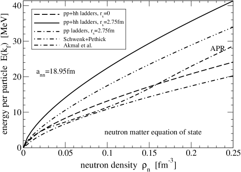
Figure 4: Energy per particle of neutron matter as a function of the neutron density $\rho_{n}=k_{f}^{3}/3\pi^{2}$. The line labelled APR stems from the sophisticated many-body calculation of ref.[18].

2.2 Application to low-density neutron matter

As an application we consider the equation of state of neutron matter. Due to the very large neutron-neutron scattering length $a_{nn}=(18.95\pm 0.40)\,$fm [19] neutron matter at low densities is supposed to be a Fermi gas close to the unitary limit. Fig. 4 shows the energy per particle of neutron matter as a function of the neutron density $\rho_{n}=k_{f}^{3}/3\pi^{2}$. The full and dashed line result from the resummation of (combined particle-hole) ladder diagrams eq.(18) with inclusion of the empirical effective range parameter $r_{s}=(2.75\pm 0.11)\,$fm and by dropping it, $r_{s}=0$. The resummation of the particle-particle ladders only leads to dashed-dotted line in Fig. 4 and the result of the approach by Schwenk and Pethick [13] is additionally included. In each case the sum of kinetic and interaction energy per particle $3k_{f}^{2}/10M+\bar{E}(k_{f})$ is plotted. The curve labeled APR stems from the sophisticated many-body calculation by the Urbana group [18], to be considered as a representative of realistic neutron matter calculations. In fact a recent calculation of neutron matter in chiral effective field theory with inclusion of subleading three-nucleon forces etc. leads to a very similar equation of state [20]. Only the lower two lines in Fig. 4 give a reasonable reproduction of the APR curve at low densities $\rho_{n}<0.2\,$fm^-3. Since the dimensionless variable $a_{nn}k_{f}$ reaches values up to $34.3$ in this density region the behavior of the total energy per particle $3k_{f}^{2}/10M+\bar{E}(k_{f})$ is almost entirely determined by the value of the Bertsch parameter $\xi_{n}$. Note that for a correct reproduction of the neutron matter equation of state at low densities it has to be close to $\xi_{n}\simeq 0.5$. The additional repulsive effects arising from hole-hole and mixed particle-hole ladders are recognizable as the difference between the full and dashed-dotted line in Fig. 4. Despite the deviations from the APR curve visible in Fig. 4, we reproduce the results of Schwenk and Pethick for densities $\rho_{n}<0.02\,$fm^-3 actually considered in ref.[13].

3 Resummation of p-wave contact interaction

In this section we extend the resummation method to a spin-independent p-wave contact-interaction. The pertinent contact-vertex obeying Galilei invariance reads:

$$C_{1}\,\vec{q}_{\rm in}\cdot\vec{q}_{\rm out}\,,$$ (25)

with the coupling constant $C_{1}$ related to the p-wave scattering volume $a_{1}^{3}$ by $C_{1}=12\pi a_{1}^{3}/M$. The repeated rescatterings via this contact-vertex in the vacuum (i.e. the left diagram in Fig. 2 iterated to all orders) leads to a p-wave phase shift of the form:

$$\tan\delta_{1}(q)=(a_{1}q)^{3}\,,$$ (26)

with $q$ the center-of-mass momentum and we have used the rule $\int_{0}^{\infty}dl\,l^{n}=0$ of dimensional regularization. In the in-medium loop two consecutive $C_{1}$ vertices introduce the factor $(\vec{q}_{\rm in}\cdot\vec{l}\,)(\vec{l}\cdot\vec{q}_{\rm out})$. We decompose the emerging tensorial integral over $l_{i}l_{j}$ into the transversal projector $\delta_{ij}-\hat{P}_{i}\hat{P}_{j}$ and the longitudinal projector $\hat{P}_{i}\hat{P}_{j}$, where $\vec{P}=(\vec{p}_{1}+\vec{p}_{2})/2$ (see Fig. 2). Since these are two orthogonal projectors the factorization of multi-loop diagrams holds separately for the transversal and longitudinal part of the tensor to be contracted with $q_{\rm in}^{i}q_{\rm out}^{j}$. In this decoupling procedure one encounters a transversal in-medium loop whose real and imaginary part read:

$$R_{\perp}(s,\kappa) = {2\over 3}-{s^{2}\over 4}+2\kappa^{2}+{(1-\kappa^{2})^{2}\over 4s^{2}}+{[(s+\kappa)^{2}-1]^{2}\over 16s^{3}}(s^{2}+\kappa^{2}-4s\kappa-1)$$ (27)

$$\times\ln{1+s+\kappa\over|1-s-\kappa|}+{[(s-\kappa)^{2}-1]^{2}\over 16s^{3}}(s^{2}+\kappa^{2}+4s\kappa-1)\ln{1+s-\kappa\over 1-s+\kappa}\,,$$

$$I_{\perp}(s,\kappa)=\kappa^{3}\,\theta(1-s-\kappa)+{1-s^{2}-\kappa^{2}\over 16s^{3}}\Big{[}12s^{2}\kappa^{2}-(1-s^{2}-\kappa^{2})^{2}\Big{]}\,\theta(s+\kappa-1)\,,$$ (28)

as well as a longitudinal in-medium loop whose real and imaginary part read:

$$R_{\parallel}(s,\kappa) = {8\over 3}+{s^{2}\over 2}+2\kappa^{2}-{(1-\kappa^{2})^{2}\over 2s^{2}}+\bigg{[}{(1-s^{2}-\kappa^{2})^{3}\over 8s^{3}}-\kappa^{3}\bigg{]}$$ (29)

$$\times\ln{1+s+\kappa\over|1-s-\kappa|}+\bigg{[}{(1-s^{2}-\kappa^{2})^{3}\over 8s^{3}}+\kappa^{3}\bigg{]}\ln{1+s-\kappa\over 1-s+\kappa}\,,$$

$$I_{\parallel}(s,\kappa)=\kappa^{3}\,\theta(1-s-\kappa)+{(1-s^{2}-\kappa^{2})^{3}\over 8s^{3}}\,\theta(s+\kappa-1)\,.$$ (30)

The diagrammatic analysis in section 4 of ref.[8] emphasizing the important role of symmetry factors instructs that for the energy density the proper resummation to all orders is achieved through an arctangent-function. By using the operator identity for projectors, $\arctan(\Pi_{\perp}x_{\perp}+\Pi_{\parallel}x_{\parallel})=\Pi_{\perp}\arctan x_{\perp}+\Pi_{\parallel}\arctan x_{\parallel}$, the transversal and longitudinal parts get separated completely. A special feature of the (resummed) p-wave contact-interaction is that the 2-ring Hartree and 1-ring Fock diagram add up with their spin-factors as $4+2=6$. While $\vec{q}_{\rm in}=(\vec{p}_{1}-\vec{p}_{2})/2=\vec{q}$ for both, there is a sign difference in $\vec{q}_{\rm out}=\pm\,\vec{q}$ for the Hartree and Fock contributions. Putting all pieces together one finds from the resummed ladder diagrams with a (spin-independent) p-wave contact-interaction the following expression for the energy per particle:

$$\bar{E}(k_{f}) = -{72k_{f}^{2}\over\pi M}\int\limits_{0}^{1}\!ds\,s^{2}\!\!\int\limits_{0}^{\sqrt{1-s^{2}}}\!\!d\kappa\,\kappa\,\Bigg{\{}2\arctan{I_{\perp}(s,\kappa)\over(a_{1}k_{f})^{-3}+\pi^{-1}R_{\perp}(s,\kappa)}$$ (31)

$$\qquad\qquad\qquad\qquad\qquad\,\,+\arctan{I_{\parallel}(s,\kappa)\over(a_{1}k_{f})^{-3}+\pi^{-1}R_{\parallel}(s,\kappa)}\Bigg{\}}\,.$$

The factor $2$ is reminiscent of two transversal versus one longitudinal degree of freedom. Another interesting feature is that the imaginary parts of the transversal and longitudinal loop functions, $I_{\perp}(s,\kappa)$ and $I_{\parallel}(s,\kappa)$ in eqs.(28,30), appear (with a prefactor $s^{2}\kappa$) as weighting functions in the reduction of integrals over two Fermi spheres $|\vec{p}_{1,2}|<k_{f}$.

As a first application let us consider the low-density expansion of $\bar{E}(k_{f})$ in eq.(31), which reads:

$$\bar{E}(k_{f})={k_{f}^{2}\over 2M}\bigg{\{}-{9\over 5\pi}(a_{1}k_{f})^{3}+{1033-156\ln 2\over 385\pi^{2}}(a_{1}k_{f})^{6}+\dots\bigg{\}}\,\,.$$ (32)

The linear term in the scattering volume $a_{1}^{3}$ agrees with ref.[9] (after matching conventions $a_{p}=-3^{1/3}a_{1}$) while the second order term with its peculiar numerical coefficient is new. It is also straightforward to perform the strong coupling limit $a_{1}\to\infty$ for $\bar{E}(k_{f})$ in eq.(31). One finds $\bar{E}(k_{f})^{(\infty)}=(3k_{f}^{2}/10M)(-1.948)$, corresponding to almost minus twice the free Fermi gas energy and therefore an instability of the system. The basic reason for this overly strong p-wave attraction is the enhancement factor $3$ from the coherent sum of Hartree and Fock terms. In the case of a strong s-wave interaction the number multiplying the free Fermi gas energy $3k_{f}^{2}/10M$ is $\xi_{n}-1=-0.493\simeq-1.948\cdot 1/4$.

3.1 Particle-particle ladders only

In this subsection we study for comparison the resummation of only particle-particle ladders with a (spin-independent) p-wave contact-interaction. The factorization of multi-loop diagrams and the separation into transversal and longitudinal parts hold in the same way, while the resummation to all orders is accomplished now by a geometrical series. The resulting expression for the energy per particle reads:

$$\bar{E}(k_{f})=-{72k_{f}^{2}\over M}\int\limits_{0}^{1}\!ds\,s^{2}\!\!\int\limits_{0}^{\sqrt{1-s^{2}}}\!\!d\kappa\,\kappa\,\Bigg{\{}{2I_{\perp}(s,\kappa)\over\pi(a_{1}k_{f})^{-3}+F_{pp}^{\perp}(s,\kappa)}+{I_{\parallel}(s,\kappa)\over\pi(a_{1}k_{f})^{-3}+F_{pp}^{\parallel}(s,\kappa)}\Bigg{\}}\,,$$ (33)

supplemented by a principal-value prescription for the double-integral. The transversal and longitudinal particle-particle bubble functions $F_{pp}^{\perp,\parallel}(s,\kappa)$ occurring in the denominators have the form:

$$F_{pp}^{\perp}(s,\kappa) = {1\over 3}+{(1-\kappa^{2})^{2}\over 8s^{2}}+\kappa^{2}-{s^{2}\over 8}-{5s^{3}\over 12}+{s\over 8}(6+7\kappa^{2})$$ (34)

$$-{\kappa^{2}\over 8s}(1-\kappa^{2})-\kappa^{3}\ln{1+s+\kappa\over 1+s-\kappa}+{1-s^{2}-\kappa^{2}\over 16s^{3}}$$

$$\times\Big{[}2s^{2}(1+5\kappa^{2})-s^{4}-(1-\kappa^{2})^{2}\Big{]}\ln{(1+s)^{2}-\kappa^{2}\over 1-s^{2}-\kappa^{2}}\,,$$

$$F_{pp}^{\parallel}(s,\kappa) = {4\over 3}-{(1-\kappa^{2})^{2}\over 4s^{2}}+\kappa^{2}+{s^{2}\over 4}-{s^{3}\over 6}+{s\over 4}(6+5\kappa^{2})+{\kappa^{2}\over 4s}(1-\kappa^{2})$$ (35)

$$-\kappa^{3}\ln{1+s+\kappa\over 1+s-\kappa}+{(1-s^{2}-\kappa^{2})^{3}\over 8s^{3}}\ln{(1+s)^{2}-\kappa^{2}\over 1-s^{2}-\kappa^{2}}\,.$$

These functions satisfy the relations $F_{pp}^{\perp,\parallel}(s,\kappa)+{\rm Re}\,F_{pp}^{\perp,\parallel}(-s,\kappa)=R_{\perp,\parallel}(s,\kappa)$ inside the region $s^{2}+\kappa^{2}<1$ of interest. As it must be the low-density expansion of $\bar{E}(k_{f})$ in eq.(33) agrees up to next-to-leading order with eq.(32). The additional hole-hole and mixed particle-hole ladders included in eq.(31) are of cubic and higher order in the scattering volume $a_{1}^{3}$. The strong coupling limit $a_{1}\to\infty$ is also readily performed. One gets $\bar{E}(k_{f})^{(\infty)}=(3k_{f}^{2}/10M)(-2.405)$, which amounts to about $23\%$ more attraction than in the case of the complete ladder series. It is a general feature that hole-hole and mixed particle-hole ladders generate some moderate repulsion. Again the enhancement factor 3 in comparison to the case of a strong s-wave interaction is recognizable here, $\xi_{n}^{(pp)}-1\simeq-0.763\simeq-2.405\cdot 1/3$.

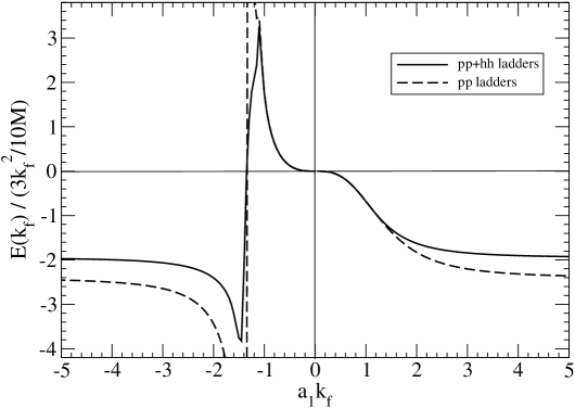
Figure 5: Energy per particle $\bar{E}(k_{f})$ from p-wave ladder diagrams divided by the free Fermi gas energy $3k_{f}^{2}/10M$ as a function of the dimensionless parameter $a_{1}k_{f}$.

It is interesting to explore the dependences on density and coupling strength of the novel p-wave resummation results eqs.(31,33). For this purpose we plot in Fig. 5 the ratio of the interaction energy $\bar{E}(k_{f})$ to the free Fermi gas energy $3k_{f}^{2}/10M$ as a function of the dimensionless parameter $a_{1}k_{f}$. The full and dashed curve correspond to the complete ladder series and partial $pp$-ladder series, respectively. On the attractive side $a_{1}k_{f}>0$ one observes that both curves stay closely together up to $a_{1}k_{f}\simeq 1.5$ and from there upwards the $pp$-ladder series develops somewhat more attraction. The behavior on the repulsive side $a_{1}k_{f}<0$ is characterized by a sharp peak of the full curve at $a_{1}k_{f}\simeq-1.1$ and an even higher peak of the dashed curve at $a_{1}k_{f}\simeq-1.3$. Beyond that a non-perturbative behavior sets in, such that both curves pass through zero at $a_{1}k_{f}\simeq-1.35$ and attraction gets generated from the repulsive scattering volume $a_{1}^{3}<0$. In order to join smoothly with the attractive side at infinity $a_{1}k_{f}=\pm\infty$, this attraction is more strongly pronounced for the $pp$-ladder series.

As a side remark we note that s-wave and p-wave contact-interactions do not interfere in the ladder diagrams. The usual argument of rotational invariance (in momentum-space) does not apply in the medium. An sp-interference term introduces into the in-medium loop a factor that is odd under parity $\vec{l}\to-\vec{l}$, but the integration regions defined by two overlapping or intersecting Fermi spheres in eqs.(5,6) are even under this transformation, and therefore it integrates always to zero.

Let us add a final remark on the physical applicability of the resummation results derived in this work. In order to obtain the factorization of multi-loop diagrams (in a generalized sense) the input interactions have to be contact-interactions. Their iteration to all orders in the vacuum leads to a unitary S-matrix with phase-shifts given by eqs.(4,26). On the other hand the Wigner bound [21] due causality states that a scattering phase-shift must not drop too fast with momentum, $\partial\delta_{l}(q)/\partial q>-\bar{R}$, where $\bar{R}$ measures the range of the interaction. In the case of (unresolved) contact-interactions the range $\bar{R}\simeq 0$ vanishes practically. This consideration could provide an argument for the condition that the resummation results are physically applicable only for positive scattering length $a>0$, positive scattering volume $a_{1}>0$, and negative effective range $r_{s}<0$.

Appendix: Resummation with coupled channels

In this appendix we supply the result for the complete resummation of in-medium ladder diagrams due to an s-wave contact-interaction in a binary (i.e. two-component) many-fermion system. The prototype of such a system is nuclear matter made up from strongly interacting protons and neutrons. Low-energy nucleon-nucleon scattering is characterized by two different scattering lengths, the spin-singlet $(I=1)$ scattering length $a_{s}\simeq 19\,$fm and the spin-triplet $(I=0)$ scattering length $a_{t}\simeq-5.4\,$fm, where $I=0,1$ denotes the total isospin. The many-body dynamics is richer and offers the possibility to introduce an isospin-asymmetry through different (variable) proton and neutron densities (or different Fermi momenta $k_{p}$ and $k_{n}$). Returning to the in-medium loop in Fig. 2 one sees that one has to deal now with four (partly coupled) states: $(pp,nn,pn,np)$. The last two channels get decoupled through a $45^{\circ}$ rotation to the isospin-eigenstates $(pn\pm np)/\sqrt{2}$. In this isospin-basis the momentum-independent contact-interaction (proportional to the scattering lengths $a_{s,t}$) is diagonal and therefore the multi-loop diagrams factorize. As a new element one encounters mixed proton-neutron loops with integration regions defined by eqs.(5,6), where one Fermi momentum $k_{f}$ is $k_{p}$ and the other is $k_{n}$. The real part of this mixed in-medium loop is given simply by the sum of two independent proton and neutron terms, but a more complicated overlap of two Fermi-spheres $|\vec{P}\pm\vec{l}\,|<k_{p,n}$ and the surface $|\vec{l}\,|=|\vec{q}\,|$ has to be evaluated for the imaginary part (see eq.(38) below). The resummation of the particle-hole ladder diagrams to all orders through an arctangent-function is also easily carried out, since for a $4\times 4$ diagonal matrix one has the identity: $\arctan({\rm diag}(d_{1},d_{2},d_{3},d_{4}))={\rm diag}(\arctan d_{1},\arctan d_{2},\arctan d_{3},\arctan d_{4})$. In order to compute the energy density one rotates back to the particle basis and adds the Hartree and Fock contributions with their spin-factors $4$ and $-2$. Putting all pieces together the final result for the energy per particle reads:

$$\bar{E}(k_{p},k_{n}) \!\!\!\!=\!\!\!\! -{24\over\pi M(k_{p}^{3}+k_{n}^{3})}\Bigg{\{}\int\limits_{0}^{1}\!ds\,s^{2}\!\!\int\limits_{0}^{\sqrt{1-s^{2}}}\!\!d\kappa\,\kappa\,\Bigg{[}k_{p}^{5}\arctan{I(s,\kappa)\over(a_{s}k_{p})^{-1}+\pi^{-1}R(s,\kappa)}$$

$$+\,k_{n}^{5}\arctan{I(s,\kappa)\over(a_{s}k_{n})^{-1}+\pi^{-1}R(s,\kappa)}\Bigg{]}+\int\limits_{0}^{(k_{p}+k_{n})/2}\!dP\,P^{2}\!\!\int\limits_{q_{\rm min}}^{q_{\rm max}}\!\!dq\,q$$

$$\times\Bigg{[}\arctan{\Phi(P,q,k_{p},k_{n})\over a_{s}^{-1}+(2\pi)^{-1}(k_{p}R_{p}+k_{n}R_{n})}+3\arctan{\Phi(P,q,k_{p},k_{n})\over a_{t}^{-1}+(2\pi)^{-1}(k_{p}R_{p}+k_{n}R_{n})}\Bigg{]}\Bigg{\}}\,,$$

with the abbreviations $R_{p}=R(P/k_{p},q/k_{p})$ and $R_{n}=R(P/k_{n},q/k_{n})$, where $R(s,\kappa)$ and $I(s,\kappa)$ are given in eqs.(16,17). The integration boundaries are:

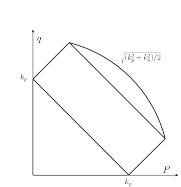
Figure 6: Support of the function $\Phi(P,q,k_{p},k_{n})$ in the $(P,q)$-plane pieced together by a triangle, a rectangle and a circular wedge. The rectangle has side-lengths $\sqrt{2}\,k_{p}$ and $(k_{n}-k_{p})/\sqrt{2}$.

$$q_{\rm min}={\rm max}\big{(}0,P-k_{p}\big{)}\,,\qquad q_{\rm max}={\rm min}\Big{(}k_{p}+P,\sqrt{(k_{n}^{2}+k_{p}^{2})/2-P^{2}}\,\Big{)}\,,$$ (37)

assuming for definiteness $k_{n}\geq k_{p}$ (i.e. an excess of neutrons over protons). The total nucleon density is $\rho=\rho_{p}+\rho_{n}=(k_{p}^{3}+k_{n}^{3})/3\pi^{2}$. The imaginary part function $\Phi(P,q,k_{p},k_{n})$ appearing in the numerator of the last two $\arctan$-terms is defined piecewise by:

$$\Phi=q\,,\,\,\,{\rm for}\,\,\,P+q<k_{p}\,,$$

$$\Phi={1\over 4P}\Big{[}k_{p}^{2}-(P-q)^{2}\Big{]}\,,\,\,\,{\rm for}\,\,\,k_{p}<P+q<k_{n}\,,\,|P-q|<k_{p}\,,$$

$$\Phi={1\over 4P}\Big{[}k_{p}^{2}+k_{n}^{2}-2(P^{2}+q^{2})\Big{]}\,,\,\,\,{\rm for}\,\,\,P+q>k_{n}\,,\,P^{2}+q^{2}<(k_{p}^{2}+k_{n}^{2})/2\,.$$ (38)

As illustrated in Fig. 6 the support of this function consists of a triangle, a rectangle and a circular wedge pieced together. Note that $P^{2}q\,\Phi(P,q,k_{p},k_{n})$ plays also the role of a weighting function (symmetric under $P\leftrightarrow q$) in reducing the integral over two Fermi spheres $|\vec{p}_{1,2}|<k_{p,n}$. The same expression for the $\Phi$-function as in eq.(38) has been derived in appendix C of ref.[14]. The numerical implications of eq.(36) for the nuclear matter equation of state are discussed elsewhere [22]. The inclusion of corrections from the singlet and triplet effective ranges should also be obvious. The inverse scattering lengths $a_{s,t}^{-1}$ in the denominators of the arctan-terms in eq.(36) get then replaced by appropriate reciprocal $\Omega$-functions. Note also the factor $3$ in front of the last arctan-term, it ensures that the result $\bar{E}(k_{f},k_{f})$ for the isospin-symmetric system, $k_{p}=k_{n}=k_{f}$, becomes invariant under the interchange ($a_{s}\leftrightarrow a_{t}$) of both scattering lengths. As a byproduct of eq.(36) we consider the isospin-asymmetry energy $A(k_{f})$. It is obtained by setting the Fermi momenta to $k_{n,p}=k_{f}(1\pm\delta)^{1/3}$ and expanding to quadratic order, $\bar{E}(k_{p},k_{n})=\bar{E}(k_{f})+\delta^{2}A(k_{f})+{\cal O}(\delta^{4})$, in the isospin-asymmetry parameter $\delta$. One finds up to second order in the scattering lengths $a_{s,t}$:

$$A(k_{f})={k_{f}^{2}\over 6M}\bigg{\{}1+{k_{f}\over\pi}(3a_{t}-a_{s})+{8k_{f}^{2}\over 5\pi^{2}}\Big{[}a_{s}^{2}(3-\ln 2)-a_{t}^{2}(2+\ln 2)\Big{]}+\dots\bigg{\}}\,,\,$$ (39)

where the first term $k_{f}^{2}/6M$ arising from the kinetic energy has been included for orientation. This result is implicitly contained in ref.[23] via the parameterizations $a_{s,t}=g_{A}^{2}M\gamma_{1,0}/(8\pi f_{\pi}^{2})$ of the scattering lengths. As a special case of an asymmetric system let us finally consider the one-component (unitary) Fermi gas in the spin-unbalanced configuration. With one singlet scattering length $a$ there is interaction taking place only in the mixed spin-state $(\uparrow\downarrow-\downarrow\uparrow)/\sqrt{2}$ and the energy per particle reads:

$$\bar{E}(k_{\uparrow},k_{\downarrow})=-{48\over\pi M(k_{\uparrow}^{3}+k_{\downarrow}^{3})}\!\!\!\!\int\limits_{0}^{(k_{\uparrow}+k_{\downarrow})/2}\!\!\!dP\,P^{2}\!\!\int\limits_{q_{\rm min}}^{q_{\rm max}}\!\!dq\,q\arctan{\Phi(P,q,k_{\uparrow},k_{\downarrow})\over a^{-1}+(2\pi)^{-1}(k_{\uparrow}R_{\uparrow}+k_{\downarrow}R_{\downarrow})}\,,$$ (40)

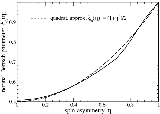
Figure 7: The (normal) Bertsch parameter $\xi_{n}(\eta)$ of the unitary Fermi gas as a function of the spin-asymmetry parameter $\eta$.

with $q_{\rm max},q_{\rm min},R_{\uparrow}$, $R_{\downarrow}$ and $\Phi(P,q,k_{\uparrow},k_{\downarrow})$ defined in complete analogy to the proton-neutron system before. Note that the density of the spin-unbalanced Fermi gas is $\rho=(k^{3}_{\uparrow}+k^{3}_{\downarrow})/6\pi^{2}$. We can use eq.(40) to determine, in the unitary limit $a\to\infty$, the dependence of the (normal) Bertsch parameter $\xi_{n}(\eta)$ on the spin-asymmetry $\eta$ of the spin-unbalanced system. Setting the Fermi momenta of the spin-up and spin-down fermions to $k_{\uparrow,\downarrow}=k_{f}(1\pm\eta)^{1/3}$, the quantity $\xi_{n}(\eta)-1$ is given by the ratio of the interaction energy $\bar{E}(k_{\uparrow},k_{\downarrow})$ to the kinetic energy $3k_{f}^{2}[(1+\eta)^{5/3}+(1-\eta)^{5/3}]/20M$. The full line in Fig. 7 shows the (normal) Bertsch parameter $\xi_{n}(\eta)$ as a function of the spin-asymmetry parameter $\eta$. The result is quite close to the parabolic approximation $\xi_{n}(\eta)=(1+\eta^{2})/2$ connecting the two boundary points $(\eta,\xi_{n})=(0,1/2)$ and $(\eta,\xi_{n})=(1,1)$.

References

- [1] Lecture Notes in Physics 836, “BCS-BEC Crossover and Unitary Fermi Gas”, W. Zwerger (editor).
- [2] M. McNeil Forbes, S. Gandolfi and A. Gezerlis, Phys. Rev. Lett. 106, 235303 (2011).
- [3] M. McNeil Forbes, S. Gandolfi and A. Gezerlis, cond-mat/1205.4815.
- [4] M.J.H. Ku, A.T. Sommer, L.W. Cheuk and M.W. Zwierlein, Nature Phys. 8, 366 (2012); cond-mat/1110.3309.
- [5] Y. Nishida and D.T. Son, Phys. Rev. Lett. 97, 050403 (2006).
- [6] S. Gandolfi et al., Phys. Rev. C79, 054005 (2009).
- [7] A. Gezerlis and J. Carlson, Phys. Rev. C81, 025803 (2011).
- [8] N. Kaiser, Nucl. Phys. A860 (2005) 41; and refs. therein.
- [9] H.W. Hammer and R.J. Furnstahl, Nucl. Phys. A678, 277 (2000).
- [10] J.V. Steele, nucl-th/0010066. The middle term in eq.(16) needs to be corrected and multiplied by a factor 2.
- [11] T. Schäfer, C.W. Kao and S.R. Cotanch, Nucl. Phys. A762 (2005) 82.
- [12] W. Zwerger, private communications.
- [13] A. Schwenk and C.J. Pethick, Phys. Rev. Lett. 95, 160401 (2005).
- [14] A. Lacour, J.A. Oller and U.G. Meißner, Ann. Phys. (NY) 326, 241 (2011); and refs. therein.
- [15] A. Gezerlis, Phys. Rev. C83, 065801 (2011).
- [16] A. Gezerlis and R. Sharma, Phys. Rev. C85, 015806 (2012).
- [17] S. Gandolfi et al., Phys. Rev. Lett. 101, 132501 (2008).
- [18] A. Akmal, V.R. Pandharipande and D.G. Ravenhall, Phys. Rev. C58, 1804 (1998).
- [19] Q. Chen et al., Phys. Rev. C77, 054002 (2006).
- [20] I. Tews, T. Krüger, K. Hebeler and A. Schwenk, nucl-th/1206.0025; and refs. therein.
- [21] H.W. Hammer and D. Lee, Ann. Phys. (NY) 325, 2212 (2010).
- [22] S. Schulteß, “Resummations and Chiral Dynamics of Nuclear Matter”, diploma thesis, TU München (2012).
- [23] S. Fritsch and N. Kaiser, Eur. Phys. J. A21, 117 (2004).