Hybrid resonance of Maxwell’s equations in slab geometry

Abstract

Hybrid resonance is a physical mechanism for the heating of a magnetic plasma. In our context hybrid resonance is a solution of the time harmonic Maxwell’s equations with smooth coefficients, where the dielectric tensor is a non diagonal hermitian matrix. The main part of this work is dedicated to the construction and analysis of a mathematical solution of the hybrid resonance with the limit absorption principle. We prove that the limit solution is singular: it consists of a Dirac mass at the origin plus a principal value and a smooth square integrable function. The formula obtained for the plasma heating is directly related to the singularity.

1 Introduction

It is known in plasma physics that Maxwell’s equation in the context of a strong background magnetic field may develop singular solutions even for smooth coefficients. This is related to what is called the hybrid resonance [13, 20, 8] for which we know no mathematical analysis. Hybrid resonance shows up in reflectometry experiments [16, 15] and heating devices in fusion plasma [19]. The energy deposit is resonant and may exceed by far the energy exchange which occurs in Landau damping [20, 27]. The starting point of the analysis is from the linearization of Vlasov-Maxwell’s equations of a non homogeneous plasma around bulk magnetic field $\mathbf{B}_{0}\neq 0$. It yields the non stationary Maxwell’s equations with a linear current

$$\left\{\begin{array}[]{ll}-\frac{1}{c^{2}}\partial_{t}\mathbf{E}+\nabla\wedge\mathbf{B}=\mu_{0}\mathbf{J},&\mathbf{J}=-eN_{e}\mathbf{u}_{e},\\ \partial_{t}\mathbf{B}+\nabla\wedge\mathbf{E}=0,\\ m_{e}\partial_{t}\mathbf{u}_{e}=-e\left(\mathbf{E}+\mathbf{u}_{e}\wedge\mathbf{B}_{0}\right)-m_{e}\nu\mathbf{u}_{e}.\end{array}\right.$$ (1.1)

The electric field is $\mathbf{E}$ and the magnetic field is $\mathbf{B}$. The modulus of the background magnetic field $|\mathbf{B}_{0}|$ and its direction $\mathbf{b}_{0}=\frac{\mathbf{B}_{0}}{|\mathbf{B}_{0}|}$ will be assumed constant in space for simplicity in our work. The absolute value of the charge of electrons is $e$, the mass of electrons is $m_{e}$, the velocity of light is $c=\sqrt{\frac{1}{\varepsilon_{0}\mu_{0}}}$ where the permittivity of vacuum is $\varepsilon_{0}$ and the permeability of vacuum is $\mu_{0}$. The third equation corresponds to moving electrons with velocity $\mathbf{u}_{e}$ where the electronic density $N_{e}$ is a given function of the space variable. One implicitly assumes an ion bath, which is the reason of the friction between the electrons and the ions with collision frequency $\nu$. Much more material about such models can be found in classical physical textbooks [20, 8]. The loss of energy in domain $\Omega$ can easily be computed in the time domain starting from (1.1). One obtains

$$\frac{d}{dt}\int_{\Omega}\left(\frac{\varepsilon_{0}\left|\mathbf{E}\right|^{2}}{2}+\frac{\left|\mathbf{B}\right|^{2}}{2\mu_{0}}+\frac{m_{e}N_{e}\left|\mathbf{u}_{e}\right|^{2}}{2}\right)=-\int_{\Omega}{\nu m_{e}N_{e}\left|\mathbf{u}_{e}\right|^{2}}+\mbox{ boundary terms}.$$

Therefore ${\cal Q}(\nu)=\int_{\Omega}{\nu m_{e}N_{e}\left|\mathbf{u}_{e}\right|^{2}}$ represents the total loss of energy of the electromagnetic field plus the electrons in function of the collision frequency $\nu$. Since the energy loss is necessarily equal to what is gained by the ions, it will be referred to as the heating. We will show that in certain conditions characteristic of the hybrid resonance in frequency domain, the heating does not vanish for vanishing collision friction. So a simple characterization of resonant heating can be written as: ${\cal Q}(0^{+})>0$. This apparent paradox is the subject of this work.

As we will prove, the mathematical solution of the time frequency formulation is not square integrable. So that, hybrid resonance is a non standard phenomenon in the context of the mathematical theory of Maxwell’s equations for which we refer to [14, 11, 26, 36]. The situation can be compared with the mathematical theory of metametarials. In [37, 38] the electric permittivity and magnetic permeability tensors are degenerate -i.e. they have zero eigenvalues- in surfaces, but they remain positive definite. In this case, the solutions are singular, but the problem remains coercive. See also [12]. In [5, 6, 4] the coefficient changes in a discontinuous way from being positive to negative. In this situation coerciveness is lost, but as the absolute value of the coefficient is bounded below by a positive constant, the solutions are regular. In our case we have both difficulties at the same time. As the coefficient $\alpha$ (see below) goes from being positive to negative in a continuous way, its absolute value is zero at a point, and, in consequence, our problem is not coercive and there are singular solutions.

1.1 Maxwell’s equations in frequency domain

We introduce the notations needed to detail the physics of the problem and to formulate our main result. Writing (1.1) in the frequency domain, that is $\partial_{t}=-i\omega$, yields

$$\left\{\begin{array}[]{ll}\frac{1}{c^{2}}i\omega\mathbf{E}+\nabla\wedge\mathbf{B}=-\mu_{0}eN_{e}\mathbf{u}_{e},\\ -i\omega\mathbf{B}+\nabla\wedge\mathbf{E}=0,\\ -im_{e}\omega\mathbf{u}_{e}=-e\left(\mathbf{E}+\mathbf{u}_{e}\wedge\mathbf{B}_{0}\right)-m_{e}\nu\mathbf{u}_{e}.\end{array}\right.$$ (1.2)

One computes the velocity using the third equation

$$\widetilde{\omega}\mathbf{u}_{e}+\omega_{c}i\mathbf{u}_{e}\wedge\mathbf{b}_{0}=-\frac{e}{m_{e}}i\mathbf{E}$$ (1.3)

where the cyclotron frequency is $\omega_{c}=\frac{e|\mathbf{B}_{0}|}{m_{e}}$, $\mathbf{b}_{0}=\frac{\mathbf{B}_{0}}{|\mathbf{B}_{0}|}$ is the normalized magnetic field and $\widetilde{\omega}=\omega+i\nu$ is the equivalent a priori complex pulsation. This is a linear equation. Assuming that $\mathbf{b}_{0}=(0,0,1)$ one gets

$$\mathbf{u}_{e}=-\frac{e}{m_{e}}i\left(\begin{array}[]{ccc}\frac{\widetilde{\omega}}{\widetilde{\omega}^{2}-\omega_{c}^{2}}&-i\frac{\omega_{c}}{\widetilde{\omega}^{2}-\omega_{c}^{2}}&0\\ i\frac{\omega_{c}}{\widetilde{\omega}^{2}-\omega_{c}^{2}}&\frac{\widetilde{\omega}}{\widetilde{\omega}^{2}-\omega_{c}^{2}}&0\\ 0&0&\frac{1}{\widetilde{\omega}}\end{array}\right)\mathbf{E}.$$ (1.4)

It is then easy to eliminate $\mathbf{u}_{e}$ from the first equation of the system (1.2) and to obtain the time harmonic Maxwell’s equation

$$\nabla\wedge\nabla\wedge\mathbf{E}-\left(\frac{\omega}{c}\right)^{2}\underline{\underline{\varepsilon}}(\nu)\mathbf{E}=0,$$ (1.5)

where $\omega$ is the frequency, $c$ the velocity of light. and the dielectric tensor is the one of the cold plasma approximation [20, 13]

$$\underline{\underline{\varepsilon}}(\nu)=\begin{pmatrix}1-\frac{\widetilde{\omega}\omega_{p}^{2}}{\omega\left(\widetilde{\omega}^{2}-\omega_{c}^{2}\right)}&i\frac{\omega_{c}\omega_{p}^{2}}{\omega\left(\widetilde{\omega}^{2}-\omega_{c}^{2}\right)}&0\\ -i\frac{\omega_{c}\omega_{p}^{2}}{\omega\left(\widetilde{\omega}^{2}-\omega_{c}^{2}\right)}&1-\frac{\widetilde{\omega}\omega_{p}^{2}}{\omega\left(\widetilde{\omega}^{2}-\omega_{c}^{2}\right)}&0\\ 0&0&1-\frac{\omega_{p}^{2}}{\omega\widetilde{\omega}}\end{pmatrix}.$$ (1.6)

The parameters of the dielectric tensor are the cyclotron frequency $\omega_{c}=\frac{e|\mathbf{B}_{0}|}{m_{e}}$ and the plasma frequency $\omega_{p}=\sqrt{\frac{e^{2}N_{e}}{\varepsilon_{0}m_{e}}}$ which depends on the electronic density $N_{e}$. We consider in this work $\omega\neq\omega_{c}$, that is the frequency is away from the cyclotron frequency, so that the dielectric tensor is a smooth bounded matrix in our work. Considering (1.3) the heating is

$${\cal Q}(\nu)=\int_{\Omega}{\nu m_{e}N_{e}\left|\mathbf{u}_{e}\right|^{2}}=-\mbox{ Re}\left(\int_{\Omega}eN_{e}\left(\mathbf{E},\mathbf{u}_{e}\right)\right).$$

One can eliminate the electron velocity in function of the electric field using (1.4) rewritten as $\mathbf{u}_{e}=-\frac{e}{m_{e}}i\frac{\omega}{\omega_{p}^{2}}\left(\mathbf{I}-\underline{\underline{\varepsilon}}(\nu)\right)\mathbf{E}$. Therefore a third formula is

$${\cal Q}(\nu)={\omega\varepsilon_{0}}\mbox{ Im}\left(\int_{\Omega}\left(\mathbf{E},\underline{\underline{\varepsilon}}(\nu)\mathbf{E}\right)\right)$$ (1.7)

where $\underline{\underline{\varepsilon}}(\nu)$ is the dielectric tensor (1.6).

A discussion of the heating in the limit of small collision frequency establishes the physical basis of the limit absorption principle that will be used in this work. Indeed physical values in fusion plasmas are such that the collision frequency is much smaller than the frequency ($\nu<<\omega$) which means that some simplifications can be done in the dielectric tensor, as in [20] page 197. The limit tensor for $\nu=0$ is

$$\underline{\underline{\varepsilon}}(0)=\begin{pmatrix}1-\frac{\omega_{p}^{2}}{\omega^{2}-\omega_{c}^{2}}&i\frac{\omega_{c}\omega_{p}^{2}}{\omega\left(\omega^{2}-\omega_{c}^{2}\right)}&0\\ -i\frac{\omega_{c}\omega_{p}^{2}}{\omega\left(\omega^{2}-\omega_{c}^{2}\right)}&1-\frac{\omega_{p}^{2}}{\omega^{2}-\omega_{c}^{2}}&0\\ 0&0&1-\frac{\omega_{p}^{2}}{\omega^{2}}\end{pmatrix}.$$ (1.8)

We notice that $\underline{\underline{\varepsilon}}(0)=\underline{\underline{\varepsilon}}(0)^{*}$ is an hermitian matrix, so $\underline{\underline{\varepsilon}}(0)$ cannot be used alone to obtain a consistent evaluation of the heating. Linearization of the dielectric tensor yields $\underline{\underline{\varepsilon}}(\nu)=\underline{\underline{\varepsilon}}(0)+\nu\underline{\underline{\varepsilon}}^{\prime}(0)+O(\nu^{2})$ with $\underline{\underline{\varepsilon}}^{\prime}(0)=i\left(\begin{array}[]{ccc}\lambda_{1}&-i\lambda_{2}&0\\ i\lambda_{2}&\lambda_{1}&0\\ 0&0&\lambda_{3}\end{array}\right)$ where $\lambda_{1}=\frac{\omega_{p}^{2}\left(\omega^{2}+\omega_{c}^{2}\right)}{\omega\left(\omega^{2}-\omega_{c}^{2}\right)^{2}}$, $\lambda_{2}=\frac{2\omega_{c}\omega_{p}^{2}}{\left(\omega^{2}-\omega_{c}^{2}\right)^{2}}$ and $\lambda_{3}=\frac{\omega_{p}^{2}}{\omega^{3}}$. Since $\lambda_{1}^{2}\geq\lambda_{2}^{2}$, one gets that $-i\underline{\underline{\varepsilon}}^{\prime}(0)$ is a symetric non negative matrix. This correction term is the one that generates the heating in (1.7). In the sequel we will consider the simplified linear approximation

$$\underline{\underline{\varepsilon}}(\nu)=\underline{\underline{\varepsilon}}(0)+i\nu\mathbf{I},$$ (1.9)

yielding the physical basis of the limit absorption principle.

1.2 X-mode equations in slab geometry

The hybrid resonance concerns more specifically the $2\times 2$ upper-left block in (1.8), which corresponds to the transverse electric (TE) mode, $E=(E_{x},E_{y},0)$, and $E_{x},E_{y}$, independent of $z$. In the limit case $\nu=0$, one gets the system

$$\left\{\begin{array}[]{rrrr}W&+\partial_{y}E_{x}&-\partial_{x}E_{y}&=0,\\ \partial_{y}W&-\alpha E_{x}&-i\delta E_{y}&=0,\\ -\partial_{x}W&+i\delta E_{x}&-\alpha E_{y}&=0,\end{array}\right.$$ (1.10)

where $W$ and the magnetic field $B_{z}$ are proportional. The coefficients are

$$\alpha=\frac{\omega^{2}}{c^{2}}\left(1-\frac{\omega_{p}^{2}}{\omega^{2}-\omega_{c}^{2}}\right)\qquad\delta=\frac{\omega^{2}}{c^{2}}\times\frac{\omega_{c}\omega_{p}^{2}}{\omega\left(\omega^{2}-\omega_{c}^{2}\right)}.$$ (1.11)

Simplified coefficients in slab geometry will be defined below.

Figure 1: X-mode in slab geometry: the domain. In a real physical device an antenna is on the wall on the left and sends an incident electromagnetic wave through a medium which is assumed infinite for simplicity. The incident wave generates a reflected wave. We will characterize the antenna by the knowledge of the non homogeneous boundary condition (1.12). The medium is filled with a plasma with dielectric tensor given by (1.8).

Figure 2: X-mode equations in slab geometry: the physical parameters. The electronic density $x\mapsto N_{e}(x)$ is low at the boundary, and increases towards a plateau. The background magnetic field $B_{0}$ is taken as constant for simplicity.

In the plasma community this system is referred to as the X-mode equations, where the letter X stands for eXtraordinary mode or eXtraordinary waves. We suspect the reason is the non standard behavior of the solutions of this system. The case where $\omega=\omega_{c}$, i.e., when the frequency of the incident wave, $\omega$, is equal to the cyclotron frequency, $\omega_{c}$, will not be considered in this work. That is we consider that $\omega\neq\omega_{c}$. If $\omega<\omega_{c}$ it is called a low hybrid resonance. The other case $\omega>\omega_{c}$ is denoted as the upper hybrid resonance. On the other hand we will assume that the diagonal coefficient $\alpha$ is smooth and vanishes at $x=0$. This configuration corresponds to the hybrid resonance.

To be more specific we consider the simplified 2D domain

$$\Omega=\left\{(x,y)\in\mathbb{R}^{2},\quad-L\leq x,\quad y\in\mathbb{R},\quad L>0\right\}.$$

Boundary conditions for the Maxwell’s equations can be of usual types, that is metallic condition $n\wedge E=0$, non homogeneous absorbing boundary condition like $curlE+i\lambda n\wedge E=g$ on some parts of the boundary or even natural absorbing boundary condition at infinity. Concerning the X-mode equations (1.10) we consider a non homogeneous boundary condition

$$W+i\lambda n_{x}E_{y}=g\mbox{ on the left boundary }x=-L,\qquad\lambda>0,$$ (1.12)

which models a given source, typically a radiating antenna. In real Tokamaks this antenna is used to heat or to probe the plasma. Such devices are actually being studied for the purposes of reflectometry and heating of magnetic fusion plasmas in the context of the international ITER project: the ITER project is about the design of new Tokamak with enhanced fusion capabilities [25].

1.3 Coefficients in slab geometry

We consider slab geometry. That is all coefficients $\alpha$ and $\delta$ are functions only of the variable $x$: $\partial_{y}\alpha=\partial_{y}\delta=0$. The main physical hypothesis is that the extra-diagonal part of the dielectric tensor is dominant at a finite number of points, that is

$$\alpha(x_{i})=0,\;\alpha^{\prime}(x_{i})\neq 0\mbox{ and }\delta(x_{i})\neq 0,\quad x_{i}\in\mathbb{R},\;i=1,\dots,N.$$

To fix the notations we add other mathematical assumptions which are reasonable in the physical context of idealized reflectometry or heating devices. We suppose that $N=1$ and $x_{1}=0$. We will use

$$\delta\in{\cal C}^{1}[-L,\infty[,\qquad\delta(0)\neq 0,$$ (1.13)

$$\alpha\in{\cal C}^{2}[-L,\infty[,\qquad\alpha(0)=0,\quad\alpha^{\prime}(0)<0.$$ (H1)

Moreover

$$\alpha_{-}\leq\alpha(x)\leq\alpha_{+},\;\forall x\in[-L,\infty[,\qquad\mbox{ and }\;\;0<r\leq\left|\frac{\alpha(x)}{x}\right|,\;\forall x\in[-L,H]$$ (H2)

where $H>0$.

Figure 3: X-mode equations in slab geometry: parameters of the dielectric tensor deduced from the value of the physical parameters described in figure 2, assuming that $\omega>\omega_{c}$. The coefficient $\alpha$ decreases from positive to negative values. It crosses the axis with a slope bounded from below by $r$. The coefficient $\delta$ is positive and bounded. Since the electromagnetic wave is strongly absorbed for $x\geq H$, we simplify by taking all coefficients constant for $x\geq H$ because it does not change the physics of the problem.

We will also assume that the coefficients are constant at large scale: there exists $\delta_{\infty}$ and $\alpha_{\infty}$ so that

$$\delta(x)=\delta_{\infty}\mbox{ and }\alpha(x)=\alpha_{\infty}\qquad H\leq x<\infty.$$ (H3)

Therefore $\alpha,\delta\in L^{\infty}(-L,\infty)$. We also assume the problem is coercive at infinity,

$$\alpha_{\infty}^{2}-\delta^{2}_{\infty}>0.$$ (H4)

An additional condition is defined by

$$4\|\delta\|_{\infty}^{2}H<r.$$ (H5)

It expresses the fact that the length of the transition zone between $x=0$ and $x=H$ is small with respect to the other parameters of the problem. One can refer to Figures 2 and 3 for a graphical representation. This hypothesis is physically very reasonable. It is known in the physical community that this problem may be highly singular at the origin. With these hypotheses, one can consider as well other coefficients are now normalized $\omega=c=\varepsilon_{0}=\mu_{0}=1$. As explained previously in (1.9), the solutions in the context of the limit absorption principle correspond to adding a complex part to the diagonal coefficient $\alpha$, that is $\alpha$ is replaced by $\alpha+i\nu$.

1.4 Main result

Our main result can be summarized as follows. Following the convention introduced in $(7.1.3)$ from [17], we denote by $\widehat{g}$ the Fourier transform of $g$,

$$\widehat{g}(\theta):=\int_{\mathbb{R}}\,g(y)\,e^{-i\theta y}\,dy.$$

We need the uniform transversality assumption (H6) which is a generalization of assumption (H5). See Section 7.

Theorem 1.1.

Assuming (H1-H6) and $g\in L^{2}(\mathbb{R})$ with $\widehat{g}$ of compact support, there exists a solution of (1.10) with boundary condition (1.12) that goes to zero at infinity. This solution is in the sense of distributions and is constructed with the limit absorption principle by taking the limit $\nu=0^{+}$ in (7.4).

A representation formula is

$$\left(\begin{array}[]{c}E_{x}^{+}\\ E_{y}^{+}\\ W^{+}\end{array}\right)(x,y)=\frac{1}{2\pi}\int_{\mathbb{R}}\frac{\widehat{g}(\theta)}{\tau^{\theta,+}}\left(\begin{array}[]{c}P.V.\frac{1}{\alpha(x)}+\frac{i\pi}{\alpha^{\prime}(0)}\delta_{D}+u_{2}^{\theta,+}\\ v_{2}^{\theta,+}\\ w_{2}^{\theta,+}\end{array}\right)e^{i\theta y}d\theta.$$ (1.14)

This formula depends on a certain transfer coefficient $\tau^{\theta,+}$ defined in (7.3), and on three $L^{2}$ functions $(u_{2}^{\theta,+},v_{2}^{\theta,+},w_{2}^{\theta,+})$ defined in Theorem 5.2. Unless the source term $g$ is identically zero, the electric field $E_{x}$ does not belong to $L^{1}_{{\rm loc}}\left((-L,\infty)\times\mathbb{R}\right)$. The other components are always more regular: in particular $E_{y}^{+},W^{+}\in L^{2}\left((-L,\infty)\times\mathbb{R}\right)$.

The value of the resonant heating is

$${\cal Q}^{+}=\frac{1}{2}\int_{\mathbb{R}}\frac{\left|\widehat{g}(\theta)\right|^{2}}{\left|\alpha^{\prime}(0)\right|\left|\tau^{\theta,+}\right|^{2}}d\theta>0.$$ (1.15)

Remark 1.

An essential consequence of this analysis is the resonant heating ${\cal Q}^{+}$ which is directly related to the singularity $P.V.\frac{1}{\alpha(x)}+\frac{i\pi}{\alpha^{\prime}(0)}\delta_{D}$ of the mathematical solution $E_{x}$. The singularity is not an artifact of the model. It is on the contrary a direct way to measure the amount of heating provided to the ions by the electromagnetic wave. Concerning $E_{y}$ and $B_{z}$ which are integrable, a logarithmic divergence is still present in the solution as seen in the solution (2.2) of the Budden problem, or also in (5.57-5.58) for example.

Remark 2.

The hypothesis $\delta(0)\neq 0$ is technically important in our work. It is used two times: in the solution of the Budden problem (2.1) and in the normalization (5.15) of the singular solution since we divide by $\delta(0)$.

To our knowledge this is the first time that such formulas are written where all terms are explicitly given. A similar but much less precise formula can be found in [13] derived by means of analogies, see also [30]. The formulas (1.14-1.15) have been confirmed by numerical simulations [24] where additional information may be found about the the case where (H5,H6) are not satisfied. It must be mentioned that the numerical tests show a fast pointwise convergence of the numerical solution to the exact one, except at the origin of course. Moreover our numerical tests show that a large part of the incoming energy of the wave may be absorbed by the heating, around 90% in some cases. This is for example the case for the Fourier mode $\theta=0$ with $L=2$: the physical coefficients in (1.11) are $c=\omega=2$ and $\omega_{c}=1$, so that $\alpha=1-2\delta$. We consider the profiles

$$\alpha(x)=\left\{\begin{array}[]{lc}1,&-L\leq x\leq-1,\\ -x,&-1\leq x\leq 3,\\ -3,&3\leq x<\infty,\end{array}\right.\mbox{ and }\delta(x)=\left\{\begin{array}[]{lc}0,&-L\leq x\leq-1,\\ \frac{x+1}{2},&-1\leq x\leq 3,\\ 2,&3\leq x<\infty,\end{array}\right.$$

which satisfy additionally $|\alpha_{\infty}|>|\delta_{\infty}|$ and the fact that the electronic density is increasing from the left to the right. For the calculation of the heating we use equation (5.14) with $M=-L$ , $N=\infty$, and we observe that for normal incidence $W_{2}^{0,0}=\frac{d}{dx}V_{2}^{0,0}$ and that for $-L\leq x\leq-1$, $V_{2}^{0,0}$ is a linear combination of an incoming plane wave and a reflected plane wave. Furthermore, we compute numerically the singular solution $\mathbf{U}_{2}^{0,\nu}$ taking $\nu=10^{-3}$ as a small regularization parameter. The efficiency of the heating is defined as the ratio of the heating $\cal Q$ over the incoming energy. In this case our calculations show an efficieny of around $95\%$. Another calculation in oblique incidence $\theta=\cos\frac{\pi}{4}$ shows an efficiency still around $76,7\%$. These values indicate a high efficiency.

The method of the proof is based on an original singular integral equation attached to the Fourier solution. Introduced in the seminal work of Hilbert [23] and Picard [29], this type of integral equation is referred to as integral equation of the third kind, by comparison with the more classical equations of the first and second kind. Some references about this type of equations may be found in [3, 32] for mathematical analysis, and [34, 10, 21] for relation with theory of particles or plasma physics. Our results are therefore reminiscent of those of Bart and Warnock [3], even if our kernel does not satisfy exactly their hypothesis since it is less regular: that is the solution is the sum of a Dirac mass plus a principal value (plus a regular part). In their work it is stressed that non uniqueness is the rule for such equations. In our case, we are able to obtain uniqueness by means of the limit absorption principle which is a physically based selection principle. One originality of this work is the analysis of the properties of this singular equation for which we found no equivalent in the classical literature [1, 2, 7]. The result will be obtained with the limit absorption principle combined with a specific original integral representation of the solution. The loss of regularity of the electric field is counter intuitive with respect to the standard theory of existence and uniqueness for solutions of time harmonic Maxwell’s equations [14, 11, 26, 36]. The essential part of the proof consists in showing that the Fourier transform $\widehat{E}_{x}$ may be composed of three contributions: a Dirac mass at $x=0$; a non integrable function proportional to $\frac{1}{\alpha(x)}$, that is interpreted as a distribution in the sense of principal value; and a regular part. The condition $\alpha^{\prime}(0)<0$ guarantees that the coefficient in front of the Dirac mass is finite. Moreover, the condition (H5) simplifies some parts of the mathematical analysis. The solution is a priori non unique since the limit absorption principle generates two solutions depending on the sign of the regularization. The heating of the plasma (1.15) is directly related to the singular part of the solution.

1.5 Organization

This work is organized as follows. Section 2 is devoted to basic considerations. In the next section we introduce a regularization parameter, and we propose a specific integral representation of the solution. After that we recall the Plemelj-Privalov theorem and explain why it cannot be used directly for our problem. Section 5 is where we prove the properties of the solutions of the regularized equations. In particular, we show that one basis function has a fundamental singularity. Next, in Section 6 we define the limit spaces. The main theorem is finally proved in section 7.

2 Basic considerations

In this section we rederive the phase velocity, compute the analytic solutions of the simplified Budden problem and introduce the limit absorption principle.

2.1 Phase velocity

Recall that the phase velocity measures the velocity of individual Fourier modes.

2.1.1 Constant coefficients

Let us consider first that $\alpha$ and $\delta$ are constant at least locally. A plane wave $(E_{x},E_{y})=Re^{i(k_{1}x+k_{2}y)}$, $R\in\mathbb{C}^{2}$, is solution of X-mode equations (1.10) if and only if

$$\left[\left(\begin{array}[]{cc}k_{2}^{2}&-k_{1}\,k_{2}\\ -k_{1}\,k_{2}&k_{1}^{2}\end{array}\right)-\frac{\omega^{2}}{c^{2}}\left(\begin{array}[]{cc}\alpha&i\delta\\ -i\delta&\alpha\end{array}\right)\right]R=0,\qquad k=(k_{1},k_{2})\in\mathbb{R}^{2}.$$

We assume that $c=1$ for simplicity. We set $k=|k|d$ with $d=(\cos\theta,\sin\theta)$ the direction of the wave. The phase velocity $v_{\varphi}=\frac{\omega}{|k|}$ is solution of the eigenvalue problem

$$\left(\begin{array}[]{cc}\sin\theta^{2}-v_{\varphi}^{2}\alpha&-\cos\theta\sin\theta-iv_{\varphi}^{2}\delta\\ -\cos\theta\sin\theta+iv_{\varphi}^{2}\delta&\cos\theta^{2}-v_{\varphi}^{2}\alpha\end{array}\right)R=0.$$

The determinant of the matrix is $D=v_{\varphi}^{4}\left(\alpha^{2}-\delta^{2}\right)-v_{\varphi}^{2}\alpha$. Setting $D=0$ we obtain the phase velocity: $v_{\varphi}^{2}=\frac{\alpha}{\alpha^{2}-\delta^{2}}$.

2.1.2 Non constant coefficients

Let us assume for example that $\alpha=-x$ and that $\delta=1$ which is locally compatible with the general assumptions of Figure 3. We plot in Figure 4 the phase velocity as a function of the horizontal space coordinate. When the phase velocity is real we are in a propagating region, and when the phase velocity is pure imaginary we are in a non-propagating region. One distinguishes two cutoffs where the local phase velocity is infinite

$$\mbox{Cutoff}:\quad\alpha(x)=\pm\delta(x)$$

and one resonance where the phase velocity is null

$$\mbox{Resonance}:\alpha(x)=0.$$

This structure is characteristic of the hybrid resonance.

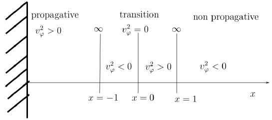
Figure 4: Sign of the square of the phase velocity $v_{\varphi}^{2}=\frac{x}{1-x^{2}}$, for $\alpha=-x$ and $\delta=1$.

Remark 3.

In what follows we always take $\omega=c=\varepsilon_{0}=\mu_{0}=1$.

2.2 The Budden problem

In the case where the solution is independent of $y$, what for the plane waves corresponds to normal incidence, that is $\theta=0$, the system (1.10) is called the Budden problem [13]

$$\left\{\begin{array}[]{lr}W-E_{y}^{\prime}&=0,\\ -\alpha E_{x}-i\delta E_{y}&=0,\\ -W^{\prime}+i\delta E_{x}-\alpha E_{y}&=0.\end{array}\right.$$

After elimination of $E_{x}$ and $W$ we obtain that,

$$-E_{y}^{\prime\prime}+\left(\frac{\delta^{2}}{\alpha}-\alpha\right)E_{y}=0$$

This equation can be solved analytically in some cases which helps a lot to understand the singularity of the general problem. Let us consider that $\alpha=-x$ and $\delta$ is solution of $\frac{\delta^{2}}{x}-x=-\frac{1}{4}+\frac{1}{x}$. The positive solution is $\delta(x)=\sqrt{x^{2}-\frac{x}{4}+1}>0$. The y-component of the electric field is solution of

$$E_{y}^{\prime\prime}+\left(-\frac{1}{4}+\frac{1}{x}\right)E_{y}=0.$$ (2.1)

This equation is of Whittaker type [1, 2]. It is a particular case of the confluent hypergeometric equation, and can also be rewritten under the Kummer form. The general theory shows that the first fundamental solution is regular

$$v(x)=e^{-\frac{x}{2}}x$$

Indeed $v^{\prime}(x)=e^{-\frac{x}{2}}\left(1-\frac{x}{2}\right)$ and $v^{\prime\prime}(x)=e^{-\frac{x}{2}}\left(-1+\frac{x}{4}\right)$, so that $v^{\prime\prime}+\left(-\frac{1}{4}+\frac{1}{x}\right)v=0$. Let us consider a second solution $w$ with linear independence with respect to the first one. The linear independence can be characterized by the normalized Wronskian relation $v(x)w^{\prime}(x)-v^{\prime}(x)w(x)=1$. Seeking for a representation $w=vz$, one gets that

$$v^{2}z^{\prime}=1\Rightarrow z=\int\frac{dx}{v^{2}}\Rightarrow w=v\int\frac{dx}{v^{2}}=x\,e^{-x/2}\,\int\frac{e^{x}}{x^{2}}.$$

Moreover, from formulas $8.212$ of [22],

$$\int\frac{e^{x}}{x^{2}}=-\frac{e^{x}}{x}+\int\frac{e^{x}}{x}=-\frac{e^{x}}{x}+E_{i}(x),$$

where $E_{i}(x)$ is the Exponential-integral function. It follows that $w(x)=-e^{x/2}+x\,e^{-x/2}\,E_{i}(x)$. Furthermore from formulas $8.214$ of [22]

$$E_{i}(x)=C+\ln|x|+\sum_{j=1}^{\infty}\frac{x^{j}}{j\cdot j!}.$$

It follows that,

$$w(x)=-1+Cx+x\,\ln|x|+O(|x|),\quad|x|\rightarrow 0.$$ (2.2)

We notice that the second function $w$ is bounded, but non regular at origin. It shows the subtleties associated with the singular Whittaker equation (2.1). Nevertheless we note that the general form of the $y$ component of the electric field of the Budden problem is bounded

$$E_{y}=av+bw\Rightarrow E_{y}\in L^{\infty}(]-\epsilon,\epsilon[).$$

The $x$ component of the electric field is more singular. It is a linear combination of two functions, the first one which is regular and bounded

$$E_{x}^{v}(x)=i\frac{\sqrt{x^{2}-\frac{x}{4}+1}}{x}v(x)=ie^{-\frac{x}{2}}\sqrt{x^{2}-\frac{x}{4}+1},$$

and the second one which is singular at origin since $w(0)=-1$

$$E_{x}^{w}(x)=i\frac{\sqrt{x^{2}-\frac{x}{4}+1}}{x}w(x).$$

The general form of the $x$ component of the electric field is a linear combination of these two functions. Since $E_{x}^{w}\not\in L^{2}(]-\epsilon,\epsilon[)$, we notice that the electric field is not a square integrable function in general.

2.3 Limit absorption principle

We will develop a regularized approach to give a rigorous meaning to the solution at all incidences. This regularized approach is based on the limit absorption principle. One considers a parameter $\nu\neq 0$ (the precise sign will be justified later) and the regularized problem with unknown $(E_{x}^{\nu},E_{y}^{\nu},W^{\nu})$

$$\left\{\begin{array}[]{cccr}W^{\nu}&+\partial_{y}E_{x}^{\nu}&-\partial_{x}E_{y}^{\nu}&=0,\\ \partial_{y}W^{\nu}&-(\alpha(x)+i\nu)E_{x}^{\nu}&-i\delta(x)E_{y}^{\nu}&=0,\\ -\partial_{x}W^{\nu}&+i\delta(x)E_{x}^{\nu}&-(\alpha(x)+i\nu)E_{y}^{\nu}&=0.\end{array}\right.$$ (2.3)

The regularization parameter $\nu$ can be interpreted as a small collision frequency.

A further simplification consists in Fourier reduction. Since the coefficients do not depend on the $y$ variable, one can perform the usual one dimension reduction. The system that will be studied in this article is obtained by applying the Fourier transform to the regularized system (2.3). Denoting the unknowns $(U,V,W)$ it yields

$$\left\{\begin{array}[]{cccr}W&+i\theta U&-V^{\prime}&=0,\\ i\theta W&-(\alpha(x)+i\nu)U&-i\delta(x)V&=0,\\ -W^{\prime}&+i\delta(x)U&-(\alpha(x)+i\nu)V&=0.\end{array}\right.$$ (2.4)

Here the notation ^′ denotes the derivative with respect to the $x$ variable.

3 A general integral representation

We begin by some notations. Let us denote by $(A_{\nu},B_{\nu})$ the two fundamental solutions of the modified equation

$$-u^{\prime\prime}-(\alpha(x)+i\nu)u=0,$$ (3.1)

with the usual normalization

$$A_{\nu}(0)=1,\quad A_{\nu}^{\prime}(0)=0\qquad\mbox{ and }B_{\nu}(0)=0,\quad B_{\nu}^{\prime}(0)=1.$$ (3.2)

Various usual continuity estimates of $A_{\nu}$ and $B_{\nu}$ can be derived: we refer for example for the appendix of [18]. Let us denote $\mathcal{D}_{z}^{\theta}$ the operator $i\theta\partial_{z}-i\delta(z)$ applied to any function $h$, that is

$$\mathcal{D}_{z}^{\theta}h=i\theta\partial_{z}h-i\delta(z)h.$$ (3.3)

Let us define the kernel

$$k^{\nu}(x,z)=B_{\nu}(z)A_{\nu}(x)-B_{\nu}(x)A_{\nu}(z).$$ (3.4)

Next we define

$$K_{1}^{\theta,\nu}(x,z;G)=\left\{\begin{array}[]{lll}\displaystyle\frac{\mathcal{D}_{x}^{\theta}\mathcal{D}_{z}^{\theta}k^{\nu}(x,z)}{\alpha(x)+i\nu},&\mbox{ for }G\leq z\leq x&\mbox{ or }x\leq z\leq G,\\ 0,&\mbox{ in all other cases}.\end{array}\right.$$ (3.5)

Let us define the kernel sequence by

$$K_{n+1}^{\theta,\nu}(x,z;G)=\int_{G}^{x}\frac{\mathcal{D}_{x}^{\theta}\mathcal{D}_{z}^{\theta}k^{\nu}(x,t)}{\alpha(x)+i\nu}K_{n}^{\theta,\nu}(t,z;G)dt.$$ (3.6)

The sum is

$$\mathcal{K}^{\theta,\nu}(x,z;G)=\sum_{n=0}^{\infty}K_{n+1}^{\theta,\nu}(x,z;G).$$ (3.7)

The integration domain is centered on $G$, that is

$$\mbox{supp}\left(K_{1}^{\theta,\nu}(\cdot,\cdot;G)\right)\subset\left\{(x,y)\in\mathbb{R}^{2};\quad G\leq z\leq x\mbox{ or }x\leq z\leq G\right\}\equiv{\cal D}_{G},$$ (3.8)

which yields as well: $\mbox{supp}\left(\mathcal{K}^{\theta,\nu}(\cdot,\cdot;G)\right)\subset{\cal D}_{G}$.

Proposition 3.1.

Any triplet $(U,V,W)$ solution of the regularized system (2.4) admits the following integral representation.

• One first chooses an arbitrary reference point $G\in[-L,\infty[$.

• The $x$ component of the electric field is solution of the integral equation

  $$U(x)-\int_{G}^{x}\frac{\mathcal{D}_{x}^{\theta}\mathcal{D}_{z}^{\theta}k^{\nu}(x,z)}{\alpha(x)+i\nu}U(z)dz=\frac{F^{\theta,\nu}(x)}{\alpha(x)+i\nu},$$ (3.9)

  where the right hand side is

  $${F^{\theta,\nu}(x)}=a_{G}\mathcal{D}_{x}^{\theta}A_{\nu}(x)+b_{G}\mathcal{D}_{x}^{\theta}B_{\nu}(x)$$ (3.10)

  and the kernel is given in (3.3-3.4). The solution of this integral equation is naturally provided by the resolvent integral formula

  $$U(x)=\frac{F^{\theta,\nu}(x)}{\alpha(x)+i\nu}+\int_{G}^{x}\mathcal{K}^{\theta,\nu}(x,z;G)\frac{F^{\theta,\nu}_{G}(z)}{\alpha(z)+i\nu}dz$$ (3.11)

  where the resolvent kernel is constructed in (3.7).

• The $y$ component of the electric field is recovered as

  $$V(x)=a_{G}A_{\nu}(x)+b_{G}B_{\nu}(x)+\int_{G}^{x}\mathcal{D}_{z}^{\theta}k^{\nu}(x,z)U(z)dz,$$ (3.12)

  and the vorticity is recovered as

  $$W(x)=a_{G}A_{\nu}^{\prime}(x)+b_{G}B_{\nu}^{\prime}(x)+\int_{G}^{x}\partial_{x}\mathcal{D}_{z}^{\theta}k^{\nu}(x,z)U(z)dz.$$ (3.13)

• The two complex numbers $(a_{G},b_{G})$ solve the linear system

  $$\left\{\begin{array}[]{ll}a_{G}A_{\nu}(G)+b_{G}B_{\nu}(G)=V(G),\\ a_{G}A_{\nu}^{\prime}(G)+b_{G}B_{\nu}^{\prime}(G)=W(G).\end{array}\right.$$ (3.14)

Proof.

Eliminating $W$ from the first and third equations of (2.4) gives

$$-V^{\prime\prime}-(\alpha+i\nu)V=f\qquad\mbox{ with }f=-i\theta U^{\prime}-i\delta U.$$

Since the Wronskian is constant, it follows from the normalization (3.2) that $A_{\nu}B_{\nu}^{\prime}-A_{\nu}^{\prime}B_{\nu}=1$. Then, from the variation of constants formula,

$$V(x)=a_{f}A_{\nu}(x)+b_{f}B_{\nu}(x)+\int_{G}^{x}f(z)k^{\nu}(x,z)dz,\quad\forall x.$$ (3.15)

where $a_{f}$ and $b_{f}$ are two integration constants. Now we replace $f$ by the corresponding function of $U$ and perform the integration by part

$$\int_{G}^{x}U^{\prime}(z)k^{\nu}(x,z)dz=U(x)k^{\nu}(x,x)-U(G)k^{\nu}(x,G)-\int_{G}^{x}U(z)\partial_{z}k^{\nu}(x,z)dz.$$

Since $k^{\nu}(x,x)=0$ there is a simplification. Therefore (3.15) yields (3.12) with $a_{G}=a_{f}+i\theta U(G)B_{\nu}(G)$ and $b_{G}=b_{f}-i\theta U(G)A_{\nu}(G)$. Next we eliminate $W$ from the first and second equations of (2.4) and obtain

$$-i\theta V^{\prime}-\theta^{2}U+(\alpha+i\nu)U+i\delta V=0.$$ (3.16)

The derivative of (3.12) yields

$$V^{\prime}(x)=a_{G}A_{\nu}^{\prime}(x)+b_{G}B_{\nu}^{\prime}(x)+\int_{G}^{x}\partial_{x}\mathcal{D}_{z}^{\theta}k^{\nu}(x,z)U(z)dz+\mathcal{D}_{z}^{\theta}k^{\nu}(x,x)U(x).$$

Since $\mathcal{D}_{z}^{\theta}k^{\nu}(x,x)=i\theta\left(A_{\nu}B_{\nu}^{\prime}-B_{\nu}A_{\nu}^{\prime}\right)=i\theta$, one gets the identity

$$V^{\prime}(x)=a_{G}A_{\nu}^{\prime}(x)+b_{G}B_{\nu}^{\prime}(x)+\int_{G}^{x}\partial_{x}\mathcal{D}_{z}^{\theta}k^{\nu}(x,z)U(z)dz+i\theta U(x).$$

Plugging this expression in (3.16) and performing all simplifications we obtain the integral equation (3.9). Finally, we get the last integral formula (3.13) from $W=-i\theta U+V^{\prime}$. The linear system (3.14) is obvious from (3.12-3.13) at $x=G$. ∎

Following [29], the equation (3.9) is an integral equation of the third kind in the case $\nu=0$. In this case the theory is rather incomplete regarding existence and uniqueness [3]. However as long as $\nu\neq 0$, the solution based on these integral equations is uniquely defined. Then, the question is to determine the behavior of these solutions when $\nu$ goes to $0$. Moreover, different choices of $G$ will give different kind of information. A strategy to study of the limit solution $\nu\rightarrow 0$ can be the following: Choose an optimal $G$, so that a) the integration constants $(a_{G},b_{G})$ are easy to determine, and b) the resolvent kernel ${\cal K}^{\theta,\nu}(\cdot,\cdot;G)$ admits a limit as $\nu\rightarrow 0$. Considering the form of the right hand side in (3.11), a convenient tool is the Plemelj-Privalov Theorem [28, 31]. Unfortunately, we will see that a fundamental singularity of the kernel ${\cal K}^{\theta,\nu}(\cdot,\cdot;G)$ prevents any simple limit procedure. A more convenient technique will be proposed in Section 5.

4 Singularity of the kernels

A fundamental tool in order to pass to the limit in singular integrals is the Plemelj-Privalov theorem [28, 31]. However, to apply this theorem to pass to the limit $\nu\rightarrow 0$ in equation (3.11) it is necessary that the kernel $\mathcal{K}^{\theta,\nu}(x,z)$ be a Hölder continuous function of $z$ for each fixed $x$. Unfortunately, this regularity is not available in our case. To illustrate this phenomenon, we study only the first term of the series (3.6) that defines $\mathcal{K}^{\theta,\nu}$, namely

$$\mathcal{K}^{\theta,\nu}_{1}(x,z):=\frac{\mathcal{D}_{x}^{\theta}\mathcal{D}_{z}^{\theta}k^{\nu}(x,z)}{\alpha(x)+i\nu}.$$ (4.1)

We consider two cases.

4.1 First case: $G\neq 0$

In this case there exists $(0,z)\in\mathcal{D}_{G}$ with $z\neq 0$. In the limit case $\nu=0$ one has that $\mathcal{K}^{\theta,0}_{1}(x,z)$ admits the local expansion:

$$\mathcal{K}^{\theta,0}_{1}(x,z)\approx\frac{1}{x\,\,\alpha^{\prime}(0)}\,\mathcal{D}^{\theta}_{x}\,\mathcal{D}^{\theta}_{z}\,k^{0}(x,z).$$

Therefore, $\mathcal{K}^{\theta,0}_{1}(x,z)$ blows up as $x\rightarrow 0$.

4.2 Second case: $G=0$

We turn to the case $G=0$. We begin with a preliminary result.

Proposition 4.1.

One has

$$(\mathcal{D}_{x}^{\theta}\mathcal{D}_{z}^{\theta}k^{\nu})(x,x)=0\quad\forall x\in\mathbb{R}.$$ (4.2)

Proof.

Indeed by construction

$$(\mathcal{D}_{x}^{\theta}\mathcal{D}_{z}^{\theta}k^{\nu})(x,x)=-\delta(x)\delta(x)k^{\nu}(x,x)$$

$$+\theta\,\delta(x)\left((\partial_{x}k^{\nu})(x,x)+(\partial_{z}k^{\nu})(x,x)\right)-\theta^{2}(\partial_{x}\partial_{z}k^{\nu})(x,x).$$

We notice that by definition $k_{\nu}(x,x)=0$ for all $x$ so the first contribution vanishes in $(\mathcal{D}_{x}^{\theta}\mathcal{D}_{z}^{\theta}k^{\nu})(x,x)$. One also has that

$$(\partial_{x}k^{\nu})(x,x)+(\partial_{z}k^{\nu})(x,x)$$

$$=B_{\nu}(x)A_{\nu}^{\prime}(x)-B_{\nu}^{\prime}(x)A_{\nu}(x)+B^{\prime}_{\nu}(x)A_{\nu}(x)-B_{\nu}(x)A_{\nu}^{\prime}(x)=0,$$

so, the second contribution vanishes also. Furthermore,

$$(\partial_{x}\partial_{z}k^{\nu})(x,x)=B_{\nu}^{\prime}(x)\,A_{\nu}^{\prime}(x)-B_{\nu}^{\prime}(x)\,A_{\nu}^{\prime}(x)=0.$$

This completes the proof of equation (4.2). ∎

Proposition 4.2.

The limit kernel $\frac{\mathcal{D}_{x}^{\theta}\mathcal{D}_{z}^{\theta}k^{\nu=0}(x,z)}{\alpha(x)}$ belongs to $L^{\infty}\left({\cal D}_{0}\right)$.

Proof.

A first order Taylor expansion of $\mathcal{D}_{x}^{\theta}\mathcal{D}_{z}^{\theta}k^{\nu}$ around 0 yields

$$\mathcal{D}_{x}^{\theta}\mathcal{D}_{z}^{\theta}k^{\nu}(x,z)=\alpha_{\nu}x+\beta_{\nu}z+O(|x|^{2}+|z|^{2}).$$

Notice that (4.2) implies $\beta_{\nu}=-\alpha_{\nu}$. The coefficient $\alpha_{\nu}$ is easily computed using $(\mathcal{D}_{x}^{\theta}\mathcal{D}_{z}^{\theta}k^{\nu})(x,0)=\mathcal{D}_{x}^{\theta}A_{\nu}(x)\mathcal{D}_{z}^{\theta}B_{\nu}(0)-\mathcal{D}_{x}^{\theta}B_{\nu}(x)\mathcal{D}_{z}^{\theta}A_{\nu}(0)$ and the definition (3.1-3.2). One gets that $\mathcal{D}_{x}^{\theta}A_{\nu}(x)=-i\delta(0)-i\delta^{\prime}(0)x+\theta\nu x+O(x^{2})$ and $\mathcal{D}_{x}^{\theta}B_{\nu}(x)=i\theta-i\delta(0)x+O(x^{2})$. So

$$(\mathcal{D}_{x}^{\theta}\mathcal{D}_{z}^{\theta}k^{\nu})(x,0)=\left(-i\delta(0)-i\delta^{\prime}(0)x+\theta\nu x+O(x^{2})\right)i\theta$$

$$-\left(i\theta-i\delta(0)x+O(x^{2})\right)(-i\delta(0))$$

$$=\left(\delta(0)^{2}+\theta\delta^{\prime}(0)+i\theta^{2}\nu\right)x+O(x^{2}).$$

This coefficient $\alpha_{\nu}$ being constant, one obtains that

$$\varphi_{x}(z):=\frac{\mathcal{D}_{x}^{\theta}\mathcal{D}_{z}^{\theta}k^{\nu=0}(x,z)}{\alpha(x)}=\frac{\left(\delta(0)^{2}+\theta\delta^{\prime}(0)\right)(x-z)+O(|x|^{2}+|z|^{2})}{\alpha(x)}.$$ (4.3)

This expansion is valid for $(x,z)\in{\cal D}_{0}$ (the domain ${\cal D}_{0}$ is defined in (3.8)): in this case $|x-z|\leq|x|$ and $|z|\leq|x|$. Moreover, since $\alpha(x)=x(\alpha^{\prime}(0)+O(1))$ we obtain that $\left|\varphi_{x}(z)\right|\leq\frac{\left|\delta(0)^{2}+\theta\delta^{\prime}(0)\right|}{|\alpha^{\prime}(0)|}+O(|x|)$. Since there is no such difficulty for $x$ away from 0, this inequality ends the proof of the proposition. ∎

Remark 4.

A similar property holds for $\frac{\mathcal{D}_{x}^{\theta}\mathcal{D}_{z}^{\theta}k^{\nu}(x,z)}{\alpha(x)+i\nu}$ which also belongs to $L^{\infty}\left({\cal D}_{0}\right)$ for all $\theta$ and uniformly for $\nu\in[-1,1]\setminus\{0\}$, that is

$$\left\|\frac{\mathcal{D}_{x}^{\theta}\mathcal{D}_{z}^{\theta}k^{\nu}(x,z)}{\alpha(x)+i\nu}\right\|_{L^{\infty}\left({\cal D}_{0}\right)}\leq C^{\theta},\quad\nu\in[-1,1]\setminus\{0\}.$$ (4.4)

Such estimate is sufficient to control some $L^{\infty}$ bounds of the series that defines the iterated kernel $\mathcal{K}^{\theta,\nu}(x,z;0)$:

$$\begin{array}[]{rl}\left|K_{n+1}^{\theta,\nu}(x,z;0)\right|&\displaystyle=\left|\int_{0}^{x}\frac{\mathcal{D}_{x}^{\theta}\mathcal{D}_{z}^{\theta}k^{\nu}(x,t)}{\alpha(x)+i\nu}K_{n}^{\theta,\nu}(t,z;0)dt\right|,\\ &\displaystyle\leq C_{\theta}^{n+1}\underbrace{\int_{0<x_{1}<\dots<x_{n}<x}\prod_{1\leq i\leq n}\ dx_{i}}_{\frac{x^{n}}{n!}},\end{array}$$

so that

$$\left|\mathcal{K}^{\theta,\nu}(x,z;0)\right|=\left|\sum_{n=0}^{\infty}K_{n+1}^{\theta,\nu}(x,z;0)\right|\leq C_{\theta}\left(e^{C_{\theta}H}-1.\right)$$

However, $L^{\infty}$ bounds are not sufficient to show that $\mathcal{K}^{\theta,\nu}(x,z;0)$ is of Hölder class in $z$ in the vicinity of $x=0$ : That is, one cannot pass to the limit using the Plemelj-Privalov theorem for all values of the parameters involved in (3.6, 3.11). This is why we will develop another approach to give a meaning to the limit value.

5 The space $\mathbb{X}^{\theta,\nu}$ ($\nu\neq 0$)

The solutions of the integral equations evidently belong to a vectorial space of dimension two: see also (5.2). In a first stage we will design a particular basis in this space, in a second stage we will study the properties of the two basis functions. A careful analysis of this singularity will allow to show that one basis function (more precisely the $x$ component of electric field) is the sum of a singular part $\frac{1}{\alpha(x)+i\nu}$ plus a term which is bounded in $L^{p}$ ($1\leq p<\infty$) uniformly with respect to $\nu$. It will be the central result of this part.

For the simplicity of notations, we restrict the parameter to $0<\nu\leq 1$ without loss of generality. The extension to negative $\nu$ will be considered in section (6.2). We define the vectorial space of all solutions of the X-mode equations

$$\mathbb{X}^{\theta,\nu}=\left\{x\mapsto\left(U(x),V(x),W(x)\right),\;\mbox{ for all solutions of the system }(\ref{sys0:hatmu})\right\}.$$ (5.1)

One may also use the notation: $\mathbf{U}^{\theta,\nu}=(U^{\theta,\nu},V^{\theta,\nu},W^{\theta,\nu})\in\mathbb{X}^{\theta,\nu}$. This section is devoted to the analysis of this space.

Remark 5.

The property that $\mbox{dim }\mathbb{X}^{\theta,\nu}=2$ is also evident considering the right hand side of the integral equation (3.9).

By elimination $U^{\theta,\nu}$ in (2.4), one gets a system of two coupled ordinary differential equations

$$\frac{d}{dx}\left(\begin{array}[]{c}V^{\theta,\nu}\\ W^{\theta,\nu}\end{array}\right)=A^{\theta,\nu}(x)\left(\begin{array}[]{c}V^{\theta,\nu}\\ W^{\theta,\nu}\end{array}\right)$$ (5.2)

with

$${A^{\theta,\nu}(x)}={\left(\begin{array}[]{cc}\frac{\theta\delta(x)}{\alpha(x)+i\nu}&1-\frac{\theta^{2}}{\alpha(x)+i\nu}\\ \frac{\delta(x)^{2}}{\alpha(x)+i\nu}-\alpha(x)-i\nu&-\frac{\theta\delta(x)}{\alpha(x)+i\nu}\end{array}\right)}.$$ (5.3)

In the case $\nu\neq 0$ the matrix is non singular for all $x$, which gives a meaning to the regularized problem. One notices the matrix is singular for $\nu=0$.

Lemma 5.1.

Take two solutions $\left(V^{\theta,\nu},W^{\theta,\nu}\right)$ and $\left(\widetilde{V}^{\theta,\nu},\widetilde{W}^{\theta,\nu}\right)$ of (5.2). Define the Wronskian

$${\cal W}(x)=V^{\theta,\nu}(x)\widetilde{W}^{\theta,\nu}(x)-{W}^{\theta,\nu}(x)\widetilde{V}^{\theta,\nu}(x).$$ (5.4)

Then the Wronskian is constant: ${\cal W}(x)={\cal W}(0)$ for all $x$.

Proof.

The system (5.2) main be rewritten as

$$\frac{d}{dx}\left(\begin{array}[]{c}V\\ W\end{array}\right)=\left(\begin{array}[]{cc}a&b\\ c&-a\end{array}\right)\left(\begin{array}[]{c}V\\ W\end{array}\right).$$

Therefore

$$\frac{d}{dx}{\cal W}=\frac{d}{dx}\left(V(x)\widetilde{W}(x)-W(x)\widetilde{V}(x)\right)$$

$$=\left(aV+bW\right)\widetilde{W}+V\left(c\widetilde{V}-a\widetilde{W}\right)-\left(cV-aW\right)\widetilde{V}-W\left(a\widetilde{V}+b\widetilde{W}\right)=0$$

since all terms cancel each other. ∎

5.1 The first basis function

Next we desire to particularize a convenient basis in this space. The first basis function

$$\mathbf{U}_{1}^{\theta,\nu}=\left(U_{1}^{\theta,\nu},V_{1}^{\theta,\nu},W_{1}^{\theta,\nu}\right)\in\mathbb{X}^{\theta,\nu},\quad U_{1}^{\theta,\nu}(0)=0$$ (5.5)

is the natural one which is smooth at the origin. For that reason $G$ is chosen to be the origin in this subsection, so that the corresponding integral equation has a bounded right-hand side and a bounded kernel. It is naturally characterized by

$$V_{1}^{\theta,\nu}(0)=i\theta,\qquad\mbox{ and }W_{1}^{\theta,\nu}(0)=i\delta(0)\qquad(\neq 0).$$ (5.6)

Proposition 5.1.

The basis function (5.5) is uniformly bounded with respect to $\nu$: for any interval $\theta\in[\theta_{-},\theta_{+}]$ and any $H\in]L,\infty[$, there exists a constant independent of $\nu$ such that

$$\left\|U_{1}^{\theta,\nu}\right\|_{L^{\infty}(-L,H)}+\left\|V_{1}^{\theta,\nu}\right\|_{L^{\infty}(-L,H)}+\left\|W_{1}^{\theta,\nu}\right\|_{L^{\infty}(-L,H)}\leq C.$$ (5.7)

Proof.

The right hand side in the integral equation (3.9) is

$$g^{\nu}(x)=\frac{h^{\nu}(x)}{\alpha(x)+i\nu}\mbox{ with }h^{\nu}(x)=i\theta\mathcal{D}_{x}^{\theta}A_{\nu}(x)+i\delta(0)\mathcal{D}_{x}^{\theta}B_{\nu}(x).$$

With the choice (5.5) one has $h^{\nu}(0)=i\theta(-i\delta(0))+i\delta(0)(i\theta)=0$ for all $\nu$. Therefore the right hand side of the integral equation, namely

$$g^{\nu}(x)=\frac{h^{\nu}(x)-h^{\nu}(0)}{\alpha(x)+i\nu},$$

is bounded around $0$. As it is moreover bounded away from $0$, it is bounded in $L^{\infty}(-L,H)$ uniformly with respect to $\nu$. The solution $U_{1}^{\theta,\nu}$ (3.11) is also bounded, since by the results of Subsection 4.2 the kernel $\mathcal{K}^{\theta,\nu}(x,z,0)$ is also uniformly bounded. These bounds are uniform with respect to $\nu$. The integral representation (3.12) of the $V_{1}^{\theta,\nu}$ yields that $V_{1}^{\theta,\nu}$ is also bounded. It is similar concerning the integral representation (3.13) of the $W_{1}^{\theta,\nu}$, so $W_{1}^{\theta,\nu}$ is also bounded. ∎

5.2 Behavior at infinity

Hypothesis (H3) allows to study a simplified model with constant coefficients for $x\geq H$. In fact, it corresponds to a system as in (5.2) with constant coefficients, which matrix will be denoted $A_{\infty}^{\theta,\nu}$.

Proposition 5.2.

The matrix $A_{\infty}^{\theta,\nu}$ has two distinct eigenvalues. The first eigenvalue $\lambda^{\theta,\nu}$ has a positive real part. The second eigenvalue is $-\lambda^{\theta,\nu}$.

Proof.

The eigenvalues are solution to the characteristic equation

$$\lambda^{2}-\mbox{tr}(A^{\theta,\nu}_{\infty})\lambda+\mbox{det}(A^{\theta,\nu}_{\infty})=0$$

where $\mbox{tr}(A^{\theta,\nu}_{\infty})=0$ and $\mbox{det}(A^{\theta,\nu}_{\infty})=\alpha_{\infty}+i\nu-\theta^{2}-\frac{\delta_{\infty}^{2}}{\alpha_{\infty}+i\nu}$. The real part is

$$\mbox{real}\left(\mbox{det}(A^{\theta,\nu}_{\infty})\right)=\alpha_{\infty}-\theta^{2}-\frac{\delta_{\infty}\alpha_{\infty}}{\alpha_{\infty}^{2}+\nu^{2}}=\alpha_{\infty}\left(1-\frac{\delta_{\infty}^{2}}{\alpha_{\infty}^{2}+\nu^{2}}\right)-\theta^{2}$$

and is therefore negative due to the coercivity assumption (H4). So the usual square root $\lambda^{\theta,\nu}=\sqrt{-\mbox{det}(A^{\theta,\nu}_{\infty})}$ has a positive real part. The other one has a negative real part. ∎

As a consequence any $\mathbf{U}\in\mathbb{X}^{\theta,\nu}$ is at large scale a linear combination of the exponential increasing function and a exponential decreasing function

$$\mathbf{U}(x)=c_{+}R_{+}e^{\lambda^{\theta,\nu}x}+c_{-}R_{-}e^{-\lambda^{\theta,\nu}x}\qquad H\leq x$$ (5.8)

where $R_{+}\in\mathbb{C}^{3}$ and $R_{-}\in\mathbb{C}^{3}$ are constant vectors and $(c_{+},c_{-})\in\mathbb{C}^{2}$ are arbitrary complex numbers. Regarding the structure of the matrix and using the second equation of the system (2.4), one gets that $R_{+}=(r_{+}^{1},r_{+}^{2},r_{+}^{3})$ with

$$r_{+}^{1}=\frac{i\theta r_{+}^{3}-i\delta(H)r_{+}^{2}}{\alpha(H)+i\nu},\;r_{+}^{2}=1-\frac{\theta^{2}}{\alpha(H)+i\nu},\;r_{+}^{3}=\sqrt{-\mbox{det}(A^{\theta,\nu}_{\infty})}-\frac{\theta\delta(H)}{\alpha(H)+i\nu}.$$

The other vector $R_{-}=(r_{-}^{1},r_{-}^{2},r_{-}^{3})$ is characterized by

$$r_{-}^{1}=\frac{i\theta r_{-}^{3}-i\delta(H)r_{-}^{2}}{\alpha(H)+i\nu},\;r_{-}^{2}=1-\frac{\theta^{2}}{\alpha(H)+i\nu},\;r_{-}^{3}=-\sqrt{-\mbox{det}(A^{\theta,\nu}_{\infty})}-\frac{\theta\delta(H)}{\alpha(H)+i\nu}.$$

One notices that $R_{+}$ and $R_{-}$ are well defined for all $\nu\in\mathbb{R}$, in particular even for $\nu=0$.

Proposition 5.3.

The first basis function (5.5) is exponentially growing at large scale ($\nu\neq 0$).

Proof.

For the sake of simplicity, denote $\mathbf{U}_{1}^{\theta,\nu}=\left(U_{1},V_{1},W_{1}\right)$, dropping the $\theta$s and $\nu$s. Then from system (2.4) one gets

$$\left\{\begin{array}[]{cccr}W_{1}&+i\theta U_{1}&-V_{1}^{\prime}&=0,\\ i\theta W_{1}&-(\alpha+i\nu)U_{1}&-i\delta V_{1}&=0,\\ -W_{1}^{\prime}&+i\delta U_{1}&-(\alpha+i\nu)V_{1}&=0.\end{array}\right.$$

Multiplying the second equation by $\overline{U_{1}}$ and the third one by $\overline{V_{1}}$, the sum writes

$$i\theta W_{1}\overline{U_{1}}-W_{1}^{\prime}\overline{V_{1}}-\left(\alpha|U_{1}|^{2}+\alpha|V_{1}|^{2}+i\delta V_{1}\overline{U_{1}}-i\delta U_{1}\overline{V_{1}}\right)-i\nu\left(|U_{1}|^{2}+|V_{1}|^{2}\right)=0.$$

On the other hand an integration in the interval $]M,N[$ yields

$$\int_{M}^{N}\left(i\theta W_{1}\overline{U_{1}}-W_{1}^{\prime}\overline{V_{1}}\right)dx=\int_{M}^{N}\left(i\theta W_{1}\overline{U_{1}}+W_{1}\overline{V_{1}}^{\prime}\right)dx-W_{1}(N)\overline{V_{1}}(N)+W_{1}(M)\overline{V_{1}}(M)$$

$$=\int_{M}^{N}|W_{1}|^{2}dx-W_{1}(N)\overline{V_{1}}(N)+W_{1}(M)\overline{V_{1}}(M),$$

where we used the first equation. We obtain the identity,

$$\int_{M}^{N}\left(|W_{1}|^{2}-\alpha|U_{1}|^{2}-\alpha|V_{1}|^{2}-i\delta V_{1}\overline{U_{1}}+i\delta U_{1}\overline{V_{1}}\right)dx-i\nu\int_{M}^{N}\left(|U_{1}|^{2}+|V_{1}|^{2}\right)dx$$ (5.9)

$$=W_{1}(N)\overline{V_{1}}(N)-W_{1}(M)\overline{V_{1}}(M).$$

Splitting between the real and imaginary parts, one gets the important relation

$$\nu\int_{M}^{N}\left(|U_{1}|^{2}+|V_{1}|^{2}\right)dx=\mbox{Im}\left(W_{1}(M)\overline{V_{1}}(M)\right)-\mbox{Im}\left(W_{1}(N)\overline{V_{1}}(N)\right)$$ (5.10)

which is true in fact for any element in $\mathbb{X}^{\theta,\nu}$ and for any $M<N$.

Let us take $M=0$: so $V_{1}(0)=\frac{\theta}{\delta(0)}W_{1}(0)$ and $\mbox{Im}\left(W_{1}(0)\overline{V_{1}}(0)\right)=0$. Therefore $\nu\int_{0}^{N}\left(|U_{1}|^{2}+|V_{1}|^{2}\right)dx=-\mbox{Im}\left(W_{1}(N)\overline{V_{1}}(N)\right)$. It shows that $W_{1}(N)\overline{V_{1}}(N)\not\rightarrow 0$ for $N\rightarrow\infty$. In other words the first basis function does not decrease exponentially at infinity. Considering (5.8) it means that this function is exponentially increasing at infinity. ∎

5.3 The second basis function

The second basis function

$$\mathbf{U}_{2}^{\theta,\nu}=(U_{2}^{\theta,\nu},V_{2}^{\theta,\nu},W_{2}^{\theta,\nu})\in\mathbb{X}^{\theta,\nu}$$

is built with two requirements.

• It is exponentially decreasing at infinity: there exists $c_{-}\in\mathbb{C}$ such that

  $$\mathbf{U}_{2}^{\theta,\nu}(x)=c_{-}R_{-}e^{-\lambda^{\theta,\nu}x},\qquad H\leq x,$$ (5.11)

• Its value at the origin is normalized with the requirement

  $$i\nu U_{2}^{\theta,\nu}(0)=1.$$ (5.12)

To ensure that these conditions can be satisfied, consider the third function

$$\mathbf{U}_{3}^{\theta,\nu}=(U_{3}^{\theta,\nu},V_{3}^{\theta,\nu},W_{3}^{\theta,\nu})(x)=R_{-}e^{-\lambda^{\theta,\nu}x}\qquad H\leq x,$$ (5.13)

where $R_{-}$ and $\lambda_{-}$ are defined in Section 5.2, smoothly extended so that $\mathbf{U}_{3}^{\theta,\nu}\in\mathbb{X}^{\theta,\nu}$. The identity

$$\nu\int_{M}^{N}\left(|U_{3}^{\theta,\nu}|^{2}+|V_{3}^{\theta,\nu}|^{2}\right)dx=\mbox{Im}\left(W_{3}^{\theta,\nu}(M)\overline{V_{3}^{\theta,\nu}}(M)\right)-\mbox{Im}\left(W_{3}^{\theta,\nu}(N)\overline{V_{3}^{\theta,\nu}}(N)\right)$$ (5.14)

with $N\rightarrow\infty$ and $M=0$ shows that

$$\nu\int_{0}^{\infty}\left(|U_{3}^{\theta,\nu}|^{2}+|V_{3}^{\theta,\nu}|^{2}\right)dx=\mbox{Im}\left(W_{3}^{\theta,\nu}(0)\overline{V_{3}^{\theta,\nu}}(0)\right).$$

However, from (2.4), $V_{3}^{\theta,\nu}(0)=\frac{\theta}{\delta(0)}W_{3}^{\theta,\nu}(0)-\frac{\nu}{\delta(0)}U_{3}^{\theta,\nu}(0)$, so one gets

$$\nu\int_{0}^{\infty}\left(|U_{3}^{\theta,\nu}|^{2}+|V_{3}^{\theta,\nu}|^{2}\right)dx=-\frac{\nu}{\delta(0)}\mbox{Im}\left(W_{3}^{\theta,\nu}(0)\overline{U_{3}^{\theta,\nu}}(0)\right).$$ (5.15)

Since $\delta(0)\neq 0$ which is a major hypothesis in our work, this shows that $U_{3}^{\theta,\nu}(0)\neq 0$. This is why it is always possible to renormalize with a parameter

$$\mathbf{U}_{2}^{\theta,\nu}=c_{-}\mathbf{U}_{3}^{\theta,\nu},\qquad c_{-}=\frac{1}{i\nu U_{3}^{\theta,\nu}(0)}$$ (5.16)

so as to enforce (5.12).

Proposition 5.4.

With the normalizations (5.6) and (5.11-5.12), the Wronskian relation takes the form

$$V_{1}^{\theta,\nu}(x)W_{2}^{\theta,\nu}(x)-W_{1}^{\theta,\nu}(x)V_{2}^{\theta,\nu}(x)=1\qquad\forall x.$$ (5.17)

Proof.

It is sufficient to compute it at the origin

$$V_{1}^{\theta,\nu}(0)W_{2}^{\theta,\nu}(0)-W_{1}^{\theta,\nu}(0)V_{2}^{\theta,\nu}(0)=i\theta W_{2}^{\theta,\nu}(0)-i\delta(0)V_{2}^{\theta,\nu}(0)$$

$$=(\alpha(0)+i\nu)U_{2}^{\theta,\nu}(0)=i\nu U_{2}^{\theta,\nu}(0)=1$$

using (2.4) and thanks to (5.12). ∎

Remark 6.

The value of the Wronskian (5.17) is independent of $\nu$. It will be of major interest in the limit regime $\nu\rightarrow 0$.

The non zero Wronskian shows (5.17) shows that the two basis function are linearly independent. So they span the whole space

$$\mathbb{X}^{\theta,\nu}=\mbox{Span}\left\{\mathbf{U}_{1}^{\theta,\nu},\mathbf{U}_{2}^{\theta,\nu}\right\},\qquad\nu>0.$$

5.4 Passing to the limit $\nu\rightarrow 0$

We now study the limit $\nu\rightarrow 0$. An important result is that the first basis function admits a limit which is defined as a continuous function in ${\cal C}^{0}[-L,\infty[$ and is independent of the sign of $\nu$. On the other hand the second basis function admits a limit which is singular at $x=0$. Moreover the limit is different for $\nu\rightarrow 0^{+}$ and for $\nu\rightarrow 0^{-}$. The linear independence of these limits will be establish with a transversality condition.

5.4.1 The first basis function

There is no difficulty for this case which is easily treated passing to the limit in the integral equation (3.11), choosing $G=0$. The limit basis function is referred to as

$$\mathbf{U}_{1}^{\theta}=(U_{1}^{\theta},V_{1}^{\theta},W_{1}^{\theta})$$

$\mathbf{U}_{1}^{\theta}$ is and will be called the regular solution by analogy with the terminology in scattering on the half-line. It is defined as the solution of a limit version of (3.9), the $V$ and $W$ component being defined by limit versions of (3.12) and (3.13):

$$\left\{\begin{array}[]{l}\displaystyle U_{1}^{\theta}(x)-\int_{0}^{x}\bar{K}^{\theta}(x,z)U_{1}^{\theta}(z)dz=\bar{F}^{\theta}(x),\\ \displaystyle V_{1}^{\theta}(x)=i\theta A(x)+i\delta(0)B(x)+\int_{0}^{x}\mathcal{D}_{z}^{\theta}k(x,z)U_{1}^{\theta}(z)dz,\\ \displaystyle W_{1}^{\theta}(x)=i\theta A^{\prime}(x)+i\delta(0)B^{\prime}(x)+\int_{0}^{x}\partial_{x}\mathcal{D}_{z}^{\theta}k(x,z)U_{1}^{\theta}(z)dz,\end{array}\right.$$

where

$$\bar{K}^{\theta}(x,z)=\left\{\begin{array}[]{ll}\displaystyle\frac{\mathcal{D}_{x}^{\theta}\mathcal{D}_{z}^{\theta}k(x,z)}{\alpha(x)}&\forall x\neq 0\textrm{ and }0\leq z\leq x\textrm{ or }x\leq z\leq 0,\\ 0&\textrm{ in all other cases},\end{array}\right.$$

is the limit kernel described in Proposition 4.2 and

$$\bar{F}^{\theta}(x)=\left\{\begin{array}[]{ll}\displaystyle\frac{i\theta\mathcal{D}_{x}^{\theta}A(x)+i\delta(0)\mathcal{D}_{x}^{\theta}B(x)}{\alpha(x)}&\forall x\neq 0,\\ \displaystyle\frac{\left(i\theta\mathcal{D}_{x}^{\theta}A+i\delta(0)\mathcal{D}_{x}^{\theta}B\right)^{\prime}(0)}{\alpha^{\prime}(0)}&\textrm{otherwise}.\end{array}\right.$$

The right hand side $\bar{F}^{\theta}$ together with the kernel $\bar{K}^{\theta}$ considered in the integration domain are continuous, because $\mathcal{D}_{x}^{\theta}A(0)=-i\delta(0)$, $\mathcal{D}_{x}^{\theta}B(0)=i\theta$ and see Proposition 4.2.

A preliminary pointwise convergence will be used to obtain an $L^{p}$ convergence result.

Lemma 5.2.

There is pointwise convergence of the first component

$$\left\|\left(U_{1}^{\theta,\nu}(x)-\frac{F^{\theta,\nu}(x)}{\alpha(x)+i\nu}\right)-\left(U_{1}^{\theta}-\bar{F}^{\theta}\right)(x)\right\|_{L^{\infty}(]-L,H[)}\rightarrow 0$$

which yields $\left\|U_{1}^{\theta,\nu}-U_{1}^{\theta}\right\|_{L^{\infty}_{\rm loc}(]-L,0[\cup]0,H[)}\rightarrow 0$.

As a result the other components satisfy

$$\left\|V_{1}^{\theta,\nu}-V_{1}^{\theta}\right\|_{L^{\infty}(]-L,H[)}\rightarrow 0,\mbox{ and }\left\|W_{1}^{\theta,\nu}-W_{1}^{\theta}\right\|_{L^{\infty}(]-L,H[)}\rightarrow 0.$$

Proof.

Convergence away from zero

From the integral equations satisfied by $U_{1}^{\theta,\nu}$ and $U_{1}^{\theta}$ one has for all $x\in(-L,\infty)$ and all $\nu\neq 0$ the following integral equation on $U_{1}^{\theta,\nu}-U_{1}^{\theta}$:

$$\begin{array}[]{l}\displaystyle\left(U_{1}^{\theta,\nu}-U_{1}^{\theta}\right)(x)-\int_{0}^{x}\frac{\mathcal{D}_{x}^{\theta}\mathcal{D}_{z}^{\theta}k^{\nu}(x,z)}{\alpha(x)+i\nu}\left(U_{1}^{\theta,\nu}-U_{1}^{\theta}\right)(z)dz\\ \displaystyle\phantom{U_{1}^{\theta,\nu}(x)-}=\underbrace{\frac{F^{\theta,\nu}(x)}{\alpha(x)+i\nu}-\bar{F}^{\theta}(x)}_{T_{1}}+\int_{0}^{x}\left(\underbrace{\frac{\mathcal{D}_{x}^{\theta}\mathcal{D}_{z}^{\theta}k^{\nu}(x,z)}{\alpha(x)+i\nu}-\bar{K}(x,z)}_{T_{2}}\right)U_{1}^{\theta}(z)dz.\end{array}$$ (5.18)

Since the kernel of equation (5.18) is bounded, the resolvent kernel $\mathcal{K}^{\theta,\nu}$ is bounded, see Remark 4.

Denote $\mathcal{F}_{\nu}$ the right hand side of equation (5.18). Since $F^{\theta,\nu}(0)=0$ and $\mathcal{D}_{x}^{\theta}\mathcal{D}_{z}^{\theta}k^{\nu}(0,0)=0$, then $\mathcal{F}_{\nu}$ is bounded on $]-L,H[$.

The $T_{1}$ term converges pointwise to 0 at any $x\neq 0$ thanks to the definition of $\bar{F}^{\theta}$. Since $T_{2}$ pointwise converges to $0$ and because it is bounded as indicated in Remark 4, the dominated convergence theorem shows that the integral term in $\mathcal{F}_{\nu}$ pointwise converges to $0$ as long as $x\neq 0$ - note that it is obviously true for $x=0$. Thus $\mathcal{F}_{\nu}$ pointwise converges to $0$ as long as $x\neq 0$.

As a result, the dominated convergence theorem shows that

$$\left|U_{1}^{\theta,\nu}(x)-U_{1}^{\theta}(x)\right|\leq\left|\mathcal{F}_{\nu}(x)\right|+\left\|\mathcal{K}^{\theta,\nu}(x,z)\right\|_{L^{\infty}(\mathcal{D}_{0}\cap\{x\in]-L,H[\})}\int_{0}^{x}\left|\mathcal{F}_{\nu}(z)\right|dz$$

pointwise converges to zero as long as $x\neq 0$ as well.

Note that at $x=0$, (5.18) reads $U_{1}^{\theta,\nu}(0)-U_{1}^{\theta}(0)=\frac{F^{\theta,\nu}(0)}{i\nu}-\bar{F}^{\theta}(0)=-\bar{F}^{\theta}(0)$. Then, if $\bar{F}^{\theta}(0)=\delta^{\prime}(0)\theta+\delta(0)^{2}\neq 0$ the pointwise convergence of $U_{1}^{\theta,\nu}-U_{1}^{\theta}$ at $x=0$ does not hold. Indeed, the term $\bar{F}^{\theta}(0)$ does not depend on $\nu$. However, if $\delta^{\prime}(0)\theta+\delta(0)^{2}=0$ we have pointwise convergence at $x=0$ since in this case $U_{1}^{\theta,\nu}(0)-U_{1}^{\theta}(0)=0$ for all $\nu$.

Convergence on $]-L,H[$

Despite the last remark, a convergence in $L^{\infty}(]-L,H[)$ can be obtained subtracting the appropriate quantities to the first component and its limit. By (5.18)

$$\left|\left(\left(U_{1}^{\theta,\nu}-\frac{F^{\theta,\nu}(x)}{\alpha(x)+i\nu}\right)-\left(U_{1}^{\theta}\right)(x)-\bar{F}^{\theta}(x)\right)\right|$$

$$\leq\int_{0}^{x}\left|\frac{\mathcal{D}_{x}^{\theta}\mathcal{D}_{z}^{\theta}k^{\nu}(x,z)}{\alpha(x)+i\nu}\right|\left|U_{1}^{\theta,\nu}-U_{1}^{\theta}\right|(z)dz+\int_{0}^{x}\left|\frac{\mathcal{D}_{x}^{\theta}\mathcal{D}_{z}^{\theta}k^{\nu}(x,z)}{\alpha(x)+i\nu}-\bar{K}(x,z)\right|\left|U_{1}^{\theta}(z)\right|dz$$

Then, by the dominated convergence theorem, the function $\left(U_{1}^{\theta,\nu}-\frac{F^{\theta,\nu}}{\alpha+i\nu}\right)-\left(U_{1}^{\theta}-\bar{F}^{\theta}\right)$ converges to zero in $L^{\infty}(]-L,H[)$.

The convergence of $V_{1}^{\theta,\nu}$ and $W_{1}^{\theta,\nu}$ then stems from the dominated convergence theorem again. Indeed, since

$$\left\{\begin{array}[]{ll}\displaystyle V_{1}^{\theta,\nu}(x)-V_{1}^{\theta}(x)&=i\theta(A_{\nu}-A)(x)+i\delta(0)(B_{\nu}-B)(x)\\ &\displaystyle\phantom{=}+\int_{0}^{x}\left(\mathcal{D}_{z}^{\theta}k^{\nu}(x,z)U_{1}^{\theta,\nu}(z)-\mathcal{D}_{z}^{\theta}k(x,z)U_{1}^{\theta}(z)\right)dz,\\ \displaystyle W_{1}^{\theta,\nu}(x)-W_{1}^{\theta}(x)&=i\theta(A_{\nu}-A)^{\prime}(x)+i\delta(0)(B_{\nu}-B)^{\prime}(x)\\ &\displaystyle\phantom{=}+\int_{0}^{x}\left(\partial_{x}\mathcal{D}_{z}^{\theta}k^{\nu}(x,z)U_{1}^{\theta,\nu}-\partial_{x}\mathcal{D}_{z}^{\theta}k(x,z)U_{1}^{\theta}(z)\right)dz,\end{array}\right.$$

the $L^{\infty}$ convergence of both terms $\mathcal{D}_{z}^{\theta}k^{\nu}(x,z)U_{1}^{\theta,\nu}(z)-\mathcal{D}_{z}^{\theta}k(x,z)U_{1}^{\theta}(z)$ and $\partial_{x}\mathcal{D}_{z}^{\theta}k^{\nu}(x,z)U_{1}^{\theta,\nu}-\partial_{x}\mathcal{D}_{z}^{\theta}k(x,z)U_{1}^{\theta}(z)$ on $]-L,0[$ and $]0,H[$ ensures that the hypothesis of the dominated convergence theorem are satisfied. The convergence then holds on $]-L,H[$ since at $x=0$ it is guaranteed by the convergence of $A_{\nu}$ and $B_{\nu}$. ∎

Proposition 5.5.

The first basis functions satisfies

$$\left\|\mathbf{U}_{1}^{\theta,\nu}-\mathbf{U}_{1}^{\theta}\right\|_{L^{p}(-L,H)}\rightarrow 0,\qquad 1\leq p<\infty.$$

Proof.

The $L^{1}$ convergence is a consequence of the pointwise convergence obtained in Lemma 5.2 thanks to the dominated convergence theorem. Moreover Proposition 5.1 yields an $L^{\infty}$ bound for $\mathbf{U}_{1}^{\theta,\nu}-\mathbf{U}_{1}^{\theta}$. The result is thus straightforward. ∎

The next result establishes that $\mathbf{U}_{1}^{\theta}$ is still exponentially increasing at infinity with a technical condition.

Proposition 5.6.

Assume hypothesis (H5). Then $\mathbf{U}_{1}^{\theta=0}$ increases exponentially at infinity.

Remark 7.

The constant 4 in the condition (H5) is probably non optimal.

Proof.

We drop the super-index $\cdot^{\theta=0}$ to simplify: that is $(U_{1},V_{1},W_{1})$ stands for $(U_{1}^{0},V_{1}^{0},W_{1}^{0})$. Let us consider the identity (5.9) which holds true at the limit $\nu=0$

$$\int_{0}^{N}\left(|W_{1}|^{2}-\alpha|U_{1}|^{2}-\alpha|V_{1}|^{2}-i\delta V_{1}\overline{U_{1}}+i\delta U_{1}\overline{V_{1}}\right)dx$$

$$=W_{1}(N)\overline{V_{1}}(N)-W_{1}(0)\overline{V_{1}}(0),\quad 0<N<\infty.$$

Since we consider the case $\theta=0$, $V_{1}(0)=0$. Notice also that $W_{1}=V_{1}^{\prime}$, so the relation is rewritten as

$$\int_{0}^{N}\left(|V_{1}^{\prime}|^{2}-\alpha|U_{1}|^{2}-\alpha|V_{1}|^{2}-i\delta V_{1}\overline{U_{1}}+i\delta U_{1}\overline{V_{1}}\right)dx=W_{1}(N)\overline{V_{1}}(N).$$

Let us proceed by contradiction: we assume that the function is exponentially decreasing at infinity. It yields

$$\int_{0}^{\infty}\left(|V_{1}^{\prime}|^{2}-\alpha|U_{1}|^{2}-\alpha|V_{1}|^{2}-i\delta V_{1}\overline{U_{1}}+i\delta U_{1}\overline{V_{1}}\right)dx=0.$$

Notice that $-\alpha|U_{1}|^{2}-\alpha|V_{1}|^{2}-i\delta V_{1}\overline{U_{1}}+i\delta U_{1}\overline{V_{1}}\geq 0$ for $x\geq H$ due to the coercivity property (H4). Therefore it implies that

$$\int_{0}^{H}\left(|V_{1}^{\prime}|^{2}-\alpha|U_{1}|^{2}-\alpha|V_{1}|^{2}-i\delta V_{1}\overline{U_{1}}+i\delta U_{1}\overline{V_{1}}\right)dx\leq 0.$$

Next observe that $U_{1}=-i\frac{\delta}{\alpha}V_{1}$, so that $\int_{0}^{H}\left(|V_{1}^{\prime}|^{2}+\frac{\delta^{2}}{\alpha}|V_{1}|^{2}-\alpha|V_{1}|^{2}\right)dx\leq 0$. Since $V_{1}(0)=0$ and $\alpha(x)\approx\alpha^{\prime}(0)x$ with $\alpha^{\prime}(0)<0$ (see hypothesis H1), it is convenient to notice the proximity with the famous Hardy inequality that we recall,

$$\int_{0}^{H}\frac{u(x)^{2}}{x^{2}}<4\int_{0}^{H}u^{\prime}(x)^{2},\qquad u\in H^{1}(0,H),\quad u(0)=0,\quad u\neq 0.$$ (5.19)

Since, thanks to hypothesis (H2),

$$\int_{0}^{H}\frac{\delta^{2}}{|\alpha|}|V_{1}|^{2}=\int_{0}^{H}\delta^{2}x\frac{x}{|\alpha|}\frac{|V_{1}|^{2}}{x^{2}}\leq\frac{\left\|\delta\right\|_{\infty}^{2}H}{r}\int_{0}^{H}\frac{|V_{1}|^{2}}{x^{2}},$$

it yields the inequality

$$0\leq\left(1-4\frac{\left\|\delta\right\|_{\infty}^{2}H}{r}\right)\int_{0}^{H}|V_{1}^{\prime}|^{2}dx\leq\int_{0}^{H}\left(|V_{1}^{\prime}|^{2}+\frac{\delta^{2}}{\alpha}|V_{1}|^{2}-\alpha|V_{1}|^{2}\right)dx\leq 0,$$

where we used (H5). Therefore $V_{1}$ vanishes on the interval $[0,H]$. So $U_{1}$ vanishes and $W_{1}$ also vanishes on the interval which is not compatible with $W_{1}(0)=i\delta(0)\neq 0$.

∎

Proposition 5.7.

There exists a maximal value $\theta_{\rm{thresh}}>0$ such that: If hypothesis (H5) is satisfied and $|\theta|<\theta_{\rm{thresh}}$, then $\mathbf{U}_{1}^{\theta}$ increases exponentially at infinity.

Let us denote by $(U_{3}^{\theta},V_{3}^{\theta},W_{3}^{\theta})$ the solution to (2.4) for $x>0$ that satisfies the exponentially decreasing condition (5.13) with $\nu=0$.

Proof.

Let us consider the function

$$\sigma(\theta)=V_{1}^{\theta}(H)W_{3}^{\theta}(H)-W_{1}^{\theta}(H)V_{3}^{\theta}(H)$$ (5.20)

By definition

$$\left(V_{3}(H),W_{3}(H)\right)=\left(1-\frac{\theta^{2}}{\alpha_{\infty}},-\frac{\theta\delta_{\infty}}{\alpha_{\infty}}-\sqrt{-\alpha_{\infty}+\theta^{2}+\frac{\delta_{\infty}^{2}}{\alpha_{\infty}}}\right)e^{-\sqrt{-\det A^{\theta,\nu=0}_{\infty}}H}.$$

This vector is real and always non zero. Therefore the function $\theta\mapsto f(\theta)$ is well defined. This function naturally satisfies two properties

• $\sigma(0)\neq 0$ since $(V_{1}^{0},W_{1}^{0})$ is exponentially increasing by virtue of the previous property. Indeed $\sigma(0)=0$ if and only if the functions $x\mapsto(V_{1}^{0}(x),W_{1}^{0}(x))$ and $x\mapsto(V_{3}^{0}(x),W_{3}^{0}(x))$ are linearly dependent, which is not true.

• the function $\sigma$ is continuous since the first basis function is continuous with respect to $\theta$.

Therefore there exists an interval around 0 in which $\sigma(\theta)$ is non zero, which in turn yields the fact that $\mathbf{U}_{1}^{\theta}$ is linearly independent of $\mathbf{U}_{3}^{\theta}$. Therefore $\mathbf{U}_{1}^{\theta}$ is exponentially increasing. ∎

5.4.2 The transversality condition

Passing to the limit in the second basis function near the origin is involved. Indeed we expect that the limit $U_{2}^{\theta}$ is such that $U_{2}^{\theta}\approx\frac{C}{x}$ for some local constant $C$. Therefore the limit is singular and special care has to be provided to avoid any artifacts in the analysis.

Let us define the special Wronskian between the first and third basis functions

$$\sigma(\theta,\nu)=V_{1}^{\theta,\nu}(H)W_{3}^{\theta,\nu}(H)-W_{1}^{\theta,\nu}(H)V_{3}^{\theta,\nu}(H).$$

It is the natural continuous extension with respect to $\nu$ of the function $\theta\mapsto\sigma(\theta)$. We rewrite (5.16) as

$$\mathbf{U}_{2}^{\theta,\nu}=\xi^{\theta,\nu}\mathbf{U}_{3}^{\theta,\nu}.$$

Plugging this relation in the Wronskian (5.17) one gets that $1=\xi^{\theta,\nu}\sigma(\theta,\nu)$. This function is continuous with respect to $\nu$. Moreover the function defined in (5.20) satisfies $\sigma(\theta)=\sigma(\theta,0)$. The transversality condition is defined as the condition

$$\sigma(\theta)\neq 0.$$ (5.21)

If the transversality condition is not satisfied, that is $\sigma(\theta)=0$, then by continuity $|\xi^{\theta,\nu}|\rightarrow\infty$ for $\nu\rightarrow 0$. If $\sigma(\theta)=0$, then the first basis function and the third function are linearly dependent at the limit $\nu=0$. It is of course possible to develop the theory in this direction, but it seems to us less interesting. Therefore we will always assume the transversality condition from now on.

Proposition 5.8.

Assume the transversality condition (5.21). Then for all $\epsilon>0$ one has the limit

$$\left\|\mathbf{U}_{2}^{\theta,\nu}-\frac{1}{\sigma(\theta)}\mathbf{U}_{3}^{\theta}\right\|_{\left(L^{\infty}[\epsilon,\infty[\right)^{3}}\rightarrow 0.$$

Proof.

Evident. ∎

In order to show that the second basis function admits a continuous limit for $x<0$, the strategy is to solve the integral equation (3.9) from $G=H$ backward, and to show that fine estimates on the solution give knowledge of the limit even for $x<0$.

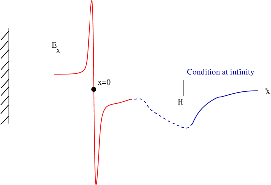
Figure 5: Schematic representation of the real part of the limit electric field of the second basis function $U_{2}^{\theta,\nu}$, $\nu>0$. Here the transversality condition $\sigma(\theta)\neq 0$ is satisfied, which turns into a singular behavior at the limit $\nu\rightarrow 0$.

5.4.3 Continuity estimates

The integral equation (3.9) is singular at the limit. The whole problem comes form the singularity at $x=0$. By comparison with the standard literature [33, 28, 35, 14, 29, 3, 32] we found no convenient mathematical tool to analyze its properties. That is why we develop in the following new continuity estimates with respect to the parameters of the problem. On this basis we will manage to pass to to the limit $\nu\rightarrow 0$.

Let us consider a general solution $\mathbf{U}=(U,V,W)\in\mathbb{X}^{\theta,\nu}$ of the integral equation (3.9) with prescribed data in $H$ under the form

$$V(H)=a_{H}\mbox{ and }W(H)=b_{H}.$$

Let us introduce the compact notation

$$\|H\|=\left|a_{H}\right|+\left|b_{H}\right|.$$

Our goal is to obtain some sharp continuity estimates on the solution $\mathbf{U}$ with respect to $\|H\|$. The main point is to bound the constants uniformly with respect to $0<\nu\leq 1$ which is hereafter taken positive for the simplicity of notation. The reference point can be different from $H$ as well, but non equal to zero. Once these continuity estimates are proved, they will provide enough information to define the limit $\nu\rightarrow 0$ of the second basis function.

Proposition 5.9.

There exists a constant $C_{\theta}$ with continuous dependence with respect to $\theta$ such that

$$\left|U(x)\right|\leq\frac{C_{\theta}}{\sqrt{r^{2}x^{2}+\nu^{2}}}\|H\|,\qquad 0<x\leq H.$$ (5.22)

Proof.

Let us consider

$$\gamma_{\theta}=\left(\sup_{0\leq\nu\leq 1}\|A_{\nu}\|_{W^{1,\infty}(0,H)}+\sup_{0\leq\nu\leq 1}\|B_{\nu}\|_{W^{1,\infty}(0,H)}\right)(\|\delta\|_{\infty}+|\theta|).$$

The integral equation (3.9) with $G=H$ implies that

$$\left|U(x)\right|\leq\frac{\gamma_{\theta}\|H\|}{\sqrt{r^{2}x^{2}+\nu^{2}}}+\int_{x}^{H}\frac{|\mathcal{D}_{x}^{\theta}\mathcal{D}_{z}^{\theta}k(x,z)|}{\sqrt{r^{2}x^{2}+\nu^{2}}}|U(z)|dz,$$

where we used (H2). Since $\mathcal{D}_{x}^{\theta}\mathcal{D}_{z}^{\theta}k(x,x)=0$ for all $x$, there exists a constant $\beta_{\theta}$ such that

$$\left\|\mathcal{D}_{x}^{\theta}\mathcal{D}_{z}^{\theta}k(x,z)\right\|_{L^{\infty}]0,H[}\leq\beta_{\theta}{|x-z|}\leq\beta_{\theta}z\quad\mbox{ for }0\leq x\leq z.$$

So $\sqrt{r^{2}x^{2}+\nu^{2}}|U(x)|\leq\gamma_{\theta}\|H\|+\beta_{\theta}\int_{x}^{H}z|U(z)|dz$ and

$$rx|U(x)|\leq\gamma_{\theta}\|H\|+\beta_{\theta}\int_{x}^{H}z|U(z)|dz,\qquad 0\leq x\leq H.$$

The Gronwall lemma is useful to study this inequality. Indeed let us set $g(x)=\int_{x}^{H}|zU(z)|dz$, so that the previous inequality is rewritten as $-rg^{\prime}(x)\leq\gamma_{\theta}\|H\|+\beta_{\theta}g(x)$. Therefore $0\leq\gamma_{\theta}\|H\|+rg^{\prime}(x)+\beta_{\theta}g(x)$, that is: $0\leq\gamma_{\theta}\|H\|e^{\frac{\beta_{\theta}}{r}x}+r\left(e^{\frac{\beta_{\theta}}{r}x}g(x)\right)^{\prime}$. Next we integrate on the interval $[x,H]$ and use the fact that $g(H)=0$ by definition. It yields $0\leq\gamma_{\theta}\|H\|\frac{e^{\frac{\beta_{\theta}}{r}H}-e^{\frac{\beta_{\theta}}{r}x}}{\frac{\beta_{\theta}}{r}}-re^{\frac{\beta_{\theta}}{r}x}g(x)$, that is

$$g(x)\leq\frac{e^{\frac{\beta_{\theta}}{r}(H-x)}-1}{\beta_{\theta}}\;\gamma_{\theta}\|H\|.$$ (5.23)

Finally one checks that $\sqrt{r^{2}x^{2}+\nu^{2}}|U(x)|\leq\gamma_{\theta}\|H\|+\beta_{\theta}g(x)\leq e^{\frac{\beta_{\theta}}{r}(H-x)}\gamma_{\theta}\|H\|$ which proves (5.22). ∎

Next define $\|0\|=\left|V(0)\right|+\left|W(0)\right|$.

Proposition 5.10.

There exists a constant $C_{\theta}$ with continuous dependence with respect to $\theta$ such that

$$\|0\|\leq C_{\theta}(1+|\ln\nu|)\|H\|.$$ (5.24)

Proof.

We adopt the same notations as above. The integral expression of $V$ (3.12) with $G=H$ yields the inequality

$$\left|V(0)\right|\leq\gamma_{\theta}\left\|H\right\|+\left|\int_{0}^{H}\mathcal{D}_{z}^{\theta}k(0,z)U(z)\right|dz$$

We notice that $\mathcal{D}_{z}^{\theta}k(0,z)=\left(\mathcal{D}_{z}^{\theta}k(0,z)-\mathcal{D}_{z}^{\theta}k(0,0)\right)+\mathcal{D}_{z}^{\theta}k(0,0)$. Since $\mathcal{D}_{z}^{\theta}k(0,0)=i\theta\partial_{z}k(0,0)-i\delta k(0,0)=i\theta$ one gets $\left|\mathcal{D}_{z}^{\theta}k(0,z)-i\theta\right|\leq\eta_{\theta}|z|$ for some constant $\eta_{\theta}>0$. Which gives

$$\left|V(0)\right|\leq\underbrace{\gamma_{\theta}\left\|H\right\|+\eta_{\theta}\int_{0}^{H}z|U(z)|dz}_{Q}+|\theta|\underbrace{\left|\int_{0}^{H}U(z)dz\right|}_{R}.$$

By (5.22) $Q\leq C_{\theta}\|H\|$, and moreover,

$$R:=\left|\int_{0}^{H}U(z)dz\right|\leq C_{\theta}\|H\|\left|\int_{0}^{H}\frac{1}{r|x|+\nu}dz\right|\leq C_{\theta}\|H\||\ln\nu|.$$

This completes the proof for $|V_{2}(0)|$. The term $|W(0)|$ is bounded with the same method starting from the integral (3.13) and using the identity $\partial_{x}\mathcal{D}_{z}^{\theta}k_{\nu}(x,x)=i\delta(z)A_{\nu}(z)$. ∎

An interesting question is the following. Let us consider the integral equation (3.9) with $G=0$. That is the starting point of the integral is the singularity. One may wonder if a direct use of the Gronwall lemma may yield valuable estimates, or not. It appears that a pollution with $\log\nu$ terms render the result of little interest.

Consider firstly for simplicity $0\leq x$. Then (3.9) with $G=0$ turns into

$$\left|U(x)\right|\leq C_{\theta}\frac{\|0\|}{\sqrt{r^{2}x^{2}+\nu^{2}}}+C\int_{0}^{x}\left|U(z)\right|dz$$ (5.25)

where we used (4.4) to bound the kernel. The constant $C_{\theta}>0$ is chosen large enough. Set $h(x)=\int_{0}^{x}\left|U(z)\right|dz$ so that $h^{\prime}(x)\leq C_{\theta}\frac{\|0\|}{\sqrt{r^{2}x^{2}+\nu^{2}}}+C_{\theta}h(x)$. Since $h(0)=0$ the Gronwall lemma yields the inequality $h(x)\leq C_{\theta}^{\prime}\int_{0}^{x}\frac{\|0\|}{|z|+|\nu|}dz$ that is after integration ($0\leq x\leq H$) $\left|h(x)\right|\leq C_{\theta}^{\prime\prime}\|0\|\left(1+|\ln\nu|\right),$ for some constant $C_{\theta}^{\prime\prime}>0$ with continuous dependence with respect to $\theta$. Considering the bound (5.24) and the symmetry between $0<x$ and $x<0$ in the integral (3.9) (with $G=0$) one obtains the estimate

$$\left|\int_{0}^{x}U(z)dz\right|\leq C_{\theta}^{\prime\prime\prime}\|H\|\left(1+|\ln\nu|\right)^{2},\quad-L\leq x\leq H.$$ (5.26)

Going back to (5.25) which is easily generalized to $x<0$, one gets

$$\left|U(x)\right|\leq C_{\theta}\left(\frac{1}{\sqrt{r^{2}x^{2}+\nu^{2}}}+1+|\ln\nu|\right)\left(1+|\ln\nu|\right)\|H\|,\quad-L\leq x\leq H.$$ (5.27)

By comparison of (5.22) and (5.27), it is clear that this technique generates spurious terms of order $\log\nu$ for positive $x$. It spoils the possibility of having sharp estimates also for negative $x$. With this respect, the rest of this section is devoted to the derivation of various sharp inequalities which are free of such spurious terms.

Let us define

$$Q(\mathbf{U})=V_{1}^{\theta,\nu}(H)W(H)-W_{1}^{\theta,\nu}(H)V(H).$$ (5.28)

This quantity is the Wronskian of the current solution $\mathbf{U}$ against the first basis function. It is therefore independent of the position $H$ which is used to evaluate $Q(\mathbf{U})$.

Proposition 5.11.

There exists a constant $C_{\theta}$ with continuous dependence with respect to $\theta$ and a continuous function $\nu\mapsto\varepsilon(\nu)$ with $\varepsilon(0)=0$ such that

$$\left|\;|\nu|\left\|U\right\|^{2}_{L^{2}(-L,H)}-\left|\frac{\pi Q(\mathbf{U})^{2}}{\alpha^{\prime}(0)}\right|\;\right|\leq C_{\theta}\varepsilon(\nu)\|H\|^{2}.$$ (5.29)

Proof.

We consider positive $\nu$ to simplify the notations. The proof is easily adapted for negative $\nu$.

Consider the integral equation (3.9) with $G=0$. One gets

$$U(x)=\frac{a_{0}\mathcal{D}_{x}^{\theta}A(x)+b_{0}\mathcal{D}_{x}^{\theta}B(x)}{\alpha(x)+i\nu}+\int_{0}^{x}\frac{\mathcal{D}_{x}^{\theta}\mathcal{D}_{z}^{\theta}k(x,z)}{\alpha(x)+i\nu}U(z)dz.$$

Here $(a_{0},b_{0})$ are a priori different from $(a_{H},b_{H})$. Due to (5.28), the normalization of $\mathbf{U}_{1}$ and thanks to Lemma 5.1 one has that $a_{0}\mathcal{D}_{x}^{\theta}A(0)+b_{0}\mathcal{D}_{x}^{\theta}B(0)=Q(\mathbf{U})$. So the integral equation can be written as

$$U(x)=\underbrace{\frac{Q(\mathbf{U})}{\alpha(x)+i\nu}}_{S_{1}}$$ (5.30)

$$+\underbrace{a_{0}\frac{\mathcal{D}_{x}^{\theta}A(x)-\mathcal{D}_{x}^{\theta}A(0)}{\alpha(x)+i\nu}+b_{0}\frac{\mathcal{D}_{x}^{\theta}B(x)-\mathcal{D}_{x}^{\theta}B(0)}{\alpha(x)+i\nu}}_{S_{2}}+\underbrace{\int_{0}^{x}\frac{\mathcal{D}_{x}^{\theta}\mathcal{D}_{z}^{\theta}k(x,z)}{\alpha(x)+i\nu}U(z)dz}_{S_{3}}.$$

• The $L^{2}$ norm of the first term $S_{1}$ depends upon the value of

  $$D_{\nu}=\int_{-L}^{H}\frac{\nu}{\alpha(x)^{2}+\nu^{2}}dx.$$

  Make the change of variable $x=\nu w$ so that $D_{\nu}=\int_{-\frac{L}{\nu}}^{\frac{H}{\nu}}\frac{1}{b_{\nu}(w)^{2}+1}dw$ and $b_{\nu}(w)=\frac{\alpha(\nu w)}{\nu}$. Using the hypothesis (H2) one has that $|b_{\nu}(w)|\geq rw$, $r>0$. Since $\int_{\mathbb{R}}\frac{dw}{r^{2}w^{2}+1}=\frac{\pi}{r}<\infty$ and the point-wise limit of $b_{\nu}(x)$ is $\alpha^{\prime}(0)x$, the Lebesgue dominated convergence theorem states that $\lim_{0^{+}}D_{\nu}=\frac{\pi}{|\alpha^{\prime}(0)|}$. Considering that

  $$\left|Q(\mathbf{U})\right|\leq C_{\theta}^{1}\|H\|$$ (5.31)

  using (5.28), there exists a continuous function $\nu\mapsto\varepsilon^{1}(\nu)$ with $\varepsilon^{1}(0)=0$ such that

  $$\left|\nu\|S_{1}\|_{L^{2}(-L-,H)}^{2}-\left|\frac{\pi Q(\mathbf{U})^{2}}{\alpha^{\prime}(0)}\right|\right|\leq C_{\theta}^{1}\varepsilon^{1}(\nu)\|H\|^{2}.$$ (5.32)

• The functions $\frac{\mathcal{D}_{x}^{\theta}A_{\nu}(x)-\mathcal{D}_{x}^{\theta}A_{\nu}(0)}{\alpha(x)+i\nu}$ and $\frac{\mathcal{D}_{x}^{\theta}B_{\nu}(x)-\mathcal{D}_{x}^{\theta}B_{\nu}(0)}{\alpha(x)+i\nu}$ can bounded in $L^{\infty}$ uniformly with respect to $\nu$. So $\int_{-L}^{H}|S_{2}(z)|^{2}dz\leq c^{2}_{\theta}\|0\|^{2}$. Estimate (5.24) yields

  $$\nu\|S_{2}\|_{L^{2}(-L-,H)}^{2}\leq C_{\theta}^{2}\nu(1+|\ln\nu|)^{2}\|H\|^{2},\qquad C_{\theta}^{2}>0.$$ (5.33)

• The last term $S_{3}$ is

  $$|S_{3}(x)|=\left|\int_{0}^{x}\frac{\mathcal{D}_{x}^{\theta}\mathcal{D}_{z}^{\theta}k^{\nu}(x,z)}{\alpha(x)+i\nu}U(z)dz\right|\leq c_{3}^{\theta}\left|\int_{0}^{x}|U(z)|dz\right|$$

  since the kernel is bounded (4.4) with respect to $\theta$ and uniformly for $\nu\in[0,1]$. Inequality (5.26) implies that $|S_{3}(x)|\leq c_{\theta}^{3}\left(1+|\ln\nu|\right)^{2}\|H\|$. Therefore this term is bounded like

  $$\nu\|S_{3}\|_{L^{2}(-L-,H)}^{2}\leq c_{\theta}^{4}\nu\left(1+|\ln\nu|\right)^{4}\|H\|^{2},\qquad c_{\theta}^{4}>0.$$ (5.34)

We complete the proof adding the three inequalities (5.32-5.34). ∎

To pursue the analysis, we begin by rewriting the general form of the integral equation (3.9), showing that the various singularities of the equation can be recombined under a more convenient form. This intermediate result is essential to obtain all following results. Indeed the integral equation for $U$ (3.9) choosing $G=0$ writes

$$(\alpha(x)+i\nu)U(x)=a_{0}\mathcal{D}_{x}^{\theta}A_{\nu}(x)+b_{0}\mathcal{D}_{x}^{\theta}B_{\nu}(x)+\int_{0}^{x}\mathcal{D}_{x}^{\theta}\mathcal{D}_{z}^{\theta}k^{\nu}(x,z)U(z)dz.$$

Since by construction $a_{0}\mathcal{D}_{x}^{\theta}A_{\nu}(0)+b_{0}\mathcal{D}_{x}^{\theta}B_{\nu}(0)=Q(\mathbf{U})$ one also has

$$(\alpha(x)+i\nu)U(x)=a_{0}\left(\mathcal{D}_{x}^{\theta}A_{\nu}(x)-\mathcal{D}_{x}^{\theta}A_{\nu}(0)\right)+b_{0}\left(\mathcal{D}_{x}^{\theta}B_{\nu}(x)-\mathcal{D}_{x}^{\theta}B_{\nu}(0)\right)$$

$$+Q(\mathbf{U})+\int_{0}^{x}\mathcal{D}_{x}^{\theta}\mathcal{D}_{z}^{\theta}k^{\nu}(x,z)U(z)dz.$$

But one also has due to the integral equation for $V$ (3.12) choosing $G=H$

$$V(0)=a_{0}=a_{H}A_{\nu}(0)+b_{H}B_{\nu}(0)-\int_{0}^{H}\mathcal{D}_{z}^{\theta}k^{\nu}(0,z)U(z)dz.$$

Basic manipulations yield

$$a_{0}=a_{H}-\int_{0}^{H}\left(\mathcal{D}_{z}^{\theta}k^{\nu}(0,z)-\mathcal{D}_{z}^{\theta}k^{\nu}(0,0)\right)U(z)dz-i\theta\int_{0}^{H}U(z)dz$$

because $\mathcal{D}_{z}^{\theta}k^{\nu}(0,0)=i\theta$. Since the function $\mathcal{D}_{z}^{\theta}k^{\nu}$ is continuous, there exists a constant $C_{4}^{\theta}$ independent of $\nu$ such that

$$\left|\mathcal{D}_{z}^{\theta}k^{\nu}(x,z)-\mathcal{D}_{z}^{\theta}k^{\nu}(x,x)\right|\leq C_{4}^{\theta}(z-x)\leq C_{4}^{\theta}z\quad\mbox{ for }0\leq x\leq z\leq H.$$

Therefore the integral $\int_{0}^{H}\left|\mathcal{D}_{z}^{\theta}k^{\nu}(0,z)-\mathcal{D}_{z}^{\theta}k^{\nu}(0,0)\right||U(z)|dz\leq C_{4}^{\theta}\int_{0}^{H}z|U(z)|dz$ is bounded uniformly with respect to $\nu$ thanks to the bound given in (5.22). We summarize this as

$$a_{0}=\tilde{a}-i\theta\int_{0}^{H}U(z)dz$$ (5.35)

where $|\tilde{a}|\leq C_{5}^{\theta}\|H\|$ is bounded uniformly with respect to $\nu$. Similarly

$$b_{0}=b_{H}-\int_{0}^{H}\partial_{x}\mathcal{D}_{z}^{\theta}k^{\nu}(0,z)U(z)dz$$ (5.36)

and since the function $\partial_{x}\mathcal{D}_{z}^{\theta}k^{\nu}$ is continuous and $\partial_{x}\mathcal{D}^{\theta}_{z}(0,0)=i\delta(0)$

$$b_{0}=\tilde{b}-i\int_{0}^{H}\delta(0)U(z)dz$$ (5.37)

where $\tilde{b}$ is also bounded uniformly with respect to $\nu$: $|\tilde{b}|\leq C_{6}^{\theta}\|H\|$. The integral equation then gives

$$(\alpha(x)+i\nu)U(x)=\tilde{a}\left(\mathcal{D}_{x}^{\theta}A_{\nu}(x)-\mathcal{D}_{x}^{\theta}A_{\nu}(0)\right)+\tilde{b}\left(\mathcal{D}_{x}^{\theta}B_{\nu}(x)-\mathcal{D}_{x}^{\theta}B_{\nu}(0)\right)$$

$$+Q(\mathbf{U})-\int_{0}^{H}Q(x,z)U(z)dz+\int_{0}^{x}\mathcal{D}_{x}^{\theta}\mathcal{D}_{z}^{\theta}k^{\nu}(x,z)U(z)dz$$

where the new kernel is

$$Q(x,z)=\left(\mathcal{D}_{x}^{\theta}A_{\nu}(x)-\mathcal{D}_{x}^{\theta}A_{\nu}(0)\right)i\theta+\left(\mathcal{D}_{x}^{\theta}B_{\nu}(x)-\mathcal{D}_{x}^{\theta}B_{\nu}(0)\right)i\delta(0)$$

$$=\mathcal{D}_{x}^{\theta}A^{\nu}(x)\mathcal{D}_{z}^{\theta}B_{\nu}(0)-\mathcal{D}_{x}^{\theta}B^{\nu}(x)\mathcal{D}_{z}^{\theta}A_{\nu}(0)=\mathcal{D}_{x}^{\theta}\mathcal{D}_{z}^{\theta}k^{\nu}(x,0)$$

after evident simplifications. It is convenient to introduce two bounded functions $m^{\theta,\nu}=\frac{\mathcal{D}_{x}^{\theta}A^{\nu}(x)-\mathcal{D}_{x}^{\theta}A_{\nu}(0)}{x}$ and $n^{\theta,\nu}=\frac{\mathcal{D}_{x}^{\theta}B^{\nu}(x)-\mathcal{D}_{x}^{\theta}B_{\nu}(0)}{x}$ so that (3.9) is rewritten as

$$(\alpha(x)+i\nu)U(x)=\tilde{a}m^{\theta,\nu}(x)x+\tilde{b}n^{\theta,\nu}(x)x+Q(\mathbf{U})-\int_{x}^{H}\mathcal{D}_{x}^{\theta}\mathcal{D}_{z}^{\theta}k^{\nu}(x,0)U(z)dz$$ (5.38)

$$+\int_{0}^{x}\left(\mathcal{D}_{x}^{\theta}\mathcal{D}_{z}^{\theta}k^{\nu}(x,z)-\mathcal{D}_{x}^{\theta}\mathcal{D}_{z}^{\theta}k^{\nu}(x,0)\right)U(z)dz,\quad\forall x\in[-L,\infty[.$$

A first property which shows that (5.38) is less singular that its initial form (3.9) is the following lemma which uses the pointwise estimate (5.22) on $U$ (so an important restriction is nevertheless that $x>0$).

Lemma 5.3.

The first component $U$ of any element $\mathbf{U}\in\mathbb{X}^{\theta,\nu}$ satisfies

$$(\alpha(x)+i\nu)U(x)=p^{\theta,\nu}(x)x+Q(\mathbf{U})-\int_{x}^{H}\mathcal{D}_{x}^{\theta}\mathcal{D}_{z}^{\theta}k^{\nu}(x,0)U(z)dz$$ (5.39)

where

$$\|p^{\theta,\nu}\|_{L^{\infty}(0,H)}\leq C^{\theta}\|H\|,\qquad\forall\nu\in[0,1].$$ (5.40)

Proof.

Let us focus on the second integral in (5.38). Continuity properties with respect to the second variable $z$ imply that there exists a constant $C_{7}^{\theta}$ independent of $\nu$ such that

$$\left|\mathcal{D}_{x}^{\theta}\mathcal{D}_{z}^{\theta}k^{\nu}(x,z)-\mathcal{D}_{x}^{\theta}\mathcal{D}_{z}^{\theta}k^{\nu}(x,0)\right|\leq C_{7}^{\theta}z.$$ (5.41)

So, for $x\geq 0$,

$$\left|\int_{0}^{x}\left(\mathcal{D}_{x}^{\theta}\mathcal{D}_{z}^{\theta}k^{\nu}(x,z)-\mathcal{D}_{x}^{\theta}\mathcal{D}_{z}^{\theta}k^{\nu}(x,0)\right)U(z)dz\right|\leq C_{7}^{\theta}\int_{0}^{x}z|U(z)|dz\leq C_{7}^{\theta}C_{\theta}\|H\|x$$

using estimate (5.22). Set

$$p^{\theta,\nu}(x)=\tilde{a}m^{\theta,\nu}(x)+\tilde{b}n^{\theta,\nu}(x)+\frac{1}{x}\int_{0}^{x}\left(\mathcal{D}_{x}^{\theta}\mathcal{D}_{z}^{\theta}k^{\nu}(x,z)-\mathcal{D}_{x}^{\theta}\mathcal{D}_{z}^{\theta}k^{\nu}(x,0)\right)U(z)dz$$ (5.42)

which satisfies by construction (5.40). ∎

As a consequence one has

Proposition 5.12.

For all $1\leq p<\infty$, there exists a constant $C_{p}^{\theta}$ independent of $\nu$ and which depends continuously on $\theta$ such that

$$\left\|U-\frac{Q(\mathbf{U})}{\alpha(\cdot)+i\nu}\right\|_{L^{p}(0,H)}\leq C_{p}^{\theta}\|H\|.$$ (5.43)

Proof.

From lemma 5.3 one has that

$$U(x)-\frac{Q(\mathbf{U})}{\alpha(x)+i\nu}=\frac{x}{\alpha(x)+i\nu}p^{\theta,\nu}(x)-\frac{\mathcal{D}_{x}^{\theta}\mathcal{D}_{z}^{\theta}k^{\nu}(x,0)}{\alpha(x)+i\nu}\int_{x}^{H}U(z)dz,$$

which turns into

$$\left(U(x)-\frac{Q(\mathbf{U})}{\alpha(x)+i\nu}\right)+\frac{\mathcal{D}_{x}^{\theta}\mathcal{D}_{z}^{\theta}k^{\nu}(x,0)}{\alpha(x)+i\nu}\int_{x}^{H}\left(U(z)-\frac{Q(\mathbf{U})}{\alpha(z)+i\nu}\right)dz$$

$$=\frac{x}{\alpha(x)+i\nu}p^{\theta,\nu}(x)-Q(\mathbf{U})\frac{\mathcal{D}_{x}^{\theta}\mathcal{D}_{z}^{\theta}k^{\nu}(x,0)}{\alpha(x)+i\nu}\int_{x}^{H}\frac{1}{\alpha(z)+i\nu}dz$$ (5.44)

By virtue of (H2) we notice that $\left|\int_{x}^{H}\frac{1}{\alpha(z)+i\nu}dz\right|\leq\int_{x}^{H}\frac{1}{|\alpha(z)|}dz\leq\frac{1}{r}\log(H/x)$. Since all powers of the function $x\mapsto\ln|x|$ are integrable, the right-hand side (5.44) is naturally bounded in any $L^{p}$, $1\leq p<\infty$. Therefore the function $Z(x)=U(x)-\frac{Q(\mathbf{U})}{\alpha(x)+i\nu}$ is solution of an integral equation with a bounded kernel and a right hand side in $L^{p}$. The form of this integral equation is

$$Z(x)+\widetilde{K}^{\theta,\nu}(x)\int_{x}^{H}Z(z)dz=b^{\theta,\nu}(x)$$

with $\left\|\widetilde{K}^{\theta,\nu}(x)\right\|_{L^{\infty}(0,H)}\leq C_{8}^{\theta}$ independently of $\nu$. One also uses $\left\|b^{\theta,\nu}\right\|_{L^{p}(0,H)}\leq c_{p}^{\theta}\|H\|$ for $0\leq\nu\leq 1$: the key estimate is (5.40) which explains why the result is restricted to $x>0$ . Since this is a standard non-singular integral equation, see [33], the claim is proved. ∎

The previous result (5.43) shows that some singularities of the integral equation can be recombined in a less singular formulation, so that the dominant part of $U$ is $\frac{1}{\alpha(\cdot)+i\nu}$. An important restriction of this technique, for the moment, is that it needs the a priori estimate (5.22) on $U$. This explains why inequality (5.43) is restricted to $x>0$. By inspection of the structure of the algebra, it appears that one has the same kind of inequalities on the entire interval by replacing $U$ directly by the function $\frac{1}{\alpha(\cdot)+i\nu}$ in the integrals. A preliminary and fundamental result in this direction concerns the function

$$D^{\theta,\nu}(x)=-\frac{\mathcal{D}_{x}^{\theta}\mathcal{D}_{z}^{\theta}k^{\nu}(x,0)}{\alpha(x)+i\nu}\int_{0}^{H}\frac{1}{\alpha(z)+i\nu}dz+\int_{0}^{x}\frac{\mathcal{D}_{x}^{\theta}\mathcal{D}_{z}^{\theta}k^{\nu}(x,z)}{\alpha(x)+i\nu}\frac{1}{\alpha(z)+i\nu}dz$$

which is nothing than the integral part of (5.38) where $U$ is replaced by the function $\frac{1}{\alpha(\cdot)+i\nu}$.

Proposition 5.13.

Let $1\leq p<\infty$. One has $\left\|D^{\theta,\nu}\right\|_{L^{p}(-L,H)}\leq C_{p}^{\theta}$ where the constant depends continuously on $\theta$ and does not depend on $\nu$.

Proof.

Two cases occur.

• Assume $0\leq x\leq H$. The analysis is similar to the one of proposition 5.12. One has the same kind of rearrangement (5.38), that is

  $$D^{\theta,\nu}(x)=-\frac{\mathcal{D}_{x}^{\theta}\mathcal{D}_{z}^{\theta}k^{\nu}(x,0)}{\alpha(x)+i\nu}\int_{x}^{H}\frac{1}{\alpha(z)+i\nu}dz$$

  $$+\int_{0}^{x}\frac{\mathcal{D}_{x}^{\theta}\mathcal{D}_{z}^{\theta}k^{\nu}(x,z)-\mathcal{D}_{x}^{\theta}\mathcal{D}_{z}^{\theta}k^{\nu}(x,0)}{\alpha(x)+i\nu}\frac{1}{\alpha(z)+i\nu}dz.$$

  The first term is bounded like $C^{\theta}\frac{|\log x|}{r}$ which is in all $L^{p}$, $p<\infty$. The second term is immediately bounded using (5.41): indeed

  $$\left|\int_{0}^{x}\frac{\mathcal{D}_{x}^{\theta}\mathcal{D}_{z}^{\theta}k^{\nu}(x,z)-\mathcal{D}_{x}^{\theta}\mathcal{D}_{z}^{\theta}k^{\nu}(x,0)}{\alpha(x)+i\nu}\frac{1}{\alpha(z)+i\nu}dz\right|$$

  $$\leq C_{7}^{\theta}\frac{1}{\sqrt{\alpha(x)^{2}+\nu^{2}}}\int_{0}^{x}\frac{z}{\sqrt{\alpha(z)^{2}+\nu^{2}}}dz\leq C_{7}^{\theta}\frac{1}{r^{2}}.$$

• Assume $-L\leq x\leq 0$. The decomposition is slightly different and uses some cancellations permitted by the symmetry properties of the kernels. One has

  $$D^{\theta,\nu}(x)=-\frac{\mathcal{D}_{x}^{\theta}\mathcal{D}_{z}^{\theta}k^{\nu}(x,0)}{\alpha(x)+i\nu}\int_{-x}^{H}\frac{1}{\alpha(z)+i\nu}dz$$

  $$+\int_{0}^{x}\frac{\mathcal{D}_{x}^{\theta}\mathcal{D}_{z}^{\theta}k^{\nu}(x,z)}{\alpha(x)+i\nu}\frac{1}{\alpha(z)+i\nu}dz-\frac{\mathcal{D}_{x}^{\theta}\mathcal{D}_{z}^{\theta}k^{\nu}(x,0)}{\alpha(x)+i\nu}\int_{0}^{-x}\frac{1}{\alpha(z)+i\nu}dz,$$

  which emphasizes the importance of some symmetry properties of the kernels. Indeed

  $$\int_{0}^{-x}\frac{1}{\alpha(z)+i\nu}dz=-\int_{0}^{x}\frac{1}{\alpha(-w)+i\nu}dw$$

  $$=\int_{0}^{x}\frac{1}{\alpha(w)+i\nu}dw+\int_{0}^{x}\left(\frac{1}{-\alpha(-w)-i\nu}-\frac{1}{\alpha(w)+i\nu}\right)dw.$$

  Notice that

  $$\frac{1}{-\alpha(-w)-i\nu}-\frac{1}{\alpha(w)+i\nu}=\frac{\alpha(w)+\alpha(-w)+2i\nu}{(\alpha(w)+i\nu)(-\alpha(-w)-i\nu)}.$$

  So, since $\alpha(0)=0$,

  $$\left|\frac{1}{-\alpha(-w)-i\nu}-\frac{1}{\alpha(w)+i\nu}\right|\leq\frac{2\left\|\alpha\right\|_{W^{2,\infty}(-L,H)}w^{2}+2\nu}{r^{2}w^{2}+\nu^{2}},$$

  since $\alpha\in W^{2,\infty}(-L,H)$. One can bound

  $$\left|\int_{0}^{x}\frac{1}{-\alpha(-w)-i\nu}dw-\int_{0}^{x}\frac{1}{\alpha(w)+i\nu}dw\right|\leq\frac{\left\|\alpha\right\|_{W^{2,\infty}(-L,H)}}{r^{2}}|x|+\int_{0}^{x}\frac{2\nu}{r^{2}z^{2}+\nu^{2}}dz$$

  $$\leq\frac{\left\|\alpha\right\|_{W^{2,\infty}(-L,H)}}{r^{2}}\max(H,L)+\int_{0}^{\infty}\frac{2\nu}{r^{2}z^{2}+\nu^{2}}dz\leq\frac{\left\|\alpha\right\|_{W^{2,\infty}(-L,H)}}{r^{2}}\max(H,L)+\frac{\pi}{r}.$$

  As a consequence $D^{\theta,\nu}$ can be expressed as

  $$D^{\theta,\nu}(x)=-\frac{\mathcal{D}_{x}^{\theta}\mathcal{D}_{z}^{\theta}k^{\nu}(x,0)}{\alpha(x)+i\nu}\int_{-x}^{H}\frac{1}{\alpha(z)+i\nu}dz$$

  $$+\int_{0}^{x}\frac{\mathcal{D}_{x}^{\theta}\mathcal{D}_{z}^{\theta}k^{\nu}(x,z)-\mathcal{D}_{x}^{\theta}\mathcal{D}_{z}^{\theta}k^{\nu}(x,0)}{\alpha(x)+i\nu}\frac{1}{\alpha(z)+i\nu}dz+R(x)$$

  with $\left\|R\right\|_{\infty}(-L,H)\leq C_{10}^{\theta}$. The two integrals have the same structure as for the first case, in particular the interval of integration is $[-x,H]$ with $0\leq-x$. So the same result holds.

∎

Proposition 5.14.

For all $1\leq p<\infty$, there exists a constant $C_{p}^{\theta}$ independent of $\nu$ such that

$$\left\|U-\frac{Q(\mathbf{U})}{\alpha(\cdot)+i\nu}\right\|_{L^{p}(-L,H)}\leq C_{p}^{\theta}\|H\|.$$ (5.45)

Proof.

We start from (5.38) written as

$$U(x)=\frac{Q(\mathbf{U})}{\alpha(x)+i\nu}+\frac{x}{\alpha(x)+i\nu}\widetilde{p}^{\theta,\nu}(x)$$

$$-\int_{0}^{H}\frac{\mathcal{D}_{x}^{\theta}\mathcal{D}_{z}^{\theta}k^{\nu}(x,0)}{\alpha(x)+i\nu}U(z)dz+\int_{0}^{x}\frac{\mathcal{D}_{x}^{\theta}\mathcal{D}_{z}^{\theta}k^{\nu}(x,z)}{\alpha(x)+i\nu}U(z)dz.$$

Here $\widetilde{p}^{\theta,\nu}(x)=\tilde{a}m^{\theta,\nu}(x)+\tilde{b}n^{\theta,\nu}(x)$, so that $\|\widetilde{p}^{\theta,\nu}\|_{L^{\infty}(-L,H)}\leq C^{\theta}\|H\|$ over the whole interval $(-L,H)$. Notice that $\widetilde{p}^{\theta,\nu}$ is the first part of ${p}^{\theta,\nu}$ defined in (5.42). Setting $u(x)=U(x)-\frac{Q(\mathbf{U})}{\alpha(x)+i\nu}$ one gets

$$u(x)-\int_{0}^{x}\frac{\mathcal{D}_{x}^{\theta}\mathcal{D}_{z}^{\theta}k^{\nu}(x,z)}{\alpha(x)+i\nu}u(z)dz$$

$$=\frac{x}{\alpha(x)+i\nu}\widetilde{p}^{\theta,\nu}(x)-Q(\mathbf{U})D^{\theta,\nu}(x)-\int_{0}^{H}\frac{\mathcal{D}_{x}^{\theta}\mathcal{D}_{z}^{\theta}k^{\nu}(x,0)}{\alpha(x)+i\nu}u(z)dz.$$

The left-hand side is an non singular integral operator of the second kind with a bounded kernel thanks to the fundamental property (4.4). The right-hand side is bounded in $L^{p}$ with a continuous dependence with respect to $\|H\|$, see Lemma 5.3, estimation (5.31) and estimation (5.43).

∎

5.4.4 The second basis function

We apply the above material to the second basis function for which $Q(\mathbf{U}_{2}^{\theta,\nu})=1$. The inequality (5.45) writes

$$\left\|U_{2}^{\theta,\nu}-\frac{1}{\alpha(\cdot)+i\nu}\right\|_{L^{p}(-L,H)}\leq C_{p}^{\theta}\left(\left|V_{2}^{\theta,\nu}(H)\right|+\left|W_{2}^{\theta,\nu}(H)\right|\right),$$ (5.46)

for $1\leq p<\infty$.

Proposition 5.15.

Assume the transversality condition (5.21). There exists a constant $C^{\theta}$ independent of $\nu$ and continuous with respect to $\theta$ such that

$$\left|V_{2}^{\theta,\nu}(H)\right|+\left|W_{2}^{\theta,\nu}(H)\right|\leq C^{\theta}.$$ (5.47)

Proof.

Indeed, regarding relation (5.16), (5.17) the pair $(v,w)=(V_{2}^{\theta,\nu}(H),W_{2}^{\theta,\nu}(H))$ is solution of the linear system

$$\left\{\begin{array}[]{ll}-vW_{1}^{\theta,\nu}(H)+wV_{1}^{\theta,\nu}(H)=1,\\ vW_{3}^{\theta,\nu}(H)-wV_{3}^{\theta,\nu}(H)=0.\end{array}\right.$$ (5.48)

The determinant of this linear system is equal to the value of the function $-\sigma(\theta,\nu)$. So the transversality condition establishes that

$$\mbox{det }\left(\begin{array}[]{ll}-W_{1}^{\theta,\nu}(H)&V_{1}^{\theta,\nu}(H)\\ W_{3}^{\theta,\nu}(H)&-V_{3}^{\theta,\nu}(H)\end{array}\right)=-\sigma(\theta,\nu)\neq 0.$$

Therefore the solution of the linear system

$$v=-\frac{V_{3}^{\theta,\nu}(H)}{\sigma(\theta,\nu)},\quad w=-\frac{W_{3}^{\theta,\nu}(H)}{\sigma(\theta,\nu)}$$ (5.49)

is bounded uniformly with respect to $\nu$. ∎

Theorem 5.2.

Assume the same transversality condition (5.21). The second basis function satisfies the following estimates for some $C_{p}^{\theta}$ and $C^{\theta}$ which are continuous with respect to $\theta$

$$\left\|U_{2}^{\theta,\nu}-\frac{1}{\alpha(\cdot)+i\nu}\right\|_{L^{p}(-L,H)}\leq C_{p}^{\theta},\quad 1\leq p<\infty,$$ (5.50)

$$\left\|\mathbf{U}^{\theta,\nu}_{2}\right\|_{H^{1}_{\rm loc}([-L,0)\cup(0,H])}\leq C^{\theta}.$$ (5.51)

Proof.

The first estimate is a straightforward consequence of (5.46), (5.47) . The use of the integral representations (3.12-3.13) shows that,

$$\left\|V_{2}^{\theta,\nu}\right\|_{L^{\infty}_{\rm loc}([-L,0)\cup(0,H])}+\left\|W_{2}^{\theta,\nu}\right\|_{L^{\infty}_{\rm loc}([-L,0)\cup(0,H])}\leq C^{\theta}$$ (5.52)

for some $C^{\theta}$. Then the second equation of (2.4) shows that one has the same bound for $U_{2}^{\theta,\nu}$

$$\left\|U_{2}^{\theta,\nu}\right\|_{L^{\infty}_{\rm loc}([-L,0)\cup(0,H])}\leq C^{\theta}.$$ (5.53)

The bound on the derivatives follows from (2.4) ∎

Remark 8.

Let us set $H^{\prime}=-L$. From (5.52) one gets that $\|H^{\prime}\|$ is bounded uniformly also, therefore (5.22) can be generalized for $x<0$ (resp. $H^{\prime}$) instead of $x>0$ (resp. $H$). In summary one has for a constant $K^{\theta}$ that can be further specified: $\left|U_{2}^{\theta,\nu}(x)\right|\leq\frac{K^{\theta}}{\sqrt{r^{2}x^{2}+\nu^{2}}}$ for $x\in(-L,H)$.

We now pass to the limit $\nu\rightarrow 0^{\pm}$.

Proposition 5.16.

Assume the same transversality condition (5.21). The second basis function admits a limit in the sense of distribution for $\nu=0^{\pm}$ as follows:

$$\mathbf{U}_{2}^{\theta,\nu}\rightarrow\mathbf{U}_{2}^{\theta,\pm}=\left(P.V.\frac{1}{\alpha(x)}\pm\frac{i\pi}{\alpha^{\prime}(0)}\delta_{D}+u_{2}^{\theta,\pm},\;v_{2}^{\theta,\pm},\;w_{2}^{\theta,\pm}\right)$$

where $u_{2}^{\theta,\pm},v_{2}^{\theta,\pm},w_{2}^{\theta,\pm}\in L^{2}(-L,\infty)$ and $\delta_{D}$ is the Dirac mass at the origin.

Remark 9.

The limits $\mathbf{U}_{2}^{\theta,\pm}$ are solutions of (2.4) in the sense of distribution. they will be called the singular solutions.

Proof.

We consider firstly the case $\nu\downarrow 0$. Some parts of the proof are already evident, essentially for quantities which are regular enough ($V_{2}^{\theta,\nu}$ and $W_{2}^{\theta,\nu}$) or for regions where all functions are regular (typically $x>0$). Therefore the whole point is to pass to the limit in the singular part of the solution $U_{2}^{\theta,\nu}$. We will make wide use of the equivalence between the integral formulation of proposition 3.1 and the differential formulation (2.4).

$\bullet$ Passing to the weak limit: By continuity of the first basis function with respect to $\nu$, one can pass to the limit concerning $(V_{2}^{\theta,\nu}(H),W_{2}^{\theta,\nu}(H))$. One gets that $(v,w)=(V_{2}^{\theta,0^{+}}(H),W_{2}^{\theta,0^{+}}(H))$ is the unique solution of the linear system

$$\left\{\begin{array}[]{ll}-vW_{1}^{\theta}(H)+wV_{1}^{\theta}(H)=1,\\ vW_{3}^{\theta}(H)-wV_{3}^{\theta}(H)=0,\end{array}\right.$$ (5.54)

where the coefficients are defined in terms of the first basis function for $\nu=0$. By continuity away from the singularity at $x=0$, one has that $\mathbf{U}_{2}^{\theta,\nu}\rightarrow\mathbf{U}_{2}^{\theta}$ in $L^{\infty}(\epsilon,H)$ for all $\epsilon>0$. Using (5.50) it is clear that $U^{\theta,\nu}-\frac{1}{\alpha(\cdot)+i\nu}$ is bounded in $L^{2}(-L,H)$ uniformly with respect to $\nu$. Therefore there exists a limit function denoted as $u_{2}^{\theta,0^{+}}$ such that for a subsequence: $U_{2}^{\theta,\nu}-\frac{1}{\alpha(\cdot)+i\nu}\rightarrow_{\rm weak}u_{2}^{\theta,0^{+}}$ in $L^{2}(-L,H)$. Moreover the first derivative of $U_{2}^{\theta,\nu}$ is bounded in $L^{2}(-L,-\epsilon)$ by virtue of (5.51). Therefore $U_{2}^{\theta,\nu}\rightarrow_{\rm strong}\frac{1}{\alpha(\cdot)}+u_{2}^{\theta,0^{+}}$ in $L^{2}(-L,-\epsilon)$ at least for a subsequence. Considering the integral relations (3.12-3.13), these subsequences are such that

$$V_{2}^{\theta,\nu}(x)\rightarrow v_{2}^{\theta,0^{+}}(x),$$ (5.55)

and

$$W_{2}^{\theta,\nu}(x)\rightarrow w_{2}^{\theta,0^{+}}(x),$$ (5.56)

with the convergence uniform in compact sets of $(-L,H)\setminus\{0\}$. The limits in (5.55), (5.56) also hold in the strong topology of $L^{2}(-L,H)$. To be more complete we detail hereafter some formulas which can be derived for these functions. Let us consider $0<\epsilon$ a real number, a priori small, so that $\alpha(x)$ is invertible on the interval $[-\epsilon,\epsilon]$. We define $\beta(z):=1/\alpha^{\prime}(\alpha^{-1}(z))$ with $\alpha^{-1}$ the inverse function of $\alpha$. Let us consider the principal branch of the complex logarithm. One can check that

$$v_{2}^{\theta,0^{+}}:=a_{H}\,A_{0}(x)+b_{H}\,B_{0}(x)+\int_{H}^{x}{\mathcal{D}}^{\theta}_{x}(k^{0}(x,z)-k^{0}(x,0))\left(\frac{1}{\alpha(z)}+u_{2}^{\theta,+}(z)\right)+$$

$$\int_{H}^{x}\,{\mathcal{D}}^{\theta}_{x}k^{0}(x,0)u_{2}^{\theta,+}(z)+\tilde{v}(x),$$

where the function $\tilde{v}$ is

$$\tilde{v}(x):=\int_{H}^{x}\,{\mathcal{D}}^{\theta}_{x}k^{0}(x,0)\,\frac{1}{\alpha(z)}\,dz,\quad\mbox{for }x>0,$$

and on the other side of the singularity

$$\tilde{v}(x):=\mathcal{D}^{\theta}_{x}k^{0}(x,0)\left[\int_{x}^{-\epsilon}\,\frac{1}{\alpha(z)}\,dz+\ln\alpha(\epsilon)\,\beta(\epsilon)-\right.$$ (5.57)

$$\left.\ln\alpha(-\epsilon)\,\beta(-\epsilon)+\int_{\alpha(\epsilon)}^{\alpha(-\epsilon)}\,\ln(z)\,\beta^{\prime}(z)\,dz\right]+\int_{\epsilon}^{H}\,{\mathcal{D}}^{\theta}_{x}k^{0}(x,0)\,\frac{1}{\alpha(z)}\,dz,\quad\mbox{for }x<0.$$

Similarly one has

$$w_{2}^{\theta,0^{+}}:=a_{H}\,A^{\prime}_{0}(x)+b_{H}\,B^{\prime}_{0}(x)+\int_{H}^{x}\partial_{x}{\mathcal{D}}^{\theta}_{x}(k^{0}(x,z)-k^{0}(x,0))\left(\frac{1}{\alpha(z)}+u_{2}^{\theta,+}(z)\right)$$

$$+\int_{H}^{x}\,\partial_{x}{\mathcal{D}}^{\theta}_{x}k^{0}(x,0)u_{2}^{\theta,+}(z)+\tilde{w}(x),$$

with on one side

$$\tilde{w}(x):=\int_{H}^{x}\,\partial_{x}{\mathcal{D}}^{\theta}_{x}k^{0}(x,0)\,\frac{1}{\alpha(z)}\,dz,\quad\mbox{for }x>0,$$

and on the other side of the singularity

$$\tilde{w}(x):=\partial_{x}{\mathcal{D}}^{\theta}_{x}k^{0}(x,0)\left[\int_{x}^{-\epsilon}\,\frac{1}{\alpha(z)}\,dz+\ln\alpha(\epsilon)\,\beta(\epsilon)-\right.$$ (5.58)

$$\left.\ln\alpha(-\epsilon)\,\beta(-\epsilon)+\int_{\alpha(\epsilon)}^{\alpha(-\epsilon)}\,\ln(z)\,\beta^{\prime}(z)\,dz\right]+\int_{\epsilon}^{H}\,\partial_{x}{\mathcal{D}}^{\theta}_{x}k^{0}(x,0)\,\frac{1}{\alpha(z)}\,dz,\quad\mbox{for }x<0.$$

These weak or strong limits are naturally weak solutions of the initial system (2.4): denoting for simplicity $(u_{2},v_{2},w_{2})=(u_{2}^{\theta,0+},v_{2}^{\theta,0+},w_{2}^{\theta,0+})$, these functions are solutions of

$$\left\{\begin{array}[]{lll}\displaystyle\int w_{2}\varphi_{1}dx+i\theta\;P.V.\int\left(\frac{1}{\alpha}+u_{2}\right)\varphi_{1}dx-\frac{\theta\pi}{\alpha^{\prime}(0)}\varphi_{1}(0)+\int v_{2}\varphi_{1}^{\prime}dx=0,\\ \displaystyle i\theta\int w_{2}\varphi_{2}dx-\int(\alpha u_{2}+1)\varphi_{2}dx-i\int\delta v_{2}\varphi_{2}dx=0,\\ \displaystyle\int w_{2}\varphi_{3}^{\prime}dx+i\;P.V.\int\delta\left(\frac{1}{\alpha}+u_{2}\right)\varphi_{3}dx-\frac{\delta(0)\pi}{\alpha^{\prime}(0)}\varphi_{3}(0)\\ ~{}\hskip 199.16928pt-\int\alpha v_{2}\varphi_{3}dx=0,\end{array}\right.$$ (5.59)

for any sufficiently smooth test functions with compact support, for example $(\varphi_{1},\varphi_{2},\varphi_{3})\in{\cal C}^{1}_{0}(-L,H)$. To pass to the limit we have used that in distribution sense, $\lim_{\nu\rightarrow 0^{+}}\frac{1}{\alpha(x)+i\nu}=P.V\frac{1}{\alpha(x)}+i\pi\frac{1}{\alpha^{\prime}(0)}\delta_{D}$. The signs of $-\frac{\theta\pi}{\alpha^{\prime}(0)}\varphi_{1}(0)$ and $-\frac{\delta(0)\pi}{\alpha^{\prime}(0)}\varphi_{3}(0)$ are compatible with the fact the limit is for positive $\nu$. The principal value is defined as:

$$P.V.\int\frac{1}{\alpha(x)}\,\varphi(x)\,dx:=\lim_{\epsilon\downarrow 0}\left(\int_{-L}^{\rho(-\epsilon)}\frac{1}{\alpha(x)}\,\varphi(x)+\int_{\rho(\epsilon)}^{H}\frac{1}{\alpha(x)}\,\varphi(x)\right)\,dx,$$

where $\alpha(\rho(\mp\epsilon))=\pm\epsilon.$

$\bullet$ Uniqueness of the weak limit: If there is another triplet $(\widetilde{u_{2}},\widetilde{v_{2}},\widetilde{w_{2}})$ solution of the same weak formulation (5.59), then the difference $(\widehat{u_{2}},\widehat{v_{2}},\widehat{w_{2}})=(\widetilde{u_{2}}-u_{2},\widetilde{v_{2}}-v_{2},\widetilde{w_{2}}-w_{2})$ satisfies

$$\left\{\begin{array}[]{lll}\displaystyle\int\widehat{w_{2}}\varphi_{1}dx+i\theta\int\widehat{u_{2}}\varphi_{1}dx+\int\widehat{v_{2}}\varphi_{1}^{\prime}dx=0,\\ \displaystyle i\theta\int\widehat{w_{2}}\varphi_{2}dx-\int\alpha\widehat{u_{2}}\varphi_{2}dx-i\int\delta(x)\widehat{v_{2}}\varphi_{2}dx=0,\\ \displaystyle\int\widehat{w_{2}}\varphi_{3}^{\prime}dx+i\int\delta\widehat{u_{2}}\varphi_{3}dx-\int\alpha(x)\widehat{v_{2}}\varphi_{3}\,dx=0,\end{array}\right.$$ (5.60)

Because the limit is strong in $L^{\infty}_{l}oc(]0,H[)$, $(\widehat{u_{2}},\widehat{v_{2}},\widehat{w_{2}})=(0,0,0)$ for $x>0$. For $x<0$, we deduce from (5.60) that $(\widehat{u_{2}},\widehat{v_{2}},\widehat{w_{2}})$ is a solution of the X-mode equations. Therefore these functions can be expressed as a linear combination of the first and second basis functions for $x<0$. Since $\widehat{u_{2}}\in L^{2}(-L,0)$ is non singular, only the first basis function is involved that is

$$(\widehat{u_{2}},\widehat{v_{2}},\widehat{w_{2}})=\lambda\left(U_{1}^{\theta},V_{1}^{\theta},W_{1}^{\theta}\right)\qquad x<0.$$

From (5.60) we get for example

$$\int_{-L}^{0}\widehat{w_{2}}\varphi_{3}^{\prime}dx+i\int_{-L}^{0}\delta\widehat{u_{2}}\varphi_{3}dx-\int_{-L}^{0}\alpha(x)\widehat{v_{2}}\varphi_{3}\,dx=0$$

where $\varphi_{3}(-L)=0$ and $\varphi_{3}(0)$ is arbitrary. We integrate by parts

$$\int_{-L}^{0}\left(-\widehat{w_{2}}^{\prime}+i\delta\widehat{u_{2}}-\alpha\widehat{v_{2}}\right)\varphi_{3}dx+\widehat{\omega_{2}}(0)\varphi_{3}(0)=0.$$

Since $(\widehat{u_{2}},\widehat{v_{2}},\widehat{w_{2}})$ is a non singular solution of the X-mode equations, one has that $-\widehat{w_{2}}^{\prime}+i\delta\widehat{u_{2}}-\alpha\widehat{v_{2}}=0$. Finally $\widehat{\omega_{2}}(0)\varphi_{3}(0)=0$. Since we can take $\varphi_{3}(0)\neq 0$, it follows that $0=\widehat{\omega_{2}}(0)=\lambda W_{1}^{\theta}(0)$. Considering the normalization (5.6) one gets that $\lambda=0$. Therefore $(\widehat{u_{2}},\widehat{v_{2}},\widehat{w_{2}})=(0,0,0)$. It means that the weak limit is unique: all the sequence tends to the same weak limit.

$\bullet$ Regularity: By Theorem 5.2 the limit belongs to $H^{1}\left(\left[-L,-\epsilon\right]\cup\left[\epsilon,\infty\right)\right)^{3}$ for all $\epsilon>0$.

$\bullet$ Limit $\nu\uparrow 0$: The sign of the Dirac mass is changed in the final result of the proposition since $\lim_{\nu\rightarrow 0^{-}}\frac{1}{\alpha(x)+i\nu}=P.V\frac{1}{\alpha(x)}-i\pi\frac{1}{\alpha^{\prime}(0)}\delta_{D}$.

∎

6 The limit spaces $\mathbb{X}^{\theta,\pm}$

We can now define the limit spaces in which the limit basis functions live.

6.1 The space $\mathbb{X}^{\theta,+}$

Passing to the limit $\nu\rightarrow 0^{+}$, the limit space $\mathbb{X}^{\theta,+}$ is

$$\mathbb{X}^{\theta,+}=\mbox{Span}\left\{\mathbf{U}_{1}^{\theta},\mathbf{U}_{2}^{\theta,+}\right\}\subset H^{1}_{\rm loc}\left(\left(-L,\infty\right)\setminus\{0\}\right).$$ (6.1)

6.2 The space $\mathbb{X}^{\theta,-}$

It is of course possible do all the analysis with negative $\nu<0$ and to study the limit $\nu\rightarrow 0^{-}$. The first basis function is exactly the same. The second basis function is chosen exponentially decreasing at infinity and such that

$$i\nu U_{2}^{\theta,\nu}=1\qquad\nu<0.$$

The generalization of the preliminary result (5.50) is straightforward

$$\left\|U_{2}^{\theta,\nu}-\frac{1}{\alpha(\cdot)+i\nu}\right\|_{L^{p}(-L,H)}\leq C_{p}^{\theta},\qquad-1\leq\nu<0.$$ (6.2)

Passing to the limit $\nu\rightarrow 0^{-}$, it defines the limit space $\mathbb{X}^{\theta,-}$

$$\mathbb{X}^{\theta,-}=\mbox{Span}\left\{\mathbf{U}_{1}^{\theta},\mathbf{U}_{2}^{\theta,-}\right\}\subset H^{1}_{\rm loc}\left(\left(-L,\infty\right)\setminus\{0\}\right).$$ (6.3)

6.3 Comparison of the limits

The first basis function $U_{1}^{\theta}$ is independent of the sign and belongs to $\mathbb{X}^{\theta,+}\cap\mathbb{X}^{\theta,-}$. Since the limit equation and the normalization at $x=H$ are the same, we readily observe that the limits of the second basis functions are identical for $0<x$

$$U_{2}^{\theta,+}(x)=U_{2}^{\theta,-}(x)\qquad 0<x.$$ (6.4)

So the main point is to determine the difference between the limit of the two singular functions for $x<0$. A first remark is that $U_{2}^{\theta,+}$, $U_{2}^{\theta,-}$ and $U_{1}^{\theta}$ are three solutions of the same problem for $x<0$. Since we know that the dimension of the space of solution is two, these functions are necessarily linearly dependent.

Proposition 6.1.

One has

$$U_{2}^{\theta,+}(x)-U_{2}^{\theta,-}(x)=\frac{-2i\pi}{\alpha^{\prime}(0)}U_{1}^{\theta}(x)\qquad x<0.$$ (6.5)

Proof.

We notice that the Wronskian relations (5.17) are the same at the limit $\nu=0^{\pm}$. By subtraction

$$V_{1}^{\theta}(x)\left(W_{2}^{\theta,+}(x)-W_{2}^{\theta,-}(x)\right)-W_{1}^{\theta}(x)\left(V_{2}^{\theta,\nu}(x)-V_{2}^{\theta,-}(x)\right)=0.$$

It show that the difference is proportional to the first basis function

$$U_{2}^{\theta,+}(x)-U_{2}^{\theta,-}(x)=\gamma U_{1}^{\theta}(x)\qquad x<0.$$ (6.6)

It remains to determine $\gamma$. We already now that the limit $\nu\rightarrow 0^{+}$ can be characterized by (5.59). The third equation writes

$$\int w_{2}^{+}\varphi_{3}^{\prime}dx+i\;P.V.\int\delta\left(\frac{1}{\alpha(x)}+u_{2}^{+}\right)\varphi_{3}dx-\frac{\delta(0)\pi}{\alpha^{\prime}(0)}\varphi_{3}(0)-\int\alpha(x)v_{2}^{+}\varphi_{3}dx=0$$

where $(u_{2}^{+},v_{2}^{+},w_{2}^{+})$ refers to the non singular part of the limit $\nu\rightarrow 0^{+}$. The equivalent equation for the non singular part $(u_{2}^{-},v_{2}^{-},w_{2}^{-})$ of the limit $\nu\rightarrow 0^{-}$ is

$$\int w_{2}^{-}\varphi_{3}^{\prime}dx+i\;P.V.\int\delta\left(\frac{1}{\alpha(x)}+u_{2}^{-}\right)\varphi_{3}dx+\frac{\delta(0)\pi}{\alpha^{\prime}(0)}\varphi_{3}(0)-\int\alpha(x)v_{2}^{-}\varphi_{3}dx=0.$$

By subtraction, one gets

$$\int(w_{2}^{+}-w_{2}^{-})\varphi_{3}^{\prime}dx+i\int\delta(u_{2}^{+}-u_{2}^{-})\varphi_{3}dx-\frac{2\delta(0)\pi}{\alpha^{\prime}(0)}\varphi_{3}(0)-\int\alpha(x)(v_{2}^{+}-v_{2}^{-})\varphi_{3}dx=0.$$

Due to (6.4) these differences vanish for $x>0$. We get

$$\int_{-L}^{0}(w_{2}^{+}-w_{2}^{-})\varphi_{3}^{\prime}dx+i\int_{-L}^{0}\delta(u_{2}^{+}-u_{2}^{-})\varphi_{3}dx-\frac{2\delta(0)\pi}{\alpha^{\prime}(0)}\varphi_{3}(0)-\int_{-L}^{0}\alpha(x)(v_{2}^{+}-v_{2}^{-})\varphi_{3}dx=0$$

where $\varphi_{3}$ is a smooth test function that vanishes at $-L$. Integration by part yields

$$\int_{-L}^{0}\left(-(w_{2}^{+}-w_{2}^{-})^{\prime}+i\delta(u_{2}^{+}-u_{2}^{-})-\alpha(x)(v_{2}^{+}-v_{2}^{-})\right)\varphi_{3}dx$$

$$-\frac{2\delta(0)\pi}{\alpha^{\prime}(0)}\varphi_{3}(0)+(w_{2}^{+}-w_{2}^{-})(0)\varphi_{3}(0)=0.$$

Due to (6.6) one has that $-(w_{2}^{+}-w_{2}^{-})^{\prime}+i\delta(u_{2}^{+}-u_{2}^{-})-\alpha(x)(v_{2}^{+}-v_{2}^{-})=0$ for $x<0$. Since $\varphi_{3}(0)$ is arbitrary, it means that $w_{2}^{+}(0)-w_{2}^{-}(0)=\frac{2\delta(0)\pi}{\alpha^{\prime}(0)}$. We obtain $\gamma W_{1}^{\theta}(0)=\frac{2\delta(0)\pi}{\alpha^{\prime}(0)}$, that is $i\delta(0)\gamma=\frac{2\delta(0)\pi}{\alpha^{\prime}(0)}$. Therefore $\gamma=\frac{-2i\pi}{\alpha^{\prime}(0)}$. The claim is proved. ∎

7 Proof of the main theorem

All the information about the first and second basis functions is now used to construct the solution of the system (2.4) with the boundary condition (1.12). The function $g$ depends only of the vertical variable $y$. Under convenient condition $g$ admits the Fourier representation

$$g(y)=\frac{1}{2\pi}\int_{\mathbb{R}}\widehat{g}(\theta)e^{i\theta y}d\theta,$$ (7.1)

see $(7.1.4)$ in [17] for this convention. We first consider a small but non zero regularization parameter $\nu>0$. For the sake of simplicity we will assume that the transversality condition is satisfied for all $\theta$ in the support of $\widehat{g}$

$$\left|\sigma(\theta)\right|\geq c>0\quad\forall\theta\in\mbox{supp}\left(\widehat{g}\right).$$ (H6)

It is just a convenient uniform version of the point-wise transversality condition (5.21).

7.1 One Fourier mode

For one Fourier mode, one needs to consider the solution of (2.4) with boundary condition

$$\widehat{W}^{\nu}(-L)+i\mathop{\rm sgn}\nolimits(\nu)\lambda\widehat{V}^{\nu}(-L)=\widehat{g}.$$

Since we add of course that the solution must decrease (exponentially) at $x\approx\infty$ to guarantee that no energy comes from infinity, the solution is proportional to the second basis function. That is there is a coefficient $\gamma^{\theta,\nu}$ such that $\widehat{\mathbf{U}}^{\nu}=\gamma^{\theta,\nu}\mathbf{U}_{2}^{\theta,\nu}$. The coefficient satisfies the equation

$$\gamma^{\theta,\nu}\left(W_{2}^{\theta,\nu}(-L)+i\mathop{\rm sgn}\nolimits(\nu)\lambda V_{2}^{\theta,\nu}(-L)\right)=\widehat{g}(\theta)$$

that is $\gamma^{\theta,\nu}=\frac{\widehat{g}(\theta)}{\tau^{\theta,\nu}}$ from which it is clear that we must study the coefficient/function

$$\tau^{\theta,\nu}=W_{2}^{\theta,\nu}(-L)+i\mathop{\rm sgn}\nolimits(\nu)\lambda V_{2}^{\theta,\nu}(-L).$$ (7.2)

Proposition 7.1.

Assume (H6). For every compact set $S\subset\mathbb{R}$, there exists $\epsilon>0$, $\tau^{+}$ and $\tau_{-}>0$ such that $\tau^{-}\leq\left|\tau^{\theta,\nu}\right|\leq\tau^{+}$ for $0<\nu\leq\epsilon$ and $\theta\in S$.

Proof.

The upper bound is a direct consequence of (5.52). To prove the lower bound, a useful result is the formula which comes from (5.10)

$$\mbox{Im}\left(W_{2}^{\theta,\nu}(-L)\overline{V^{\theta,\nu}_{2}(-L)}\right)\geq\nu\int_{-L}^{\infty}\left|U^{\theta,\nu}_{2}(x)\right|^{2}dx$$

Combining with (5.29) and $Q\left(\mathbf{U}^{\theta,\nu}\right)=1$ (by construction), it yields $\mbox{Im}\left(W_{2}^{\theta,\nu}(-L)\overline{V^{\theta,\nu}_{2}(-L)}\right)\geq\tau_{-}>0$. Plugging the definition of $\tau^{\theta,\nu}$ inside this inequality, one gets

$$\mbox{Im}\left(\tau^{\theta,\nu}\overline{V^{\theta,\nu}_{2}(-L)}\right)\geq\tau_{-}+\mathop{\rm sgn}\nolimits(\nu)\lambda\left|V^{\theta,\nu}(-L)\right|^{2}\geq\tau_{-}>0.$$

Therefore $\left|V_{2}^{\theta,\nu}(-L)\right|\times\left|\tau(\theta,\nu)\right|\geq\tau_{-}$. The $L^{\infty}$ bounds (5.52) shows that there exists $C>0$ such that $C\left|\tau(\theta,\nu)\right|\geq\tau_{-}$. ∎

By (5.55), (5.56),

$$\tau^{\theta,+}:=W_{2}^{\theta,0^{+}}(-L)+i\mathop{\rm sgn}\nolimits(\nu)\lambda V_{2}^{\theta,0^{+}}(-L)=\lim_{\nu\rightarrow 0^{+}}\tau^{\theta,\nu}.$$ (7.3)

Proposition 7.2.

Assume (H6). For every compact set $S\subset\mathbb{R}$, there exists $\epsilon>0$, $\tau^{+}$ and $\tau_{-}>0$ such that $\tau^{-}\leq\left|\tau^{\theta,+}\right|\leq\tau^{+}$ for $0<\epsilon$ and $\theta\in S$.

Proof.

This is immediate from Proposition 7.1 and (7.3). ∎

7.2 Fourier representation of the solution

The solution of (2.3) with the boundary condition (1.12) is given by the inverse Fourier formula

$$\left(\begin{array}[]{c}E_{x}^{\nu}\\ E_{y}^{\nu}\\ W^{\nu}\end{array}\right)(x,y)=\frac{1}{2\pi}\int_{\mathbb{R}}\frac{\widehat{g}(\theta)}{\tau^{\theta,\nu}}\mathbf{U}_{2}^{\theta,\nu}(x)e^{i\theta y}d\theta$$ (7.4)

where we assume that $g\in L^{2}(\mathbb{R})$ and that $\widehat{g}$ has compact support. Since by Theorem 5.2 $\left\|u^{\theta,+}\right\|\leq C^{\theta}_{2}$, $\left\|v^{\theta,+}\right\|\leq C^{\theta}_{2},$$\left\|w^{\theta,+}\right\|\leq C^{\theta}_{2}$ with $C^{\theta}_{2}$ a continuous function of $\theta$, and considering that $\tau^{\theta,\nu}$ converges to $\tau^{\theta,+}$there is sufficient regularity to pass to the limit in (7.4). One gets (1.14). The value of the resonant heating (1.15) is obtained by passing to the limit in the quadratic energy

$${\cal Q}^{+}=\lim_{\nu\rightarrow 0^{+}}{\cal Q}(\nu)=\omega\varepsilon_{0}\lim_{\nu\rightarrow 0^{+}}\mbox{ Im}\left(\int_{\Omega}\left(\mathbf{E},\underline{\underline{\varepsilon}}(\nu)\mathbf{E}\right)\right),$$

that is with (1.7)-(1.9)

$${\cal Q}^{+}=\omega\varepsilon_{0}\lim_{\nu\rightarrow 0^{+}}\nu\int|E_{x}^{\nu}(x,y)|^{2}dxdy=\frac{\omega\varepsilon_{0}}{2}\int_{\mathbb{R}}\frac{\left|\widehat{g}(\theta)\right|^{2}}{\left|\alpha^{\prime}(0)\right|\left|\tau^{\theta,+}\right|^{2}}d\theta>0.$$

We obtain the result with the simplification $\omega=\varepsilon_{0}=1$.

Remark 10.

Observe that the singular solutions ${\bf U}^{\theta,\pm}_{2}$ are the unique solutions of the following initial value problem: Find a triplet $(u^{\theta,\pm}_{2},v^{\theta,\pm}_{2},w^{\theta,\pm}_{2})\in L^{2}(-L,\infty)^{3}$ which satisfies the constraints $v^{\theta,\pm}_{2}(H)=V^{\theta,0}_{3}(H)$, $w^{\theta,\pm}_{2}(H)=W^{\theta,0}_{3}(H)$, and

$$\left\{\begin{array}[]{clc}w_{2}^{\theta,\pm}-\frac{d}{dx}v^{\theta,\pm}_{2}+i\theta u_{2}^{\theta,\pm}&=&-i\theta P.V.\frac{1}{\alpha(x)}\pm\frac{\theta\pi}{\alpha^{\prime}(0)}\delta_{D},\\ i\theta w_{2}^{\theta,\pm}-\alpha(x)u^{\theta,\pm}_{2}-i\delta(x)v^{\theta,\pm}_{2}&=&1,\\ -\frac{d}{dx}w^{\theta,\pm}_{2}+i\delta(x)u^{\theta,\pm}_{2}-\alpha(x)v^{\theta,\pm}_{2}&=&-iP.V.\frac{\delta(x)}{\alpha(x)}\pm\frac{\delta(0)\pi}{\alpha^{\prime}(0)}\delta_{D}.\end{array}\right.$$

We prove that this problem has an unique solution by the argument given to prove the uniqueness of the weak limits. For this purpose observe that

$$\left(\frac{1}{\alpha(x)}+u_{2}^{\theta,\pm},v_{2}^{\theta,\pm},w_{2}^{\theta,\pm}\right)(x)=\left(U_{3}^{\theta,0},V_{3}^{\theta,0},W_{3}^{\theta,0}\right)(x)\mbox{ for }x>0.$$

We observe the similarity with the standard limiting absorption principle in scattering theory. In scattering theory the solutions obtained by the limiting absorption principle are characterized as the unique solutions that satisfy the radiation condition, i.e., they are uniquely determined by the behavior at infinity. Here, the singular solutions are uniquely determined by their behavior at $+\infty$ and by their singular part $P.V.\frac{1}{\alpha(x)}\pm\frac{i\pi}{\alpha^{\prime}(0)}\delta_{D}$ Note that it is natural that we have to specify the singularity at $x=0$ because our equations are degenerate at $x=0$. We think this principle could be used for practical computations. It is however a little more subtle since a boundary condition at finite distance $x=-L$ must be prescribed. That is the singular part is itself dependent on the boundary condition where the energy comes in the system. Mathematically it corresponds to the coefficient $\tau^{\theta,+}$ in the representation formula (1.14).

References

• [1] M. Abramowitz and I.A. Stegun, Irene, Handbook of Mathematical Functions with Formulas, Graphs, and Mathematical Tables, New York: Dover Publications, 1972.
• [2] H. Bateman, Higher Transcendental Functions Volumes 1, 2, 3 by A. Erdelyi, McGraw-Hill Book company, 1953.
• [3] G.R. Bart and R.L. Warnock, Linear integral equations of the third kind, Siam J. of Math. Anal, 4, 609-622, 1973.
• [4] A.S. Bonnet-Ben Dhia, L. Chesnel, X. Claeys, Radiation condition for a non-smooth interface between a dielectric and a metamaterial, Math. Models Meth. App. Sci., vol. 23, 9:1629-1662, 2013.
• [5] A.S. Bonnet-Ben Dhia, P. Ciarlet Jr., C. Zwölf, A new compactness re- sult for electromagnetic waves. Application to the transmission problem between dielectrics and metamaterials, Math. Models Meth. App. Sci. 18 (2008) 1605-1631.
• [6] A.S. Bonnet-Ben Dhia, L. Chesnel, P. Ciarlet Jr., T -coercivity for scalar interface problems between dielectrics and metamaterials, Math. Mod. Num. Anal., 18 (2012) 1363-1387.
• [7] D. Bouche and F. Molinet, Asymptotic Methods in Electromagnetics, Springer-Verlag Berlin and Heidelberg GmbH & Co. K, 1996.
• [8] M. Branbilla, Kinetic Theory of Plasma Waves- Homogeneous Plasmas, Clarendon Press, International Series of Monographs on Physics, 1998.
• [9] K.G. Budden, Radio Waves in the Ionosphere, Campbridge University Press, London, 1961.
• [10] K.M. Case, Plasma oscillations, Annals of physics, 7, 349-364, 1959.
• [11] M. Cessenat, Mathematical Methods Electromagnetism Linear Theory Applications, World Scientific Publishing Company, January 1996.
• [12] Y. Chen and R. Lipton, Resonance and Double Negative Behavior in Metamaterials, Arch. Rational Mech. Anal. 209 (2013) 835–868.
• [13] F.F. Chen and R.B. White. Amplification and Absorption of Electromagnetic Waves in Overdense Plasmas, Plasma Phys. 16565 (1974); anthologized in Laser Interaction with Matter, Series of Selected Papers in Physics, ed. by C. Yamanaka, Phys. Soc. Japan, 1984
• [14] R. Dautray and J. L. Lions, Analyse mathématique et calcul numérique pour les sciences et les techniques, Vol. 2. Masson, Paris, 1985.
• [15] F. da Silva, S. Heuraux, E. Z. Gusakov, and A. Popov, A Numerical Study of Forward- and Backscattering Signatures on Doppler-Reflectometry Signals IEEE Transactions on Plasma Science 38, 9 (2010) 2144.
• [16] F. da Silva, S. Heuraux, M. Manso "Developments on reflectometry simulations for fusion plasmas : applications to ITER position reflectometry" J. Plasma Physics 72, (2006) 1205.
• [17] L. Hörmander, The analysis of linear partial differential operators. I. Distribution theory and Fourier analysis. Springer-Verlag, Berlin, 1983.
• [18] B. Després, L.M. Imbert-Gérard and R. Weder, Hybrid resonance of Maxwell’s equations in slab geometry, Arxiv preprint 2012 v1, http://arxiv.org/abs/1210.0779.
• [19] R. J. Dumont, C. K. Phillips, and D. N. Smithe, Effects of non-Maxwellian species on ion cyclotron waves propagation and absorption in magnetically confined plasmas, Phys. Plasmas 12, (2005) 042508 .
• [20] J. P. Freidberg, Plasma physics and fusion energy, Cambridge university press, 2007.
• [21] G. Frye and R.L. Warnock, Analysis of partial-wave dispersion relations, Physical review, 130, 478-494, 1963.
• [22] I. S. Gradshteyn, I.M. Ryzhik, Tables of integrals and products, Academic Press, New York ,1965.
• [23] D. Hilbert, Grundzüge einer allgemeinen Theorie der linear Integralgleichungen, Chelsea, New York, 1953.
• [24] L.M. Imbert-Gérard, Analyse mathématique et numérique de problèmes d’ondes apparaissant dans les plasmas magnétiques, PhD thesis, University Paris VI, 2013.
• [25] ITER organization web page, http://www.iter.org/
• [26] P. Monk, Finite element for Maxwell’s equations, Clarendon Press, Oxford, 2003.
• [27] C. Mouhot and C. Villani, On Landau damping, Acta Mathematica, 207, (2011) 29-201.
• [28] N.I. Muskhelishvili, Singular integral equations, Dover Publications, 1992.
• [29] E. Picard, Sur les équations intégrales de troisième espèce, Annales scientifiques de l’ENS, 28, 459-472, 1911.
• [30] A. D. Piliya and E. N. Tregubova, Linear conversion of electromagnetic waves into electron Bernstein waves in an arbitrary inhomogeneous plasma slab, Plasma Phys. Control. Fusion 47 143, 2005.
• [31] I. I. Privalov, Randwerteigenschaften Analytischer Funktionen, V.E.B. Deutscher Verlag der Wissenschaften, Berlin, 1956.
• [32] D. Shulaia, On one Fredholm integral equation of thrid kind, Georgian Mathematical Journal, 4, 461-476, 1997.
• [33] F.G. Tricomi, Integral equations, Dover Publications, 1985.
• [34] N.G. Van Kampen, On the theory of stationnary waves in plasmas, Physica XX1, 949-963, 1955.
• [35] N.P. Vekua, Systems of singular integral equations, Gordon and Breach science publisher, 1967.
• [36] R. Weder, Spectral and Scattering Theory for Wave Propagation in Perturbed Stratified Media. Applied Mathematical Sciences, 87, Springer Verlag, New York, 1991.
• [37] R. Weder, A Rigorous Analysis of High-Order Electromagnetic Invisibility Cloaks, J.o Phys. A: Mathematical and Theoretical, 41 (2008) 065207.
• [38] R. Weder, The Boundary Conditions for Point Transformed Electromagnetic Invisibility Cloaks, J. Phys A: Mathematical and Theoretical, 41 (2008) 415401.