Variable Phase $S$-Matrix Calculations for Asymmetric Potentials and Dielectrics

Abstract

Motivated by recently developed techniques making it possible to compute Casimir energies for any object whose scattering $S$-matrix (or, equivalently, $T$-matrix) is available, we develop a variable phase method to compute the $S$-matrix for localized but asymmetric sources. Starting from the case of scalar potential scattering, we develop a combined inward/outward integration algorithm that is numerically efficient and extends robustly to imaginary wave number. We then extend these results to electromagnetic scattering from a position-dependent dielectric. This case requires additional modifications to disentangle the transverse and longitudinal modes.

I Introduction

Scattering theory Newton (1966); Chadan and Sabatier (1989) is an invaluable tool for investigating a wide range of physical systems. Far away from a system that is localized in space, one can express solutions to the wave equation as free incoming and outgoing partial waves. In this partial wave basis, the scattering $S$-matrix then gives the amplitude and phase of outgoing waves reflected from the system in terms of a given amplitude and phase of incoming waves.

One of the many applications of scattering theory arises in calculating Casimir forces. While the connection between Casimir forces and scattering amplitudes has long been understood in planar systems Kats (1977); Jaekel and Reynaud (1991), only recently have techniques been developed in which the Casimir force is expressed in terms of the $S$-matrix (or, equivalently, $T$-matrix) for general geometries Emig et al. (2007, 2008); Rahi et al. (2009). In this approach, the $S$-matrix encodes the effects of quantum fluctuations on a single object, while universal translation matrices, obtained from the free Green’s function, encode the objects’ relative positions and orientations. This decomposition provides a concrete implementation of the “TGTG” representation of the Casimir energy in terms of scattering transition operators and free Green’s functions Kenneth and Klich (2006). The $S$-matrix is also a key ingredient in Casimir calculations of quantum corrections to soliton energies and charges Graham et al. (2009). These calculations take advantage of the relationship between the $S$-matrix and the change in the continuum density of states,

$$\Delta\rho(k)=\text{tr }\frac{1}{\pi}\frac{d}{dk}\left(\frac{1}{2i}\log\hat{S}_{k}\right)\,,$$ (1)

where the eigenvalues of the matrix in parentheses are the scattering phase shifts.

A standard approach to finding the exact electromagnetic $S$-matrix for dielectric objects involves integrating the vector solutions of the Helmholtz equation in dielectric media over the object’s surface Waterman (1965, 1971). A variety of subsequent techniques have obtained a wide range of analytic and numerical results Mishchenkoa et al. (2004). In many cases of practical interest, one can obtain approximate results valid in appropriate limits, such as large or small values of the wavelength or partial wave number. Because the Casimir calculation involves summing over all fluctuating modes, however, suitable approximations are often not available.

In Casimir problems and other applications of scattering theory, one frequently considers objects with sufficient symmetry that the problem separates and the $S$-matrix is diagonal. For cases where the resulting ordinary differential equation cannot be solved analytically, the variable phase method Calogero (1967); Graham et al. (2009) provides an efficient numerical algorithm. In particular, it allows one to solve for the $S$-matrix as an initial value ODE, rather than a boundary value problem. Here we extend the variable phase method to compute the $S$-matrix in situations without any symmetry assumptions. We begin with the case of a scalar potential, as arises in quantum mechanical potential scattering, which we then generalize to the case of electromagnetism with a position-dependent dielectric. Our approach can provide a middle ground between analytic results and fully general numerical calculations Reid et al. (2009). For dielectrics, our work extends the results found in Ref. Johnson (1999), which treats the case of a spherically symmetric but $r$-dependent dielectric. As we will see, the asymmetric case introduces additional complications, because one can no longer rely on the channel decomposition to separate transverse and longitudinal modes. We also introduce a combined inward/outward integration algorithm, which makes use of the Wronskian of the regular and outgoing solutions, to ensure the stability of the numerical calculation for imaginary wave number $k=i\kappa$.

II Helmholtz Scattering

We begin by considering scattering of waves obeying the scalar Helmholtz equation, as would arise in a typical quantum mechanics problem. This calculation generalizes straightforwardly to the vector Helmholtz equation, as we show in this section. Additional formalism is needed for the case of Maxwell scattering, however, so we postpone that case to the next section.

II.1 Variable Phase Approach: Outgoing Wave

We start from the Helmholtz equation in three dimensions

$$-\nabla^{2}\psi_{k}(\bm{r})+V(\bm{r})\psi_{k}(\bm{r})=k^{2}\psi_{k}(\bm{r})\,,$$ (2)

where the potential $V(\bm{r})$ is localized in a region around the origin. This equation describes, for example, ordinary quantum-mechanical scattering of the scalar wavefunction $\psi_{k}(\bm{r})$ from a localized potential. Since each $k$ value is treated separately, $V(\bm{r})$ can also be $k$-dependent, though we do not indicate this possibility explicitly. We expand both the solution $\psi_{k}(\bm{r})$ and the potential $V(\bm{r})$ using a Fourier series in the angular variables,

$$\psi_{k}(\bm{r})=\sum_{\ell=0}^{\infty}\sum_{m=-\ell}^{\ell}\frac{1}{r}\psi_{\ell m,k}(r)Y_{\ell}^{m}(\theta,\phi)\quad\hbox{and}\quad V(\bm{r})=\sum_{\ell^{\prime}=0}^{\infty}\sum_{m^{\prime}=-\ell^{\prime}}^{\ell^{\prime}}V_{\ell^{\prime}m^{\prime}}(r)Y_{\ell^{\prime}}^{m^{\prime}}(\theta,\phi)\,,$$ (3)

to obtain

$$\sum_{\ell m}Y_{\ell}^{m}(\theta,\phi)\left(-\frac{\partial^{2}}{\partial r^{2}}+\frac{\ell(\ell+1)}{r^{2}}-k^{2}\right)\psi_{\ell m,k}(r)+\sum_{\ell m}\psi_{\ell m,k}(r)Y_{\ell}^{m}(\theta,\phi)\sum_{\ell^{\prime}m^{\prime}}V_{\ell^{\prime}m^{\prime}}(r)Y_{\ell^{\prime}}^{m^{\prime}}(\theta,\phi)=0\,.$$ (4)

Next, we multiply both sides by $Y_{\ell^{\prime\prime}}^{m^{\prime\prime}}(\theta,\phi)^{\ast}=(-1)^{m^{\prime\prime}}Y_{\ell^{\prime\prime}}^{-m^{\prime\prime}}(\theta,\phi)$ and integrate over solid angle. The last term becomes a convolution, which mixes angular momentum channels. We obtain

$$\left(-\frac{\partial^{2}}{\partial r^{2}}+\frac{\ell^{\prime\prime}(\ell^{\prime\prime}+1)}{r^{2}}-k^{2}\right)\psi_{\ell^{\prime\prime}m^{\prime\prime},k}(r)+\sum_{\ell m}\left(\sum_{\ell^{\prime}m^{\prime}}V_{\ell^{\prime}m^{\prime}}(r)Z_{\ell\ell^{\prime}\ell^{\prime\prime}}^{mm^{\prime}m^{\prime\prime}}\right)\psi_{\ell m,k}(r)=0\,,$$ (5)

where the integral identity

$$\int_{0}^{\pi}\sin\theta d\theta\int_{0}^{2\pi}d\phi\,Y_{l}^{m}(\theta,\phi)Y_{l^{\prime}}^{m^{\prime}}(\theta,\phi)Y_{l^{\prime\prime}}^{m^{\prime\prime}}(\theta,\phi)=\sqrt{\frac{(2\ell+1)(2\ell^{\prime}+1)(2\ell^{\prime\prime}+1)}{4\pi}}\begin{pmatrix}\ell&\ell^{\prime}&\ell^{\prime\prime}\cr 0&0&0\\ \end{pmatrix}\begin{pmatrix}\ell&\ell^{\prime}&\ell^{\prime\prime}\cr m&m^{\prime}&m^{\prime\prime}\end{pmatrix}$$ (6)

allows us to express $Z_{\ell\ell^{\prime}\ell^{\prime\prime}}^{mm^{\prime}m^{\prime\prime}}$ in terms of $3j$-symbols as

$$Z_{\ell\ell^{\prime}\ell^{\prime\prime}}^{mm^{\prime}m^{\prime\prime}}=(-1)^{m^{\prime\prime}}\sqrt{\frac{(2\ell+1)(2\ell^{\prime}+1)(2\ell^{\prime\prime}+1)}{4\pi}}\begin{pmatrix}\ell&\ell^{\prime}&\ell^{\prime\prime}\cr 0&0&0\\ \end{pmatrix}\begin{pmatrix}\ell&\ell^{\prime}&\ell^{\prime\prime}\cr m&m^{\prime}&-m^{\prime\prime}\end{pmatrix}\,.$$ (7)

In the absence of a potential, the regular and outgoing solutions for $\psi_{\ell m,k}(r)$ are given in terms of spherical Bessel and spherical Hankel functions by $krj_{\ell}(kr)$ and $krh^{(1)}_{\ell}(kr)$, respectively.

Since the scattering channels will mix for a nonspherical potential, we will want to consider all incoming waves together. To do so, we rewrite Eq. (5) as a matrix differential equation,

$$\left(-\frac{\partial^{2}}{\partial r^{2}}+\frac{\hat{L}^{2}}{r^{2}}-k^{2}\right)\hat{\psi}_{k}(r)+\hat{V}(r)\hat{\psi}_{k}(r)=0\,,$$ (8)

where hat indicates a matrix indexed by the angular momentum indices $\ell$ and $m$ (so that both $\ell$ and $m$ are combined into a single matrix index), $\hat{L}^{2}$ is a diagonal matrix with $\ell(\ell+1)$ on the diagonal, and $\hat{V}(r)$ is the matrix in parentheses in the second term of Eq. (5).

We begin by considering the solution to this equation with outgoing wave boundary conditions, which we parameterize as

$$\hat{F}_{k}(r)=\hat{G}_{k}(r)\hat{W}(kr)\,,$$ (9)

where $\hat{W}(x)$ is a diagonal matrix with the free outgoing wave solutions $xh_{\ell}^{(1)}(x)$ on the diagonal. The Helmholtz equation for $\hat{F}_{k}(r)$ then translates into an ordinary differential equation for the matrix $\hat{G}_{k}(r)$,

$$-\hat{G}_{k}^{\prime\prime}(r)-2\hat{G}_{k}^{\prime}(r)\left(\frac{\partial}{\partial r}\log\hat{W}(kr)\right)+\frac{1}{r^{2}}[\hat{L}^{2},\hat{G}_{k}(r)]+\hat{V}(r)\hat{G}_{k}(r)=0\,,$$ (10)

where prime denotes derivative with respect to $r$ and we have used the fact that the free solution obeys

$$-\hat{W}^{\prime\prime}(kr)+\frac{\hat{L}^{2}}{r^{2}}\hat{W}(kr)=k^{2}\hat{W}(kr)\,,$$ (11)

and then multiplied from the right by $\hat{W}^{-1}(kr)$. By the outgoing wave boundary condition, we have $\hat{G}_{k}(\infty)=\hat{1}$ and $\hat{G}_{k}^{\prime}(\infty)=\hat{0}$, where $\hat{1}$ and $\hat{0}$ are the identity and zero matrices respectively. These results provide the necessary initial values for integrating Eq. (10) inward from infinity to the origin.

To define the $S$-matrix, we combine the solutions with $k$ and $-k$ (or, equivalently, the outgoing wave solution and its conjugate, the incoming wave solution) to form the physical wave function,

$$\hat{\psi}_{k}(r)=-\hat{G}_{-k}(r)\hat{W}(-kr)\hat{M}+\hat{G}_{k}(r)\hat{W}(kr)\hat{S}_{k}(k)\,,$$ (12)

where $\hat{M}$ is a diagonal matrix with $(-1)^{\ell}$ on the diagonal. We then find the $S$-matrix by the regularity condition at the origin, which yields

$$\hat{S}_{k}=\lim_{r\to 0}\hat{W}^{-1}(kr)\hat{G}_{k}^{-1}(r)\hat{G}_{-k}(r)\hat{W}(-kr)\hat{M}\,.$$ (13)

In many applications it is convenient to work with the $T$-matrix, which is given by $\hat{T}_{k}=\frac{1}{2}(\hat{S}_{k}-\hat{1})$.

We can thus find the $S$-matrix numerically, by integrating $\hat{G}_{k}(r)$ in from $r=\infty$ to $r=0$, and similarly for $\hat{G}_{-k}(r)$. The combination $\displaystyle\hat{W}^{\prime}(x)\hat{W}^{-1}(x)=\frac{\partial}{\partial x}\log\hat{W}(x)$ is easy to calculate numerically, since it is just a diagonal matrix with rational functions of $x$ on the diagonal, which can be obtained from a finite continued fraction expansion (Press et al., 1992, p. 241). The inputs to the calculation are then the “multipole moments” of the potential at each $r$, $V_{\ell m}(r)$. We could imagine some simple non-spherical potentials for which these moments might be particularly easy to find; or, we could specify the potential explicitly through its representation in this spherical harmonic basis.

Note that in the ordinary variable phase method, where the channels separate (so here all matrices would be diagonal), it is common to write $G_{k}(r)=e^{i\beta_{k}(r)}$, which further simplifies the calculation. This approach is problematic in the general case, however, because then $\hat{\beta}_{k}(r)$ doesn’t commute with its derivatives.

II.2 Variable Phase Approach: Regular Wave

In principle, one could carry out the calculation of the previous subsection for $k=i\kappa$ to obtain the $S$-matrix on the imaginary $k$-axis, as is typically required in Casimir calculations. In practice, however, this is not possible, because in place of the oscillating spherical Bessel function $h^{(1)}_{\ell}(kr)$, we now have the exponentially decaying modified function $k_{\ell}(\kappa r)$, which then grows exponentially as we integrate in from infinity. As a result, a direct application of the previous results is hopelessly unstable numerically, and we will need to introduce some additional formalism to obtain a useful calculation.

To address this problem, we use an approach developed in Ref. Graham et al. (2002), in which we parameterize the regular solution in a complementary way to what we did for the outgoing solution in Eq. (9). Here it will be convenient to parameterize the transpose of the regular solution, as

$$\hat{\Phi}_{k}(r)^{t}=\hat{W}(kr)^{-1}\hat{H}_{k}(r)$$ (14)

(note the reversed order in this decomposition). We then have

$$-\hat{H}_{k}^{\prime\prime}(r)+2\frac{\partial}{\partial r}\left[\left(\frac{\partial}{\partial r}\log\hat{W}(kr)\right)\hat{H}_{k}(r)\right]-\frac{1}{r^{2}}[\hat{L}^{2},\hat{H}_{k}(r)]+\hat{H}_{k}(r)\hat{V}(r)=0\,.$$ (15)

By the regularity of $\hat{\Phi}_{k}(r)^{t}$ at the origin, we have the boundary condition $\hat{H}_{k}(0)=\hat{0}$ and $\hat{H}_{k}^{\prime}(0)=\hat{1}$, where again prime denotes a derivative with respect to $r$. Starting from this boundary condition, we can then integrate Eq. (15) outward from the origin.

This integration also contains instabilities for $k$ imaginary, but what will be useful to us is that they show up in a complementary region: The integration of $\hat{G}_{k}(r)$ blows up for $r\to 0$, while the integration of $\hat{H}_{k}(r)$ blows up for $r\to\infty$. We can make use of this complementarity by considering the Wronskian of our two solutions (Newton, 1966, p. 465),

$$\left.{\cal W}_{k}\right|_{r}={\cal W}[\hat{\Phi}_{k}(r)^{t},\hat{F}_{k}(r)] = \hat{\Phi}_{k}(r)^{t}\left(\frac{\partial}{\partial r}\hat{F}_{k}(r)\right)-\left(\frac{\partial}{\partial r}\hat{\Phi}_{k}(r)^{t}\right)\hat{F}_{k}(r)$$ (16)

$$= \left(\hat{W}(kr)^{-1}\hat{H}_{k}(r)\right)\left(\hat{G}_{k}(r)\hat{W}^{\prime}(kr)+\hat{G}_{k}^{\prime}(r)\hat{W}(kr)\right)$$ (18)

$$-\left(\frac{\partial}{\partial r}\left(\hat{W}(kr)^{-1}\right)\hat{H}_{k}(r)+\hat{W}(kr)^{-1}\hat{H}_{k}^{\prime}(r)\right)\left(\hat{G}_{k}(r)\hat{W}(kr)\right)$$

$$= \hat{W}(kr)^{-1}\left[\hat{H}_{k}(r)\left(\hat{G}_{k}(r)\left(\frac{\partial}{\partial r}\log\hat{W}(kr)\right)+\hat{G}_{k}^{\prime}(r)\right)-\right.$$ (20)

$$\left.\left(\hat{H}_{k}^{\prime}(r)-\left(\frac{\partial}{\partial r}\log\hat{W}(kr)\right)\hat{H}_{k}(r)\right)\hat{G}_{k}(r)\right]\hat{W}(kr)\,,$$

which is independent of $r$. By the boundary conditions on $\hat{G}_{k}(r)$ and $\hat{H}_{k}(r)$, we also have

$$\lim_{r\to 0}{\cal W}[\hat{\Phi}_{k}(r)^{t},\hat{F}_{k}(r)]=\lim_{r\to 0}\left[-\hat{W}(kr)^{-1}\hat{G}_{k}(r)\hat{W}(kr)\right]\,.$$ (21)

Thus, at any $r$,

$${\cal W}[\hat{\Phi}_{k}(r)^{t},\hat{F}_{k}(r)]=\lim_{r\to 0}\left[-\hat{W}(kr)^{-1}\hat{G}_{k}(r)\hat{W}(kr)\right]\,.$$ (22)

But the right-hand side of this equation gives the quantity we need to calculate the $S$-matrix from Eq. (13). So our strategy will be to pick an intermediate radius $r_{0}$ and integrate both $\hat{G}_{k}(r)$ in from $r=\infty$ to $r=r_{0}$ and $\hat{H}_{k}(r)$ out from $r=0$ to $r=r_{0}$. Then we can evaluate the Wronskian in Eq. (20) at $r=r_{0}$ and use it to obtain the right-hand side of Eq. (22), which is what we need to find the $S$-matrix. This procedure will continue to be stable even when $k$ is imaginary (with either sign of its imaginary part — and we will need both signs to compute the $S$-matrix).

We thus obtain

$$\hat{S}_{k}=\left({\cal W}[\hat{\Phi}_{k}(r)^{t},\hat{F}_{k}(r)]^{-1}\right|_{r=r_{0}}\left(\hat{W}(kr)^{-1}\hat{W}(-kr)\right|_{r\to 0}\left({\cal W}[\hat{\Phi}_{-k}(r)^{t},\hat{F}_{-k}(r)]\right|_{r=r_{0}}\hat{M}\,.$$ (23)

This expression is now suitable for numerical evaluation.

II.3 Vector Helmholtz Equation

We next generalize this calculation to the vector Helmholtz equation,

$$-\nabla^{2}\bm{\psi}_{k}(\bm{r})+V(\bm{r})\bm{\psi}_{k}(\bm{r})=k^{2}\bm{\psi}_{k}(\bm{r})\,,$$ (24)

where our wavefunction is now a three-component vector $\bm{\psi}_{k}(\bm{r})$. Our eventual goal is to study electromagnetic scattering, which will require significant additional modifications of this approach to disentangle the transverse and longitudinal modes. In contrast, the generalization to the vector Helmholtz equation is relatively straightforward, requiring only that we establish corresponding definitions and identities appropriate to the vector case, which we take from Ref. Varshalovich et al. (1988).

We begin by defining the three vector spherical harmonics for each value of $j=0,1,2,3\ldots$ and $m=-j\ldots j$,

$$\bm{Y}^{\ell}_{jm}=\sum_{\sigma=-1}^{+1}\sum_{m^{\prime}=-\ell}^{\ell}C_{\ell m^{\prime}1\sigma}^{jm}Y_{\ell}^{m^{\prime}}(\theta,\phi)\bm{e}_{\sigma}\,,$$ (25)

where $\ell=j,j\pm 1$ for our three vector spherical harmonics, $C_{\ell m1\sigma}^{jm}$ is a Clebsch-Gordan coefficient, and the spherical basis vectors are

$$\bm{e}_{1} = -\frac{e^{i\phi}}{\sqrt{2}}\left(\sin\theta\,\bm{\hat{r}}+\cos\theta\,\bm{\hat{\theta}}+i\,\bm{\hat{\phi}}\right)=-\frac{1}{\sqrt{2}}(\bm{\hat{x}}+i\bm{\hat{y}})$$ (26)

$$\bm{e}_{0} = \cos\theta\,\bm{\hat{r}}-\sin\theta\,\bm{\hat{\theta}}=\bm{\hat{z}}$$ (27)

$$\bm{e}_{-1} = \frac{e^{-i\phi}}{\sqrt{2}}\left(\sin\theta\,\bm{\hat{r}}+\cos\theta\,\bm{\hat{\theta}}-i\,\bm{\hat{\phi}}\right)=\frac{1}{\sqrt{2}}(\bm{\hat{x}}-i\bm{\hat{y}})\,.$$ (28)

For $j=0$, we have only the case $\ell=1$. This representation effectively couples the orbital angular momentum $\ell$ to the $s=1$ spin angular momentum associated with the vector index. We can then decompose $\bm{\psi}(\bm{r})$ as

$$\bm{\psi}_{k}(\bm{r})=\sum_{j=0}^{\infty}\sum_{\ell=|j-1|}^{j+1}\sum_{m=-j}^{j}\frac{1}{r}\psi_{j\ell m,k}(r)\bm{Y}^{\ell}_{jm}(\theta,\phi)\,.$$ (29)

The free outgoing wave solutions to the vector Helmholtz equation are then $krh^{(1)}_{\ell}(kr)\bm{Y}^{\ell}_{jm}(\theta,\phi)$. The vector spherical harmonics are orthonormal in the usual way,

$$\int_{0}^{\pi}\sin\theta d\theta\int_{0}^{2\pi}d\phi\,\bm{Y}^{\ell_{1}}_{j_{1}m_{1}}(\theta,\phi)^{\ast}\cdot\bm{Y}^{\ell_{2}}_{j_{2}m_{2}}(\theta,\phi)=\delta_{j_{1}j_{2}}\delta_{\ell_{1}\ell_{2}}\delta_{m_{1}m_{2}}$$ (30)

and under complex conjugation they transform as $\bm{Y}^{\ell}_{jm}(\theta,\phi)^{\ast}=(-1)^{j+\ell+m+1}\bm{Y}^{\ell}_{j-m}(\theta,\phi)$.

We can now use the basis of free spherical vector waves to set up the variable phase calculation in the same way as in the scalar case. In place of Eq. (6), we will need the integral over solid angle of the dot product of two vector spherical harmonics multiplied by a third ordinary spherical harmonic (since the potential is still expanded in terms of ordinary spherical harmonics), which is given in terms of the $6j$-symbol and Clebsch-Gordan coefficients as

$$\int_{0}^{\pi}\sin\theta d\theta\int_{0}^{2\pi}d\phi\,\bm{Y}^{\ell_{1}}_{j_{1}m_{1}}(\theta,\phi)\cdot\bm{Y}^{\ell_{2}}_{j_{2}m_{2}}(\theta,\phi)Y_{\ell}^{m}(\theta,\phi)=\hskip 216.81pt$$ (31)

$$(-1)^{j_{2}+\ell_{1}+\ell}(-1)^{m}\sqrt{\frac{(2j_{1}+1)(2j_{2}+1)(2\ell_{1}+1)(2\ell_{2}+1)}{4\pi(2\ell+1)}}\begin{Bmatrix}\ell_{1}&\ell_{2}&\ell\cr j_{2}&j_{1}&1\end{Bmatrix}C_{\ell_{1}0\ell_{2}0}^{\ell 0}C_{j_{1}m_{1}j_{2}m_{2}}^{\ell-m}\,.$$ (32)

In place of Eq. (7), we then have the coupling between channels

$$Z_{j\ell\ell^{\prime}j^{\prime\prime}\ell^{\prime\prime}}^{mm^{\prime}m^{\prime\prime}}=(-1)^{\ell^{\prime\prime}+\ell^{\prime}+\ell+m^{\prime\prime}+m^{\prime}+1}\sqrt{\frac{(2j+1)(2j^{\prime\prime}+1)(2\ell+1)(2\ell^{\prime\prime}+1)}{4\pi(2\ell^{\prime}+1)}}\begin{Bmatrix}\ell&\ell^{\prime\prime}&\ell^{\prime}\cr j^{\prime\prime}&j&1\end{Bmatrix}C_{\ell 0\ell^{\prime\prime}0}^{\ell^{\prime}0}C_{jmj^{\prime\prime}-m^{\prime\prime}}^{\ell^{\prime}-m^{\prime}}\,.$$ (33)

With this modification, the calculation of the $S$-matrix for the vector Helmholtz equation proceeds analogously to the scalar case.

III Generalization to Maxwell’s Equations

To generalize to the case of electromagnetic scattering, we consider a linear, spatially-dependent dielectric with no free charge. The permittivity $\epsilon(\bm{r})$ goes to one at large distances. We will treat each frequency $\omega=c\sqrt{k^{2}}$ separately, so our formalism can easily incorporate frequency dependence in $\epsilon(\bm{r})$, though as in the scalar case we do not indicate this possibility explicitly. The permittivity can also include an imaginary part, representing dissipation. We are interested in solutions to the Maxwell wave equation

$$\nabla\times\nabla\times\bm{E}_{k}(\bm{r})=k^{2}\epsilon(\bm{r})\bm{E}_{k}(\bm{r})\,,$$ (34)

for $k\neq 0$. Such solutions automatically obey Gauss’s law $\nabla\cdot\bm{D}_{k}(\bm{r})=0$, where $\bm{D}_{k}(\bm{r})=\epsilon(\bm{r})\bm{E}_{k}(\bm{r})$. However, the solutions to this equation do not span the full space of vector functions, because in addition to these transverse solutions there also exist longitudinal solutions, which can be written as the gradient of a scalar function and therefore solve Eq. (34) with $k=0$. This situation is problematic for the variable phase approach (in which we consider each $k$ separately), because it implies that the matrix coefficient of the second derivative operator for fixed nonzero $k$ will not be invertible, leading to an implicit differential-algebraic equation. We thus consider a modified equation that allows us to find the $S$-matrix for the transverse modes while avoiding this problem.

III.1 Transverse and Longitudinal Modes

To motivate our approach, we review a common method for solving the Maxwell wave equation in free space (or within a dielectric with constant permittivity), which is to replace the curl-curl operator $\nabla\times\nabla\times$ by minus the Helmholtz operator $-\nabla^{2}$. These operators commute, so they share the same eigenstates, and when acting on the transverse states, they share the same eigenvalues. (Recall that $-\nabla^{2}\bm{E}_{k}(\bm{r})=\nabla\times\nabla\times\bm{E}_{k}(\bm{r})-\nabla\left(\nabla\cdot\bm{E}_{k}(\bm{r})\right)$, where for transverse modes in empty space $\nabla\cdot\bm{E}_{k}(\bm{r})=0$ by Gauss’s Law.) However, when acting on the longitudinal modes, the eigenvalue of $-\nabla^{2}$ is the usual value of $k^{2}$ associated with a mode with wave number $k$, rather than zero. Once all the solutions to the Helmholtz equation have been identified, it then is usually straightforward to discard the longitudinal modes and keep only the transverse modes.

We now generalize this procedure for the case of a position-dependent dielectric. We first rewrite Eq. (34) in operator form as

$$\left(\frac{1}{\epsilon(\bm{r})}\nabla\times\nabla\times\ldots\right)\bm{E}_{k}(\bm{r})=k^{2}\bm{E}_{k}(\bm{r})\,,$$ (35)

where $\ldots$ represents the argument of the operator. We then define the generalized Helmholtz operator as

$$\left(\frac{1}{\epsilon(\bm{r})}\nabla\times\nabla\times\ldots-\nabla[\nabla\cdot(\epsilon(\bm{r})\cdot\ldots)]\right)\bm{E}_{k}(\bm{r})=k^{2}\bm{E}_{k}(\bm{r})\,,$$ (36)

which gives the same situation as in the free case: The operators in Eqs. (35) and (36) commute and share the same eigenstates. For the transverse modes, they share the same eigenvalues as well, but for the longitudinal modes, the eigenvalue of Eq. (35) is $k^{2}=0$, while the eigenvalue of Eq. (36) is the usual nonzero value of $k^{2}$ associated with a mode of wave number $k$. We note that this approach would continue to work in the presence of a nontrivial permeability $\mu(\bm{r})$, with the only change being that $\nabla\times\nabla\times$ is replaced by $\nabla\times\frac{1}{\mu(\bm{r})}\nabla\times$ .

We will thus solve for the $S$-matrix associated with the wave equation

$$\nabla\times\nabla\times\bm{E}_{k}(\bm{r})-\epsilon(\bm{r})\nabla[\nabla\cdot(\epsilon(\bm{r})\cdot\bm{E}_{k}(\bm{r}))]=k^{2}\epsilon(\bm{r})\bm{E}_{k}(\bm{r})\,.$$ (37)

Again, we decompose both the solution and the source in the appropriate spherical harmonic basis,

$$\bm{E}_{k}(\bm{r})=\sum_{j=0}^{\infty}\sum_{\ell=|j-1|}^{j+1}\sum_{m=-j}^{j}\frac{1}{r}E_{j\ell m,k}(r)\bm{Y}^{\ell}_{jm}(\theta,\phi)\qquad\epsilon(\bm{r})=\sum_{\ell^{\prime}=0}^{\infty}\sum_{m^{\prime}=-\ell^{\prime}}^{\ell^{\prime}}\epsilon_{\ell^{\prime}m^{\prime}}(r)Y_{\ell^{\prime}}^{m^{\prime}}(\theta,\phi)\,,$$ (38)

where $\epsilon_{\ell m}(r)$ goes to $\sqrt{4\pi}\delta_{\ell 0}\delta_{m0}$ at large $r$. As above, we denote the matrix outgoing wave solution, written in the vector spherical harmonic basis, by $\hat{F}_{k}(r)$. We then substitute this expression into Eq. (37) and carry out the vector spherical harmonic algebra symbolically in Mathematica, using the identities in Appendix A to implement the differential operators and Eq. (32) to carry out the convolution involved in multiplying by $\epsilon(\bm{r})$.

The result is an equation of the form

$$-\hat{d}_{2}(k,r)\hat{F}_{k}^{\prime\prime}(r)+\hat{d}_{1}(k,r)\hat{F}_{k}^{\prime}(r)+\hat{d}_{0}(k,r)\hat{F}_{k}(r)=0\,,$$ (39)

where the matrices $\hat{d}_{0}(k,r)$, $\hat{d}_{1}(k,r)$, and $\hat{d}_{2}(k,r)$ can depend on the dielectric profile and its derivatives, and prime denotes a derivative with respect to $r$. The replacement of Eq. (35) by Eq. (36) ensures that $d_{2}(k,r)$ is an invertible matrix, so we let $\hat{D}_{1}(k,r)=\left(\hat{d}_{2}(k,r)\right)^{-1}\hat{d}_{1}(k,r)$ and $\hat{D}_{0}(k,r)=\left(\hat{d}_{2}(k,r)\right)^{-1}\hat{d}_{0}(k,r)$ to obtain

$$-\hat{F}_{k}^{\prime\prime}(r)+\hat{D}_{1}(k,r)\hat{F}_{k}^{\prime}(r)+\hat{D}_{0}(k,r)\hat{F}_{k}(r)=0\,.$$ (40)

Furthermore, since the generalized Helmholtz operator in Eq. (36) approaches the ordinary Helmholtz operator as $\epsilon\to 1$, for large $r$ this equation approaches the ordinary Helmholtz equation, with $\hat{D}_{1}(k,r)=0$ and $\hat{D}_{0}(k,r)=\frac{\hat{L}^{2}}{r^{2}}-k^{2}$. Again using Mathematica to carry out the symbolic algebra, we parameterize the outgoing solution by $\hat{F}_{k}(r)=\hat{G}_{k}(r)\hat{W}(kr)$ and, taking advantage of the simplifications arising from Eq. (11), obtain an ordinary matrix differential equation for $\hat{G}_{k}(r)$,

$$-\hat{G}_{k}^{\prime\prime}(r)+\left(\hat{D}_{1}(k,r)\hat{G}_{k}(r)-2\hat{G}_{k}^{\prime}(r)\right)\left(\frac{\partial}{\partial r}\log\hat{W}(kr)\right)+\hat{D}_{1}(k,r)\hat{G}_{k}^{\prime}(r)+\left(\hat{D}_{0}(k,r)+k^{2}\right)\hat{G}_{k}(r)-\hat{G}_{k}(r)\frac{\hat{L}^{2}}{r^{2}}=0\,,$$ (41)

with the boundary conditions $\hat{G}_{k}(\infty)=\hat{1}$ and $\hat{G}_{k}^{\prime}(\infty)=\hat{0}$.

The solutions to Eq. (37) include both the transverse solutions to the Maxwell equation that we are looking for and the longitudinal modes that we wish to discard. Because the $S$-matrix is defined in terms of incoming and outgoing asymptotic waves, it is straightforward to project out the transverse modes. In the free case, the transverse solutions are given by Biedenharn and Louck (2009)

$$\bm{M}_{jm,k}(r,\theta,\phi) = z_{j}(kr)\bm{Y}^{\ell=j}_{jm}(\theta,\phi)$$ (42)

$$\bm{N}_{jm,k}(r,\theta,\phi) = -\sqrt{\frac{j+1}{2j+1}}z_{j-1}(kr)\bm{Y}^{\ell=j-1}_{jm}(\theta,\phi)+\sqrt{\frac{j}{2j+1}}z_{j+1}(kr)\bm{Y}^{\ell=j+1}_{jm}(\theta,\phi)$$ (43)

for $j=1,2,3\ldots$, where $z_{\ell}(kr)$ is the appropriate spherical Bessel or Hankel function of order $\ell$. Since we have free electromagnetic waves far away from the dielectric, by simply projecting the $S$-matrix onto the subspace spanned by these transverse solutions at large distances, we obtain the full electromagnetic $S$-matrix.

III.2 Inward/Outward Integration in the Maxwell Case

The presence of first-derivative terms in Eq. (40) necessitates some modifications of the Wronskian analysis that we used in Sec. II.2 to obtain the $S$-matrix by combining the outgoing and regular solutions at an intermediate fitting point. We consider the transpose of the regular solution, obeying

$$-\hat{\Phi}_{k}^{\prime\prime}(r)^{t}-\left(\hat{\Phi}_{k}(r)^{t}\hat{D}_{1}(k,r)\right)^{\prime}+\hat{\Phi}_{k}(r)^{t}\hat{D}_{0}(k,r)=0\,.$$ (44)

which we again parameterize by $\hat{\Phi}_{k}(r)^{t}=\hat{W}(kr)^{-1}\hat{H}_{k}(r)$. We obtain the differential equation

$$-\hat{H}_{k}^{\prime\prime}(r)+\left(\frac{\partial}{\partial r}\log\hat{W}(kr)\right)\left(\hat{H}_{k}(r)\hat{D}_{1}(k,r)+2\hat{H}_{k}^{\prime}(r)\right)+2\left(\frac{\partial^{2}}{\partial r^{2}}\log\hat{W}(kr)\right)\hat{H}_{k}(r)$$ (45)

$$-\hat{H}_{k}^{\prime}(r)\hat{D}_{1}(k,r)-\hat{H}_{k}(r)\hat{D}_{1}^{\prime}(k,r)+\hat{H}_{k}(r)\left(\hat{D}_{0}(k,r)+k^{2}\right)-\frac{\hat{L}^{2}}{r^{2}}\hat{H}_{k}(r)=0\,,$$ (46)

with the boundary conditions $\hat{H}_{k}(0)=\hat{0}$ and $\hat{H}_{k}^{\prime}(0)=\hat{1}$. Now the quantity that is independent of $r$ is not the Wronskian but instead

$$\left.\widetilde{\cal W}_{k}\right|_{r}=\widetilde{\cal W}[\hat{\Phi}_{k}(r)^{t},\hat{F}_{k}(r)]={\cal W}[\hat{\Phi}_{k}(r)^{t},\hat{F}_{k}(r)]-\Phi_{k}(r)^{t}\hat{D}_{1}(k,r)\hat{F}_{k}(r)\,.$$ (47)

Because the additional term in Eq. (47) vanishes at $r=0$, the expression for the electromagnetic $S$-matrix in terms of $\widetilde{\cal W}$ is the same as in Eq. (23), with ${\cal W}_{k}|_{r=r_{0}}$ replaced by $\widetilde{\cal W}_{k}|_{r=r_{0}}$.

IV Numerical Results

We have constructed “proof of concept” implementations of these calculations using Mathematica, which are available from http://community.middlebury.edu/~ngraham . This high-level code provides a convenient illustration of our approach for small- to moderate-scale problems; more extensive calculations are likely to require lower-level code making use of parallel linear algebra packages. In this section we describe sample calculations that use this code to verify and illustrate our approach.

IV.1 Consistency Checks

Because some of the calculations we have described are the first of their kind, not all of our results can be compared with previous work. Nonetheless, we can verify a variety of complementary aspects of our calculations against known results or consistency conditions. In particular, we can check the following:

• For potential scattering with real $V(\bm{r})$ and electromagnetic scattering with real $\epsilon(\bm{r})$, the $S$-matrix should be unitary, $\hat{S}_{k}^{\dagger}\hat{S}_{k}=\hat{1}$, for real $k$.

• For electromagnetic scattering, the $S$-matrix we obtain from solving Eq. (37) should commute with projection onto the asymptotic free transverse modes in Eq. (43).

• For scalar, vector, and electromagnetic scattering, the result of the inward/outward calculation should be independent of the fitting point $r_{0}$.

• For a spherical finite square well in the scalar case and a dielectric sphere in the electromagnetic case, the $S$-matrix is diagonal and can be found analytically. For the scalar spherical square well, we have (Newton, 1966, p. 309)

  $$S_{k,\ell}=-\frac{qh_{\ell}^{(2)}(ka)j_{\ell}^{\prime}(qa)-kh_{\ell}^{(2)\prime}(ka)j_{\ell}(qa)}{qh_{\ell}^{(1)}(ka)j_{\ell}^{\prime}(qa)-kh_{\ell}^{(1)\prime}(ka)j_{\ell}(qa)}\,,$$ (48)

  where the potential is

  $$V(\bm{r})=\left\{\begin{array}[]{l@{\quad}l}V_{0}&r<a\cr 0&r>a\end{array}\right.\,,$$ (49)

  and $q=\sqrt{k^{2}+V_{0}}$. For the dielectric sphere, we have (Newton, 1966, p. 49)

  $$S_{k,\ell,\delta}=-\frac{n^{\delta}\bar{h}_{\ell}^{(2)}(ka)\bar{\jmath}_{\ell}^{\prime}(nka)-\bar{h}_{\ell}^{(2)\prime}(ka)\bar{\jmath}_{\ell}(nka)}{n^{\delta}\bar{h}_{\ell}^{(1)}(ka)\bar{\jmath}_{\ell}^{\prime}(nka)-\bar{h}_{\ell}^{(1)\prime}(ka)\bar{\jmath}_{\ell}(nka)}\,,$$ (50)

  where we have defined the Riccati-Hankel functions $\bar{\jmath}_{\ell}(z)=zj_{\ell}(z)$, $\bar{h}_{\ell}^{(1)}(z)=zh_{\ell}^{(1)}(z)$, and $\bar{h}_{\ell}^{(2)}(z)=zh_{\ell}^{(2)}(z)$, $\delta=\pm 1$ for the two transverse polarization channels, and the permittivity is

  $$\epsilon(\bm{r})=\left\{\begin{array}[]{l@{\quad}l}n^{2}&r<a\cr 1&r>a\end{array}\right.\,.$$ (51)

  By using smooth functions that closely approximate the step functions in each case, we can verify that we obtain these results using our variable phase calculation.

IV.2 Sample Calculations

To illustrate the numerical advantages of the variable phase method, we first consider a spherically symmetric example in electromagnetism, with

$$\epsilon_{\ell m}(r)=\sqrt{4\pi}\delta_{\ell 0}\delta_{m0}\left(1+h\,\frac{1-\tanh\left[s(r-w)\right]}{2}\right)\,.$$ (52)

This profile gives a smooth approximation to a dielectric ball parameterized by height $h$, radius $w$, and edge steepness $s$. Because the profile is symmetric, the $S$-matrix is diagonal and degenerate in the azimuthal quantum number $m$. Choosing our numerical matching point at $r_{0}=\frac{w}{2}$, we integrate outward starting from a small radius $r_{\hbox{\tiny small}}\ll\min\left(\frac{1}{k},w\right)$ to obtain $\hat{H}_{k}(r)$ for $r_{\hbox{\tiny small}}<r<r_{0}$, and integrate inward starting from a large radius $r_{\hbox{\tiny big}}\gg\max\left(\frac{1}{k},w\right)$ to obtain $\hat{G}_{k}(r)$ for $r_{\hbox{\tiny big}}>r>r_{0}$. Sample results are shown in Fig. 1. We see that these functions vary smoothly in response to the dielectric source, with trivial behavior outside the dielectric and no oscillations. In particular, $\hat{G}_{k}(r)$ only becomes nontrivial when we reach values of $r$ for which the source is no longer negligible; by choosing a moderate value of the steepness parameter $s$, we have softened the edge of the dielectric ball in order to highlight this transition.

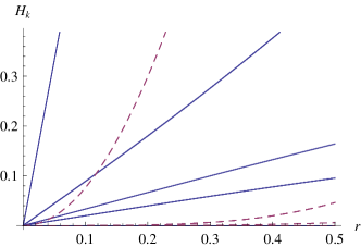
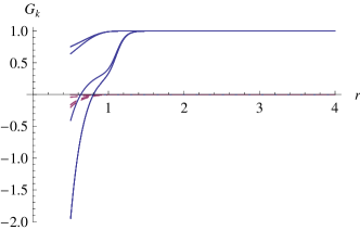
Figure 1: Eigenvalues of the matrices $\hat{G}_{k}(r)$ and $\hat{H}_{k}(r)$ for $k=1$, truncated at $j_{\hbox{\tiny max}}=2$, using the dielectric function in Eq. (52) with $h=4$, $w=1$, and $s=8$. For each eigenvalue, solid lines show the real part and dashed lines show the imaginary part. Taking $r_{0}=\frac{1}{2}$, we only calculate $\hat{H}_{k}(r)$ for $r<r_{0}$ and $\hat{G}_{k}(r)$ for $r>r_{0}$.

For comparison, we can reconstruct the normalized physical wavefunction $\hat{\psi}_{k}^{\hbox{\tiny norm}}(r)$ from these results by writing

$$\hat{\psi}_{k}^{\hbox{\tiny norm}}(r)=\frac{1}{\sqrt{2\pi}}\cdot\left\{\begin{array}[]{cc}\hat{G}_{-k}(r)\hat{W}(-kr)\hat{P}\left(\widetilde{\cal W}_{-k}\right|_{r=r_{0}}\hat{P}-\hat{G}_{k}(r)\hat{W}(kr)\hat{P}\left(\widetilde{\cal W}_{k}\right|_{r=r_{0}}\hat{P}&\hbox{~{}~{}for $r>r_{0}$}\cr\hat{W}(kr)^{-1}\hat{H}_{k}(r)\hat{C}_{k}&\hbox{~{}~{}for $r<r_{0}$}\end{array}\right.,$$ (53)

where $\hat{P}$ is the projection matrix onto the transverse modes, the modified Wronskian $\widetilde{\cal W}_{k}$ is evaluated at $r=r_{0}$ using Eqs. (47) and (20), and $\hat{C}_{k}$ is a constant matrix that matches the normalization of the two solutions, which is obtained by setting the two expressions in Eq. (53) equal at $r=r_{0}$. This result, shown in Fig. 2, displays the typical oscillations associated with wave number $k$. By “factoring out” the free contribution $\hat{W}(kr)$, our method allows us to avoid these oscillations in numerical calculations.

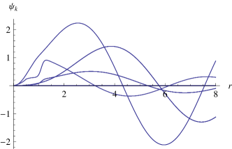
Figure 2: Eigenvalues of the matrix $\hat{\psi}_{k}^{\hbox{\tiny norm}}(r)$ for $k=1$, truncated at $j_{\hbox{\tiny max}}=2$, using the dielectric function in Eq. (52) with $h=4$, $w=1$, and $s=8$. The two expressions in Eq. (53) join smoothly at $r_{0}=\frac{1}{2}$.

To illustrate the $S$-matrix as a function of $k$, we consider a dielectric with a Drude model dependence on wave number,

$$\epsilon_{\ell m}(r)=\sqrt{4\pi}\,\delta_{\ell 0}\delta_{m0}+\frac{(2\pi)^{2}}{\frac{\pi}{\sigma_{p}}\sqrt{-k^{2}}-(\lambda_{p}k)^{2}}p_{\ell m}(r)\,,$$ (54)

where $p_{\ell m}(r)$ specifies the radial profile function for each spherical component of the dielectric profile. Here $\lambda_{p}$ is the plasma wavelength, $\sigma_{p}$ is the conductivity, and the frequency is $\omega=c\sqrt{k^{2}}$. We consider a deformed sphere using a profile given by

$$p_{00}(r)=\sqrt{4\pi}\frac{1-\tanh\left[s(r-w)\right]}{2}\hbox{\qquad and \qquad}p_{10}(r)=\frac{1-\tanh\left[s(r-w)\right]}{2}\,,$$ (55)

with all other $p_{\ell m}(r)$ equal to zero. The $j=1$ eigenphase shifts for this case, given by one-half of the argument of the eigenvalues of the $S$-matrix, are shown in Fig. 3 as functions of $k$. By comparing to the case where $\epsilon_{00}(r)$ is kept the same but $\epsilon_{10}(r)$ is set to zero, we see that a nontrivial $\epsilon_{10}(r)$ mixes the polarization channels and splits the degeneracy between $|m|=1$ and $m=0$. As expected, these effects vanish at small $k$, where modes have wavelengths much larger than the length scale associated with the asymmetry, and also at large $k$, where modes have wavelengths much smaller than the plasma wavelength.

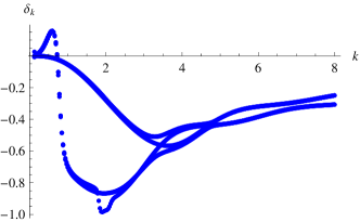
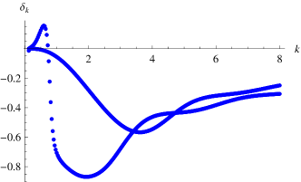
Figure 3: Eigenphase shifts, given by one-half the argument of the eigenvalues of the $S$-matrix, truncated at $j_{\hbox{\tiny max}}=1$. The left panel shows the case of the dielectric function given by Eqs. (54) and (55), with $\lambda_{p}=\pi$, $\sigma_{p}=1$, $w=1$, and $s=8$, while the right panel shows the result for the same $\epsilon_{00}(r)$, but with $\epsilon_{10}(r)=0$.

V Discussion and Future Developments

We have developed a variable phase method to calculate the scattering $S$-matrix for potentials in quantum mechanics and dielectrics in electromagnetism that are localized but do not have any particular symmetries. The result takes the form of a matrix initial value ODE given in terms of a spherical harmonic decomposition of the scattering source. By using the Wronskian, we can combine inward and outward integration in $r$ to obtain a well-behaved numerical computation, which remains tractable even for imaginary wave number $k$. Finally, we have extended this approach to the electromagnetic case by considering a modification of the Maxwell wave equation that avoids problems associated with disentangling the transverse and longitudinal waves.

Our high-level Mathematica code provides a transparent and flexible high-level implementation of the methods described here, but it is only suitable for small- to moderate-scale calculations. Larger-scale calculations involving large numbers of partial waves will require the use of optimized low-level parallel linear algebra routines. Since the ultimate problem to be solved is quite generic, such calculations can take advantage of standard numerical packages for matrix ODEs.

VI Acknowledgements

N. G. thanks G. Bimonte, J. Dunham, T. Emig, R. L. Jaffe, M. Kardar, M. Krüger, M. Maghrebi, M. Quandt, H. Reid, and H. Weigel for helpful conversations, suggestions, and references. A. F. and N. G. were supported in part by the National Science Foundation (NSF) through grants PHY-0855426 and PHY-1213456.

Appendix A Differential Operators

Here we collect the differential operator relations needed to express Eq. (37) in the vector spherical harmonic basis, taken from Ref. Varshalovich et al. (1988). In these equations $f(r)$ is an arbitrary radial function, $Y_{j}^{m}(\theta,\phi)$ is an ordinary spherical harmonic, and $\bm{Y}^{\ell}_{jm}(\theta,\phi)$ is a vector spherical harmonic.

$$\nabla\left(f(r)Y_{j}^{m}(\theta,\phi)\right) = \sqrt{\frac{j}{2j+1}}\left(\frac{d}{dr}+\frac{j+1}{r}\right)f(r)\bm{Y}^{\ell=j-1}_{jm}(\theta,\phi)-\sqrt{\frac{j+1}{2j+1}}\left(\frac{d}{dr}-\frac{j}{r}\right)f(r)\bm{Y}^{\ell=j+1}_{jm}(\theta,\phi)$$ (56)

$$\nabla\cdot\left(f(r)\bm{Y}^{\ell=j+1}_{jm}(\theta,\phi)\right) = -\sqrt{\frac{j+1}{2j+1}}\left(\frac{d}{dr}+\frac{j+2}{r}\right)f(r)Y_{j}^{m}(\theta,\phi)$$ (57)

$$\nabla\cdot\left(f(r)\bm{Y}^{\ell=j}_{jm}(\theta,\phi)\right) = 0$$ (58)

$$\nabla\cdot\left(f(r)\bm{Y}^{\ell=j-1}_{jm}(\theta,\phi)\right) = \sqrt{\frac{j}{2j+1}}\left(\frac{d}{dr}-\frac{j-1}{r}\right)f(r)Y_{j}^{m}(\theta,\phi)$$ (59)

$$\nabla\times\left(f(r)\bm{Y}^{\ell=j+1}_{jm}(\theta,\phi)\right) = i\sqrt{\frac{j}{2j+1}}\left(\frac{d}{dr}+\frac{j+2}{r}\right)f(r)\bm{Y}^{\ell=j}_{jm}(\theta,\phi)$$ (60)

$$\nabla\times\left(f(r)\bm{Y}^{\ell=j}_{jm}(\theta,\phi)\right) = i\sqrt{\frac{j}{2j+1}}\left(\frac{d}{dr}-\frac{j}{r}\right)f(r)\bm{Y}^{\ell=j+1}_{jm}(\theta,\phi)+i\sqrt{\frac{j+1}{2j+1}}\left(\frac{d}{dr}+\frac{j+1}{r}\right)f(r)\bm{Y}^{\ell=j-1}_{jm}(\theta,\phi)$$ (61)

$$\nabla\times\left(f(r)\bm{Y}^{\ell=j-1}_{jm}(\theta,\phi)\right) = i\sqrt{\frac{j+1}{2j+1}}\left(\frac{d}{dr}-\frac{j-1}{r}\right)f(r)\bm{Y}^{\ell=j}_{jm}(\theta,\phi)$$ (62)

Appendix B Free Green’s Functions and Plane Wave Expansions

Throughout this paper we have considered scattering in a spherical partial wave basis. For both Casimir calculations and traditional scattering problems, it is helpful to be able to convert these results to a plane wave basis. The key tools in this conversion are the expansion of a plane wave and the expansion of the free Green’s function in terms of free spherical waves. Again drawing on Ref. Varshalovich et al. (1988), we collect those expansions here. For scalar scattering we have the well-known results

$$e^{i\bm{k}\cdot\bm{r}}=4\pi\sum_{\ell m}i^{\ell}j_{\ell}(kr)Y_{\ell}^{m}(\theta_{k},\phi_{k})^{\ast}Y_{\ell}^{m}(\theta,\phi)\,,$$ (63)

where $\theta_{k}$ and $\phi_{k}$ are the angles of $\hat{\bm{k}}$ in spherical coordinates, and

$${\cal G}_{0}(\bm{r},\bm{r^{\prime}},k)=ik\sum_{\ell m}j_{\ell}(kr_{<})h^{(1)}_{\ell}(kr_{>})Y_{\ell}^{m}(\theta^{\prime},\phi^{\prime})^{\ast}Y_{\ell}^{m}(\theta,\phi)\,,$$ (64)

where $r_{<}$ ($r_{>}$) is the smaller (larger) of $r=|\bm{r}|$ and $r^{\prime}=|\bm{r}^{\prime}|$. For vector waves, the expansion of a plane wave with polarization $\bm{\xi}$ becomes

$$\bm{\xi}e^{i\bm{k}\cdot\bm{r}}=4\pi\sum_{\ell jm}i^{\ell}\left(\bm{\xi}\cdot\bm{Y}^{\ell}_{jm}(\theta_{k},\phi_{k})^{\ast}\right)j_{\ell}(kr)\bm{Y}^{\ell}_{jm}(\theta,\phi)\,,$$ (65)

while the expansion of the free dyadic Green’s function is

$$\mathbb{G}(\bm{r}_{1},\bm{r}_{2},k)=ik\sum_{\ell jm}j_{\ell}(kr_{<})h^{(1)}_{\ell}(kr_{>})\bm{Y}^{\ell}_{jm}(\theta_{1},\phi_{1})^{\ast}\otimes\bm{Y}^{\ell}_{jm}(\theta_{2},\phi_{2})\,.$$ (66)

We can also express these results in terms of transverse and longitudinal vector spherical harmonics. For the decomposition of a vector plane wave, we define

$$\bm{Y}^{M}_{jm}(\theta,\phi) = \bm{Y}^{\ell=j}_{jm}(\theta,\phi)$$ (67)

$$\bm{Y}^{N}_{jm}(\theta,\phi) = \sqrt{\frac{j+1}{2j+1}}\bm{Y}^{\ell=j-1}_{jm}(\theta,\phi)+\sqrt{\frac{j}{2j+1}}\bm{Y}^{\ell=j+1}_{jm}(\theta,\phi)\,,$$ (68)

for $j=1,2,3\ldots$, and

$$\bm{Y}^{L}_{jm}(\theta,\phi)=\sqrt{\frac{j}{2j+1}}\bm{Y}^{\ell=j-1}_{jm}(\theta,\phi)-\sqrt{\frac{j+1}{2j+1}}\bm{Y}^{\ell=j+1}_{jm}(\theta,\phi)$$ (69)

where $j=0,1,2,3\ldots$. (Note that for $j=0$, the unphysical term with $\ell=-1$ is multiplied by zero.) Similarly, we consider the free transverse modes in Eqs. (43) along with the free longitudinal mode, given by

$$\bm{L}_{jm,k}(r,\theta,\phi)=\sqrt{\frac{j}{2j+1}}z_{j-1}(kr)\bm{Y}^{\ell=j-1}_{jm}(\theta,\phi)+\sqrt{\frac{j+1}{2j+1}}z_{j+1}(kr)\bm{Y}^{\ell=j+1}_{jm}(\theta,\phi)$$ (70)

for $j=0,1,2\ldots$.

For the decomposition of a plane wave, we then have

$$\bm{\xi}e^{i\bm{k}\cdot\bm{r}}=4\pi\sum_{\bm{\chi}jm}i^{j+\sigma}\left(\bm{\xi}\cdot\bm{Y}^{\chi}_{jm}(\theta_{k},\phi_{k})^{\ast}\right)\bm{\chi}^{\rm reg}_{jm,k}(r,\theta,\phi)\,,$$ (71)

where $\sigma=0,1,-1$ for $\bm{\chi}=\bm{M},\bm{N},\bm{L}$ respectively, and for the free dyadic Green’s function we have

$$\mathbb{G}(\bm{r}_{1},\bm{r}_{2},k)=ik\sum_{\bm{\chi}jm}\bm{\chi}^{\rm reg}_{jm,k}(\bm{r}_{<})^{\ast}\otimes\bm{\chi}^{\rm out}_{jm,k}(\bm{r}_{>})\,.$$ (72)

again for $\bm{\chi}=\bm{M},\bm{N},\bm{L}$. Here the regular solution is given by taking $z_{\ell}(kr)=j_{\ell}(kr)$ in Eqs. (43) and (70), while the outgoing solution has $z_{\ell}(kr)=h^{(1)}_{\ell}(kr)$.

References

- Newton (1966) R. G. Newton, Scattering Theory of Waves and Particles (McGraw-Hill, New York, 1966).
- Chadan and Sabatier (1989) K. Chadan and P. Sabatier, Inverse Problems in Quantum Scattering Theory (Springer-Verlag, Berlin, 1989).
- Kats (1977) E. I. Kats, Sov. Phys. JETP 46, 109 (1977).
- Jaekel and Reynaud (1991) M. T. Jaekel and S. Reynaud, J. Physique I 1, 1395 (1991).
- Emig et al. (2007) T. Emig, N. Graham, R. L. Jaffe, and M. Kardar, Phys. Rev. Lett. 99, 170403 (2007).
- Emig et al. (2008) T. Emig, N. Graham, R. L. Jaffe, and M. Kardar, Phys. Rev. D77, 025005 (2008).
- Rahi et al. (2009) S. J. Rahi, T. Emig, N. Graham, R. L. Jaffe, and M. Kardar, Phys. Rev. D80, 085021 (2009).
- Kenneth and Klich (2006) O. Kenneth and I. Klich, Phys. Rev. Lett. 97, 160401 (2006).
- Graham et al. (2009) N. Graham, M. Quandt, and H. Weigel, Spectral Methods in Quantum Field Theory (Springer-Verlag, Berlin, 2009).
- Waterman (1965) P. C. Waterman, Proceedings of the IEEE 53, 805 (1965).
- Waterman (1971) P. C. Waterman, Phys. Rev. D 3, 825 (1971).
- Mishchenkoa et al. (2004) M. I. Mishchenkoa, G. Videenb, V. A. Babenkoc, N. G. Khlebtsovd, and T. Wriedte, J. of Quantitative Spectroscopy & Radiative Transfer 88, 357 (2004).
- Calogero (1967) F. Calogero, Variable Phase Approach to Potential Scattering (Academic Press, New York, 1967).
- Reid et al. (2009) M. T. H. Reid, A. W. Rodriguez, J. White, and S. G. Johnson, Phys. Rev. Lett. 103, 040401 (2009).
- Johnson (1999) B. R. Johnson, J. Opt. Soc. Am. A 16, 845 (1999).
- Press et al. (1992) W. H. Press, S. A. Teukolsky, W. T. Vetterling, and B. P. Flannery, Numerical Recipes in C: The Art of Scientific Computing, 2nd edition (Cambridge University Press, Cambridge, 1992).
- Graham et al. (2002) N. Graham, R. L. Jaffe, V. Khemani, M. Quandt, M. Scandurra, and H. Weigel, Nucl. Phys. B645, 49 (2002).
- Varshalovich et al. (1988) D. Varshalovich, A. Moskalev, and V. Khersonsky, Quantum Theory of Angular Momentum: Irreducible Tensors, Spherical Harmonics, Vector Coupling Coefficients, 3-j Symbols (World Scientific, Hackensack, NJ, 1988).
- Biedenharn and Louck (2009) L. C. Biedenharn and J. D. Louck, Angular Momentum in Quantum Physics: Theory and Application (Encyclopedia of Mathematics and its Applications) (Cambridge University Press, Cambridge, 2009).