Dynamical Eigenmodes of Star and Tadpole Polymers

Abstract

The dynamics of phantom bead-spring chains with the topology of a symmetric star with $f$ arms and tadpoles ($f=3$, a special case) is studied, in the overdamped limit. In the simplified case where the hydrodynamic radius of the central monomer is $f$ times as heavy as the other beads, we determine their dynamical eigenmodes exactly, along the lines of the Rouse modes for linear bead-spring chains. These eigenmodes allow full analytical calculations of virtually any dynamical quantity. As examples we determine the radius of gyration, the mean square displacement of a tagged monomer, and, for star polymers, the autocorrelation function of the vector that spans from the center of the star to a bead on one of the arms.

I Introduction

Bead-spring models play a central role in the theory and modelling of polymer dynamics. Most of the applications of bead-spring models (and polymer dynamics in general) is found for linear polymers, for which the polymer consists of a linear sequence of beads connected by harmonic springs. For a linear bead-spring polymer chain, with position ${\bf R}_{n}$ of the $n$-th bead, $n=0\dots N$, the potential energy is thus

$$U=\frac{k}{2}\sum_{n=1}^{N}\left({\bf R}_{n}-{\bf R}_{n-1}\right)^{2},$$ (1)

in which $k$ is the spring constant. Besides the heavily studied linear polymer chains there are many other types of polymers whose dynamics deserve closer inspection. In this paper we concern ourselves with the dynamics of bead-spring chains that have the topology of a symmetric star (with $f$ arms) and tadpoles.

Further, in the context of bead-spring models, the Rouse model for linear phantom chains rouse deserves a special mention. In the Rouse model the dynamics of the beads is formulated in the overdamped limit, with a solvent with viscous drag coefficient $\zeta$, and with thermal forces ${\bf g}_{n}$ on the $n$-th bead, such that the dynamical equations of motion become

$$\frac{d{\bf R}_{n}}{dt}=-\frac{1}{\zeta}\frac{\partial U}{\partial{\bf R}_{n}}+{\bf g}_{n}.$$ (2)

Here, the thermal forces are delta-correlated, namely

$$\left<{\bf g}_{i}(t)\cdot{\bf g}_{j}(t^{\prime})\right>=\frac{6k_{B}T}{\zeta}\delta_{ij}\delta(t-t^{\prime}),$$ (3)

with Boltzmann constant $k_{B}$ and temperature $T$.

The reason why, to date, the Rouse model deserves a special mention, lies in the fact that it allows full analytical calculations of virtually any dynamical quantity. Rather than the equations of motion for the individual beads, one considers the so-called Rouse modes, whose amplitudes at time $t$ are given by

$${\bf X}_{p}(t)=\frac{1}{N+1}\sum_{n=0}^{N}\cos\left[\frac{\pi(n+1/2)p}{N+1}\right]\,{\bf R}_{n}(t),$$ (4)

with $p=0\dots N$. The dynamics of these modes are uncorrelated, and one can derive the following relation for $p,q\neq 0$ exactly doi ; de from the equation of motion (2):

$$X_{pq}(t)\equiv\langle{\bf X}_{p}(t)\cdot{\bf X}_{q}(0)\rangle=A_{1}\frac{N}{p^{2}}\,\exp\left[-A_{2}\,\frac{p^{2}}{N^{2}}\,t\right]\,\delta_{pq},$$ (5)

where $A_{1}=3k_{B}T/(2\pi^{2}k)$ and $A_{2}=\pi^{2}k/\zeta$. Here, and all throughout this paper, the angular brackets represent an average over the equilibrium ensemble of polymer chains. Equation (5) is further supplemented by $X_{0p}(t)=0$ for $p\neq 0$, and $X_{00}(t)\equiv\langle[{\bf X}_{0}(t)-{\bf X}_{0}(0)]^{2}\rangle=6k_{B}Tt/(\zeta N)$, where ${\bf X}_{0}(t)$ is the location of the center-of-mass of the polymer at time $t$. Using these mode amplitude correlation functions, the quantities of interest for a phantom chain can be analytically tracked by reconstructing them from the modes doi ; de .

Using the definition of Rouse modes it has been shown in recent works that the dynamics of a tagged bead in a linear bead-spring model is described by the Generalized Langevin Equation (GLE) jstat1 ; jstat2 , and that the dynamics of polymers with steric repulsion (also known as self-avoiding polymer chains) saw-rouse , as well as of those in melts as described by the repton model reptonmodes can be well-approximated. Here, we continue this line of research, but now we are interested in exact solutions of the dynamical properties of polymers with the topology of stars and tadpoles.

The structure of this paper is as follows. In Sec. II we present the dynamical eigenmodes of symmetric phantom star polymers, and use the mode amplitudes to provide analytical expressions to the radius of gyration, mean square displacement of a tagged monomer, and the autocorrelation function of the vector that spans from the center of the star to a bead on one of the arms. In Sec. III we repeat the exercise for chains with tadpole topology. We end the paper with a short discussion in Sec. IV.

II Dynamical eigenmodes of symmetric star polymers

A major difficulty for dynamics of polymers with a more complex topology like the symmetric star polymer is that in most cases an elegant analytical expression for the set of dynamical eigenmodes cannot be found starthesis . Here we show that for a symmetric star polymer with a special central bead the dynamical eigenmodes can indeed be written down exactly, and subsequently the dynamical behavior of many interesting physical quantities can be determined precisely. For simplicity, in commensuration with the Rouse model, henceforth we term these dynamical eigenmodes as Rouse modes. Specifically, we consider a star polymer with $f$ identical arms, each consisting of $N$ identical beads, connected to a central bead whose hydrodynamic radius is $f$ times as big as the other ones, i.e., its viscous drag is $f$ times as large. A graphical representation of such a star polymer with $f=5$ and $N=4$ can be found in Fig. 1. It is worthwhile to note in this context that a key method to synthesize a star polymer chain is to attach the arms, which are linear chains, to a multivalent central core with sticky ends (see, e.g., Ref. gao and the references cited therein). Although from the synthesis process it is realistic that the core has a significantly higher hydrodynamic radius, the choice in our simplified model to make hydrodynamic radius of the central bead exactly $f$ times as the other beads is motivated by our strive to determine the Rouse modes exactly. For modestly-sized chains, where the hydrodynamic radius of the core is not $f$ times as big as the arm beads, the dynamical matrix (the homogenous part of the dynamical differential equation) has been diagonalized numerically, yielding the numerical identification of the Rouse modes starthesis .

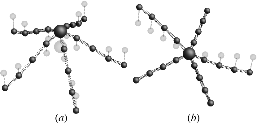
Figure 1: Two graphical representations of a symmetrical star polymer to visualize the Rouse modes. Depicted is a symmetric starpolymer with five arms consisting of four beads each and a central monomer which has a friction coefficient five times that of beads in the arms. The transparent configurations are polymers in the origin stretched in the $xy$-plane for visual convenience with no Rouse mode excited in the $z$-direction. The opague configurations are like the transparent ones but with a pure ${\bf X}_{1}$ mode (a) and ${\bf Y}_{1}^{(i,j)}$ modes (b) in the z-direction.

We label the position of the central bead as ${\bf R}_{0}$ and let ${\bf R}_{a,n}$ be the position of the $n$-th bead, $n=1\dots N$, in the $a$-th arm, $a=1\dots f$. We consider two types of Rouse modes given by

$${\bf X}_{p}(t) = \frac{1}{N+1}\left\{\cos\left[\frac{\pi p/2}{N+1}\right]{\bf R}_{0}(t)+\frac{1}{f}\sum_{a,n=1}^{f,N}\cos\left[\frac{\pi(n+1/2)p}{N+1}\right]{\bf R}_{a,n}(t)\right\},$$ (6a)

$${\bf Y}_{q}^{(i,j)}(t) = \frac{1}{2N+1}\sum_{n=1}^{N}\cos\left[\frac{\pi(N-n+1/2)(q-1/2)}{N+1/2}\right]\left({\bf R}_{i,n}(t)-{\bf R}_{j,n}(t)\right),$$ (6b)

with $p=0\dots N$ and $q=1\dots N$. A visualization of the two kinds of modes can also be found in Fig. 1. The first set of modes ${\bf X}_{p}(t)$ are like Rouse modes for a stringpolymer through all the arms. The second set of modes ${\bf Y}_{p}^{(i,j)}(t)$ can also be thought of as Rouse modes as in Eq. (4) with $p$ odd valued and through a linear chain of length $2N+1$ made up by arms $i$ and $j$ and the central bead. There are $Nf(f-1)/2$ modes of the type ${\bf Y}_{p}^{(i,j)}(t)$ with $i<j$, but the total set of these modes contain only $(f-1)N$ independent degrees of freedom, for instance because ${\bf Y}_{p}^{(i,k)}(t)$=${\bf Y}_{p}^{(i,j)}(t)$+${\bf Y}_{p}^{(j,k)}(t)$; we could have constructed, for every $p$, an orthogonal set of $f-1$ modes out of the full set of modes ${\bf Y}_{p}^{(i,j)}(t)$, but we choose not to do that for the sake of mathematical elegance. Combined with $N+1$ modes ${\bf X}_{p}(t)$, the total set contains $fN+1$ three-dimensional modes needed to describe the system that has $fN+1$ beads so that the number of degrees of freedom is the same.

Similarly to the single chain, the dynamics of these modes for a star polymer with long arms are captured by

$$X_{pq}(t) \equiv \langle{\bf X}_{p}(t)\cdot{\bf X}_{q}(0)\rangle=\frac{3k_{b}T}{2\pi^{2}k}\frac{N}{fp^{2}}\,\exp\left[-\frac{\pi^{2}k}{\zeta}\,\frac{p^{2}}{N^{2}}\,t\right]\,\delta_{pq},$$ (7a)

$$Y_{pq}^{(i,j)(k,l)}(t) \equiv \langle{\bf Y}_{p}^{(i,j)}(t)\cdot{\bf Y}_{q}^{(k,l)}(0)\rangle$$ (7b)

$$= \frac{3k_{b}T}{8\pi^{2}k}\frac{N}{(p-1/2)^{2}}\,\exp\left[-\frac{\pi^{2}k}{\zeta}\frac{(p-1/2)^{2}}{N^{2}}t\right]\delta_{pq}\delta_{(i,j)(k,l)},$$

where $\delta_{(i,j)(k,l)}=\delta_{ik}-\delta_{jk}-\delta_{il}+\delta_{jl}$. This is supplemented by $X_{00}(t)\equiv\langle[{\bf X}_{0}(t)-{\bf X}_{0}(0)]^{2}\rangle=6k_{B}Tt/(\zeta f(N+1))$ and all other correlations between modes strictly zero. The derivations of the Rouse mode amplitudes can be found in Appendix A.

II.1 Radius of gyration

The squared radius of gyration is defined as the weighted sum over all differences between the position of a monomer and the center of mass squared. Below we work out the radius of gyration for the case of the star polymer where the central monomer is $f$ times heavier than the other beads, although the radius of gyration can be calculated following the same line for other cases as well. In the former case the location of the center-of-mass ${\bf R}_{cm}(t)\equiv{\bf X}_{0}(t)$, and the squared radius of gyration is defined as

$$R_{g}^{2}=\frac{1}{f(N+1)}\left[f\langle[{\bf R}_{0}(t)-{\bf R}_{cm}(t)]^{2}\rangle+\sum_{i,n=1}^{f,N}\langle[{\bf R}_{i,n}(t)-{\bf R}_{cm}(t)]^{2}\rangle\right],$$ (8)

which can be calculated by plugging in Eq. (34). This reduces to

$$R_{g}^{2}=2\sum_{p=1}^{N}X_{pp}(0)+\frac{4(2N+1)}{f^{3}(N+1)}\sum_{p,i,j,k=1}^{N,f,f,f}Y_{pp}^{(i,j)(i,k)}(0).$$ (9)

Plugging in Eq. (7) explicitly and taking the long polymer limit yields

$$R_{g}^{2}=\frac{3k_{B}T}{k\pi^{2}}\frac{N}{f}\sum_{p=1}^{\infty}\frac{1}{p^{2}}+\frac{3k_{B}T}{k\pi^{2}}\frac{N}{f^{3}}\sum_{i,j,k=1}^{f,f,f}\delta_{(i,j)(i,k)}\sum_{p=1}^{\infty}\frac{1}{(p-1/2)^{2}}.$$ (10)

The sums can be evaluated by using Eq. (47).

And so the radius of gyration squared for a long symmetric star polymer becomes

$$R_{g}^{2} =\frac{k_{B}TN}{k}\frac{3f-2}{2f}.$$ (11)

This result is consistent with that of a linear chain ($f=1$).

II.2 Mean square displacement of a monomer

We now consider the mean square displacement of the central bead and a bead in an arm for a star polymer with long arms. We start by defining the displacement vector for the central bead and writing it in terms of modes using Eq. (34a):

$$\Delta{\bf R}_{0}(t)\equiv {\bf R}_{0}(t)-{\bf R}_{0}(0)$$

$$= {\bf X}_{0}(t)-{\bf X}_{0}(0)+2\sum_{p=1}^{N}\cos\left[\frac{\pi p/2}{N+1}\right]\left\{{\bf X}_{p}(t)-{\bf X}_{p}(0)\right\}.$$ (12)

The mean square displacement is then given by

$$\langle\Delta{\bf R}_{0}^{2}(t)\rangle=X_{00}(t)+8\sum_{p=1}^{N}\cos^{2}\left[\frac{\pi p/2}{N+1}\right]\{X_{pp}(0)-X_{pp}(t)\},$$ (13)

where Eq. (7a) can be plugged in, and the orthogonality of the modes was already used for simplification. Before doing so, let us look at very short time scales $t<\zeta/(4k)$. The exponent in $X_{pq}(t)$ can then be expanded and the sum exactly evaluated using Eq. (45a), resulting in $\langle\Delta{\bf R}_{0}^{2}(t)\rangle=6k_{B}Tt/(\zeta f)$ dominating over the mean square displacement of the whole polymer which at short time scales is negligible. At very long time scales $X_{pq}(t)$ goes to zero and the term with the summation in Eq. (13) can again be exactly evaluated using Eq. (46a). So for $t<\zeta N^{2}/(3k)$ the summation has a larger contribution than the mean square displacement of the whole polymer. For intermediate times the summation dominates and can be rewritten as an integral for very long polymers:

$$\langle\Delta{\bf R}_{0}^{2}(t)\rangle=\frac{12k_{B}T}{\pi^{2}kf}\int_{0}^{\infty}\frac{dx}{x^{2}}\left\{1-\exp\left[-\frac{k\pi^{2}t}{\zeta}x^{2}\right]\right\}=\frac{12k_{B}T}{f}\sqrt{\frac{t}{\pi k\zeta}}.$$ (14)

The mean square displacement as approximated for intermediate times is greater than that of the approximation for the short time scales for $t>4\zeta/(\pi k)$, so that is when the intermediate time regime begins. For the central bead in a star polymer the mean square displacement then becomes

$$\langle\Delta{\bf R}_{0}^{2}(t)\rangle=\left\{\begin{array}[]{ll}\displaystyle{\frac{6k_{B}T}{\zeta f}t,\quad\quad\quad\quad\quad\mbox{for}\,t<\frac{\zeta}{4k}}\\ \displaystyle{\frac{12k_{B}T}{f}\sqrt{\frac{t}{\pi k\zeta}},\quad\quad\mbox{for}\,\frac{4\zeta}{\pi k}<t<\frac{N^{2}\zeta}{3k}}\\ \displaystyle{\frac{6k_{B}T}{\zeta f(N+1)}t,\quad\quad\quad\quad\quad\mbox{for}\,t>\frac{N^{2}\zeta}{3k}}\end{array}\right..$$ (15)

Figure 2 shows the exact evaluation of Eq. (13) for some star polymer together with approximations made for the short, intermediate and long time scales found in Eq. (15). The central bead first behaves like a single bead with friction coefficient $\zeta f$. After that the movement is restricted by local connections to surrounding beads in the polymer. For very long times the position of the bead within the polymer is negligible and the mean square displacement behaves as that of a single bead with friction coefficient $\zeta f(N+1)$.

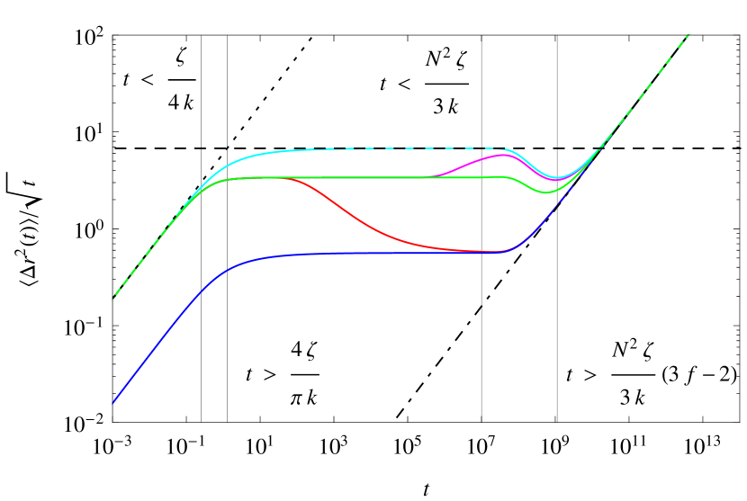
Figure 2: The scaled mean square displacement $\langle\Delta{\bf R}^{2}(t)\rangle/\sqrt{t}$ as a function of time. The mean square displacement of several beads in a symmetric star polymer as given by Eqs. (13,17) were exactly evaluated with $A=12$ and $N=10^{4}$ and other parameters put to $1$. The solid blue line corresponds to the mean square displacement of the central bead whereas the red, green, magenta, and cyan solid lines correspond to $n=10^{-3}N,N/2,9N/10$, and $N$ in Eq. (17) respectively. A bead positioned somewhere along the arm will at first behave as if it were in the middle of the arm. After time grows either the end or the center will become an influence at first and the bead will start mimicking a bead at one of those places. The short time scale $t<\zeta/(4k)$ and the very long time scale $t\gg N^{2}\zeta(3f-2)/(3k)$ for which $\langle\Delta{\bf R}^{2}(t)\rangle\sim t$ corresponding to the dotted and dot-dashed lines are separated by a time during which $\langle\Delta{\bf R}^{2}(t)\rangle\sim\sqrt{t}$ corresponding to the dashed line as in agreement with Eqs. (15,19-20).

A very similar approach can be used for the mean square displacement of a bead in an arm of the star polymer, defined as

$$\Delta{\bf R}_{n}(t)\equiv {\bf R}_{i,n}(t)-{\bf R}_{i,n}(0)$$

$$= {\bf X}_{0}(t)-{\bf X}_{0}(0)+2\sum_{p=1}^{N}\cos\left[\frac{\pi(n+1/2)p}{N+1}\right]\{{\bf X}_{p}(t)-{\bf X}_{p}(0)\}$$

$$+\frac{4}{f}\sum_{j,p=1}^{f,N}\cos\left[\frac{\pi(N-n+1/2)(p-1/2)}{N+1/2}\right]\{{\bf Y}^{(i,j)}_{p}(t)-{\bf Y}^{(i,j)}_{p}(0)\}.$$ (16)

Using orthogonality of mode ${\bf Y}^{(i,j)}_{p}$ with ${\bf X}_{q}$ and with ${\bf Y}^{(k,l)}_{q}$ with $q\neq p$, and evaluating the double sum over the arms, the mean square displacement becomes

$$\langle\Delta{\bf R}_{n}^{2}(t)\rangle= X_{00}(t)+8\sum_{p=1}^{N}\cos^{2}\left[\frac{\pi(n+1/2)p}{N+1}\right]\left\{X_{pp}(0)-X_{pp}(t)\right\}$$

$$+\frac{16(f-1)}{f}\sum_{p=1}^{N}\cos^{2}\left[\frac{\pi(N-n+1/2)(p-1/2)}{N+1/2}\right]$$

$$\times\left\{Y_{pp}^{(1,2)(1,2)}(0)-Y_{pp}^{(1,2)(1,2)}(t)\right\}.$$ (17)

For small values of $t$ the exponents can again be expanded and the sum exactly evaluated using Eqs. (45a-45b) so that in the long polymer limit $\langle\Delta{\bf R}_{n}^{2}(t)\rangle=6k_{B}Tt/\zeta$. The summation reaches its maximum, using Eqs. (46a-46b), on long time scales so that for a bead at the end of an arm the mean square displacement term of the whole polymer will start to dominate for $t>N^{2}\zeta(3f-2)/(3k)$. The closer a bead is to the central bead the faster its mean square displacement will behave like that of the whole polymer. We can again approximate the summation by an integral for intermediate times but depending on the position of the bead in an arm it will behave differently.

$$\langle\Delta{\bf R}_{n}^{2}(t)\rangle= \frac{12k_{B}T}{\pi^{2}kf}\int_{0}^{\infty}\frac{dx}{x^{2}}\left\{1-\exp\left[-\frac{k\pi^{2}t}{\zeta}x^{2}\right]\right\}$$

$$\times\left\{\cos\left[\frac{\pi(n+1/2)p}{N+1}\right]+(f-1)\cos\left[\frac{\pi(N-n+1/2)(p-1/2)}{N+1/2}\right]\right\}$$ (18)

The exponent in the integral will suppress the contribution for higher $p$-values. For a bead at the end of an arm, $n$ equals $N$, the cosines can be taken to be $1$ and the integral as the same as the integral for the central bead but with an extra factor $f$. For a bead in the middle of an arm, $n$ equals $N/2$, in the long polymer limit the first cosine will be $1$ for even values of $p$ and $0$ for odd values, and the second cosine will be $1/2$ for all values of $p$. This will give the same integral as for the bead at the end of an arm but smaller by a factor $1/2$. We thus find for the mean square displacement of a bead at the end of an arm

$$\langle\Delta{\bf R}_{N}^{2}(t)\rangle=\left\{\begin{array}[]{ll}\displaystyle{\frac{6k_{B}T}{\zeta}t,\quad\quad\quad\quad\quad\mbox{for}\,t<\frac{\zeta}{4k}}\\ \displaystyle{12k_{B}T\sqrt{\frac{t}{\pi k\zeta}},\quad\quad\mbox{for}\,\frac{4\zeta}{\pi k}<t<\frac{N^{2}\zeta}{3k}}\\ \displaystyle{\frac{6k_{B}T}{\zeta fN}t,\quad\quad\quad\quad\quad\mbox{for}\,t>\frac{N^{2}\zeta}{3k}(3f-2)}\end{array}\right..$$ (19)

For the bead located exactly in the middle of an arm the mean square displacement becomes

$$\langle\Delta{\bf R}_{N/2}^{2}(t)\rangle=\left\{\begin{array}[]{ll}\displaystyle{\frac{6k_{B}T}{\zeta}t,\quad\quad\quad\quad\quad\mbox{for}\,t<\frac{\zeta}{4k}}\\ \displaystyle{6k_{B}T\sqrt{\frac{t}{\pi k\zeta}},\quad\quad\,\,\,\,\mbox{for}\,\frac{4\zeta}{\pi k}<t<\frac{N^{2}\zeta}{3k}}\\ \displaystyle{\frac{6k_{B}T}{\zeta fN}t,\quad\quad\quad\quad\quad\mbox{for}\,t>\frac{N^{2}\zeta}{3k}(3f-2)}\end{array}\right..$$ (20)

Figure 2 shows the exact evaluation of Eq. (17) and demonstrates the validity of Eqs. (19-20). The behavior of a bead somewhere along the arm can also be extracted from these results. At first it will behave like the bead in the middle of an arm since locally they are the same. As time progresses it will either start feeling the end or the center of the polymer at first and mimic the behavior of the bead at the end or center respectively after which the mean square displacement will behave like that of the whole polymer.

II.3 Correlation function of a vector connecting a bead to the central bead

Consider the spatial vector connecting a bead in some arm to the central bead

$${\bf r}_{i,n}(t)\equiv{\bf R}_{i,n}(t)-{\bf R}_{0}(t).$$ (21)

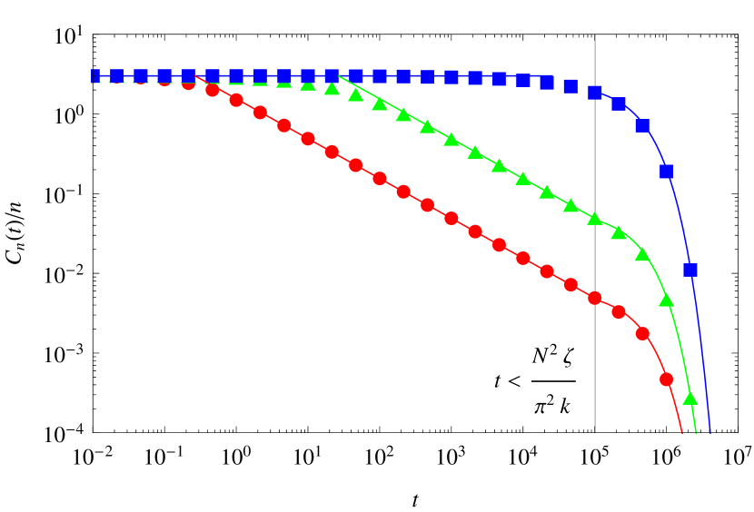
Figure 3: The scaled correlation function $C_{n}(t)/n$ as defined in Eqs. (21-22) in a double-logarithmic plot as a function of time. The correlation functions for several monomers in a symmetric star polymer as given by Eq. (II.3) were exactly evaluated with $f=12$ arms of length $N=10^{3}$ and other parameters put to $1$. The red disks, green triangles, and blue squares correspond to $n=1,10$, and $N$ for $C_{n}(t)$ respectively. Approximations for the correlation function in the short time scale $t<\zeta(n+1)^{2}/(4\pi^{2}k)$, intermediate time scale $\zeta n^{2}(f-1)^{2}/(k\pi f^{2})<t<N^{2}\zeta/(\pi^{2}k)$, and the very long time scale $t>N^{2}\zeta/(\pi^{2}k)$ as in Eq. (25) correspond solid lines. The approximation for intermediate times is only very accurate for small $n$, but for larger $n$ this time domain becomes smaller or even non-existent as is the case for $n$ equals $N$ as can be seen in the figure.

The correlation function $C_{n}(t)\equiv\langle{\bf r}_{i,n}(t)\cdot{\bf r}_{i,n}(0)\rangle$ is then given by

$$C_{n}(t)= 16\sum_{p=1}^{N}\sin^{2}\left[\frac{\pi(n+1)p/2}{N+1}\right]\sin^{2}\left[\frac{\pi np/2}{N+1}\right]X_{pp}(t)$$

$$+\frac{16}{f^{2}}\sum_{j,k,p=1}^{f,f,N}\cos^{2}\left[\frac{\pi(N-n+1/2)(p-1/2)}{N+1/2}\right]Y_{pp}^{(i,k)(i,j)}(t),$$ (22)

where the cosines were reduced to sines for notational convenience. Having filled in the mode dynamics functions explicitly yields

$$C_{n}(t)= \frac{24k_{B}T}{\zeta f(N+1)}\sum_{p=1}^{N}\sin^{2}\left[\frac{\pi(n+1)p/2}{N+1}\right]\sin^{2}\left[\frac{\pi np/2}{N+1}\right]\frac{1}{\alpha_{{\bf X}_{p}}}\exp\left[-\alpha_{{\bf X}_{p}}t\right]$$

$$+\frac{12(f-1)k_{B}T}{\zeta f(2N+1)}\sum_{p=1}^{N}\cos^{2}\left[\frac{\pi(N-n+1/2)(p-1/2)}{N+1/2}\right]\frac{1}{\alpha_{{\bf Y}_{p}}}\exp\left[-\alpha_{{\bf Y}_{p}}t\right],$$ (23)

where $\alpha_{{\bf X}_{p}}$ and $\alpha_{{\bf Y}_{p}}$ are defined in Eqs. (40-41). At very large and very small times the exact correlation functions for the modes in Eq. (43) can be used. At very small times the exponential can be omitted and the resulting equations solved using Eqs. (46b,46d). Adding the two terms then results in $C_{n}(t)=3nk_{B}T/k$. To determine the region for which this approximation is valid we notice that the exponent is roughly $1$ for $p^{2}<\zeta N^{2}/(\pi^{2}kt)$. The term in the summation will go to $0$ for $p=2(N+1)/(n+1)$ and so the largest contribution to the summation is for all the terms before this happens. Solving this for $t$ where the large polymer limit is taken gives $t<\zeta(n+1)^{2}/(4\pi^{2}k)$ for which the approximation is valid. For very large time values $t>(N^{2}\zeta)(\pi^{2}k)$ only the lowest mode will give contribution. Since $f=1,2$ are two cases of linear chains we focus on $f\geq 3$ for which the second term in Eq. (II.3) will dominate. Taking the long polymer limit the sine can be expanded and the cosine reduced for notational convenience. For very large times the correlation function can thus be approximated by $C_{n}(t)=12k_{B}TN/(\pi^{2}k)\left(1-\cos\left[\pi n/N\right]\right)\exp\left[-\pi^{2}kt/(4\zeta N^{2})\right]$. For intermediate time values the second term can be approximated by a Gaussian integral in the long polymer limit by expanding the cosine for small $n$.

$$C_{n}(t)= \frac{6(f-1)n^{2}k_{B}T}{kf}\int_{0}^{\infty}dx\exp\left[-\frac{\pi^{2}kt}{\zeta}x^{2}\right]=\frac{3(f-1)n^{2}k_{B}T}{kf\sqrt{\pi}}\left(\frac{kt}{\zeta}\right)^{-1/2}.$$ (24)

For $t>\zeta n^{2}(f-1)^{2}/(\pi kf^{2})$ the intermediate time approximation will be smaller and thus more accurate than the approximation for small times. Putting this together gives for $f\geq 3$

$$C_{n}(t)=\left\{\begin{array}[]{ll}\displaystyle{\frac{3nk_{B}T}{k},\quad\quad\quad\quad\quad\quad\quad\quad\quad\quad\quad\quad\quad\quad\quad\,\,\mbox{for}\,t<\frac{\zeta(n+1)^{2}}{4\pi^{2}k}}\\ \displaystyle{\frac{3(f-1)n^{2}k_{B}T}{kf\sqrt{\pi}}\left(\frac{kt}{\zeta}\right)^{-1/2},\,\quad\quad\quad\quad\quad\quad\quad\mbox{for}\,\frac{\zeta n^{2}(f-1)^{2}}{k\pi f^{2}}<t<\frac{N^{2}\zeta}{\pi^{2}k}}\\ \displaystyle{\frac{12k_{B}TN}{\pi^{2}k}\left(1-\cos\left[\frac{\pi n}{N}\right]\right)\exp\left[-\frac{\pi^{2}k}{4\zeta N^{2}}t\right],\,\,\,\mbox{for}\,t>\frac{N^{2}\zeta}{\pi^{2}k}}\end{array}\right..$$ (25)

A graphical representation of the correlation function for a spatial vector between some monomer and the central monomer in a symmetric starpolymer with $f=12$ and $N=10^{5}$ is shown in Fig. 3.

III Dynamical eigenmodes of tadpole polymers

A tadpole polymer can be seen as a star polymer where two of the three arms have the ends connected. Here we extend our calculations of the previous section and write down the exact solution for the eigenmodes for the specific case where the tadpole is built from a symmetric star polymer with arms of length $N$ and a central bead with hydrodynamic radius three times as large as that of all the other beads. The Rouse modes are then a variation of the modes for a ring polymer combined with those for a star polymer. The first set of $N+1$ modes are like the ${\bf X}$ modes for the star polymer where all the arms behave the same. The second set of $N$ modes are very similar to the ${\bf Y}$ modes of the star polymer where the ring takes on the role of an arm and the tail of the tadpole the role of another arm. The third set ${\bf Z}$ of $N$ modes are Rouse modes for a ring polymer but specifically such that it is antisymmetric around the central bead. In Fig. 4 these three different modes are depicted for $p=1$.

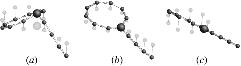
Figure 4: Three graphical representations of a tadpole polymer to visualize the Rouse modes. Depicted is a tadpole polymer, which can be seen as a symmetric star polymer with three arms consisting of four beads each where two arms are connected at the ends, with a central monomer which has a friction coefficient three times that of beads in the arms. The transparent configurations are polymers in the origin stretched in the $xy$-plane for visual convenience with no Rouse mode excited in the $z$-direction. The opague configurations are like the transparent ones but with a pure ${\bf X}_{1}$ mode (a), ${\bf Y}_{1}$ mode (b), and ${\bf Z}_{1}$ mode (c) in the z-direction.

We label the tadpole polymer like a three-armed symmetric star polymer where arm one and two have the ends connected. The Rouse modes are then given by

$${\bf X}_{p}(t) = \frac{1}{N+1}\left\{\cos\left[\frac{\pi p/2}{N+1}\right]{\bf R}_{0}(t)+\frac{1}{3}\sum_{a,n=1}^{3,N}\cos\left[\frac{\pi(n+1/2)p}{N+1}\right]{\bf R}_{a,n}(t)\right\},$$ (26a)

$${\bf Y}_{q}(t) = \frac{1}{4N+2}\!\sum_{n=1}^{N}\!\cos\!\left[\frac{\pi(N-n+1/2)(q-1/2)}{N+1/2}\right]\!\left[{\bf R}_{1,n}(t)+{\bf R}_{2,n}(t)-2{\bf R}_{3,n}(t)\right]\!,$$ (26b)

$${\bf Z}_{q}(t) = \frac{1}{2N+1}\sum_{n=1}^{N}\sin\left[\frac{\pi(N-n+1/2)q}{N+1/2}\right]\left({\bf R}_{1,n}(t)-{\bf R}_{2,n}(t)\right),$$ (26c)

with $p=0\dots N$ and $q=1\dots N$. The validity of these Rouse modes as the dynamical eigenmodes can be proved like for the star polymer in Appendix A. Let us define

$${\bf\widetilde{X}}_{n}(t) = {\bf X}_{0}(t)+2\sum_{p=1}^{N}\cos\left[\frac{\pi(n+1/2)p}{N+1}\right]{\bf X}_{p}(t),$$ (27a)

$${\bf\widetilde{Y}}_{n}(t) = \frac{4}{3}\sum_{p=1}^{N}\cos\left[\frac{\pi(N-n+1/2)(p-1/2)}{N+1/2}\right]{\bf Y}_{p}(t),$$ (27b)

$${\bf\widetilde{Z}}_{n}(t) = 2\sum_{p=1}^{N}\sin\left[\frac{\pi(N-n+1/2)p}{N+1/2}\right]{\bf Z}_{p}(t),$$ (27c)

so that the bead locations are given by

$${\bf R}_{0}(t) = {\bf\widetilde{X}}_{0}(t)$$ (28a)

$${\bf R}_{1,n}(t) = {\bf\widetilde{X}}_{n}(t)+{\bf\widetilde{Y}}_{n}(t)+{\bf\widetilde{Z}}_{n}(t),$$ (28b)

$${\bf R}_{2,n}(t) = {\bf\widetilde{X}}_{n}(t)+{\bf\widetilde{Y}}_{n}(t)-{\bf\widetilde{Z}}_{n}(t),$$ (28c)

$${\bf R}_{3,n}(t) = {\bf\widetilde{X}}_{n}(t)-2{\bf\widetilde{Y}}_{n}(t).$$ (28d)

The dynamics for these modes are very similar as for the modes of the star polymer. The non-vanishing correlation functions for the modes of the tadpole are then given by

$$\langle[{\bf X}_{0}(t)-{\bf X}_{0}(0)]^{2}\rangle=\frac{2k_{B}T}{\zeta(N+1)}t$$ (29a)

$$\langle{\bf X}_{p}(t)\cdot{\bf X}_{q}(0)\rangle=\frac{k_{B}T}{\zeta(N+1)}\frac{1}{2\alpha_{{\bf X}_{p}}}\exp\left[-\alpha_{{\bf X}_{p}}t\right]\delta_{pq}$$ (29b)

$$\langle{\bf Y}_{p}(t)\cdot{\bf Y}_{q}(0)\rangle=\frac{9k_{B}T}{4\zeta(2N+1)}\frac{1}{2\alpha_{{\bf Y}_{p}}}\exp\left[-\alpha_{{\bf Y}_{p}}t\right]\delta_{pq}$$ (29c)

$$\langle{\bf Z}_{p}(t)\cdot{\bf Z}_{q}(0)\rangle=\frac{3k_{B}T}{\zeta(2N+1)}\frac{1}{2\alpha_{{\bf Z}_{p}}}\exp\left[-\alpha_{{\bf Z}_{p}}t\right]\delta_{pq},$$ (29d)

for $p,q=1,\dots N$ and

$$\alpha_{{\bf X}_{p}}=4\frac{k}{\zeta}\sin^{2}\left[\frac{\pi p}{2N+2}\right],\alpha_{{\bf Y}_{p}}=4\frac{k}{\zeta}\sin^{2}\left[\frac{\pi(p-1/2)}{2N+1}\right],\alpha_{{\bf Z}_{p}}=4\frac{k}{\zeta}\sin^{2}\left[\frac{\pi p}{2N+1}\right].$$ (30)

III.1 Radius of gyration

When the ends of two arms of a three armed symmetric star polymer are connected the mobility reduces and the radius of gyration will become smaller. Following the same steps as for the star polymer the radius of gyration is defined in the same way for the case when the central bead is three times as heavy as any other bead, and by plugging in the inverses it can be rewritten in terms of summations over the correlation functions of the modes at time zero. The radius of gyration squared for a long tadpole becomes:

$$R_{g}^{2} =\frac{k_{B}TN}{k}\frac{5}{6},$$ (31)

which is $5/7$th of the radius of gyration of the same polymer but with the ends not connected.

III.2 Mean square displacement of a monomer

Since the tadpole can be seen as a three armed star polymer with ends of two of the arms connected, the mean square displacement of the monomers in the third arm and that of the central monomer will not feel the effect of the connection of the two remaining arms. And so for the central monomer and the monomers in the tail of the tadpole the expressions will be exactly the same as in Eqs. (13,17) respectively. A monomer in the closed circle of the tadpole should behave in the same way as some monomer roughly in the middle of the tail:

$$\Delta{\bf R}_{0}(t)\equiv{\bf R}_{0}(t)-{\bf R}_{0}(0)\quad,\quad\Delta{\bf R}_{i,n}(t)\equiv{\bf R}_{i,n}(t)-{\bf R}_{i,n}(0).$$ (32)

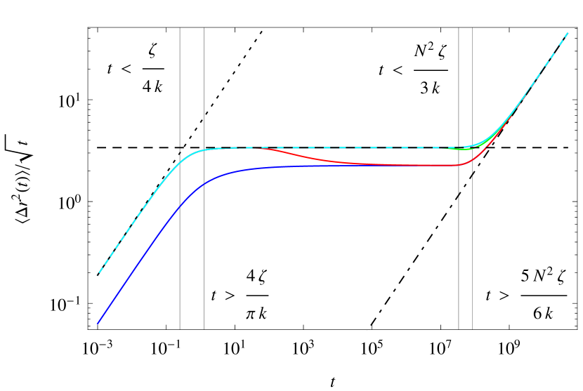
Figure 5: The scaled mean square displacement $\langle\Delta{\bf R}^{2}(t)\rangle/\sqrt{t}$ as a function of time. The mean square displacement of several beads in a tadpole made by a symmetric star polymer with ends of arm $1$ and $2$ connected as defined by Eq. (32) were exactly evaluated with $N=10^{4}$ and other parameters put to $1$. The solid blue line corresponds to the mean square displacement of the central bead whereas the red, green, magenta, and cyan solid lines correspond to $i=1$ and $n=10^{-3}N,N/2,9N/10$, and $N$ in Eq. (32) respectively. Unlike for the unconnected arms in the star polymer here there is no real difference between a monomer at the middle or end of the connected arm. A bead positioned somewhere along the arm will at first behave as if it were in the middle of the arm. If it is close enough to the heavy central bead the movement will be restricted and the mean square displacement will mimic that of the central bead. The short time scale $t<\zeta/(4k)$ and the very long time scale $t\gg 5N^{2}\zeta/(6k)$ for which $\langle\Delta{\bf R}^{2}(t)\rangle\sim t$ corresponding to the dotted and dot-dashed lines are separated by a time during which $\langle\Delta{\bf R}^{2}(t)\rangle\sim\sqrt{t}$ corresponding to the dashed line as in agreement with Eqs. (33).

The mean square displacement for monomers in a tadpole can be described by

$$\langle\Delta{\bf R}_{0}^{2}(t)\rangle=\left\{\begin{array}[]{ll}\displaystyle{\frac{2k_{B}T}{\zeta}t,\quad\quad\quad\quad\mbox{for}\,t<\frac{\zeta}{4k}}\\ \displaystyle{4k_{B}T\sqrt{\frac{t}{\pi k\zeta}},\quad\,\,\,\,\mbox{for}\,\frac{4\zeta}{\pi k}<t<\frac{N^{2}\zeta}{3k}}\\ \displaystyle{\frac{2k_{B}T}{\zeta N}t,\quad\quad\quad\quad\mbox{for}\,t>\frac{N^{2}\zeta}{3k}}\end{array}\right.,$$ (33a)

$$\langle\Delta{\bf R}_{3,N}^{2}(t)\rangle=\left\{\begin{array}[]{ll}\displaystyle{\frac{6k_{B}T}{\zeta}t,\quad\quad\quad\quad\mbox{for}\,t<\frac{\zeta}{4k}}\\ \displaystyle{12k_{B}T\sqrt{\frac{t}{\pi k\zeta}},\quad\,\,\,\,\mbox{for}\,\frac{4\zeta}{\pi k}<t<\frac{N^{2}\zeta}{3k}}\\ \displaystyle{\frac{2k_{B}T}{\zeta N}t,\quad\quad\quad\quad\mbox{for}\,t>\frac{7N^{2}\zeta}{3k}}\end{array}\right.,$$ (33b)

$$\langle\Delta{\bf R}_{1,N}^{2}(t)\rangle=\langle\Delta{\bf R}_{3,N/2}^{2}(t)\rangle=\left\{\begin{array}[]{ll}\displaystyle{\frac{6k_{B}T}{\zeta}t,\quad\quad\quad\quad\mbox{for}\,t<\frac{\zeta}{4k}}\\ \displaystyle{6k_{B}T\sqrt{\frac{t}{\pi k\zeta}},\quad\,\,\,\,\mbox{for}\,\frac{4\zeta}{\pi k}<t<\frac{N^{2}\zeta}{3k}}\\ \displaystyle{\frac{2k_{B}T}{\zeta N}t,\quad\quad\quad\quad\mbox{for}\,t>\frac{5N^{2}\zeta}{6k}}\end{array}\right..$$ (33c)

Note that the domains of validity for the different behavior have changed in comparison to the star polymer. The exact sums for the monomers in a tadpole have a slightly different maximum as can be calculated using Eq. (46).

IV Discussion

For bead-spring models of polymers with the topology of a symmetric star with $f$ arms, where the hydrodynamic radius of the central bead is $f$ times as heavy as any other bead, we derived the exact expressions for the dynamical eigenmodes. We demonstrated the usefulness of this exercise by exact calculations of various quantities that yield prefactors as well as give insights into the scaling behavior at different time regimes for these quantities. The radius of gyration was shown to be given by $R_{g}^{2}=k_{B}TN(3f-2)/(2kf)$; the mean square displacement of the central bead and of various other individual beads was shown to scale as $\sim t$ at very short as well as at very long times, with an intermediate regime in which it scales as $\sim\sqrt{t}$; and the correlation function of an orientational vector was shown to stay invariant at very short times, decay exponentially at very long times, and decay as $\sim 1/\sqrt{t}$ in the intermediate regime. Similar results were also derived for tadpoles, which are $f=3$ star polymers in which two arms are connected.

Our exact results are limited to the very specific case of $f$-arm star polymers and tadpoles in which the hydrodynamic radius of the central bead is exactly $f$ times bigger than the other beads. The Rouse modes can still be constructed for other cases, since the Rouse equations are linear in the bead positions; indeed, this has already been achieved numericallystarthesis . We do not rule out analytical forms of the Rouse modes for these cases, although we can expect that these analytical forms may not look aesthetically pleasant. Even if the hydrodynamic radius of the central bead is not exactly $f$ times bigger than the other beads, we do not forsee differences in the behavior of the mean-square displacements in the scaling limit, namely the three regimes mentioned above, albeit with different prefactors. The same should hold for modest modifications of the interatomic bonds: no qualitatively different behavior is expected, but prefactors will be affected. As for the dynamical eigenmodes of star and tadpole polymers, qualitative differences will however arise due to significant hydrodynamic interactions between the beads, excluded-volume effects, or if the solution is no longer dilute.

Apart from these direct results, the usefulness of our exercise lies perhaps even more in providing a proper language in which to characterize the dynamics of star and tadpole polymers; very similar to the ubiquitous use of Rouse mode amplitudes for linear polymers.

In future work, we will use the mathematical expressions for the Rouse modes derived here, to characterize the dynamics of star polymers in simulations of self-avoiding stars, in dilute circumstances, as well as in various dense environments (such as a melt of linear polymers, or a homodisperse melt of star polymers).

Appendix A Determination of the Rouse modes of a star polymer

Several steps are needed to derive the dynamics of the modes (7) from the equations of motion for a symmetric star polymer. It is useful to note that the modes are complete, which allows us to express the positions of the beads from the mode amplitudes, given by

$${\bf R}_{0}= {\bf X}_{0}+2\sum_{p=1}^{N}\cos\left[\frac{\pi p/2}{N+1}\right]{\bf X}_{p}$$ (34a)

$${\bf R}_{i,n}= {\bf X}_{0}+2\sum_{p=1}^{N}\cos\left[\frac{\pi(n+1/2)p}{N+1}\right]{\bf X}_{p}+\frac{4}{f}\sum_{j,p=1}^{f,N}\cos\left[\frac{\pi(N-n+1/2)(p-1/2)}{N+1/2}\right]{\bf Y}_{p}^{(i,j)}.$$ (34b)

The correctness of these equations can be checked using the orthogonality relations (44).

The dynamical equations of motion for the star polymer combined with the potential energy then result in the following equation of motion for the beads:

$$\frac{d{\bf R}_{0\,\,\,\,}}{dt} =-\frac{k}{\zeta}\left({\bf R}_{0}-\frac{1}{f}\sum_{i=1}^{f}{\bf R}_{i,1}\right)+{\bf g}_{0}$$ (35a)

$$\frac{d{\bf R}_{i,1}}{dt} =-\frac{k}{\zeta}\left(2{\bf R}_{i,1}-{\bf R}_{0}-{\bf R}_{i,2}\right)+{\bf g}_{i,1}$$ (35b)

$$\frac{d{\bf R}_{i,n}}{dt} =-\frac{k}{\zeta}\left(2{\bf R}_{i,n}-{\bf R}_{i,n-1}-{\bf R}_{i,n+1}\right)+{\bf g}_{i,n}.$$ (35c)

Note that $i=1\dots f$ and Eq. (35c) is valid for all $n=2\dots N$ where Eq. (34b) is needed to show that ${\bf R}_{i,N+1}={\bf R}_{i,N}$. For convenience we define

$${\bf R}_{n}=\frac{1}{f}\sum_{i=1}^{f}{\bf R}_{i,n}={\bf X}_{0}+2\sum_{p=1}^{N}\cos\left[\frac{\pi(n+1/2)p}{N+1}\right]{\bf X}_{p},$$ (36)

for $n=0\dots N$ which coincides with the inverse of ${\bf R}_{0}$ as given in Eq. (34a). Taking the time derivative on both sides of Eq. (6a), plugging in the equations of motion for the beads from Eq. (35), and using the definition above for which ${\bf R}_{-1}={\bf R}_{0}$ and ${\bf R}_{N+1}={\bf R}_{N}$ results in

$$\frac{d{\bf X}_{p}}{dt}=-\frac{1}{N+1}\frac{k}{\zeta}\sum_{n=0}^{N}\cos\left[\frac{\pi(n+1/2)p}{N+1}\right]\left(2{\bf R}_{n}-{\bf R}_{n-1}-{\bf R}_{n+1}\right)+{\bf G}_{p}\,\,,$$ (37)

where ${\bf G}_{p}$ is the transform of the thermal forces which will be calculated later. By using (36), the trigonometric identities, namely the angle sum and difference identities and the power-reduction formula, and finally the orthogonality relation the set of differential equations becomes

$$\frac{d{\bf X}_{p}}{dt}=\left\{\begin{array}[]{ll}-\alpha_{{\bf X}_{p}}{\bf X}_{p}+{\bf G}_{p},\quad p=1\dots N\\ {\bf G}_{0}\qquad\qquad\quad,\quad p=0\end{array}\right.,\quad\alpha_{{\bf X}_{p}}=4\frac{k}{\zeta}\sin^{2}\left[\frac{\pi p}{2N+2}\right].$$ (40)

The set of differential equations for the ${\bf Y}^{(i,j)}_{p}$ modes can be written down in a similar manner. We define ${\bf R}_{n}^{(i,j)}\equiv{\bf R}_{i,n}-{\bf R}_{j,n}$ and follow similar steps as for the ${\bf X}_{p}$ modes so that

$$\frac{d{\bf Y}_{p}^{(i,j)}}{dt}=-\alpha_{{\bf Y}_{p}}{\bf Y}_{p}+{\bf G}_{p}^{(i,j)},\quad p=1\dots N,\quad\alpha_{{\bf Y}_{p}}\equiv 4\frac{k}{\zeta}\sin^{2}\left[\frac{\pi(p-1/2)}{2N+1}\right]$$ (41)

for some transform of the thermal forces ${\bf G}_{p}^{(i,j)}$.

With the above transformations, the set of differential equations for the beads have been transformed to a set of disconnected linear differential equations.

To find the relation for the modes as in Eq. (7) we must first determine the transform of the thermal forces ${\bf G}_{p}$ and ${\bf G}_{p}^{(i,j)}$. The transforms are equal to that of the modes in Eq. (6) but by replacing the position of the beads by their thermal force. Use that the thermal forces are uncorrelated in time and between beads as in Eq. (3) and recall that the central bead has a friction coefficient $f$ times as large as that of the other beads. The only nonvanishing functions with $p=1\dots N$ are

$$\left\langle{\bf G}_{0}(t)\cdot{\bf G}_{0}(t^{\prime})\right\rangle =\frac{6k_{B}T}{\zeta f(N+1)}\delta(t-t^{\prime})$$ (42a)

$$\left\langle{\bf G}_{p}(t)\cdot{\bf G}_{q}(t^{\prime})\right\rangle =\frac{3k_{B}T}{\zeta f(N+1)}\delta_{pq}\delta(t-t^{\prime})$$ (42b)

$$\left\langle{\bf G}_{p}^{(i,j)}(t)\cdot{\bf G}_{q}^{(k,l)}(t^{\prime})\right\rangle =\frac{3k_{B}T}{\zeta(2N+1)}\delta_{pq}\delta(t-t^{\prime})\frac{\delta_{(i,j),(k,l)}}{2}.$$ (42c)

With these, the set of differential equations can be solved exactly resulting in the following relations between modes:

$$\langle[{\bf X}_{0}(t)-{\bf X}_{0}(0)]^{2}\rangle=\frac{6k_{B}T}{\zeta f(N+1)}t$$ (43a)

$$\langle{\bf X}_{p}(t)\cdot{\bf X}_{q}(0)\rangle=\frac{3k_{B}T}{\zeta f(N+1)}\frac{1}{2\alpha_{{\bf X}_{p}}}\exp\left[-\alpha_{{\bf X}_{p}}t\right]\delta_{pq}$$ (43b)

$$\langle{\bf Y}_{p}^{(i,j)}(t)\cdot{\bf Y}_{q}^{(k,l)}(0)\rangle=\frac{3k_{B}T}{\zeta(2N+1)}\frac{\delta_{(i,j)(k,l)}}{2}\frac{1}{2\alpha_{{\bf Y}_{p}}}\exp\left[-\alpha_{{\bf Y}_{p}}t\right]\delta_{pq},$$ (43c)

where all other correlations between modes are strictly zero. By taking the long-polymer limit the sines can be expanded up to second order and the results are in Eq. (7).

Appendix B Useful mathematical relations

The following relations are useful for calculating the Rouse modes:

$$\frac{2}{N+1}\sum_{n=0}^{N}\cos\left[\frac{\pi(n+1/2)p}{N+1}\right]\cos\left[\frac{\pi(n+1/2)q}{N+1}\right]=\delta_{pq}$$ (44a)

$$\frac{4}{2N+1}\sum_{n=1}^{N}C_{p}C_{q}=\delta_{pq}\quad,\quad C_{p}=\cos\left[\frac{\pi(N-n+1/2)(p-1/2)}{N+1/2}\right],$$ (44b)

$$\frac{4}{2N+1}\sum_{n=1}^{N}C_{p}C_{q}=\delta_{pq}\quad,\quad C_{p}=\sin\left[\frac{\pi(N-n+1/2)p}{N+1/2}\right],$$ (44c)

for $p,q=1\dots N$ and where the left hand side of Eq. (44a) equals $2\delta_{p0}$ for $p=0\dots N$.

$$\sum_{p=1}^{N}\cos^{2}\left[\frac{\pi(n+1/2)p}{N+1}\right]=\frac{N}{2},\quad n=0\dots N$$ (45a)

$$\sum_{p=1}^{N}\cos^{2}\left[\frac{\pi(N-n+1/2)(p-1/2)}{N+1/2}\right]=\frac{2N+1}{4},\quad n=1\dots N$$ (45b)

$$\sum_{p=1}^{N}\sin^{2}\left[\frac{\pi(N-n+1/2)p}{N+1/2}\right]=\frac{2N+1}{4},\quad n=1\dots N$$ (45c)

$$\sum_{p=1}^{N}\cos^{2}\left[\frac{\pi(n+1/2)p}{N+1}\right]\sin^{-2}\left[\frac{\pi p}{2N+2}\right]=\frac{N}{3}(2N+1)-2Nn+2n^{2}$$ (46a)

$$\sum_{p=1}^{N}\cos^{2}\left[\frac{\pi(N-n+1/2)(p-1/2)}{N+1/2}\right]\sin^{-2}\left[\frac{\pi(p-1/2)}{2N+1}\right]=(2N+1)n$$ (46b)

$$\sum_{p=1}^{N}\sin^{2}\left[\frac{\pi(N-n+1/2)p}{N+1/2}\right]\sin^{-2}\left[\frac{\pi p}{2N+1}\right]=(2N+1-2n)n$$ (46c)

$$\sum_{p=1}^{N}\sin^{2}\left[\frac{\pi(n+1)p/2}{N+1}\right]\sin^{2}\left[\frac{\pi np/2}{N+1}\right]\sin^{-2}\left[\frac{\pi p/2}{N+1}\right]=\frac{n}{2}(N+1)$$ (46d)

$$\sum_{p=1}^{\infty}\frac{1}{p^{2}}=\frac{\pi^{2}}{6}$$ (47a)

$$\sum_{p=1}^{\infty}\frac{1}{(p-1/2)^{2}}=\frac{\pi^{2}}{2}\qquad$$ (47b)

References

- (1) P. E. Rouse Jr., J. Chem. Phys. 21, 1272 (1953)
- (2) M. Doi, Introduction to Polymer Physics, Oxford University Press (Reprinted, 2001).
- (3) M. Doi and S. F. Edwards, The theory of polymer dynamics, Clarendon Press, Oxford (Reprinted, 2001).
- (4) D. Panja, J. Stat. Mech. L02001 (2010).
- (5) D. Panja, J. Stat. Mech. P06011 (2010).
- (6) D. Panja and G.T. Barkema, J. Chem. Phys. 131, 154903 (2009).
- (7) G.T. Barkema, D. Panja and J.M.J. van Leeuwen, J. Chem. Phys. 134, 154901 (2011).
- (8) A. Ghosh, “Relaxation dynamics of branched polymers”, Ph.D. thesis (Material Science and Engineering, Pennsylvania State University, 2007).
- (9) H. Gao and K. Matyjaszewski, Prog. Polym. Sci. 34, 317 (2009).