Minimax properties of Fréchet means of discretely sampled curves

Abstract

We study the problem of estimating a mean pattern from a set of similar curves in the setting where the variability in the data is due to random geometric deformations and additive noise. We propose an estimator based on the notion of Fréchet mean that is a generalization of the standard notion of averaging to non-Euclidean spaces. We derive a minimax rate for this estimation problem, and we show that our estimator achieves this optimal rate under the asymptotics where both the number of curves and the number of sampling points go to infinity.

and t1Supported by the French Agence Nationale de la Recherche (ANR) under reference ANR-JCJC-SIMI1 DEMOS.

1 Introduction

1.1 Fréchet means

The Fréchet mean fre is an extension of the usual Euclidean mean to nonlinear spaces endowed with non-Euclidean metrics. If $\mathbf{Y}_{1},\ldots,\mathbf{Y}_{J}$ denote i.i.d. random variables with values in a metric space $\mathcal{M}$ with metric $d_{\mathcal{M}}$, then the empirical Fréchet mean $\overline{\mathbf{Y}}_{\mathcal{M}}$ of the sample $\mathbf{Y}_{1},\ldots,\mathbf{Y}_{J}$ is defined as a minimizer (not necessarily unique) of

$$\overline{\mathbf{Y}}_{\mathcal{M}}\in\mathop{\operatorname{argmin}}_{y\in\mathcal{M}}\frac{1}{J}\sum_{j=1}^{J}d_{\mathcal{M}}^{2}(y,\mathbf{Y}_{j}).$$

For random variables belonging to a nonlinear manifold, a well-known example is the computation of the mean of a set of planar shapes in Kendall’s shape space kendall that leads to the Procrustean means studied in MR1108330 . A detailed study of some properties of the Fréchet mean in finite dimensional Riemannian manifolds (such as consistency and uniqueness) has been performed in Afsari , batach1 , batach2 , MR2816349 . However, there is not so much work on the properties of the Fréchet mean in infinite dimensional and non-Euclidean spaces of curves or images. In this paper, we are concerned with the nonparametric estimation of a mean pattern (belonging to a nonlinear space) from a set of similar curves in the setting where the variability in the data is due to random geometric deformations and additive noise.

More precisely, let us consider noisy realizations of $J$ curves $f_{1},\ldots,f_{J}\dvtx\break[0,1]\to\mathbb{R}$ sampled at $n$ equispaced points $t_{\ell}=\frac{\ell}{n},\ell=1,\ldots,n$,

$$Y_{\ell,j}=f_{j}(t_{\ell})+\varepsilon_{\ell,j},\qquad\ell=1,\ldots,n\mbox{ and }j=1,\ldots,J,$$ (1)

where the $\varepsilon_{\ell,j}$’s are independent and identically distributed (i.i.d.) Gaussian variables with zero expectation and known variance $\sigma^{2}>0$. In many applications, the observed curves have a similar structure that may lead to the assumption that the $f_{j}$’s are random elements varying around the same mean pattern $f\dvtx[0,1]\to\mathbb{R}$ (also called reference template). However, due to additive noise and geometric variability in the data, this mean pattern is typically unknown and has to be estimated. In this setting, a widely used approach is Grenander’s pattern theory Gre , gremil , MR2176922 , TYShape that models geometric variability by the action of a Lie group on an infinite dimensional space of curves (or images).

When the curves $f_{j}$ in (1) exhibit a large source of geometric variation in time, this may significantly complicates the construction of a consistent estimator of a mean pattern. In what follows, we consider the simple model of randomly shifted curves that is commonly used in many applied areas such as neurosciences MR2816476 or biology MR1841413 . In such a framework, we have

$$f_{j}(t)=f\bigl{(}t-\theta_{j}^{\ast}\bigr{)}\qquad\mbox{for all }t\in[0,1]\mbox{ and }j=1,\ldots,J,$$ (2)

where $f\dvtx[0,1]\to\mathbb{R}$ is an unknown curve that can be extended outside $[0,1]$ by $1$-periodicity. In a similar way, we could consider a function $f$ defined on the circle $\mathbb{R}/\mathbb{Z}$. The shifts $\theta_{j}^{\ast}$’s are supposed to be i.i.d. real random variables (independent of the $\varepsilon_{\ell,j}$’s) that are sampled from an unknown distribution $\mathbb{P}_{\ast}$ on $\mathbb{R}$. In model (2), the shifts $\theta_{j}^{\ast}$ represent a source of geometric variability in time.

In functional data analysis, the problem of estimating a mean pattern from a set of curves that differ by a time transformation is usually referred to as the curve registration problem; see, for example, ramsil . Registering functional data has received a lot of attention in the literature over the two last decades; see, for example, big , kneipgas , ramsil , tangmull , wanggas and references therein. Nevertheless, in these papers, constructing consistent estimators of the mean pattern $f$ as the number $J$ of curves tends to infinity is generally not considered. Self-modeling regression methods proposed in kg are semiparametric models for curve registration that are similar to the shifted curves model, where each observed curve is a parametric transformation of an unknown mean pattern. Constructing a consistent estimator of the mean pattern in such models has been investigated in kg in an asymptotic framework where both the number $J$ of curves and the number $n$ of design points grow toward infinity. However, deriving optimal estimators in the minimax sense has not been considered in kg . Moreover, a novel contribution of this paper is to make a connection between the curve registration problem and the notion of Fréchet mean in non-Euclidean spaces which has not been investigated so far.

1.2 Model and objectives

The main goal of this paper is to construct nonparametric estimators of the mean pattern $f$ from the data

$$Y_{\ell,j}=f\bigl{(}t_{\ell}-\theta_{j}^{\ast}\bigr{)}+\varepsilon_{\ell,j},\qquad\ell=1,\ldots,n\mbox{ and }j=1,\ldots,J,$$ (3)

in the setting where both the number $J$ of curves and the number $n$ of design points are allowed to vary and to tend toward infinity.

In the sequel to this paper, it will be assumed that the random shifts are sampled from an unknown density $g$ with respect to the Lebesgue measure $d\theta$ [namely $d\mathbb{P}_{\ast}(\theta)=g(\theta)\,d\theta$]. Note that since $f$ is assumed to be $1$-periodic, one may restrict to the case where the density $g$ has a compact support included in the interval $[-\frac{1}{2},\frac{1}{2}]$. Under assumption (2), the (standard) Euclidean mean $\bar{Y}_{\ell}=\frac{1}{J}\sum_{j=1}^{J}Y_{\ell,j}$ of the data is generally not a consistent estimator of the mean pattern $f$ at $t=t_{\ell}$. Indeed, the law of large numbers implies that

$$\lim_{J\to\infty}\bar{Y}^{\ell}=\lim_{J\to\infty}\frac{1}{J}\sum_{j=1}^{J}f\bigl{(}t_{\ell}-\theta_{j}^{\ast}\bigr{)}=\int_{\mathbb{R}}f(t_{\ell}-\theta)g(\theta)\,d\theta\qquad\mbox{a.s.}$$

Thus, under mild assumptions on $f$ and $g$, we have

$$\lim_{J\to\infty}\bar{Y}^{\ell}=f\star g(t_{\ell})\neq f(t_{\ell})\qquad\mbox{a.s.},$$

where $f\star g$ is the convolution product between $f$ and $g$.

To build a consistent estimator of $f$ in model (3), we propose to use a notion of empirical Fréchet mean in an infinite dimensional space. Recently, some properties of Fréchet means in randomly shifted curves models have been investigated in MR2676894 and BC11 . However, studying the rate of convergence and the minimax properties of such estimators in the double asymptotic setting $\min(n,J)\to+\infty$ has not been considered so far.

Note that model (3) is clearly not identifiable, as for any $\tilde{\theta}\in[-\frac{1}{2},\frac{1}{2}]$, one may replace $f(\cdot)$ by $\tilde{f}(\cdot)=f(\cdot-\tilde{\theta})$ and $\theta_{j}^{\ast}$ by $\tilde{\theta}_{j}=\theta_{j}^{\ast}-\tilde{\theta}$ without changing model (3). Therefore, estimation of $f$ is only feasible up to a time shift. Thus, we propose to consider the problem of estimating its equivalence class $[f]$ (or orbit) under the action of shifts. More precisely, let $L^{2}_{\mathrm{per}}([0,1])$ be the space of squared integrable functions on $[0,1]$ that can be extended outside $[0,1]$ by 1-periodicity. Let $\mathbb{S}_{1}$ be the one-dimensional torus. We recall that any element $\tau=\tau(\theta)\in\mathbb{S}_{1}$ can be identified with an element $\theta$ in the interval $[-\frac{1}{2},\frac{1}{2}]$. For $f\in L^{2}_{\mathrm{per}}([0,1])$, we define its equivalence class by the action of a time shift as

$$[f]:=\bigl{\{}f^{\tau},\tau\in\mathbb{S}_{1}\bigr{\}},$$

where for $\tau=\tau(\theta)\in\mathbb{S}_{1}$ (with $\theta\in[-\frac{1}{2},\frac{1}{2}]$), $f^{\tau}(t)=f(t-\theta)$ for all $t\in[0,1]$. Let $f,h\in L^{2}_{\mathrm{per}}([0,1])$, and we define the distance between $[f],[h]\in L^{2}_{\mathrm{per}}([0,1])/\break\mathbb{S}_{1}$ as

$$d\bigl{(}[f],[h]\bigr{)}=\inf_{\theta\in[-{1}/{2},{1}/{2}]}\biggl{(}\int_{0}^{1}\bigl{|}f(t-\theta)-h(t)\bigr{|}^{2}\,dt\biggr{)}^{1/2}.$$ (4)

In the setting of Grenander’s pattern theory, $(L^{2}_{\mathrm{per}}([0,1])/\mathbb{S}_{1},d)$ represents an infinite dimensional and nonlinear set of curves, and $\mathbb{S}_{1}$ is a Lie group modeling geometric variability in the data.

1.3 Main contributions

Let us assume that $\mathcal{F}\subset L^{2}_{\mathrm{per}}([0,1])$ represents some smoothness class of functions (e.g., a Sobolev ball). Suppose also that the unknown density $g$ of the random shifts in (2) belongs to some set $\mathcal{G}$ of probability density functions on $[-\frac{1}{2},\frac{1}{2}]$. Let $\hat{f}_{n,J}$ be some estimator of $f$ based on the random variables $Y_{\ell,j}$ given by (3) taking its values in $L^{2}_{\mathrm{per}}([0,1])$. For some $f\in\mathcal{F}$, the risk of the estimator $\hat{f}_{n,J}$ is defined by

$$\mathcal{R}_{g}(\hat{f}_{n,J},f)=\mathbb{E}^{g}\bigl{(}d^{2}\bigl{(}[\hat{f}_{n,J}],[f]\bigr{)}\bigr{)},$$

where the above expectation $\mathbb{E}^{g}$ is taken with respect to the distribution of the $Y_{\ell,j}$’s in (3) and under the assumption that the shifts are i.i.d. random variables sampled from the density $g$. We propose to investigate the optimality of an estimator by introducing the following minimax risk:

$$\mathcal{R}_{n,J}(\mathcal{F},\mathcal{G})=\inf_{\hat{f}_{n,J}}\sup_{g\in\mathcal{G}}\sup_{f\in\mathcal{F}}\mathcal{R}_{g}(\hat{f}_{n,J},f),$$

where the above infimum is taken over the set of all possible estimators in model (3).

For $f\in L^{2}_{\mathrm{per}}([0,1])$, let us denote its Fourier coefficients by

$$c_{k}=\int_{0}^{1}f(t)e^{-i2\pi kt}\,dt,\qquad k\in\mathbb{Z}.$$

Suppose that $\mathcal{F}=\tilde{W}_{s}(A,c_{*})$ is the following bounded set of nonconstant functions with degree of smoothness $s>1/2$:

$$\tilde{W}_{s}(A,c_{*})=\biggl{\{}f\in L^{2}_{\mathrm{per}}\bigl{(}[0,1]\bigr{)};\sum_{k\in\mathbb{Z}}\bigl{(}1+|k|^{2s}\bigr{)}|c_{k}|^{2}\leq A^{2}\mbox{ with }|c_{1}|\geq c_{*}\biggr{\}}$$

for some positive reals $A$ and $c_{*}$. The introduction of the above set is motivated by the definition of Sobolev balls. The additional assumption $|c_{1}|\geq c_{*}$ is needed to ensure identifiability of $[f]$ in model (3) with respect to the distance (4).

Moreover, let $\mathcal{G}^{\kappa}$ be a set of probability densities having a compact support of size smaller than $\kappa$ with $0<\kappa<1/8$ defined as

$$\mathcal{G}^{\kappa}=\biggl{\{}g\dvtx\biggl{[}-\frac{1}{2},\frac{1}{2}\biggr{]}\to\mathbb{R}^{+};\int_{-1/2}^{1/2}g(\theta)\,d\theta=1\mbox{ and }\mathop{\operatorname{supp}}(g)\subseteq[-\kappa/2,\kappa/2]\biggr{\}}.$$

Suppose also that the following condition holds:

$$J\asymp n^{\alpha}\qquad\mbox{ for some }0<\alpha<1/6,$$

where the notation $J\asymp n^{\alpha}$ means that there exist two positive constants $c_{2}\geq c_{1}>0$ such that $c_{1}n^{\alpha}\leq J\leq c_{2}n^{\alpha}$ for any choices of $J$ and $n$.

Then, under such assumptions, the main contribution of the paper is to show that one can construct an estimator $\hat{f}_{n,J}$ based on a smoothed Fréchet mean of discretely sampled curves that satisfies

$$\limsup_{\min(n,J)\to+\infty}r_{n,J}^{-1}\sup_{g\in\mathcal{G}^{\kappa}}\sup_{f\in\tilde{W}_{s}(A,c_{*})}\mathcal{R}_{g}(\hat{f}_{n,J},f)\leq C_{0},$$

where $C_{0}>0$ is a constant that only depends on $A$, $s$, $\kappa$, $c_{*}$ and $\sigma^{2}$. The rate of convergence $r_{n,J}$ is given by

$$r_{n,J}=n^{-1}+(nJ)^{-{2s}/{(2s+1)}}.$$

The two terms in the rate $r_{n,J}$ have different interpretations. The second term $(nJ)^{-{2s}/{(2s+1)}}$ is the usual nonparametric rate for estimating the function $f$ (over a Sobolev ball) in model (3) that we would obtain if the true shifts $\theta_{1}^{\ast},\ldots,\theta_{J}^{\ast}$ were known. Moreover, under some additional assumptions, we will show that this rate is optimal in the minimax sense and that our estimator achieves it.

The first term $n^{-1}$ in the rate $r_{n,J}$ can be interpreted as follows. As shown later in the paper, the computation of a Fréchet mean of curves is a two-step procedure. It consists of building estimators $\hat{\theta}_{j}^{0}$ of the unknown shifts and then aligning the observed curves. For $\theta=(\theta_{1},\ldots,\theta_{J})\in\mathbb{R}^{J}$, let us define the Euclidean norm $\|\theta\|=(\sum_{j=1}^{J}|\theta_{j}|^{2})^{1/2}$. One of the contributions of this paper is to show that estimation of the vector

$$\theta^{0}=\bigl{(}\theta_{1}^{\ast}-\bar{\theta}_{J},\ldots,\theta_{J}^{\ast}-\bar{\theta}_{J}\bigr{)}^{\prime}\in\mathbb{R}^{J}\qquad\mbox{where }\bar{\theta}_{J}=\frac{1}{J}\sum_{j=1}^{J}\theta_{j}^{\ast},$$

is feasible at the rate $n^{-1}$ for the normalized quadratic risk $\frac{1}{J}\mathbb{E}\|\hat{\theta}^{0}-\theta^{0}\|^{2}$ and that this allows us to build a consistent Fréchet mean. If the number $J$ of curves was fixed, $n^{-1}$ would correspond to the usual semi-parametric rate for estimating the shifts in model (3) in the setting where the $\theta^{\ast}_{j}$ are nonrandom parameters; see BLV09 , MR2369028 , MR2662362 for further details. Here, this rate of convergence has been obtained in the double asymptotic setting $\min(n,J)\to+\infty$. This setting significantly complicates the estimation of the vector $\theta^{0}\in\mathbb{R}^{J}$ since its dimension $J$ is increasing with the sample size $nJ$. Hence, in the case of $\min(n,J)\to+\infty$, estimating the shifts at the rate $n^{-1}$ is not a standard semi-parametric problem, and we have to impose the constraint $J\asymp n^{\alpha}$ (with $0<\alpha<1/6$) to obtain this result. The term $n^{-1}$ in the rate $r_{n,J}$ is thus the price to pay for not knowing the random shifts in (3) that need to be estimated to compute a Fréchet mean.

1.4 Organization of the paper

In Section 2, we introduce a notion of smoothed Fréchet means of curves. We also discuss the connection between this approach and the well-known problems of curve registration and image warping. In Section 3, we discuss the rate of convergence of the estimators of the shifts. We also build a Fréchet mean using model selection techniques, and we derive an upper bound on its rate of convergence. In Section 4, we derive a lower bound on the minimax risk, and we give some sufficient conditions to obtain a smoothed Fréchet mean converging at an optimal rate in the minimax sense. In Section 5, we discuss the main results of the paper and their connections with the nonparametric literature on deformable models. Some numerical experiments on simulated data are presented in Section 6. The proofs of the main results are gathered in a technical Appendix.

2 Smoothed Fréchet means of curves

Let $f_{1},\ldots,f_{J}$ be a set of functions in $L^{2}_{\mathrm{per}}([0,1])$. We define the Fréchet mean $[\bar{f}]$ of $[f_{1}],\ldots,[f_{J}]$ as

$$[\bar{f}]\in\mathop{\operatorname{argmin}}_{[f]\in L^{2}_{\mathrm{per}}([0,1])/\mathbb{S}_{1}}\frac{1}{J}\sum_{j=1}^{J}d^{2}\bigl{(}[f],[f_{j}]\bigr{)}.$$

It can be easily checked that a representation $\bar{f}\in L^{2}_{\mathrm{per}}([0,1])$ of the class $[\bar{f}]$ is given by the following two-step procedure: [(1)]

Computation of shifts to align the curves

$$(\tilde{\theta}_{1},\ldots,\tilde{\theta}_{J})$$

$$\qquad\in\mathop{\operatorname{argmin}}_{(\theta_{1},\ldots,\theta_{J})\in[-{1}/{2},{1}/{2}]^{J}}\frac{1}{J}\sum_{j=1}^{J}\int_{0}^{1}\Biggl{|}f_{j}(t+\theta_{j})-\frac{1}{J}\sum_{j^{\prime}=1}^{J}f_{j^{\prime}}(t+\theta_{j^{\prime}})\Biggr{|}^{2}\,dt.$$

Averaging after an alignment step: $\bar{f}(t)=\frac{1}{J}\sum_{j=1}^{J}f_{j}(t+\tilde{\theta}_{j}),t\in[0,1].$

Let us now explain how the above two-step procedure can be used to define an estimator of $f$ in model (3). Let

$$\bigl{\{}\phi_{k}(t)=e^{i2\pi kt},t\in[0,1]\bigr{\}}_{k\in\mathbb{Z}}$$

be the standard Fourier basis. For legibility, we assume that $n=2N\geq 4$ is even, and we split the data into two samples as follows:

$$Y_{q,j}^{(0)}=Y_{2q,j}\quad\mbox{and}\quad Y_{q,j}^{(1)}=Y_{2q-1,j},\qquad q=1,\ldots,N$$

for $j=1,\ldots,J$, and

$$t_{q}^{(0)}=t_{2q}\quad\mbox{and}\quad t_{q}^{(1)}=t_{2q-1},\qquad q=1,\ldots,N.$$

For any $z\in\mathbb{C}$, we denote by $\overline{z}$ its complex conjugate. Then we define the following empirical Fourier coefficients, for any $j\in\{1,\ldots,J\}$:

$$\hat{c}_{k,j}^{(0)} = \frac{1}{N}\sum_{q=1}^{N}Y_{q,j}^{(0)}\overline{\phi_{k}\bigl{(}t_{q}^{(0)}\bigr{)}}=\bar{c}_{k,j}^{(0)}+\frac{1}{\sqrt{N}}z_{k,j}^{(0)},\qquad-\frac{N}{2}\leq k<\frac{N}{2},$$

$$\hat{c}_{k,j}^{(1)} = \frac{1}{N}\sum_{q=1}^{N}Y_{q,j}^{(1)}\overline{\phi_{k}\bigl{(}t_{q}^{(1)}\bigr{)}}=\bar{c}_{k,j}^{(1)}+\frac{1}{\sqrt{N}}z_{k,j}^{(1)},\qquad-\frac{N}{2}\leq k<\frac{N}{2},$$

where

$$\bar{c}_{k,j}^{(p)}=\frac{1}{N}\sum_{q=1}^{N}f\bigl{(}t_{q}^{(p)}-\theta_{j}^{\ast}\bigr{)}\overline{\phi_{k}\bigl{(}t_{q}^{(p)}\bigr{)}},\qquad p\in\{0,1\},$$

and the $z_{k,j}^{(p)}$’s are i.i.d. complex Gaussian variables with zero expectation and variance $\sigma^{2}$.

Then we define estimators of the unknown random shifts $\theta_{j}^{\ast}$ as

$$(\hat{\theta}_{1},\ldots,\hat{\theta}_{J})\in\mathop{\operatorname{argmin}}_{(\theta_{1},\ldots,\theta_{J})\in[-{1}/{2},{1}/{2}]^{J}}M_{n}(\theta_{1},\ldots,\theta_{J}),$$ (6)

where

$$M_{n}(\theta_{1},\ldots,\theta_{J})=\frac{1}{J}\sum_{j=1}^{J}\sum_{|k|\leq k_{0}}\Biggl{|}\hat{c}_{k,j}^{(0)}e^{i2\pi k\theta_{j}}-\frac{1}{J}\sum_{j^{\prime}=1}^{J}\hat{c}_{k,j^{\prime}}^{(0)}e^{i2\pi k\theta_{j^{\prime}}}\Biggr{|}^{2},$$ (7)

with some positive integer $k_{0}$ that will be discussed later. The smoothed Fréchet mean of $f$ is then defined as

$$\hat{f}_{n,J}^{(m)}(t)=\sum_{|k|\leq m}\Biggl{(}\frac{1}{J}\sum_{j=1}^{J}\hat{c}_{k,j}^{(1)}e^{i2\pi k\hat{\theta}_{j}}\Biggr{)}\phi_{k}(t)=\frac{1}{J}\sum_{j=1}^{J}\hat{f}^{(m)}_{j}(t+\hat{\theta}_{j}),\qquad t\in[0,1],$$

where the integer $m\in\{1,\ldots,N/2\}$ is a frequency cut-off parameter that will be discussed later and $\hat{f}^{(m)}_{j}(t)=\sum_{|k|\leq m}\hat{c}_{k,j}^{(1)}\phi_{k}(t)$. Note that the estimators $\hat{\theta}_{j}$ of the shifts have been computed using only half of the data and that the curves $\hat{f}^{(m)}_{j}$ are calculated using the other half of the data. By splitting the data in such a way, the random variables $\hat{\theta}_{j}$ and $\hat{f}^{(m)}_{j}$ are independent conditionally to $(\theta_{1}^{\ast},\ldots,\theta_{J}^{\ast})$. The computation of the $\hat{\theta}_{j}$’s can be performed by using a gradient descent algorithm to minimize the criterion (7); for further details, see MR2676894 .

Note also that this two-step procedure does not require the use of a reference template to compute estimators $\hat{\theta}_{1},\ldots,\hat{\theta}_{J}$ of the random shifts. Indeed, one can interpret the term $\frac{1}{J}\sum_{j^{\prime}=1}^{J}\hat{f}_{j^{\prime}}(t+\theta_{j^{\prime}})$ in (2) as a template that is automatically estimated. In statistics, estimating a mean pattern from set of curves that differ by a time transformation is usually referred to as the curve registration problem. It has received a lot of attention over the last two decades; see, for example, big , MR1841413 , MR2816476 and references therein. Hence, there exists a connection between our approach and the well-known problems of curve registration and its generalization to higher dimensions (image warping); see, for example, MR1858399 . However, studying the minimax properties of an estimator of a mean pattern in curve registration models has not been investigated so far.

3 Upper bound on the risk

3.1 Consistent estimation of the unknown shifts

Note that, due to identifiability issues in model (3), the minimization (6) is not well defined. Indeed, for any $(\hat{\theta}_{1},\ldots,\hat{\theta}_{J})$ that minimizes (7), one has that for any $\tilde{\theta}$ such that $(\hat{\theta}_{1}+\tilde{\theta},\ldots,\hat{\theta}_{J}+\tilde{\theta})\in[-\frac{1}{2},\frac{1}{2}]^{J}$, this vector is also a minimizer of $M_{n}$. Choosing identifiability conditions amounts to imposing constraints on the minimization of the criterion

$$M(\theta_{1},\ldots,\theta_{J})=\frac{1}{J}\sum_{j=1}^{J}\sum_{|k|\leq k_{0}}\Biggl{|}c_{k}e^{i2\pi k(\theta_{j}-\theta_{j}^{\ast})}-\frac{1}{J}\sum_{j^{\prime}=1}^{J}c_{k}e^{i2\pi k(\theta_{j^{\prime}}-\theta_{j^{\prime}}^{\ast})}\Biggr{|}^{2},$$ (8)

where $c_{k}$, $k\in\mathbb{Z}$, are the Fourier coefficients of the mean pattern $f$. Criterion (8) can be interpreted as a version without noise criterion (7) when replacing $\hat{c}_{k,j}^{(0)}$ by $c_{k}e^{-i2\pi k\theta_{j}^{\ast}}$. Obviously, criterion (8) admits a minimum at $\theta^{\ast}=(\theta_{1}^{\ast},\ldots,\theta_{J}^{\ast})$ such that $M(\theta^{\ast})=0$. However, this minimizer over $[-\frac{1}{2},\frac{1}{2}]^{J}$ is clearly not unique. To impose uniqueness of some minimum of $M$ over a restricted set, let us introduce the following identifiability conditions:

Assumption 1.

The distribution $g$ of the random shifts has a compact support included in $[-\kappa/2,\kappa/2]$ for some $0<\kappa<1/8$.

Assumption 2.

The mean pattern $f$ in model (3) is such that $c_{1}=\int_{0}^{1}f(x)e^{-i2\pi x}\,dx\neq 0$.

Assumption 1 means that the support of the density $g$ of the random shifts should be sufficiently small. This implies that the shifted curves $f(t-\theta_{j}^{\ast})$ are somehow concentrated around the unknown mean pattern $f$. Such an assumption of concentration of the data around a reference shape has been used in various papers to prove the uniqueness and the consistency of Fréchet means for random variables lying in a Riemannian manifold; see Afsari , batach1 , batach2 , MR2816349 . Assumption 1 could certainly be weakened by dealing with a basis other than the Fourier polynomials. However, this is not the main point of this paper. Recent studies in this direction have been made to derive asymptotic on the Fréchet mean of a distribution on the circle without restriction on its support; see Hotz1374530 , Charlier or Mc2010 , for instance. Assumption 2 is an identifiability condition to avoid the case where the function $f$ is constant over $[0,1]$ which would make impossible the estimation of the unobserved random shifts.

For $0<\kappa<1/8$, let us define the constrained set

$$\Theta_{\kappa}=\Biggl{\{}(\theta_{1},\ldots,\theta_{J})\in[-\kappa/2,\kappa/2]^{J},\sum_{j=1}^{J}\theta_{j}=0\Biggr{\}}.$$

Let

$$\theta_{j}^{0}=\theta_{j}^{\ast}-\frac{1}{J}\sum_{j^{\prime}=1}^{J}\theta_{j^{\prime}}^{\ast},\qquad j=1,\ldots,J\mbox{ and }\theta^{0}=\bigl{(}\theta_{1}^{0},\ldots,\theta_{J}^{0}\bigr{)}.$$

Thanks to Proposition 4.1 in BC11 , we have:

Proposition 3.1.

Suppose that Assumptions 1 and 2 hold. Then, for any $(\theta_{1},\ldots,\theta_{J})\in\Theta_{\kappa}$,

$$M(\theta_{1},\ldots,\theta_{J})-M\bigl{(}\theta_{1}^{0},\ldots,\theta_{J}^{0}\bigr{)}\geq C(f,\kappa)\frac{1}{J}\sum_{j=1}^{J}\bigl{|}\theta_{j}-\theta_{j}^{0}\bigr{|}^{2},$$

where $C(f,\kappa)=4\pi^{2}|c_{1}|^{2}\cos(4\pi\kappa)>0$.

Therefore, over the constrained set $\Theta_{\kappa}$, criterion (8) has a unique minimum at $\theta^{0}$ such that $M(\theta^{0})=0$. Let us now consider the estimators

$$\hat{\theta}^{0}=\bigl{(}\hat{\theta}_{1}^{0},\ldots,\hat{\theta}_{J}^{0}\bigr{)}\in\mathop{\operatorname{argmin}}_{(\theta_{1},\ldots,\theta_{J})\in\Theta_{\kappa}}M_{n}(\theta_{1},\ldots,\theta_{J}).$$ (9)

The following theorem shows that, under appropriate assumptions, the vector $\hat{\theta}^{0}$ is a consistent estimator of $\theta^{0}$.

Theorem 3.1.

Suppose that Assumptions 1 and 2 hold. Let $J\geq 2$ and $s\geq 2$. Then there exists a constant $C>0$ that only depends on $A$, $s$, $\kappa$, $c_{*}$ and $\sigma^{2}$ such that, for any $f\in\tilde{W}_{s}(A,c_{*})$, we have

$$\frac{1}{J}\mathbb{E}^{g}\bigl{\|}\hat{\theta}^{0}-\theta^{0}\bigr{\|}^{2}\leq\frac{C}{n}\biggl{(}1+\frac{k_{0}^{5}}{n^{1/2}}\biggr{)}\biggl{(}1+\frac{k_{0}^{3/2}J^{3}}{n^{1/2}}\biggr{)}.$$ (10)

The hypothesis $s\geq 2$ in Theorem 3.1 is related to the need of handling the Hessian matrix associated to the criterion $M_{n}$. Inequality (10) shows that the quality of the estimation of the random shifts depends on the ratio between $n$ and $J$. In particular, it suggests that the quality of this estimation should deteriorate if the number $J$ of curves increases and $n$ remains fixed. This shows that estimating the vector $\hat{\theta}^{0}\in\mathbb{R}^{J}$ is not a standard parametric problem, since the dimension $J$ is is allowed to grow to infinity in our setting. To the contrary, if $J$ is not too large with respect to $n$, then an estimation of the shifts is feasible at the usual parametric rate $n^{-1}$. More precisely, by Theorem 3.1, we immediately have the following result:

Corollary 3.1.

Suppose that the assumptions of Theorem 3.1 are satisfied. If $k_{0}\geq 1$ is a fixed integer and $J\asymp n^{\alpha}$ for some $0<\alpha\leq 1/6$, then there exists $C_{1}>0$ that only depends on $A$, $s$, $\sigma^{2}$, $\kappa$, $c_{*}$ and $k_{0}$ such that

$$\frac{1}{J}\mathbb{E}^{g}\bigl{\|}\hat{\theta}^{0}-\theta^{0}\bigr{\|}^{2}\leq\frac{C_{1}}{n}.$$

Therefore, under the additional assumption that $J\asymp n^{\alpha}$, for some $0<\alpha\leq 1/6$, the vector $\hat{\theta}^{0}$ converges to $\theta^{0}$ at the rate $n^{-1}$ for the normalized Euclidean norm. The assumption $\alpha\leq 1/6$ illustrates the fact that the number $J$ of curves should not be too large with respect to the size $n$ of the design. Such a condition appears to be sufficient, but we do not claim about the existence of an optimal rate at which the number $n$ of design points should increase for a given increase in $J$.

3.2 Estimation of the mean pattern

For $p\in\{0,1\}$, let $Y^{(p)}$ be given by $(Y_{q,j}^{(p)})_{1\leq q\leq N,1\leq j\leq J}$. Thanks to the estimator $\hat{\theta}^{0}$ of the random shifts, we can align the data $Y^{(1)}$ in order to estimate the mean pattern $f$ in (3). Let $m_{1}<N/2$ be some positive integer. For any $m\in\{1,\ldots,m_{1}\}$, we recall that the estimator $\hat{f}_{n,J}^{(m)}$ is given by

$$\hat{f}_{n,J}^{(m)}(t)=\frac{1}{J}\sum_{j=1}^{J}\hat{f}^{(m)}_{j}\bigl{(}t+\hat{\theta}^{0}_{j}\bigr{)},\qquad t\in[0,1].$$

To simplify the notation, we omit the dependency on $k_{0}$, $n$ and $J$ of the above estimators, and we write $\hat{f}^{(m)}=\hat{f}_{n,J}^{(m)}$. We denote by $\mathbb{E}^{(1)}$ the expectation according to the distribution of $Y^{(1)}$. By construction, we recall that $Y^{(0)}$ and $Y^{(1)}$ are independent. Thus, we obtain

$$\mathbb{E}^{(1)}\bigl{[}\hat{f}^{(m)}(t)\bigr{]}=\bar{f}^{(m)}(t)=\frac{1}{J}\sum_{j=1}^{J}\bar{f}^{(m)}_{j}\bigl{(}t+\hat{\theta}^{0}_{j}\bigr{)},\qquad t\in[0,1],$$

where we have set

$$\bar{f}^{(m)}_{j}(t)=\sum_{|k|\leq m}\bar{c}^{(1)}_{k,j}\phi_{k}(t),\qquad j\in\{1,\ldots,J\}.$$

Therefore, $\hat{f}^{(m)}$ is a biased estimator of $f$ with respect to $\mathbb{E}^{(1)}$. The idea of the procedure is that if the estimators $\hat{\theta}^{0}_{j}$ of the shifts behave well then $d^{2}([f],[\bar{f}^{(m_{1})}])$ is small and estimating $f$ amounts to estimate $\bar{f}^{(m_{1})}$.

To choose an estimator of $\bar{f}^{(m_{1})}$ among the $\hat{f}^{(m)}$’s, we take a model selection approach. Before describing the procedure, let us compute the quadratic risk of an estimator $\hat{f}^{(m)}$,

$$\mathbb{E}^{(1)}\biggl{[}\int_{0}^{1}\bigl{|}\bar{f}^{(m_{1})}(t)-\hat{f}^{(m)}(t)\bigr{|}^{2}\,dt\biggr{]}$$

$$\qquad=\int_{0}^{1}\bigl{|}\bar{f}^{(m_{1})}(t)-\bar{f}^{(m)}(t)\bigr{|}^{2}\,dt+\frac{(2m+1)\sigma^{2}}{NJ}.$$

This risk is a sum of two nonnegative terms. The first one is a bias term that is small when $m$ is close to $m_{1}$ while the second one is a variance term that is small when $m$ is close to zero. The aim is to find a trade-off between these two terms thanks to the data only. More precisely, we choose some $\hat{m}\in\{1,\ldots,m_{1}\}$ such that

$$\hat{m}\in\mathop{\operatorname{argmin}}_{m\in\{1,\ldots,m_{1}\}}\biggl{\{}\int_{0}^{1}\bigl{|}\hat{f}^{(m_{1})}(t)-\hat{f}^{(m)}(t)\bigr{|}^{2}\,dt+\eta\frac{(2m+1)\sigma^{2}}{NJ}\biggr{\}},$$ (11)

where $\eta>1$ is some constant. In the sequel, the estimator that we finally consider is $\hat{f}_{n,J}=\hat{f}^{(\hat{m})}$.

Such a procedure is well known, and we refer to Chapter 4 of MR2319879 for more details. In particular, the estimator $\hat{f}_{n,J}$ satisfies the following inequality:

$$\mathbb{E}^{(1)}\biggl{[}\int_{0}^{1}\bigl{|}\bar{f}^{(m_{1})}(t)-\hat{f}_{n,J}(t)\bigr{|}^{2}\,dt\biggr{]}$$

$$\qquad\leq C(\eta)\biggl{\{}\min_{m\in\{1,\ldots,m_{1}\}}\mathbb{E}^{(1)}\biggl{[}\int_{0}^{1}\bigl{|}\bar{f}^{(m_{1})}(t)-\hat{f}^{(m)}(t)\bigr{|}^{2}\,dt\biggr{]}+\frac{\sigma^{2}}{NJ}\biggr{\}}$$ (12)

$$\qquad\leq C(\eta)\min_{m\in\{1,\ldots,m_{1}\}}\biggl{\{}\int_{0}^{1}\bigl{|}\bar{f}^{(m_{1})}(t)-\bar{f}^{(m)}(t)\bigr{|}^{2}\,dt+\frac{2(m+1)\sigma^{2}}{NJ}\biggr{\}},$$

where $C(\eta)>0$ only depends on $\eta$. It is known that an optimal choice for $\eta$ is a difficult problem from a theoretical point of view. However, in practice, taking some $\eta$ slightly greater than $2$ leads to a procedure that behaves well as we discuss in Section 6. Moreover, for real data analysis, we often have to estimate the variance $\sigma^{2}$.

3.3 Convergence rates over Sobolev balls

Let us denote by $\lfloor x\rfloor$ the largest integer smaller than $x\in\mathbb{R}$. We now focus on the performances of our estimation procedure from the minimax point of view and with respect to the distance $d$ defined in (4). Note that, in Section 3.2, we only use truncated Fourier series expansions for building the estimators $\hat{f}^{(m)}$. In practice, we could use other bases of $L^{2}_{\mathrm{per}}([0,1])$, and we would still have a result like (3.2). In particular, the following theorem would remain true by combining model selection techniques with bases like piecewise polynomials or orthonormal wavelets to approximate a function.

Theorem 3.2.

Assume that $nJ\geq\max\{21J,(4\sigma^{2})^{2s+1}/c^{2s}\}$ where $0<c<1$ is such that $J\leq cn^{\alpha}$ for some $\alpha>0$. Take $m_{1}=\lfloor N/2\rfloor-1$ and let $s>3/2$ and $A>0$. Then the estimator $\hat{f}_{n,J}$ defined by procedure (11) is such that, for any $g\in\mathcal{G}^{\kappa}$,

$$\sup_{f\in\tilde{W}_{s}(A,c_{*})}\mathcal{R}_{g}(\hat{f}_{n,J},f)$$

$$\qquad\leq C\biggl{(}|m_{1}|^{-2s}+m_{1}n^{-2s+1}+\frac{1}{J}\mathbb{E}^{g}\bigl{(}\bigl{\|}\hat{\theta}^{0}-\theta^{0}\bigr{\|}^{2}\bigr{)}+(nJ)^{-{2s}/{(2s+1)}}\biggr{)}$$

for some $C>0$ that only depends on $A$, $s$, $\sigma^{2}$, $\kappa$, $k_{0}$, $\eta$ and $c$.

Therefore, using the results of Corollary 3.1 on the convergence rate of $\hat{\theta}^{0}$ to $\theta^{0}$, we finally obtain the following result.

Corollary 3.2.

Suppose that the assumptions of Theorems 3.1 and 3.2 are satisfied. If $k_{0}\geq 1$ is a fixed integer and $J\asymp n^{\alpha}$ for some $0<\alpha\leq 1/6$, then there exists $C^{\prime}>0$ that only depends on $A$, $s$, $\sigma^{2}$, $\kappa$, $k_{0}$, $\eta$, $c_{*}$ and $c$ such that

$$\sup_{g\in\mathcal{G}^{\kappa}}\sup_{f\in\tilde{W}_{s}(A,c_{*})}\mathcal{R}_{g}(\hat{f}_{n,J},f)\leq C^{\prime}\bigl{(}n^{-1}+(nJ)^{-{2s}/{(2s+1)}}\bigr{)}.$$

4 A lower bound on the risk

The following theorem gives a lower bound on the risk over the Sobolev ball $\tilde{W}_{s}(A,c_{*})$.

Theorem 4.1.

Let us recall that

$$\mathcal{R}_{n,J}\bigl{(}\tilde{W}_{s}(A,c_{*}),\mathcal{G}^{\kappa}\bigr{)}=\inf_{\hat{f}_{n,J}}\sup_{g\in\mathcal{G}^{\kappa}}\sup_{f\in\tilde{W}_{s}(A,c_{*})}\mathcal{R}_{g}(\hat{f}_{n,J},f).$$

There exists a constant $C>0$ that only depends on $A$, $s$, $c_{*}$ and $\sigma^{2}$ such that

$$\liminf_{\min(n,J)\to+\infty}(nJ)^{{2s}/{(2s+1)}}\mathcal{R}_{n,J}\bigl{(}\tilde{W}_{s}(A,c_{*}),\mathcal{G}^{\kappa}\bigr{)}\geq C.$$

From the results of the previous sections, we also easily obtain the following upperbound on the risk.

Corollary 4.1.

Suppose that the assumptions of Corollary 3.2 hold, and assume that $2\alpha s\leq 1$. Then, there exists a constant $C^{\prime}>0$ that only depends on $A$, $s$, $\sigma^{2}$, $\kappa$, $k_{0}$, $\eta$, $c_{*}$ and $c$ such that

$$\sup_{g\in\mathcal{G}^{\kappa}}\sup_{f\in\tilde{W}_{s}(A,c_{*})}\mathbb{E}^{g}\bigl{(}d^{2}\bigl{(}[\hat{f}_{n,J}],[f]\bigr{)}\bigr{)}\leq C^{\prime}(nJ)^{-{2s}/{(2s+1)}}.$$ (13)

Note that inequality (13) is a direct consequence of Corollary 3.2 and the fact that $n^{-1}=({(nJ)^{-{2s}/{(2s+1)}}})$ in the settings $2\alpha s\leq 1$ and $J\asymp n^{\alpha}$. Therefore, under the assumption that $2\alpha s\leq 1$, the smoothed Fréchet mean converges at the optimal rate $(nJ)^{-{2s}/{(2s+1)}}$.

5 Discussion

As explained previously, the rate of convergence $r_{n,J}=n^{-1}+(nJ)^{-{2s}/{(2s+1)}}$ of the estimator $\hat{f}_{n,J}$ is the sum of two terms having different interpretations. The term $(nJ)^{-{2s}/{(2s+1)}}$ is the usual nonparametric rate that would be obtained if the random shifts $\theta_{1}^{\ast},\ldots,\theta^{\ast}_{J}$ were known. To interpret the second term $n^{-1}$, let us mention the following result that has been obtained in BC11 .

Proposition 5.1.

Suppose that the function $f$ is continuously differentiable. Assume that the density $g\in\mathcal{G}^{\kappa}$ with $g(-\kappa/2)=g(\kappa/2)=0$ and that $\mathcal{I}_{g}^{2}=\int_{-1/2}^{1/2}(\frac{\partial}{\partial\theta}\log g(\theta))^{2}g(\theta)\,d\theta<+\infty$. Let $(\hat{\theta}_{1},\ldots,\hat{\theta}_{J})$ denote any estimator of the true shifts $(\theta_{1}^{\ast},\ldots,\theta_{J}^{\ast})$ computed from the $Y_{\ell,j}$’s in model (3). Then

$$\mathbb{E}^{g}\Biggl{(}\frac{1}{J}\sum_{j=1}^{J}\bigl{(}\hat{\theta}_{j}-\theta_{j}^{\ast}\bigr{)}^{2}\Biggr{)}\geq\frac{\sigma^{2}}{n\int_{0}^{1}|f^{\prime}(t)|^{2}\,dt+\sigma^{2}\mathcal{I}_{g}^{2}}.$$ (14)

Proposition (5.1) shows that it is not possible to build consistent estimators of the shifts by considering only the asymptotic setting where the number of curves $J$ tends toward infinity. Indeed inequality (14) implies that $\liminf_{J\to+\infty}\mathbb{E}^{g}(\frac{1}{J}\sum_{j=1}^{J}(\hat{\theta}_{j}-\theta_{j}^{\ast})^{2})>0$ for any estimators $(\hat{\theta}_{1},\ldots,\hat{\theta}_{J})$. We recall that, under the assumptions of Corollary 3.1, one has

$$\mathbb{E}^{g}\Biggl{(}\frac{1}{J}\sum_{j=1}^{J}\bigl{|}\hat{\theta}_{j}^{0}-\theta_{j}^{0}\bigr{|}^{2}\Biggr{)}\leq\frac{C_{1}}{n}.$$

The above inequality shows that, in the setting where $n$ and $J$ are both allowed to increase, the estimation of the unknown shifts $\hat{\theta}_{j}^{0}=\hat{\theta}_{j}^{\ast}-\frac{1}{J}\sum_{m=1}^{J}\hat{\theta}_{m}^{\ast}$ is feasible at the rate $n^{-1}$. By Proposition 5.1, this rate of convergence cannot be improved. We thus interpret the term $n^{-1}$ appearing in the rate $r_{n,J}$ of the smoothed Fréchet mean $[\hat{f}_{n,J}]$ as the price to pay for having to estimate the shifts to compute such estimators.

To conclude this discussion, we would like to mention the results that have been obtained in MR2676894 in an asymptotic setting where only the number $J$ of curves is let going to infinity. Consider the following model of randomly shifted curves with additive white noise:

$$dY_{j}(t)=f\bigl{(}t-\theta_{j}^{\ast}\bigr{)}\,dt+\varepsilon\,dW_{j}(t),$$

(15)

$$\eqntext{t\in[0,1],j=1,\ldots,J\mbox{ with }\theta_{j}^{\ast}\sim_{\mathrm{i.i.d.}}g,}$$ (16)

where the $W_{j}$’s are independent Brownian motions with $\varepsilon>0$ being the level of additive noise. In model (5), the expectation of each observed curve $dY_{j}$ is equal to the convolution of $f$ by the density $g$ since

$$\mathbb{E}^{g}\bigl{[}f\bigl{(}t-\theta_{j}^{\ast}\bigr{)}\bigr{]}=\int f(t-\theta)g(\theta)\,d\theta=f\star g(t).$$

Therefore, in the ideal situation where $g$ is assumed to be known, it has been shown in MR2676894 that estimating $f$ in the asymptotic setting $J\to+\infty$ (with $\varepsilon>0$ being fixed) is a deconvolution problem. Indeed, suppose that, for some $\nu>1/2$,

$$\gamma_{k}=\int_{0}^{1}g(\theta)e^{-i2\pi k\theta}\,d\theta\asymp|k|^{-\nu},\qquad k\in\mathbb{Z},$$

with $g$ being known. Then, one can construct an estimator $\hat{f}_{J}^{\ast}$ by a deconvolution procedure such that

$$\sup_{f\in W_{s}(A)}\mathbb{E}^{g}\int_{0}^{1}\bigl{|}\hat{f}_{J}^{\ast}(t)-f(t)\bigr{|}^{2}\,dt\leq CJ^{-{2s}/{(2s+\nu+1)}}$$

for some $C>0$ that only depends on $A$, $s$ and $\varepsilon$ and where $W_{s}(A)$ is Sobolev ball of degree $s>1/2$. Moreover, this rate of convergence is optimal since the results in MR2676894 show that if $s>2\nu+1$, then there exists a constant $C^{\prime}>0$ that only depends on $A$, $s$ and $\varepsilon$ such that

$$\liminf_{J\to+\infty}J^{{2s}/{(2s+2\nu+1)}}\inf_{\hat{f}_{J}}\sup_{f\in W_{s}(A)}\mathcal{R}(\hat{f}_{J},f)\geq C^{\prime},$$

where the above infimum is taken over the set of all estimators $\hat{f}_{J}$ of $f$ in model (5). Hence, $r_{J}=J^{-{2s}/{(2s+2\nu+1)}}$ is the minimax rate of convergence over Sobolev balls in model (5) in the case of known $g$. This rate is of polynomial order of the number of curves $J$, and it deteriorates as the smoothness $\nu$ of the convolution kernel $g$ increases. This phenomenon is a well-known fact in deconvolution problems; see, for example, F91aos , PV99aos . Hence, depending on $g$ being known or not and the choice of the asymptotic setting, there exists a significant difference in the rates of convergence that can be achieved in a randomly shifted curves model. Our setting yields the rate $r_{n,J}=n^{-1}+(nJ)^{-{2s}/{(2s+1)}}$ (in the case where $J\asymp n^{\alpha}$ with $\alpha<1/6$) that is clearly faster than the rate $r_{J}=J^{-{2s}/{(2s+2\nu+1)}}$. Nevertheless, the arguments in MR2676894 also suggest that a smoothed Fréchet mean in (5) is not a consistent estimator of $f$ if one only lets $J$ going to infinity. Therefore, the number $n$ of design points is clearly of primary importance to obtain consistent estimators of a mean pattern when using Fréchet means of curves.

6 Numerical experiments

The goal of this section is to study the performance of the estimator $\hat{f}_{n,J}$. The factors in the simulations are the number $J$ of curves and the number $n$ of design points. As a mean pattern $f$ to recover, we consider the two test functions displayed in Figure 1. Then, for each combination of $n$ and $J$, we generate $M=100$ repetitions of model (3) of $J$ curves with shifts sampled from the uniform distribution on $[-\kappa,\kappa]$ with $\kappa=1/16$. The level of the additive Gaussian noise is measured as the root of the signal-to-noise ratio ($\mathrm{rsnr}$) defined as

$$\mathrm{rsnr}=\biggl{(}\frac{1}{\sigma^{2}}\int_{0}^{1}\bigl{(}f(t)-\bar{f}\bigr{)}^{2}\,dt\biggr{)}^{1/2}\qquad\mbox{where }\bar{f}=\int_{0}^{1}f(t)\,dt,$$

that is fixed to $\mathrm{rsnr}=0.5$ in all the simulations. Samples of noisy randomly shifted curves are displayed in Figure 1. For each repetition $p\in\{1,\ldots,M\}$, we compute the estimator $\hat{f}_{n,J,p}$ using a gradient descent algorithm to minimize criterion (9) for estimating the shifts. For all values of $n$ and $J$, we took $k_{0}=5$ in (7). The frequency cut-off $\hat{m}$ is chosen using (11) with $\eta=2.5$.

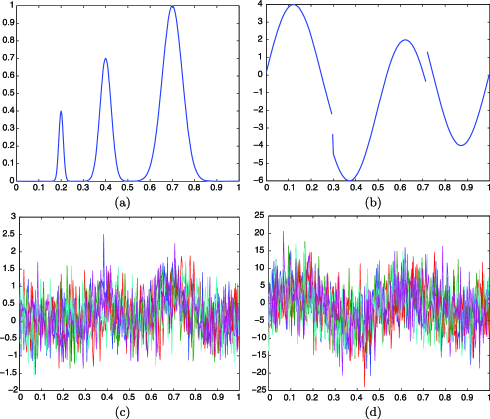
Figure 1: Two test functions $f$. (a) MixtGauss: a mixture of three Gaussians. (b) HeaviSine: a piecewise smooth curve with a discontinuity. Sample of $5$ noisy randomly shifted curves with $n=300$ for (c) MixtGauss and (d) HeaviSine.

To analyze the numerical performance of this estimator, we have considered the following ideal estimator that uses the knowledge of the true random shifts $\theta_{j,p}^{\ast}$ (sampled from the $p$th replication):

$$\tilde{f}_{n,J,p}^{(m)}(t)=\sum_{|k|\leq m}\Biggl{(}\frac{1}{J}\sum_{j=1}^{J}\hat{c}_{k,j,p}^{(1)}e^{i2\pi k\theta_{j,p}^{\ast}}\Biggr{)}\phi_{k}(t),\qquad t\in[0,1].$$

The frequency cut-off $\hat{m}_{\ast}$ for the above ideal estimator is chosen using a model selection procedure based on the knowledge of the true shifts, that is,

$$\hat{m}_{\ast}\in\mathop{\operatorname{argmin}}_{m\in\{1,\ldots,m_{1}\}}\biggl{\{}\int_{0}^{1}\bigl{|}\tilde{f}_{n,J,p}^{(m_{1})}(t)-\tilde{f}_{n,J,p}^{(m)}(t)\bigr{|}^{2}\,dt+\eta\frac{(2m+1)\sigma^{2}}{NJ}\biggr{\}}$$

with $\eta=2.5$.

Then, we define the relative empirical error between the two estimators as

$$R(n,J)=\frac{{{1}/{M}\sum_{p=1}^{M}d^{2}([\hat{f}_{n,J,p}],[f])}}{{{1}/{M}\sum_{p=1}^{M}d^{2}([\tilde{f}_{n,J,p}^{(\hat{m}_{\ast})}],[f])}}.$$

In Figure 2, we display the ratio $R(n,J)$ for various values of $n$ and $J$ and for the two test functions displayed in Figure 1. It can be seen that the function $J\mapsto R(n,J)$ is increasing. This means that the numerical performance of the estimator $\hat{f}_{n,J}$ deteriorates as the number $J$ of curves increases and the number $n$ remains fixed. This is clearly due to the fact that the estimation of the shifts becomes less precise when the dimension $J$ increases. These numerical results are thus consistent with inequality (10) in Theorem 3.1 and our discussion on the rate of convergence of $\hat{f}_{n,J}$ in Section 3. On the other hand, the function $n\mapsto R(n,J)$ is decreasing, and it confirms that the number $n$ of design points is a key parameter to obtain consistent estimators of a mean pattern $f$ with Fréchet means of curves.

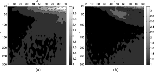
Figure 2: Relative empirical error $R(n,J)$ for various values of $n$ (vertical axis) and $J$ (horizontal axis) over $M=100$ replications: (a) MixtGauss, (b) HeaviSine.

Appendix: Proof of the main results

Throughout the proofs, we repeatedly use the following lemma which follows immediately from Lemma 1.8 in MR2724359 .

Lemma .1.

If $f\in\tilde{W}_{s}(A,c_{*})$, then there exists a constant $A_{0}>0$ only depending on $A$ and $s$ such that

$$\max_{-{N}/{2}\leq k<{N}/{2}}\bigl{|}\bar{c}_{k,j}^{(p)}-c_{k}e^{-i2\pi k\theta_{j}^{\ast}}\bigr{|}\leq A_{0}N^{-s+1/2},\qquad p\in\{0,1\}$$

for all $1\leq j\leq J$.

.1 Proof of Theorem 3.1

For legibility, we will write $\mathbb{E}=\mathbb{E}^{g}$, that is, we omit the dependency on $g$ of the expectation. The proof is divided in several lemmas. Let $\|\cdot\|$ denote the standard Euclidean norm in $\mathbb{R}^{J}$. First, we derive upper bounds on the second, fourth and sixth moments of $\|\hat{\theta}^{0}-\theta^{0}\|$. The following upper bound on the second moment is weaker than the result that we plan to prove. It only gives the consistency of $\hat{\theta}^{0}$, and we will need some additional arguments to get the announced rate of convergence (10).

Lemma .2.

Let $N\geq 2$, $J\geq 1$ and $1\leq k_{0}\leq N/2$. We assume that Assumptions 1 and 2 are satisfied, and we suppose that $s>3/2$. Then, we have the following upper bounds, for any $f\in\tilde{W}_{s}(A,c_{*})$:

$$\frac{1}{J}\mathbb{E}\bigl{(}\bigl{\|}\hat{\theta}^{0}-\theta^{0}\bigr{\|}^{2}\bigr{)} \leq C_{1}\frac{k_{0}^{1/2}}{n^{1/2}},$$ (17)

$$\frac{1}{J}\mathbb{E}\bigl{(}\bigl{\|}\hat{\theta}^{0}-\theta^{0}\bigr{\|}^{4}\bigr{)} \leq C_{2}\frac{k_{0}J}{n}$$ (18)

and

$$\frac{1}{J}\mathbb{E}\bigl{(}\bigl{\|}\hat{\theta}^{0}-\theta^{0}\bigr{\|}^{6}\bigr{)}\leq C_{3}\frac{k_{0}^{3/2}J^{2}}{n^{3/2}},$$ (19)

where $C_{1},C_{2}$ and $C_{3}$ are positive constants that only depend on $A,s,c_{*},\sigma^{2}$ and $\kappa$.

Let $f\in\tilde{W}_{s}(A,c_{*})$. Since $\hat{\theta}^{0}=(\hat{\theta}_{1}^{0},\ldots,\hat{\theta}_{J}^{0})$ is a minimizer of $M_{n}$, it follows that

$$M\bigl{(}\hat{\theta}^{0}\bigr{)}-M\bigl{(}\theta^{0}\bigr{)}\leq 2\sup_{\theta\in\Theta_{\kappa}}\bigl{|}M_{n}(\theta)-M(\theta)\bigr{|}.$$

Therefore, by Proposition 3.1, we get

$$\frac{1}{J}\mathbb{E}\bigl{\|}\hat{\theta}^{0}-\theta^{0}\bigr{\|}^{2} \leq 2C^{-1}(c_{*},\kappa)\mathbb{E}\Bigl{(}\sup_{\theta\in\Theta_{\kappa}}\bigl{|}M_{n}(\theta)-M(\theta)\bigr{|}\Bigr{)},$$ (20)

$$\frac{1}{J}\mathbb{E}\bigl{\|}\hat{\theta}^{0}-\theta^{0}\bigr{\|}^{4} \leq 4C^{-2}(c_{*},\kappa)J\mathbb{E}\Bigl{(}\sup_{\theta\in\Theta_{\kappa}}\bigl{|}M_{n}(\theta)-M(\theta)\bigr{|}^{2}\Bigr{)}$$ (21)

and

$$\frac{1}{J}\mathbb{E}\bigl{\|}\hat{\theta}^{0}-\theta^{0}\bigr{\|}^{6}\leq 8C^{-3}(c_{*},\kappa)J^{2}\mathbb{E}\Bigl{(}\sup_{\theta\in\Theta_{\kappa}}\bigl{|}M_{n}(\theta)-M(\theta)\bigr{|}^{3}\Bigr{)},$$ (22)

where we have set $C(c_{*},\kappa)=4\pi^{2}c_{*}^{2}\cos(8\pi\kappa)$.

Let $\theta\in\Theta_{\kappa}$ and note that $M_{n}(\theta)$ can be decomposed as

$$M_{n}(\theta)=\bar{M}(\theta)+Q(\theta)+L(\theta),$$ (23)

where

$$\bar{M}(\theta) = \frac{1}{J}\sum_{j=1}^{J}\sum_{|k|\leq k_{0}}\Biggl{|}\bar{c}_{k,j}^{(0)}e^{2ik\pi\theta_{j}}-\frac{1}{J}\sum_{j^{\prime}=1}^{J}\bar{c}_{k,j^{\prime}}^{(0)}e^{2ik\pi\theta_{j^{\prime}}}\Biggr{|}^{2},$$

$$Q(\theta) = \frac{1}{NJ}\sum_{j=1}^{J}\sum_{|k|\leq k_{0}}\Biggl{|}z_{k,j}^{(0)}e^{2ik\pi\theta_{j}}-\frac{1}{J}\sum_{j^{\prime}=1}^{J}z_{k,j^{\prime}}^{(0)}e^{2ik\pi\theta_{j^{\prime}}}\Biggr{|}^{2}$$

and

$$L(\theta) = \frac{2}{J\sqrt{N}}\sum_{j=1}^{J}\sum_{|k|\leq k_{0}}\Re\Biggl{[}\Biggl{(}\bar{c}_{k,j}^{(0)}e^{2ik\pi\theta_{j}}-\frac{1}{J}\sum_{j^{\prime}=1}^{J}\bar{c}_{k,j^{\prime}}^{(0)}e^{2ik\pi\theta_{j^{\prime}}}\Biggr{)}$$

$$\hskip 84.0pt{}\times\Biggl{(}\overline{z_{k,j}^{(0)}e^{2ik\pi\theta_{j}}-\frac{1}{J}\sum_{j^{\prime}=1}^{J}z_{k,j^{\prime}}^{(0)}e^{2ik\pi\theta_{j^{\prime}}}}\Biggr{)}\Biggr{]}.$$

Using Lemma .1, it follows that, for any $\theta\in\Theta_{\kappa}$,

$$\bigl{|}\bar{M}(\theta)-M(\theta)\bigr{|}$$

$$\qquad\leq\frac{1}{J}\sum_{j=1}^{J}\sum_{|k|\leq k_{0}}\Biggl{|}\bigl{|}\bar{c}_{k,j}^{(0)}\bigr{|}+\frac{1}{J}\sum_{j^{\prime}=1}^{J}\bigl{|}\bar{c}_{k,j^{\prime}}^{(0)}\bigr{|}+2|c_{k}|\Biggr{|}$$

$$\hskip 61.0pt\qquad{}\times\Biggl{|}\bigl{(}\bar{c}_{k,j}^{(0)}-c_{k}e^{-2ik\pi\theta_{j}^{\ast}}\bigr{)}e^{2ik\pi\theta_{j}}$$

$$\hskip 77.0pt\qquad{}-\frac{1}{J}\sum_{j^{\prime}=1}^{J}\bigl{(}\bar{c}_{k,j^{\prime}}^{(0)}-c_{k}e^{-2ik\pi\theta_{j^{\prime}}^{\ast}}\bigr{)}e^{2ik\pi\theta_{j^{\prime}}}\Biggr{|}$$

$$\qquad\leq 2A_{0}N^{-s+1/2}\sum_{|k|\leq k_{0}}\bigl{(}4|c_{k}|+2A_{0}N^{-s+1/2}\bigr{)}$$

$$\qquad\leq 8A_{0}N^{-s+1/2}(2k_{0}+1)^{1/2}\sqrt{\sum_{|k|\leq k_{0}}|c_{k}|^{2}}+4A_{0}^{2}(2k_{0}+1)N^{-2s+1}.$$

Hence, there exists a positive constant $C$ that only depends on $A$ and $s$ such that

$$\sup_{\theta\in\Theta_{\kappa}}\bigl{|}\bar{M}(\theta)-M(\theta)\bigr{|}\leq Ck_{0}^{1/2}N^{-s+1/2}.$$ (24)

Now, note that $Q(\theta)\leq\frac{\sigma^{2}}{NJ}Z$ with $Z=\sum_{|k|\leq k_{0}}\sum_{j=1}^{J}|z_{k,j}^{(0)}/\sigma|^{2}$ for any $\theta\in\Theta_{\kappa}$. Thus, it follows that

$$\mathbb{E}\sup_{\theta\in\Theta_{\kappa}}\bigl{|}Q(\theta)\bigr{|}\leq\sigma^{2}(2k_{0}+1)N^{-1}$$ (25)

and

$$\mathbb{E}\sup_{\theta\in\Theta_{\kappa}}\bigl{|}Q(\theta)\bigr{|}^{2}\leq 2\sigma^{4}(2k_{0}+1)^{2}N^{-2}.$$ (26)

By Jensen’s inequality, we get

$$\mathbb{E}Z^{3/2}\leq\bigl{(}\mathbb{E}Z^{2}\bigr{)}^{3/4},$$

and since $\mathbb{E}Z^{2}\leq 2J^{2}(2k_{0}+1)^{2}$, we obtain

$$\mathbb{E}\sup_{\theta\in\Theta_{\kappa}}\bigl{|}Q(\theta)\bigr{|}^{3/2}\leq 8^{1/4}\frac{\sigma^{3}}{N^{3/2}}(2k_{0}+1)^{3/2}.$$ (27)

Finally, using $\mathbb{E}Z^{3}\leq 6J^{3}(2k_{0}+1)^{3}$, we have

$$\mathbb{E}\sup_{\theta\in\Theta_{\kappa}}\bigl{|}Q(\theta)\bigr{|}^{3}\leq 6\frac{\sigma^{6}}{N^{3}}(2k_{0}+1)^{3}.$$ (28)

By Cauchy–Schwarz’s inequality,

$$L(\theta)\leq 2\sqrt{\bar{M}(\theta)}\sqrt{Q(\theta)}.$$ (29)

Thanks to Lemma .1, we get

$$\bar{M}(\theta)\leq\frac{1}{J}\sum_{|k|\leq k_{0}}\sum_{j=1}^{J}\bigl{|}\bar{c}_{k,j}^{(0)}\bigr{|}^{2}\leq\sum_{|k|\leq k_{0}}|c_{k}|^{2}+A_{0}^{2}N^{-2s+1}(2k_{0}+1).$$

Thus, it follows from (25), (26), (27) and (29) that there exists a positive constant $C^{\prime}$, only depending on $A$, $s$ and $\sigma^{2}$, such that

$$\mathbb{E}\sup_{\theta\in\Theta_{\kappa}}\bigl{|}L(\theta)\bigr{|} \leq C^{\prime}k_{0}^{1/2}N^{-1/2},$$ (30)

$$\mathbb{E}\sup_{\theta\in\Theta_{\kappa}}\bigl{|}L(\theta)\bigr{|}^{2} \leq {C^{\prime}}^{2}k_{0}N^{-1}$$ (31)

and

$$\mathbb{E}\sup_{\theta\in\Theta_{\kappa}}\bigl{|}L(\theta)\bigr{|}^{3}\leq{C^{\prime}}^{3}k_{0}^{3/2}N^{-3/2}.$$ (32)

Since $s>3/2$, we obtain, by inequalities (24), (25) and (30),

$$\mathbb{E}\Bigl{(}\sup_{\theta\in\Theta_{\kappa}}\bigl{|}M_{n}(\theta)-M(\theta)\bigr{|}\Bigr{)}\leq C^{\prime}_{1}k_{0}^{1/2}N^{-1/2},$$

by inequalities (24), (26) and (31),

$$\mathbb{E}\Bigl{(}\sup_{\theta\in\Theta_{\kappa}}\bigl{|}M_{n}(\theta)-M(\theta)\bigr{|}^{2}\Bigr{)}\leq C^{\prime}_{2}k_{0}N^{-1},$$

and by inequalities (24), (28) and (32),

$$\mathbb{E}\Bigl{(}\sup_{\theta\in\Theta_{\kappa}}\bigl{|}M_{n}(\theta)-M(\theta)\bigr{|}^{3}\Bigr{)}\leq C^{\prime}_{3}k_{0}^{3/2}N^{-3/2},$$

where $C^{\prime}_{1},C^{\prime}_{2}$ and $C^{\prime}_{3}$ are positive constants that only depend on $A,s$ and $\sigma^{2}$. Combined with inequalities (20), (21) and (22), the announced result follows from the above upper bounds.

In order to prove Theorem 3.1, we divide the rest of the proof in the three following steps. In the sequel of this section, we always assume that the hypotheses of Theorem 3.1 are satisfied, and we use the decomposition of $M_{n}(\theta)$ as defined in (23).

Step 1: there exists some positive constant $C_{1}$ that only depends on $c_{*}$ such that

$$\frac{n}{J}\bigl{\|}\hat{\theta}^{0}-\theta^{0}\bigr{\|}^{2}$$

$$\qquad\leq C_{1}\Bigl{(}nJ\bigl{\|}\nabla M_{n}\bigl{(}\theta^{0}\bigr{)}\bigr{\|}^{2}$$ (33)

$$\hskip 48.0pt{}+nJ\sup_{\theta\in\mathcal{U}_{\kappa}}\bigl{\|}\nabla^{2}M_{n}(\theta)-\nabla^{2}M\bigl{(}\theta^{0}\bigr{)}\bigr{\|}^{2}_{\mathrm{op}}\bigl{\|}\hat{\theta}^{0}-\theta^{0}\bigr{\|}^{2}\Bigr{)},$$

where $\nabla$ and $\nabla^{2}$ denote the gradient and the Hessian operators, respectively, and where we have set

$$\mathcal{U}_{\kappa}=\bigl{\{}\theta\in\Theta_{\kappa}\mbox{ such that }\bigl{\|}\theta-\theta^{0}\bigr{\|}\leq\bigl{\|}\hat{\theta}^{0}-\theta^{0}\bigr{\|}\bigr{\}}$$

and, for any $J\times J$ matrix $B$, the operator norm $\|B\|_{\mathrm{op}}$ is defined by

$$\|B\|_{\mathrm{op}}=\sup_{\theta\in\mathbb{R}^{J}\setminus\{0\}}\frac{\|B\theta\|}{\|\theta\|}.$$

Step 2: there exists some positive constant $C_{2}$ that only depends on $A,s$ and $\sigma^{2}$ such that

$$nJ\mathbb{E}\bigl{\|}\nabla M_{n}\bigl{(}\theta^{0}\bigr{)}\bigr{\|}^{2}\leq C_{2}\biggl{(}1+\frac{k_{0}^{3}}{n}\biggr{)}.$$ (34)

Step 3: there exists some positive constant $C_{3}$ that only depends on $A,s,\kappa$, $c_{*}$ and $\sigma^{2}$ such that

$$nJ\mathbb{E}\Bigl{(}\sup_{\theta\in\mathcal{U}_{\kappa}}\bigl{\|}\nabla^{2}M_{n}(\theta)-\nabla^{2}M\bigl{(}\theta^{0}\bigr{)}\bigr{\|}^{2}_{\mathrm{op}}\bigl{\|}\hat{\theta}^{0}-\theta^{0}\bigr{\|}^{2}\Bigr{)}$$

(35)

$$\qquad\leq C_{3}\biggl{(}1+\frac{k_{0}^{5}}{n^{{1}/{2}}}\biggr{)}\frac{k_{0}^{{3}/{2}}J^{3}}{n^{{1}/{2}}}.$$

The result announced in Theorem 3.1 follows from inequalities (.1), (34) and (.1).

.1.1 Proof of Step 1

The gradients of $\bar{M}(\theta),Q(\theta)$ and $L(\theta)$ follow from easy computations. We have, for any $1\leq\ell\leq J$,

$$\frac{\partial}{\partial\theta_{\ell}}\bar{M}(\theta) = \frac{4\pi}{J^{2}}\sum_{|k|\leq k_{0}}k\Re\Biggl{[}i\overline{\bar{c}_{k,\ell}^{(0)}e^{2ik\pi\theta_{\ell}}}\Biggl{(}\sum_{j=1}^{J}\bar{c}_{k,j}^{(0)}e^{2ik\pi\theta_{j}}\Biggr{)}\Biggr{]},$$ (36)

$$\frac{\partial}{\partial\theta_{\ell}}Q(\theta) = \frac{4\pi}{NJ^{2}}\sum_{|k|\leq k_{0}}k\Re\Biggl{[}i\overline{z_{k,\ell}^{(0)}e^{2ik\pi\theta_{\ell}}}\Biggl{(}\sum_{j=1,j\neq\ell}^{J}z_{k,j}^{(0)}e^{2ik\pi\theta_{j}}\Biggr{)}\Biggr{]}$$ (37)

and

$$\frac{\partial}{\partial\theta_{\ell}}L(\theta) = -\frac{4\pi}{J^{2}\sqrt{N}}\sum_{|k|\leq k_{0}}k\Im\Biggl{[}\overline{z_{k,\ell}^{(0)}e^{2ik\pi\theta_{\ell}}}\Biggl{(}\sum_{j=1,j\neq\ell}^{J}\bar{c}_{k,j}^{(0)}e^{2ik\pi\theta_{j}}\Biggr{)}$$

$$\hskip 86.0pt{}-\bar{c}_{k,\ell}^{(0)}e^{2ik\pi\theta_{\ell}}\Biggl{(}\overline{\sum_{j=1,j\neq\ell}^{J}z_{k,j}^{(0)}e^{2ik\pi\theta_{j}}}\Biggr{)}\Biggr{]}.$$

Similarly, we can compute the Hessians of these functions as follows, for $1\leq\ell,\ell^{\prime}\leq J$, if $\ell\neq\ell^{\prime}$,

$$\frac{\partial^{2}}{\partial\theta_{\ell^{\prime}}\,\partial\theta_{\ell}}\bar{M}(\theta) = -\frac{8\pi^{2}}{J^{2}}\sum_{|k|\leq k_{0}}k^{2}\Re\bigl{[}\overline{\bar{c}_{k,\ell}^{(0)}}\bar{c}_{k,\ell^{\prime}}^{(0)}e^{2ik\pi(\theta_{\ell^{\prime}}-\theta_{\ell})}\bigr{]},$$ (39)

$$\frac{\partial^{2}}{\partial\theta_{\ell^{\prime}}\,\partial\theta_{\ell}}Q(\theta) = -\frac{8\pi^{2}}{NJ^{2}}\sum_{|k|\leq k_{0}}k^{2}\Re\bigl{[}\overline{z_{k,\ell}^{(0)}}z_{k,\ell^{\prime}}^{(0)}e^{2ik\pi(\theta_{\ell^{\prime}}-\theta_{\ell})}\bigr{]}$$ (40)

and

$$\frac{\partial^{2}}{\partial\theta_{\ell^{\prime}}\,\partial\theta_{\ell}}L(\theta) = -\frac{8\pi^{2}}{J^{2}\sqrt{N}}\sum_{|k|\leq k_{0}}k^{2}\Re\bigl{[}\bar{c}_{k,\ell^{\prime}}^{(0)}\overline{z_{k,\ell}^{(0)}}e^{2ik\pi(\theta_{\ell^{\prime}}-\theta_{\ell})}$$

$$\hskip 88.0pt{}+\bar{c}_{k,\ell}^{(0)}\overline{z_{k,\ell^{\prime}}^{(0)}}e^{2ik\pi(\theta_{\ell}-\theta_{\ell^{\prime}})}\bigr{]},$$

and if $\ell=\ell^{\prime}$,

$$\frac{\partial^{2}}{\partial\theta_{\ell}\,\partial\theta_{\ell}}\bar{M}(\theta) = \frac{8\pi^{2}}{J^{2}}\sum_{|k|\leq k_{0}}k^{2}\Re\Biggl{[}\overline{\bar{c}_{k,\ell}^{(0)}e^{2ik\pi\theta_{\ell}}}\Biggl{(}\sum_{j=1,j\neq\ell}^{J}\bar{c}_{k,j}^{(0)}e^{2ik\pi\theta_{j}}\Biggr{)}\Biggr{]},$$ (42)

$$\frac{\partial^{2}}{\partial\theta_{\ell}\,\partial\theta_{\ell}}Q(\theta) = \frac{8\pi^{2}}{NJ^{2}}\sum_{|k|\leq k_{0}}k^{2}\Re\Biggl{[}\overline{z_{k,\ell}^{(0)}e^{2ik\pi\theta_{\ell}}}\Biggl{(}\sum_{j=1,j\neq\ell}^{J}z_{k,j}^{(0)}e^{2ik\pi\theta_{j}}\Biggr{)}\Biggr{]}$$ (43)

and

$$\frac{\partial^{2}}{\partial\theta_{\ell}\,\partial\theta_{\ell}}L(\theta) = \frac{8\pi^{2}}{J^{2}\sqrt{N}}\sum_{|k|\leq k_{0}}k^{2}\Re\Biggl{[}\bar{c}_{k,\ell}^{(0)}e^{2ik\pi\theta_{\ell}}\Biggl{(}\overline{\sum_{j=1,j\neq\ell}^{J}z_{k,j}^{(0)}e^{2ik\pi\theta_{j}}}\Biggr{)}$$

$$\hskip 81.0pt{}+\overline{z_{k,\ell}^{(0)}e^{2ik\pi\theta_{\ell}}}\Biggl{(}\sum_{j=1,j\neq\ell}^{J}\bar{c}_{k,j}^{(0)}e^{2ik\pi\theta_{j}}\Biggr{)}\Biggr{]}.$$

Using the fact that $\hat{\theta}^{0}\in\Theta_{\kappa}$ is a minimizer of $M_{n}$, so $\nabla M_{n}(\hat{\theta}^{0})=0$, a Taylor expansion of $\theta\mapsto\nabla M_{n}(\theta)$ with an integral form of the remainder term leads to

$$0=\nabla M_{n}\bigl{(}\theta^{0}\bigr{)}+\int_{0}^{1}\nabla^{2}M_{n}\bigl{(}\bar{\theta}(t)\bigr{)}\bigl{(}\hat{\theta}^{0}-\theta^{0}\bigr{)}\,dt,$$ (45)

where, for any $t\in[0,1]$, we have set

$$\bar{\theta}(t)=\theta^{0}+t\bigl{(}\hat{\theta}^{0}-\theta^{0}\bigr{)}\in\mathcal{U}_{\kappa}.$$

Thus, we have

$$\nabla^{2}M\bigl{(}\theta^{0}\bigr{)}\bigl{(}\hat{\theta}^{0}-\theta^{0}\bigr{)}$$

(46)

$$\qquad=-\nabla M_{n}\bigl{(}\theta^{0}\bigr{)}-\int_{0}^{1}\bigl{(}\nabla^{2}M_{n}\bigl{(}\bar{\theta}(t)\bigr{)}-\nabla^{2}M\bigl{(}\theta^{0}\bigr{)}\bigr{)}\bigl{(}\hat{\theta}^{0}-\theta^{0}\bigr{)}\,dt.$$

It follows from similar computations as we did for $\bar{M}$ that

$$\nabla^{2}M\bigl{(}\theta^{0}\bigr{)}=\frac{8\pi^{2}}{J}\sum_{|k|\leq k_{0}}k^{2}|c_{k}|^{2}\biggl{(}I_{J}-\frac{1}{J}\mathbh{1}_{J}\biggr{)},$$

where $I_{J}$ is the $J\times J$ identity matrix and $\mathbh{1}_{J}$ denotes the $J\times J$ matrix with all entries equal to one. Therefore, using the fact that $\sum_{j=1}^{J}(\hat{\theta}_{j}^{0}-\theta_{j}^{0})=0$, we obtain

$$\bigl{\|}\nabla^{2}M\bigl{(}\theta^{0}\bigr{)}\bigl{(}\hat{\theta}^{0}-\theta^{0}\bigr{)}\bigr{\|}^{2}=\frac{64\pi^{4}}{J^{2}}\biggl{(}\sum_{|k|\leq k_{0}}k^{2}|c_{k}|^{2}\biggr{)}^{2}\bigl{\|}\hat{\theta}^{0}-\theta^{0}\bigr{\|}^{2},$$

and it shows that there exists a constant $C>0$ that only depends on $c_{*}$ such that

$$\bigl{\|}\nabla^{2}M\bigl{(}\theta^{0}\bigr{)}\bigl{(}\hat{\theta}^{0}-\theta^{0}\bigr{)}\bigr{\|}^{2}\geq C\frac{1}{J^{2}}\bigl{\|}\hat{\theta}^{0}-\theta^{0}\bigr{\|}^{2}.$$ (47)

Then, inequality (.1) follows from (.1.1) and (47).

.1.2 Proof of Step 2

By using Lemma .1, for any $1\leq k\leq k_{0}$ and $1\leq\ell\leq J$, we can expand

$$\bar{c}_{k,\ell}^{(0)}e^{2ik\pi\theta_{\ell}^{0}}=c_{k}e^{2ik\pi(\theta_{\ell}^{0}-\theta_{\ell}^{\ast})}+\alpha_{k,\ell}e^{2ik\pi\theta_{\ell}^{0}}$$

with $|\alpha_{k,\ell}|\leq A_{0}N^{-s+1/2}$. Because, for any $j$, $\theta^{0}_{j}-\theta^{*}_{j}=\bar{\theta}_{J}$ does not depend on $j$, we have

$$\Biggl{|}\Re\Biggl{[}i\overline{\bar{c}_{k,\ell}^{(0)}e^{2ik\pi\theta_{\ell}}}\Biggl{(}\sum_{j=1}^{J}\bar{c}_{k,j}^{(0)}e^{2ik\pi\theta_{j}}\Biggr{)}\Biggr{]}\Biggr{|}\leq A_{0}JN^{-s+1/2}\bigl{(}2|c_{k}|+A_{0}N^{-s+1/2}\bigr{)}.$$

Thus, by equation (36) and using Cauchy–Schwarz’s inequality, we obtain

$$\biggl{|}\frac{\partial}{\partial\theta_{\ell}}\bar{M}\bigl{(}\theta^{0}\bigr{)}\biggr{|}^{2} \leq \frac{32\pi^{2}}{J^{2}}(2k_{0}+1)A_{0}^{2}N^{-2s+1}\sum_{|k|\leq k_{0}}k^{2}\bigl{(}4|c_{k}|^{2}+A_{0}^{2}N^{-2s+1}\bigr{)}$$

$$\leq \frac{64\pi^{2}}{J^{2}}(2k_{0}+1)A_{0}^{2}N^{-2s+1}\bigl{(}A^{2}+A_{0}^{2}k_{0}^{3}N^{-2s+1}\bigr{)}.$$

Thus, there exists a positive constant $C$ that only depends on $A$ and $s$ such that

$$nJ\bigl{\|}\nabla\bar{M}\bigl{(}\theta^{0}\bigr{)}\bigr{\|}^{2}\leq Ck_{0}\bigl{(}1+k_{0}^{3}n^{-2s+1}\bigr{)}n^{-2s+2}.$$ (48)

We now focus on $\nabla Q$ and, by (37), we can obtain

$$\sum_{\ell=1}^{J}\mathbb{E}\biggl{|}\frac{\partial}{\partial\theta_{\ell}}Q\bigl{(}\theta^{0}\bigr{)}\biggr{|}^{2} \leq \frac{16\pi^{2}(J-1)^{2}}{N^{2}J^{4}}\sum_{\ell=1}^{J}\sum_{|k|\leq k_{0}}k^{2}\frac{1}{J-1}\sum_{j=1,j\neq\ell}^{J}\mathbb{E}\bigl{|}z_{k,\ell}^{(0)}\bigr{|}^{2}\bigl{|}z_{k,j}^{(0)}\bigr{|}^{2}$$

$$\leq \frac{32\pi^{2}\sigma^{4}k_{0}^{3}}{N^{2}J}.$$

Hence, we get

$$nJ\mathbb{E}\bigl{\|}\nabla Q\bigl{(}\theta^{0}\bigr{)}\bigr{\|}^{2}\leq\frac{128\pi^{2}\sigma^{4}k_{0}^{3}}{n}.$$ (49)

Finally, we deal with $\nabla L$. Equation (.1.1) and Lemma .1 imply

$$\mathbb{E}\biggl{|}\frac{\partial}{\partial\theta_{\ell}}L(\theta)\biggr{|}^{2} \leq \frac{16\pi^{2}\sigma^{2}}{J^{4}N}\sum_{|k|\leq k_{0}}k^{2}\Biggl{(}\Biggl{|}\sum_{j=1,j\neq\ell}^{J}\bar{c}_{k,j}^{(0)}e^{2ik\pi\theta_{j}}\Biggr{|}^{2}+J\bigl{|}\bar{c}_{k,\ell}^{(0)}\bigr{|}^{2}\Biggr{)}$$

$$\leq \frac{16\pi^{2}\sigma^{2}}{J^{4}N}\sum_{|k|\leq k_{0}}k^{2}\Biggl{(}(J-1)\sum_{j=1,j\neq\ell}^{J}\bigl{|}\bar{c}_{k,j}^{(0)}\bigr{|}^{2}+J\bigl{|}\bar{c}_{k,\ell}^{(0)}\bigr{|}^{2}\Biggr{)}$$

$$\leq \frac{16\pi^{2}\sigma^{2}}{J^{2}N}\sum_{|k|\leq k_{0}}k^{2}\Biggl{(}\frac{1}{J}\sum_{j=1}^{J}\bigl{|}\bar{c}_{k,j}^{(0)}\bigr{|}^{2}\Biggr{)}$$

$$\leq \frac{32\pi^{2}\sigma^{2}}{J^{2}N}\sum_{|k|\leq k_{0}}k^{2}\bigl{(}|c_{k}|^{2}+A_{0}^{2}N^{-2s+1}\bigr{)}.$$

This last inequality leads to

$$nJ\mathbb{E}\bigl{\|}\nabla L\bigl{(}\theta^{0}\bigr{)}\bigr{\|}^{2}\leq 64\pi^{2}\sigma^{2}\bigl{(}A^{2}+2A_{0}^{2}\bigr{)}\bigl{(}1+k_{0}^{3}n^{-2s+1}\bigr{)}.$$ (50)

By combining inequalities (48), (49) and (50), we then obtain inequality (34).

.1.3 Proof of Step 3

We introduce the Frobenius norm $\|B\|_{F}$ defined, for any $J\times J$ matrix $B=[B_{\ell,\ell^{\prime}}]_{1\leq\ell,\ell^{\prime}\leq J}$, as

$$\|B\|_{F}=\sqrt{\sum_{\ell,\ell^{\prime}=1}^{J}B_{\ell,\ell^{\prime}}^{2}}.$$

Moreover, for a self-adjoint matrix $B$, we will use the classical inequalities

$$\|B\|_{\mathrm{op}}\leq\|B\|_{F}\quad\mbox{and}\quad\|B\|_{\mathrm{op}}\leq\max_{1\leq\ell^{\prime}\leq J}\sum_{\ell=1}^{J}|B_{\ell,\ell^{\prime}}|.$$ (51)

In order to prove inequality (.1), we use the following decomposition:

$$\bigl{\|}\nabla^{2}M_{n}(\theta)-\nabla^{2}M\bigl{(}\theta^{0}\bigr{)}\bigr{\|}^{2}_{\mathrm{op}} \leq 4\bigl{(}\bigl{\|}\nabla^{2}\bar{M}(\theta)-\nabla^{2}M(\theta)\bigr{\|}^{2}_{F}$$

$$\hskip 8.0pt{}+\bigl{\|}\nabla^{2}M(\theta)-\nabla^{2}M\bigl{(}\theta^{0}\bigr{)}\bigr{\|}^{2}_{\mathrm{op}}$$

$$\hskip 8.0pt{}+\bigl{\|}\nabla^{2}Q(\theta)\bigr{\|}^{2}_{F}+\bigl{\|}\nabla^{2}L(\theta)\bigr{\|}^{2}_{F}\bigr{)}.$$

We now deal with each term in the above inequality. Hereafter, $\ell$ and $\ell^{\prime}$ always denote two integers in $\{1,\ldots,J\}$.

First, let us consider $\ell\neq\ell^{\prime}$, by (39) and Lemma .1, we get

$$\biggl{|}\frac{\partial^{2}}{\partial\theta_{\ell^{\prime}}\,\partial\theta_{\ell}}\bar{M}(\theta)-\frac{\partial^{2}}{\partial\theta_{\ell^{\prime}}\,\partial\theta_{\ell}}M(\theta)\biggr{|}^{2}$$

$$\qquad=\frac{64\pi^{4}}{J^{4}}\biggl{(}\sum_{|k|\leq k_{0}}k^{2}\Re\bigl{[}\bigl{(}\bar{c}_{k,\ell}^{(0)}\overline{\bar{c}_{k,\ell^{\prime}}^{(0)}}-|c_{k}|^{2}e^{2ik\pi(\theta_{\ell^{\prime}}^{\ast}-\theta_{\ell}^{\ast})}\bigr{)}e^{i2\pi k(\theta_{\ell}-\theta_{\ell^{\prime}})}\bigr{]}\biggr{)}^{2}$$

$$\qquad\leq\frac{64\pi^{4}}{J^{4}}\biggl{(}\sum_{|k|\leq k_{0}}k^{2}\bigl{|}\bar{c}_{k,\ell}^{(0)}\overline{\bar{c}_{k,\ell^{\prime}}^{(0)}}-|c_{k}|^{2}e^{2ik\pi(\theta_{\ell^{\prime}}^{\ast}-\theta_{\ell}^{\ast})}\bigr{|}\biggr{)}^{2}$$

$$\qquad\leq\frac{256\pi^{4}}{J^{4}}\biggl{(}\sum_{|k|\leq k_{0}}k^{2}\bigl{(}A_{0}|c_{k}|N^{-s+1/2}+A_{0}^{2}N^{-2s+1}\bigr{)}\biggr{)}^{2}.$$

In the case of $\ell=\ell^{\prime}$, (42) and Lemma .1 lead to

$$\biggl{|}\frac{\partial^{2}}{\partial\theta_{\ell}\,\partial\theta_{\ell}}\bar{M}(\theta)-\frac{\partial^{2}}{\partial\theta_{\ell}\,\partial\theta_{\ell}}M(\theta)\biggr{|}^{2}$$

$$\qquad\leq\frac{64\pi^{4}}{J^{4}}\Biggl{(}\sum_{|k|\leq k_{0}}k^{2}\sum_{j=1,j\neq\ell}^{J}\bigl{|}\bar{c}_{k,\ell}^{(0)}\overline{\bar{c}_{k,j}^{(0)}}-|c_{k}|^{2}e^{2ik\pi(\theta_{j}^{\ast}-\theta_{\ell}^{\ast})}\bigr{|}\Biggr{)}^{2}$$

$$\qquad\leq\frac{256\pi^{4}}{J^{2}}\biggl{(}\sum_{|k|\leq k_{0}}k^{2}\bigl{(}A_{0}|c_{k}|N^{-s+1/2}+A_{0}^{2}N^{-2s+1}\bigr{)}\biggr{)}^{2}.$$

Therefore, the above inequalities and (17) imply that there exists some positive constant $C_{M}$ that only depends on $A$, $s$, $\kappa$ and $\sigma^{2}$ such that

$$nJ\mathbb{E}\Bigl{(}\sup_{\theta\in\mathcal{U}_{\kappa}}\bigl{\|}\nabla^{2}\bar{M}(\theta)-\nabla^{2}M(\theta)\bigr{\|}^{2}_{F}\bigl{\|}\hat{\theta}^{0}-\theta^{0}\bigr{\|}^{2}\Bigr{)}\leq C_{M}\frac{k_{0}^{6+1/2}J}{n^{2s-3/2}}.$$ (53)

Second, using the fact that $2(1-\cos(t))\leq t^{2}$ for any $t\in\mathbb{R}$, if $\ell\neq\ell^{\prime}$, then we have

$$\biggl{|}\frac{\partial^{2}}{\partial\theta_{\ell^{\prime}}\,\partial\theta_{\ell}}M(\theta)-\frac{\partial^{2}}{\partial\theta_{\ell^{\prime}}\,\partial\theta_{\ell}}M\bigl{(}\theta^{0}\bigr{)}\biggr{|}$$

$$\qquad=\frac{8\pi^{2}}{J^{2}}\biggl{|}\sum_{|k|\leq k_{0}}k^{2}|c_{k}|^{2}\Re\bigl{[}e^{2ik\pi(\theta_{\ell}-\theta_{\ell}^{0}+\theta_{\ell^{\prime}}^{0}-\theta_{\ell^{\prime}})}-1\bigr{]}\biggr{|}$$

$$\qquad\leq\frac{16\pi^{4}}{J^{2}}\biggl{(}\sum_{|k|\leq k_{0}}k^{4}|c_{k}|^{2}\biggr{)}\bigl{|}\theta_{\ell}-\theta_{\ell}^{0}+\theta_{\ell^{\prime}}^{0}-\theta_{\ell^{\prime}}\bigr{|}^{2},$$

and if $\ell=\ell^{\prime}$ then we obtain

$$\biggl{|}\frac{\partial^{2}}{\partial\theta_{\ell}\,\partial\theta_{\ell}}M(\theta)-\frac{\partial^{2}}{\partial\theta_{\ell}\,\partial\theta_{\ell}}M\bigl{(}\theta^{0}\bigr{)}\biggr{|}$$

$$\qquad=\frac{8\pi^{2}}{J^{2}}\Biggl{|}\sum_{|k|\leq k_{0}}k^{2}|c_{k}|^{2}\Re\Biggl{[}\Biggl{(}\sum_{j=1,j\neq\ell}^{J}\bigl{(}e^{2ik\pi(\theta_{\ell}-\theta_{\ell}^{0}-\theta_{j}+\theta_{j}^{0})}-1\bigr{)}\Biggr{)}\Biggr{]}\Biggr{|}$$

$$\qquad\leq\frac{16\pi^{4}}{J^{2}}\biggl{(}\sum_{|k|\leq k_{0}}k^{4}|c_{k}|^{2}\biggr{)}\sum_{j=1,j\neq\ell}^{J}\bigl{|}\theta_{\ell}-\theta_{\ell}^{0}-\theta_{j}+\theta_{j}^{0}\bigr{|}^{2}.$$

Therefore, by (51) and under the condition $s\geq 2$, we get

$$\bigl{\|}\nabla^{2}M(\theta)-\nabla^{2}M\bigl{(}\theta^{0}\bigr{)}\bigr{\|}_{\mathrm{op}} \leq \frac{32\pi^{4}A^{2}}{J^{2}}\max_{1\leq\ell\leq J}\sum_{j=1,j\neq\ell}^{J}\bigl{|}\theta_{\ell}-\theta_{\ell}^{0}-\theta_{j}+\theta_{j}^{0}\bigr{|}^{2}$$

$$\leq \frac{64\pi^{4}A^{2}}{J}\bigl{\|}\theta-\theta^{0}\bigr{\|}^{2}.$$

Thus, by definition of $\mathcal{U}_{\kappa}$ and by (19), we know that there exists some $C_{M}^{\prime}>0$ that only depends on $A$, $s$, $\sigma^{2}$ and $\kappa$ such that

$$nJ\mathbb{E}\Bigl{(}\sup_{\theta\in\mathcal{U}_{\kappa}}\bigl{\|}\nabla^{2}M(\theta)-\nabla^{2}M\bigl{(}\theta^{0}\bigr{)}\bigr{\|}^{2}_{\mathrm{op}}\bigl{\|}\hat{\theta}^{0}-\theta^{0}\bigr{\|}^{2}\Bigr{)}$$

$$\qquad\leq\frac{n(64\pi^{4}A^{2})^{2}}{J}\mathbb{E}\bigl{(}\bigl{\|}\hat{\theta}^{0}-\theta^{0}\bigr{\|}^{6}\bigr{)}$$ (54)

$$\qquad\leq C_{M}^{\prime}\frac{k_{0}^{3/2}J^{2}}{n^{1/2}}.$$

Next, we deal with the term relative to $\|\nabla^{2}Q(\theta)\|_{F}^{2}$. Let us begin by noting that $\|\hat{\theta}^{0}-\theta^{0}\|^{2}\leq 4J\kappa^{2}$. Thus, we have

$$\mathbb{E}\Bigl{(}\sup_{\theta\in\mathcal{U}_{\kappa}}\bigl{\|}\nabla^{2}Q(\theta)\bigr{\|}^{2}_{F}\bigl{\|}\hat{\theta}^{0}-\theta^{0}\bigr{\|}^{2}\Bigr{)}\leq 4J\kappa^{2}\mathbb{E}\Bigl{(}\sup_{\theta\in\mathcal{U}_{\kappa}}\bigl{\|}\nabla^{2}Q(\theta)\bigr{\|}^{2}_{F}\Bigr{)}.$$ (55)

If we take $\ell\neq\ell^{\prime}$, then using (40), we get

$$\biggl{|}\frac{\partial^{2}}{\partial\theta_{\ell^{\prime}}\,\partial\theta_{\ell}}Q(\theta)\biggr{|}^{2}\leq\frac{64\pi^{4}}{N^{2}J^{4}}\biggl{(}\sum_{|k|\leq k_{0}}k^{2}\bigl{|}z_{k,\ell}^{(0)}\bigr{|}\bigl{|}z_{k,\ell^{\prime}}^{(0)}\bigr{|}\biggr{)}^{2}$$

and if $\ell=\ell^{\prime}$, then by (43), we have

$$|\frac{\partial^{2}}{\partial\theta_{\ell}^{2}}Q(\theta)\biggr{|}^{2} \leq \frac{64\pi^{4}}{N^{2}J^{4}}\Biggl{(}\sum_{|k|\leq k_{0}}k^{2}\bigl{|}z_{k,\ell}^{(0)}\bigr{|}\Biggl{|}\sum_{j=1,j\neq\ell}^{J}z_{k,j}^{(0)}e^{i2\pi k\theta_{j}}\Biggr{|}\Biggr{)}^{2}$$

$$\leq \frac{64\pi^{4}}{N^{2}J^{3}}\sum_{j=1,j\neq\ell}^{J}\biggl{(}\sum_{|k|\leq k_{0}}k^{2}\bigl{|}z_{k,\ell}^{(0)}\bigr{|}\bigl{|}z_{k,j}^{(0)}\bigr{|}\biggr{)}^{2}.$$

Hence, the Cauchy–Schwarz inequality leads to the following upper bound:

$$\mathbb{E}\Bigl{(}\sup_{\theta\in\mathcal{U}_{\kappa}}\bigl{\|}\nabla^{2}Q(\theta)\bigr{\|}^{2}_{F}\Bigr{)}$$

$$\qquad\leq\frac{128\pi^{4}}{N^{2}J^{3}}\mathbb{E}\sum_{\ell=1}^{J}\sum_{\ell^{\prime}=1,\ell^{\prime}\neq\ell}^{J}\biggl{(}\sum_{|k|\leq k_{0}}k^{2}\bigl{|}z_{k,\ell}^{(0)}\bigr{|}\bigl{|}z_{k,\ell^{\prime}}^{(0)}\bigr{|}\biggr{)}^{2}$$

$$\qquad\leq\frac{128\pi^{4}}{N^{2}J^{3}}\sum_{\ell=1}^{J}\sum_{\ell^{\prime}=1,\ell^{\prime}\neq\ell}^{J}\mathbb{E}\biggl{(}\sum_{|k|\leq k_{0}}k^{2}\bigl{|}z_{k,\ell}^{(0)}\bigr{|}^{2}\biggr{)}\mathbb{E}\biggl{(}\sum_{|k|\leq k_{0}}k^{2}\bigl{|}z_{k,\ell^{\prime}}^{(0)}\bigr{|}^{2}\biggr{)}$$

$$\qquad\leq\frac{512\pi^{4}\sigma^{4}k_{0}^{6}}{N^{2}J}.$$

Combining this bound with (55) gives us some $C_{Q}>0$ that only depends on $\kappa$ and $\sigma^{2}$ such that

$$nJ\mathbb{E}\Bigl{(}\sup_{\theta\in\mathcal{U}_{\kappa}}\bigl{\|}\nabla^{2}Q(\theta)\bigr{\|}^{2}_{F}\bigl{\|}\hat{\theta}^{0}-\theta^{0}\bigr{\|}^{2}\Bigr{)}\leq C_{Q}\frac{k_{0}^{6}J}{n}.$$ (56)

Finally, we focus on the term concerning $\|\nabla^{2}L(\theta)\|^{2}_{F}$. By the Cauchy–Schwarz inequality and (18), we have

$$\mathbb{E}\Bigl{(}\sup_{\theta\in\mathcal{U}_{\kappa}}\bigl{\|}\nabla^{2}L(\theta)\bigr{\|}^{2}_{F}\bigl{\|}\hat{\theta}^{0}-\theta^{0}\bigr{\|}^{2}\Bigr{)}$$

$$\qquad\leq\sqrt{\mathbb{E}\Bigl{(}\sup_{\theta\in\mathcal{U}_{\kappa}}\bigl{\|}\nabla^{2}L(\theta)\bigr{\|}^{4}_{F}\Bigr{)}}\sqrt{\mathbb{E}\bigl{(}\bigl{\|}\hat{\theta}^{0}-\theta^{0}\bigr{\|}^{4}\bigr{)}}$$ (57)

$$\qquad\leq\sqrt{\mathbb{E}\Bigl{(}\sup_{\theta\in\mathcal{U}_{\kappa}}\bigl{\|}\nabla^{2}L(\theta)\bigr{\|}^{4}_{F}\Bigr{)}}\sqrt{C_{2}\frac{k_{0}J^{2}}{n}}.$$

Using Lemma .1 and (.1.1), if $\ell\neq\ell^{\prime}$, we obtain

$$\biggl{|}\frac{\partial^{2}}{\partial\theta_{\ell^{\prime}}\,\partial\theta_{\ell}}L(\theta)\biggr{|}^{2} \leq \frac{64\pi^{4}}{J^{4}N}\biggl{(}\sum_{|k|\leq k_{0}}k^{2}\bigl{(}\bigl{|}\bar{c}_{k,\ell}^{(0)}\overline{z_{k,\ell^{\prime}}^{(0)}}\bigr{|}+\bigl{|}\bar{c}_{k,\ell^{\prime}}^{(0)}\overline{z_{k,\ell}^{(0)}}\bigr{|}\bigr{)}\biggr{)}^{2}$$

$$\leq \frac{64\pi^{4}}{J^{4}N}\biggl{(}\sum_{|k|\leq k_{0}}k^{2}\bigl{(}|c_{k}|+A_{0}N^{-s+{1}/{2}}\bigr{)}\bigl{(}\bigl{|}z_{k,\ell}^{(0)}\bigr{|}+\bigl{|}z_{k,\ell^{\prime}}^{(0)}\bigr{|}\bigr{)}\biggr{)}^{2}$$

and, by (.1.1), if $\ell=\ell^{\prime}$, we get

$$\biggl{|}\frac{\partial^{2}}{\partial\theta_{\ell}\,\partial\theta_{\ell}}L(\theta)\biggr{|}^{2}$$

$$\qquad\leq\frac{64\pi^{4}}{J^{4}N}\Biggl{(}\sum_{|k|\leq k_{0}}k^{2}\Biggl{(}\bigl{|}\bar{c}_{k,\ell}^{(0)}\bigr{|}\Biggl{(}\sum_{j=1,j\neq\ell}^{J}\bigl{|}z_{k,j}^{(0)}\bigr{|}\Biggr{)}+\bigl{|}z_{k,\ell}^{(0)}\bigr{|}\Biggl{(}\sum_{j=1,j\neq\ell}^{J}|\bar{c}_{k,j}^{(0)}|\Biggr{)}\Biggr{)}\Biggr{)}^{2}$$

$$\qquad\leq\frac{64\pi^{4}}{J^{4}N}\Biggl{(}\sum_{|k|\leq k_{0}}k^{2}\Biggl{(}\bigl{(}|c_{k}|+A_{0}N^{-s+1/2}\bigr{)}\Biggl{(}J\bigl{|}z_{k,\ell}^{(0)}\bigr{|}+\sum_{j=1,j\neq\ell}^{J}\bigl{|}z_{k,j}^{(0)}\bigr{|}\Biggr{)}\Biggr{)}\Biggr{)}^{2}.$$

Hence, we bound the expectation in (.1.3) from above,

$$\mathbb{E}\Bigl{(}\sup_{\theta\in\mathcal{U}_{\kappa}}\bigl{\|}\nabla^{2}L(\theta)\bigr{\|}^{4}_{F}\Bigr{)}$$

$$\qquad\leq\frac{4096\pi^{8}}{J^{4}N^{2}}\mathbb{E}\Biggl{(}\Biggl{[}J\Biggl{(}\sum_{|k|\leq k_{0}}k^{2}\bigl{(}|c_{k}|+A_{0}N^{-s+1/2}\bigr{)}\sum_{j=1}^{J}\bigl{|}z_{k,j}^{(0)}\bigr{|}\Biggr{)}^{2}$$

$$\hskip 56.0pt\qquad\quad{}+\frac{4}{J}\sum_{\ell=1}^{J}\biggl{(}\sum_{|k|\leq k_{0}}k^{2}\bigl{(}|c_{k}|+A_{0}N^{-s+1/2}\bigr{)}\bigl{|}z_{k,\ell}^{(0)}\bigr{|}\biggr{)}^{2}\Biggr{]}^{2}\Biggr{)}$$

$$\qquad\leq\frac{4\times 4096\pi^{8}}{J^{2}N^{2}}\mathbb{E}\Biggl{(}\Biggl{(}\sum_{|k|\leq k_{0}}k^{2}\bigl{(}|c_{k}|+A_{0}N^{-s+1/2}\bigr{)}\sum_{j=1}^{J}\bigl{|}z_{k,j}^{(0)}\bigr{|}\Biggr{)}^{4}\Biggr{)}$$

$$\qquad\leq\frac{4\times 4096\pi^{8}}{N^{2}}\biggl{(}\sum_{|k|\leq k_{0}}k^{4}\bigl{(}|c_{k}|+A_{0}N^{-s+1/2}\bigr{)}^{2}\biggr{)}^{2}\mathbb{E}\Biggl{(}\Biggl{(}\sum_{|k|\leq k_{0}}\sum_{j=1}^{J}\bigl{|}z_{k,j}^{(0)}\bigr{|}^{2}\Biggr{)}^{2}\Biggr{)}$$

$$\qquad\leq\frac{168\times 4096\pi^{8}\sigma^{4}J^{2}k_{0}^{2}}{N^{2}}\biggl{(}\sum_{|k|\leq k_{0}}k^{4}\bigl{(}|c_{k}|+A_{0}N^{-s+1/2}\bigr{)}^{2}\biggr{)}^{2}.$$

Therefore, there exists some constant $C_{L}^{\prime}>0$ that only depends on $A$, $s$ and $\sigma^{2}$ such that

$$\mathbb{E}\Bigl{(}\sup_{\theta\in\mathcal{U}_{\kappa}}\bigl{\|}\nabla^{2}L(\theta)\bigr{\|}^{4}_{F}\Bigr{)}\leq C_{L}^{\prime}\frac{k_{0}^{2}J^{2}}{n^{2}}\biggl{(}1+\frac{k_{0}^{5}}{n^{2s-1}}\biggr{)}^{2}.$$ (58)

Using (.1.3) and (58), we know that there exists some constant $C_{L}>0$ that only depends on $c_{*}$, $\kappa$, $A$, $s$ and $\sigma^{2}$ such that

$$nJ\mathbb{E}\Bigl{(}\sup_{\theta\in\mathcal{U}_{\kappa}}\bigl{\|}\nabla^{2}L(\theta)\bigr{\|}^{2}_{F}\bigl{\|}\hat{\theta}^{0}-\theta^{0}\bigr{\|}^{2}\Bigr{)}\leq C_{L}\frac{k_{0}^{3/2}J^{3}}{\sqrt{n}}\biggl{(}1+\frac{k_{0}^{5}}{n^{2s-1}}\biggr{)}.$$ (59)

Finally, we use (53), (.1.3), (56) and (59) with (.1.3) to get (.1).

.2 Proof of Theorem 3.2

Let us assume that $f\in\tilde{W}_{s}(A,c_{*})$. We bound the distance between $f$ and $\hat{f}_{n,J}$ from above,

$$d^{2}\bigl{(}[f],[\hat{f}_{n,J}]\bigr{)} = \inf_{\theta\in[-1/2,1/2]}\int_{0}^{1}\bigl{|}f(t-\theta)-\hat{f}_{n,J}(t)\bigr{|}^{2}\,dt$$

$$\leq 2d^{2}\bigl{(}[f],\bigl{[}\bar{f}^{(m_{1})}\bigr{]}\bigr{)}+2\int_{0}^{1}\bigl{|}\bar{f}^{(m_{1})}(t)-\hat{f}_{n,J}(t)\bigr{|}^{2}\,dt.$$

Taking the expectation according to the distribution of $Y^{(1)}$ on both sides and using (3.2) leads to

$$\mathbb{E}^{(1)}\bigl{[}d^{2}\bigl{(}[f],[\hat{f}_{n,J}]\bigr{)}\bigr{]}$$

$$\qquad\leq 2d^{2}\bigl{(}[f],\bigl{[}\bar{f}^{(m_{1})}\bigr{]}\bigr{)}$$

$$\qquad\quad{}+2C(\eta)\min_{m\in\{1,\ldots,m_{1}\}}\biggl{\{}\int_{0}^{1}\bigl{|}\bar{f}^{(m_{1})}(t)-\bar{f}^{(m)}(t)\bigr{|}^{2}\,dt+\frac{2(m+1)\sigma^{2}}{NJ}\biggr{\}}$$ (60)

$$\qquad\leq 2d^{2}\bigl{(}[f],\bigl{[}\bar{f}^{(m_{1})}\bigr{]}\bigr{)}$$

$$\qquad\quad{}+2C(\eta)\min_{m\in\{1,\ldots,m_{1}\}}\Biggl{\{}\sum_{m<|k|\leq m_{1}}\Biggl{|}\frac{1}{J}\sum_{j=1}^{J}\bar{c}^{(1)}_{k,j}e^{i2\pi k\hat{\theta}^{0}_{j}}\Biggr{|}^{2}+\frac{2(m+1)\sigma^{2}}{NJ}\Biggr{\}}.$$

Let $\bar{\theta}_{J}=(\theta^{*}_{1}+\cdots+\theta^{*}_{J})/J$, we recall that $\theta^{0}=\theta^{*}-\bar{\theta}_{J}$. We begin by upper bounding the first term. Thanks to Jensen’s inequality, we obtain

$$d^{2}\bigl{(}[f],\bigl{[}\bar{f}^{(m_{1})}\bigr{]}\bigr{)} \leq \int_{0}^{1}\bigl{|}f(t-\bar{\theta}_{J})-\bar{f}^{(m_{1})}(t)\bigr{|}^{2}\,dt$$

$$\leq \sum_{|k|>m_{1}}|c_{k}|^{2}+\sum_{|k|\leq m_{1}}\Biggl{|}c_{k}e^{-i2\pi k\bar{\theta}_{J}}-\frac{1}{J}\sum_{j=1}^{J}\bar{c}^{(1)}_{k,j}e^{i2\pi k\hat{\theta}^{0}_{j}}\Biggr{|}^{2}$$

$$\leq \sum_{|k|>m_{1}}|c_{k}|^{2}+\sum_{|k|\leq m_{1}}\frac{1}{J}\sum_{j=1}^{J}\bigl{|}c_{k}e^{-i2\pi k\bar{\theta}_{J}}-\bar{c}^{(1)}_{k,j}e^{i2\pi k\hat{\theta}^{0}_{j}}\bigr{|}^{2}.$$

Since $f\in\tilde{W}_{s}(A,c_{*})$, we easily upper bound the bias part

$$\sum_{|k|>m_{1}}|c_{k}|^{2}\leq A|m_{1}|^{-2s}.$$ (62)

To deal with the other part, we split it into two sums,

$$\frac{1}{J}\sum_{j=1}^{J}\bigl{|}c_{k}e^{-i2\pi k\bar{\theta}_{J}}-\bar{c}^{(1)}_{k,j}e^{i2\pi k\hat{\theta}^{0}_{j}}\bigr{|}^{2}$$

$$\qquad\leq\frac{2}{J}\sum_{j=1}^{J}\bigl{|}c_{k}e^{-i2\pi k\bar{\theta}_{J}}-c_{k}e^{i2\pi k(\hat{\theta}^{0}_{j}-\theta^{*}_{j})}\bigr{|}^{2}$$

$$\qquad\quad{}+\frac{2}{J}\sum_{j=1}^{J}\bigl{|}c_{k}e^{i2\pi k(\hat{\theta}^{0}_{j}-\theta^{*}_{j})}-\bar{c}^{(1)}_{k,j}e^{i2\pi k\hat{\theta}^{0}_{j}}\bigr{|}^{2}$$ (63)

$$\qquad\leq\frac{2|c_{k}|^{2}}{J}\sum_{j=1}^{J}\bigl{|}1-e^{i2\pi k(\hat{\theta}^{0}_{j}-\theta^{0}_{j})}\bigr{|}^{2}+\frac{2}{J}\sum_{j=1}^{J}\bigl{|}\bar{c}^{(1)}_{k,j}-c_{k}e^{-i2\pi k\theta^{*}_{j}}\bigr{|}^{2}$$

$$\qquad\leq\frac{8\pi^{2}k^{2}|c_{k}|^{2}}{J}\sum_{j=1}^{J}\bigl{(}\hat{\theta}^{0}_{j}-\theta^{0}_{j}\bigr{)}^{2}+2A_{0}^{2}N^{-2s+1},$$

where the last inequality follows from Lemma .1 and from $2(1-\cos t)\leq t^{2}$, $t\in\mathbb{R}$. Combining (.2), (62) and (.2), we get, for any $g\in\mathcal{G}^{\kappa}$,

$$\mathbb{E}^{g}\bigl{[}d^{2}\bigl{(}[f],\bigl{[}\bar{f}^{(m_{1})}\bigr{]}\bigr{)}\bigr{]} \leq A|m_{1}|^{-2s}+2A_{0}^{2}(2m_{1}+1)N^{-2s+1}$$

$${}+8\pi^{2}\biggl{(}\sum_{|k|\leq m_{1}}k^{2}|c_{k}|^{2}\biggr{)}\mathbb{E}^{g}\Biggl{[}\frac{1}{J}\sum_{j=1}^{J}\bigl{(}\hat{\theta}^{0}_{j}-\theta^{0}_{j}\bigr{)}^{2}\Biggr{]}.$$

We now focus on the second term in (.2). Let $\alpha_{k,j}=c_{k}e^{-i2\pi k\theta^{*}_{j}}-\bar{c}^{(1)}_{k,j}$, using Jensen’s inequality and Lemma .1, for any $m\in\{1,\ldots,m_{1}\}$, we have

$$\sum_{m<|k|\leq m_{1}}\Biggl{|}\frac{1}{J}\sum_{j=1}^{J}\bar{c}^{(1)}_{k,j}e^{i2\pi k\hat{\theta}^{0}_{j}}\Biggr{|}^{2} \leq \sum_{m<|k|\leq m_{1}}\frac{1}{J}\sum_{j=1}^{J}\bigl{|}c_{k}e^{-i2\pi k\theta^{*}_{j}}+\alpha_{k,j}\bigr{|}^{2}$$

$$\leq 2\sum_{|k|>m}|c_{k}|^{2}+\frac{2}{J}\sum_{m<|k|\leq m_{1}}\sum_{j=1}^{J}|\alpha_{k,j}|^{2}$$

$$\leq 2Am^{-2s}+4A_{0}^{2}m_{1}N^{-2s+1}.$$

Let us consider $m_{\ast}$ such that

$$m_{\ast}=\biggl{\lfloor}\biggl{(}\frac{nJ}{c}\biggr{)}^{1/(2s+1)}\biggr{\rfloor},$$

where $c$ is the constant such that $J\leq cn^{\alpha}$. Note that such a choice is allowed because it is such that $m_{\ast}\in\{1,\ldots,m_{1}\}$ since $n\geq 21$, $s>3/2$, $\alpha\in(0,1/6]$ and $c\in(0,1)$. In particular, such a choice leads to the following upper bound:

$$\min_{m\in\{1,\ldots,m_{1}\}}\Biggl{\{}\sum_{m<|k|\leq m_{1}}\Biggl{|}\frac{1}{J}\sum_{j=1}^{J}\bar{c}^{(1)}_{k,j}e^{i2\pi k\hat{\theta}^{0}_{j}}\Biggr{|}^{2}+\frac{2(m+1)\sigma^{2}}{NJ}\Biggr{\}}$$

$$\qquad\leq 4A_{0}^{2}m_{1}N^{-2s+1}+\frac{2\sigma^{2}}{NJ}+2\min_{m\in\{1,\ldots,m_{1}\}}\biggl{\{}Am^{-2s}+\frac{m\sigma^{2}}{NJ}\biggr{\}}$$

$$\qquad\leq 4A_{0}^{2}m_{1}N^{-2s+1}+\frac{2\sigma^{2}}{NJ}$$ (65)

$$\qquad\quad{}+2\biggl{(}\frac{A}{2}c^{2s/(2s+1)}+2\sigma^{2}c^{2s/(2s+1)}\biggr{)}(nJ)^{-2s/(2s+1)}$$

$$\qquad\leq 4A_{0}^{2}m_{1}N^{-2s+1}+\bigl{(}1+\bigl{(}A+4\sigma^{2}\bigr{)}c^{2s/(2s+1)}\bigr{)}(nJ)^{-2s/(2s+1)}.$$

Putting (.2) and (.2) in (.2) leads to, for any $g\in\mathcal{G}^{\kappa}$,

$$\mathcal{R}_{g}(\hat{f}_{n,J},f) \leq A|m_{1}|^{-2s}+4A_{0}^{2}\bigl{(}\bigl{(}1+C(\eta)\bigr{)}m_{1}+1\bigr{)}N^{-2s+1}$$

$${}+8\pi^{2}\biggl{(}\sum_{|k|\leq m_{1}}k^{2}|c_{k}|^{2}\biggr{)}\mathbb{E}^{g}\Biggl{[}\frac{1}{J}\sum_{j=1}^{J}\bigl{(}\hat{\theta}^{0}_{j}-\theta^{0}_{j}\bigr{)}^{2}\Biggr{]}$$

$${}+C(\eta)\bigl{(}1+\bigl{(}A+4\sigma^{2}\bigr{)}c^{2s/(2s+1)}\bigr{)}(nJ)^{-2s/(2s+1)},$$

that completes the proof using the fact that $m_{1}=\lfloor N/2\rfloor-1$.

.3 Proof of Theorem 4.1

The arguments that we use to derive this result are based on Assouad’s cube lemma; see, for example, MR2724359 . This lemma is classically used in nonparametric statistics to derive lower bounds on a risk. We will show that one can construct a set of functions $\mathcal{F}_{0}\subset\tilde{W}_{s}(A,c_{*})$ such that there exists a constant $C>0$ (only depending on $A$, $s$, $c_{*}$ and $\sigma^{2}$) such that, for any large enough $n$ and $J$,

$$\qquad\mathcal{R}_{n,J}\bigl{(}\tilde{W}_{s}(A,c_{*}),\mathcal{G}^{\kappa}\bigr{)}\geq\inf_{\hat{f}_{n,J}}\sup_{g\in\mathcal{G}^{\kappa}}\sup_{f\in\mathcal{F}_{0}}\mathcal{R}_{g}(\hat{f}_{n,J},f)\geq C(nJ)^{-{2s}/{(2s+1)}},$$ (66)

where $\hat{f}_{n,J}$ denote some estimator of $f$. For the sake of legibility, we assume in the sequel that $c_{*}=1$. Let

$$\mathcal{F}_{0}=\biggl{\{}f_{w}\dvtx t\in[0,1]\mapsto\sqrt{\mu_{n,J}}\sum_{k\in K_{n,J}}w_{k}\phi_{k}(t),w_{k}\in\{-1,1\},w_{-k}=w_{k}\biggr{\}},$$

where $K_{n,J}=\{k\in\mathbb{Z},0<|k|\leq D_{n,J}\}$, $\mu_{n,J}$ is a positive real and $D_{n,J}$ is a positive integer that will be specified below. Let us introduce the notation $\Omega=\{-1,1\}^{D_{n,J}}$ and note that any function $f_{w}\in\mathcal{F}_{0}$ is parametrized by a unique element $w\in\Omega$. Under the condition

$$\mu_{n,J}=cD_{n,J}^{-2s-1}\qquad\mbox{with }c\leq A,$$ (67)

it can easily be checked that $\mathcal{F}_{0}\subset\tilde{W}_{s}(A,c_{*})$. In what follows, $D_{n,J}$ is chosen as the largest integer smaller that $(nJ)^{{1}/{(2s+1)}}$. Hereafter, $\mathbb{E}_{w}^{g}$ will denote the expectation with respect to the distribution $\mathbb{P}_{w}^{g}$ of the random vector $(Y_{\ell,j})_{1\leq\ell\leq n,1\leq j\leq J}\in\mathbb{R}^{nJ}$ in model (3) under the hypothesis that $f=f_{w}$ and the assumption that the shifts are i.i.d. random variables with density $g\in\mathcal{G}^{\kappa}$. Note that for any $g\in\mathcal{G}^{\kappa}$

$$\sup_{f\in\mathcal{F}_{0}}\mathcal{R}_{g}(\hat{f}_{n,J},f) = \sup_{f\in\mathcal{F}_{0}}\mathbb{E}\biggl{[}\inf_{\theta\in[0,1]}\biggl{(}\int_{0}^{1}\bigl{|}\hat{f}_{n,J}(t-\theta)-f(t)\bigr{|}^{2}\,dt\biggr{)}\biggr{]}$$

$$\geq \frac{1}{|\Omega|}\sum_{w\in\Omega}\mathbb{E}^{g}_{w}\biggl{[}\inf_{\theta\in[0,1]}\biggl{(}\int_{0}^{1}\bigl{|}\hat{f}_{n,J}(t-\theta)-f_{w}(t)\bigr{|}^{2}\,dt\biggr{)}\biggr{]}$$

$$\geq \frac{1}{|\Omega|}\sum_{w\in\Omega}\mathbb{E}^{g}_{w}\biggl{[}\inf_{\theta\in[0,1]}\sum_{k\in K_{n,J}}\bigl{|}\hat{c}_{k}e^{-2ik\pi\theta}-\sqrt{\mu_{n,J}}w_{k}\bigr{|}^{2}\biggr{]},$$

where $\hat{c}_{k}=\int_{0}^{1}\hat{f}_{n,J}(t)\overline{\phi_{k}(t)}\,dt$ is the $k$th Fourier coefficient of $\hat{f}_{n,J}$. Now, we consider, for $k\in K_{n,J}$ and $\theta\in[0,1]$,

$$\hat{w}_{k,\theta}\in\mathop{\operatorname{argmin}}_{v\in\{-1,1\}}\bigl{|}\hat{c}_{k}e^{-2ik\pi\theta}-\sqrt{\mu_{n,J}}v\bigr{|}.$$

We have the inequality

$$\bigl{|}\sqrt{\mu_{n,J}}\hat{w}_{k,\theta}-\sqrt{\mu_{n,J}}w_{k}\bigr{|} \leq \bigl{|}\hat{c}_{k}e^{-2ik\pi\theta}-\sqrt{\mu_{n,J}}\hat{w}_{k,\theta}\bigr{|}$$

$${}+\bigl{|}\hat{c}_{k}e^{-2ik\pi\theta}-\sqrt{\mu_{n,J}}w_{k}\bigr{|}$$

$$\leq 2\bigl{|}\hat{c}_{k}e^{-2ik\pi\theta}-\sqrt{\mu_{n,J}}w_{k}\bigr{|}$$

that implies

$$\sup_{f\in\mathcal{F}_{0}}\mathcal{R}_{g}(\hat{f}_{n,J},f) \geq \frac{\mu_{n,J}}{4|\Omega|}\sum_{k\in K_{n,J}}\sum_{w\in\Omega}\mathbb{E}^{g}_{w}\Bigl{[}\inf_{\theta\in[0,1]}\bigl{(}|\hat{w}_{k,\theta}-w_{k}|^{2}\bigr{)}\Bigr{]}.$$

For $w\in\Omega$ and $k\in K_{n,J}$, we define $w^{(k)}\in\Omega$ such that, for any $\ell\neq k$, $w^{(k)}_{\ell}=w_{\ell}$ and $w^{(k)}_{k}=-w_{k}$. Then it follows that

$$\sup_{f\in\mathcal{F}_{0}}\mathcal{R}_{g}(\hat{f}_{n,J},f)\geq\frac{\mu_{n,J}}{4|\Omega|}\sum_{k\in K_{n,J}}\sum_{w\in\Omega|w_{k}=1}R_{k},$$ (68)

where we have set

$$R_{k}=\mathbb{E}^{g}_{w}\Bigl{[}\inf_{\theta\in[0,1]}\bigl{(}|\hat{w}_{k,\theta}-w_{k}|^{2}\bigr{)}\Bigr{]}+\mathbb{E}^{g}_{w^{(k)}}\Bigl{[}\inf_{\theta\in[0,1]}\bigl{(}|\hat{w}_{k,\theta}+w_{k}|^{2}\bigr{)}\Bigr{]}.$$

Let $\theta^{\ast}=(\theta_{1}^{\ast},\ldots,\theta_{J}^{\ast})$, we introduce the notation $\mathbb{E}_{w}^{\theta^{\ast}}$ to denote expectation with respect to the distribution $\mathbb{P}_{w}^{\theta^{\ast}}$ of the random vector $(Y_{\ell,j})_{1\leq\ell\leq n,1\leq j\leq J}\in\mathbb{R}^{nJ}$ in model (1) conditionally to $\theta_{1}^{\ast},\ldots,\theta_{J}^{\ast}$. Hence, using this notation, we have

$$R_{k}=\int_{[-{1}/{2},{1}/{2}]^{J}}R_{k}\bigl{(}\theta^{\ast}\bigr{)}g\bigl{(}\theta_{1}^{\ast}\bigr{)}\cdots g\bigl{(}\theta_{J}^{\ast}\bigr{)}\,d\theta_{1}^{\ast}\cdots\,d\theta_{J}^{\ast},$$ (69)

where

$$R_{k}\bigl{(}\theta^{\ast}\bigr{)}=\mathbb{E}^{\theta^{\ast}}_{w}\Bigl{[}\inf_{\theta\in[0,1]}\bigl{(}|\hat{w}_{k,\theta}-w_{k}|^{2}\bigr{)}\Bigr{]}+\mathbb{E}^{\theta^{\ast}}_{w^{(k)}}\Bigl{[}\inf_{\theta\in[0,1]}\bigl{(}|\hat{w}_{k,\theta}+w_{k}|^{2}\bigr{)}\Bigr{]}.$$

Now, note that for any $0<\delta<1$,

$$R_{k}\bigl{(}\theta^{\ast}\bigr{)} = \mathbb{E}^{\theta^{\ast}}_{w}\biggl{[}\inf_{\theta\in[0,1]}\bigl{(}|\hat{w}_{k,\theta}-w_{k}|^{2}\bigr{)}+\inf_{\theta\in[0,1]}\bigl{(}|\hat{w}_{k,\theta}+w_{k}|^{2}\bigr{)}\frac{d\mathbb{P}^{\theta^{\ast}}_{w^{(k)}}}{d\mathbb{P}^{\theta^{\ast}}_{w}}(Y)\biggr{]}$$

$$\geq 4\mathbb{E}^{g}_{w}\min\biggl{(}1,\frac{d\mathbb{P}^{\theta^{\ast}}_{w^{(k)}}}{d\mathbb{P}^{\theta^{\ast}}_{w}}(Y)\biggr{)}\geq 4\delta\mathbb{P}^{\theta^{\ast}}_{w}\biggl{(}\frac{d\mathbb{P}^{\theta^{\ast}}_{w^{(k)}}}{d\mathbb{P}^{\theta^{\ast}}_{w}}(Y)\geq\delta\biggr{)},$$

where $Y\in\mathbb{R}^{nJ}$ is the random vector obtained from the concatenation of the observations from model (3) under the hypothesis $f=f_{w}$ and conditionally to $\theta_{1}^{\ast},\ldots,\theta_{J}^{\ast}$. Because $w_{k}=1$, we know that

$$\log\frac{d\mathbb{P}^{\theta^{\ast}}_{w^{(k)}}}{d\mathbb{P}^{\theta^{\ast}}_{w}}(Y)=-\frac{2}{\sigma^{2}}\sum_{j=1}^{J}\sum_{\ell=1}^{n}\mu_{n,J}\bigl{|}\phi_{k}\bigl{(}t_{\ell}-\theta_{j}^{\ast}\bigr{)}\bigr{|}^{2}+\sqrt{\mu_{n,J}}\varepsilon_{\ell,j}\phi_{k}\bigl{(}t_{\ell}-\theta_{j}^{\ast}\bigr{)}.$$

Therefore, $\log\frac{d\mathbb{P}^{\theta^{\ast}}_{w^{(k)}}}{d\mathbb{P}^{\theta^{\ast}}_{w}}(Y)$ is a random variable that is normally distributed with mean $-\frac{2}{\sigma^{2}}nJ\mu_{n,J}$ and variance $\frac{4}{\sigma^{2}}nJ\mu_{n,J}$. Now, since $D_{nJ}$ is the largest integer smaller than $(nJ)^{{1}/{(2s+1)}}$, it follows from equation (67) that, for any $n$ and $J$ large enough,

$$0\leq nJ\mu_{n,J}\leq 2A.$$

Thus, there exists $0<\delta<1$ and a constant $c_{\delta}>0$ (only depending on $A$, $\sigma^{2}$ and $\delta$) such that

$$\mathbb{P}^{\theta^{\ast}}_{w}\biggl{(}\frac{d\mathbb{P}^{\theta^{\ast}}_{w^{(k)}}}{d\mathbb{P}^{\theta^{\ast}}_{w}}(Y)\geq\delta\biggr{)}\geq c_{\delta}.$$

Combining this inequality with (68), (69) and (.3) leads to

$$\sup_{f\in\mathcal{F}_{0}}\mathcal{R}_{g}(\hat{f}_{n,J},f)\geq\frac{4\delta\mu_{n,J}}{|\Omega|}\sum_{k\in K_{n,J}}\sum_{w\in\Omega|w_{k}=1}c_{\delta}\geq\delta c_{\delta}\mu_{n,J}D_{n,J}.$$ (71)

Since $\mu_{n,J}=cD_{n,J}^{-2s-1}$ and $D_{n,J}\leq(nJ)^{{1}/{(2s+1)}}$, it follows that

$$\mu_{n,J}D_{n,J}=cD_{n,J}^{-2s}\geq c(nJ)^{-{2s}/{(2s+1)}},$$

which combined with (71) proves inequality (66) and completes the proof of Theorem 4.1.

References

- (1) {barticle}[mr] \bauthor\bsnmAfsari, \bfnmBijan\binitsB. (\byear2011). \btitleRiemannian center of mass: Existence, uniqueness, and convexity. \bjournalProc. Amer. Math. Soc. \bvolume139 \bpages655–673. \biddoi=10.1090/S0002-9939-2010-10541-5, issn=0002-9939, mr=2736346 \bptokimsref \endbibitem
- (2) {barticle}[mr] \bauthor\bsnmBhattacharya, \bfnmRabi\binitsR. and \bauthor\bsnmPatrangenaru, \bfnmVic\binitsV. (\byear2003). \btitleLarge sample theory of intrinsic and extrinsic sample means on manifolds. I. \bjournalAnn. Statist. \bvolume31 \bpages1–29. \biddoi=10.1214/aos/1046294456, issn=0090-5364, mr=1962498 \bptokimsref \endbibitem
- (3) {barticle}[mr] \bauthor\bsnmBhattacharya, \bfnmRabi\binitsR. and \bauthor\bsnmPatrangenaru, \bfnmVic\binitsV. (\byear2005). \btitleLarge sample theory of intrinsic and extrinsic sample means on manifolds. II. \bjournalAnn. Statist. \bvolume33 \bpages1225–1259. \biddoi=10.1214/009053605000000093, issn=0090-5364, mr=2195634 \bptokimsref \endbibitem
- (4) {barticle}[mr] \bauthor\bsnmBigot, \bfnmJérémie\binitsJ. (\byear2006). \btitleLandmark-based registration of curves via the continuous wavelet transform. \bjournalJ. Comput. Graph. Statist. \bvolume15 \bpages542–564. \biddoi=10.1198/106186006X133023, issn=1061-8600, mr=2291263 \bptokimsref \endbibitem
- (5) {barticle}[mr] \bauthor\bsnmBigot, \bfnmJérémie\binitsJ. and \bauthor\bsnmCharlier, \bfnmBenjamin\binitsB. (\byear2011). \btitleOn the consistency of Fréchet means in deformable models for curve and image analysis. \bjournalElectron. J. Stat. \bvolume5 \bpages1054–1089. \biddoi=10.1214/11-EJS633, issn=1935-7524, mr=2836769 \bptokimsref \endbibitem
- (6) {barticle}[mr] \bauthor\bsnmBigot, \bfnmJérémie\binitsJ. and \bauthor\bsnmGadat, \bfnmSébastien\binitsS. (\byear2010). \btitleA deconvolution approach to estimation of a common shape in a shifted curves model. \bjournalAnn. Statist. \bvolume38 \bpages2422–2464. \biddoi=10.1214/10-AOS800, issn=0090-5364, mr=2676894 \bptokimsref \endbibitem
- (7) {barticle}[mr] \bauthor\bsnmBigot, \bfnmJérémie\binitsJ., \bauthor\bsnmLoubes, \bfnmJean-Michel\binitsJ.-M. and \bauthor\bsnmVimond, \bfnmMyriam\binitsM. (\byear2012). \btitleSemiparametric estimation of shifts on compact Lie groups for image registration. \bjournalProbab. Theory Related Fields \bvolume152 \bpages425–473. \biddoi=10.1007/s00440-010-0327-2, issn=0178-8051, mr=2892953 \bptnotecheck year\bptokimsref \endbibitem
- (8) {bmisc}[auto:STB—2013/04/11—08:11:48] \bauthor\bsnmCharlier, \bfnmB.\binitsB. (\byear2013). \bhowpublishedNecessary and sufficient condition for the existence of a Fréchet mean on the circle. ESAIM Probab. Stat. To appear. \bptokimsref \endbibitem
- (9) {barticle}[mr] \bauthor\bsnmFan, \bfnmJianqing\binitsJ. (\byear1991). \btitleOn the optimal rates of convergence for nonparametric deconvolution problems. \bjournalAnn. Statist. \bvolume19 \bpages1257–1272. \biddoi=10.1214/aos/1176348248, issn=0090-5364, mr=1126324 \bptokimsref \endbibitem
- (10) {barticle}[mr] \bauthor\bsnmFréchet, \bfnmMaurice\binitsM. (\byear1948). \btitleLes éléments aléatoires de nature quelconque dans un espace distancié. \bjournalAnn. Inst. H. Poincaré \bvolume10 \bpages215–310. \bidmr=0027464 \bptokimsref \endbibitem
- (11) {barticle}[mr] \bauthor\bsnmGamboa, \bfnmFabrice\binitsF., \bauthor\bsnmLoubes, \bfnmJean-Michel\binitsJ.-M. and \bauthor\bsnmMaza, \bfnmElie\binitsE. (\byear2007). \btitleSemi-parametric estimation of shifts. \bjournalElectron. J. Stat. \bvolume1 \bpages616–640. \biddoi=10.1214/07-EJS026, issn=1935-7524, mr=2369028 \bptokimsref \endbibitem
- (12) {barticle}[mr] \bauthor\bsnmGlasbey, \bfnmC. A.\binitsC. A. and \bauthor\bsnmMardia, \bfnmK. V.\binitsK. V. (\byear2001). \btitleA penalized likelihood approach to image warping. \bjournalJ. R. Stat. Soc. Ser. B Stat. Methodol. \bvolume63 \bpages465–514. \biddoi=10.1111/1467-9868.00295, issn=1369-7412, mr=1858399 \bptokimsref \endbibitem
- (13) {barticle}[mr] \bauthor\bsnmGoodall, \bfnmColin\binitsC. (\byear1991). \btitleProcrustes methods in the statistical analysis of shape. \bjournalJ. Roy. Statist. Soc. Ser. B \bvolume53 \bpages285–339. \bidissn=0035-9246, mr=1108330 \bptokimsref \endbibitem
- (14) {bbook}[mr] \bauthor\bsnmGrenander, \bfnmUlf\binitsU. (\byear1993). \btitleGeneral Pattern Theory: A Mathematical Study of Regular Structures. \bpublisherThe Clarendon Press Oxford Univ. Press, \blocationNew York. \bidmr=1270904 \bptokimsref \endbibitem
- (15) {bbook}[mr] \bauthor\bsnmGrenander, \bfnmUlf\binitsU. and \bauthor\bsnmMiller, \bfnmMichael I.\binitsM. I. (\byear2007). \btitlePattern Theory: From Representation to Inference. \bpublisherOxford Univ. Press, \blocationOxford. \bidmr=2285439 \bptokimsref \endbibitem
- (16) {bmisc}[auto:STB—2013/04/11—08:11:48] \bauthor\bsnmHotz, \bfnmT.\binitsT. and \bauthor\bsnmHuckemann, \bfnmS.\binitsS. (\byear2011). \bhowpublishedIntrinsic means on the circle: Uniqueness, locus and asymptotics. Available at arXiv:\arxivurl1108.2141. \bptokimsref \endbibitem
- (17) {barticle}[mr] \bauthor\bsnmHuckemann, \bfnmStephan F.\binitsS. F. (\byear2011). \btitleIntrinsic inference on the mean geodesic of planar shapes and tree discrimination by leaf growth. \bjournalAnn. Statist. \bvolume39 \bpages1098–1124. \biddoi=10.1214/10-AOS862, issn=0090-5364, mr=2816349 \bptokimsref \endbibitem
- (18) {barticle}[mr] \bauthor\bsnmKendall, \bfnmDavid G.\binitsD. G. (\byear1984). \btitleShape manifolds, Procrustean metrics, and complex projective spaces. \bjournalBull. Lond. Math. Soc. \bvolume16 \bpages81–121. \biddoi=10.1112/blms/16.2.81, issn=0024-6093, mr=0737237 \bptokimsref \endbibitem
- (19) {barticle}[mr] \bauthor\bsnmKneip, \bfnmAlois\binitsA. and \bauthor\bsnmGasser, \bfnmTheo\binitsT. (\byear1988). \btitleConvergence and consistency results for self-modeling nonlinear regression. \bjournalAnn. Statist. \bvolume16 \bpages82–112. \biddoi=10.1214/aos/1176350692, issn=0090-5364, mr=0924858 \bptokimsref \endbibitem
- (20) {barticle}[mr] \bauthor\bsnmKneip, \bfnmAlois\binitsA. and \bauthor\bsnmGasser, \bfnmTheo\binitsT. (\byear1992). \btitleStatistical tools to analyze data representing a sample of curves. \bjournalAnn. Statist. \bvolume20 \bpages1266–1305. \biddoi=10.1214/aos/1176348769, issn=0090-5364, mr=1186250 \bptokimsref \endbibitem
- (21) {bbook}[mr] \bauthor\bsnmMassart, \bfnmPascal\binitsP. (\byear2007). \btitleConcentration Inequalities and Model Selection. \bseriesLecture Notes in Math. \bvolume1896. \bpublisherSpringer, \blocationBerlin. \bidmr=2319879 \bptokimsref \endbibitem
- (22) {barticle}[mr] \bauthor\bsnmMcKilliam, \bfnmRobby G.\binitsR. G., \bauthor\bsnmQuinn, \bfnmBarry G.\binitsB. G. and \bauthor\bsnmClarkson, \bfnmI. Vaughan L.\binitsI. V. L. (\byear2012). \btitleDirection estimation by minimum squared arc length. \bjournalIEEE Trans. Signal Process. \bvolume60 \bpages2115–2124. \biddoi=10.1109/TSP.2012.2186444, issn=1053-587X, mr=2954196 \bptokimsref \endbibitem
- (23) {barticle}[mr] \bauthor\bsnmPensky, \bfnmMarianna\binitsM. and \bauthor\bsnmVidakovic, \bfnmBrani\binitsB. (\byear1999). \btitleAdaptive wavelet estimator for nonparametric density deconvolution. \bjournalAnn. Statist. \bvolume27 \bpages2033–2053. \biddoi=10.1214/aos/1017939249, issn=0090-5364, mr=1765627 \bptokimsref \endbibitem
- (24) {bbook}[mr] \bauthor\bsnmRamsay, \bfnmJ. O.\binitsJ. O. and \bauthor\bsnmSilverman, \bfnmB. W.\binitsB. W. (\byear2002). \btitleApplied Functional Data Analysis: Methods and Case Studies. \bpublisherSpringer, \blocationNew York. \biddoi=10.1007/b98886, mr=1910407 \bptokimsref \endbibitem
- (25) {barticle}[mr] \bauthor\bsnmRønn, \bfnmBirgitte B.\binitsB. B. (\byear2001). \btitleNonparametric maximum likelihood estimation for shifted curves. \bjournalJ. R. Stat. Soc. Ser. B Stat. Methodol. \bvolume63 \bpages243–259. \biddoi=10.1111/1467-9868.00283, issn=1369-7412, mr=1841413 \bptokimsref \endbibitem
- (26) {barticle}[mr] \bauthor\bsnmTang, \bfnmRong\binitsR. and \bauthor\bsnmMüller, \bfnmHans-Georg\binitsH.-G. (\byear2008). \btitlePairwise curve synchronization for functional data. \bjournalBiometrika \bvolume95 \bpages875–889. \biddoi=10.1093/biomet/asn047, issn=0006-3444, mr=2461217 \bptokimsref \endbibitem
- (27) {barticle}[mr] \bauthor\bsnmTrigano, \bfnmThomas\binitsT., \bauthor\bsnmIsserles, \bfnmUri\binitsU. and \bauthor\bsnmRitov, \bfnmYa’acov\binitsY. (\byear2011). \btitleSemiparametric curve alignment and shift density estimation for biological data. \bjournalIEEE Trans. Signal Process. \bvolume59 \bpages1970–1984. \biddoi=10.1109/TSP.2011.2113179, issn=1053-587X, mr=2816476 \bptokimsref \endbibitem
- (28) {barticle}[mr] \bauthor\bsnmTrouvé, \bfnmAlain\binitsA. and \bauthor\bsnmYounes, \bfnmLaurent\binitsL. (\byear2005). \btitleLocal geometry of deformable templates. \bjournalSIAM J. Math. Anal. \bvolume37 \bpages17–59 (electronic). \biddoi=10.1137/S0036141002404838, issn=0036-1410, mr=2176922 \bptokimsref \endbibitem
- (29) {bincollection}[auto:STB—2013/04/11—08:11:48] \bauthor\bsnmTrouvé, \bfnmA.\binitsA. and \bauthor\bsnmYounes, \bfnmL.\binitsL. (\byear2011). \btitleShape spaces. In \bbooktitleHandbook of Mathematical Methods in Imaging. \bpublisherSpringer, \baddressBerlin. \bptokimsref \endbibitem
- (30) {bbook}[mr] \bauthor\bsnmTsybakov, \bfnmAlexandre B.\binitsA. B. (\byear2009). \btitleIntroduction to Nonparametric Estimation. \bpublisherSpringer, \blocationNew York. \biddoi=10.1007/b13794, mr=2724359 \bptokimsref \endbibitem
- (31) {barticle}[mr] \bauthor\bsnmVimond, \bfnmMyriam\binitsM. (\byear2010). \btitleEfficient estimation for a subclass of shape invariant models. \bjournalAnn. Statist. \bvolume38 \bpages1885–1912. \biddoi=10.1214/07-AOS566, issn=0090-5364, mr=2662362 \bptokimsref \endbibitem
- (32) {barticle}[mr] \bauthor\bsnmWang, \bfnmKongming\binitsK. and \bauthor\bsnmGasser, \bfnmTheo\binitsT. (\byear1997). \btitleAlignment of curves by dynamic time warping. \bjournalAnn. Statist. \bvolume25 \bpages1251–1276. \biddoi=10.1214/aos/1069362747, issn=0090-5364, mr=1447750 \bptokimsref \endbibitem