An alternative functional renormalization group approach to the single impurity Anderson model

Abstract

We present an alternative functional renormalization group (fRG) approach to the single-impurity Anderson model at finite temperatures. Starting with the exact self-energy and interaction vertex of a small system (’core’) containing a correlated site, we switch on the hybridization with a non-interacting bath in the fRG-flow and calculate spectra of the correlated site. Different truncations of the RG-flow-equations and choices of the core are compared and discussed. Furthermore we calculate the linear conductance and the magnetic susceptibility as functions of temperature and interaction strength. The signatures of Kondo physics arising in the flow are compared with numerical renormalization group results.

I Introduction

The single-impurity Anderson model (SIAM) is a minimal model to describe the interplay of charge and spin-fluctuations of an interacting impurity in a metallic environment, including the Kondo effect. Through decades of theoretical research since its first proposalAnderson (1961) in the 1960s it has been thoroughly investigated. There are exact solutions from the Bethe-Ansatz-technique, Hewson (1993); Andrei et al. (1983) and an accurate method to describe static and dynamic properties is Wilson’s numerical renormalization group (NRG). Wilson (1975); Bulla et al. (2008)

In the last twenty years renewed interest arose in analyzing the SIAM. One reason is the fabrication of nanoscale devices, in which quantum dots are coupled to metallic leads. In certain cases they can be described by the SIAM and the Kondo effect was observed. Goldhaber-Gordon et al. (1997) Another reason is the development of the dynamical mean field theory (DMFT). Metzner and Vollhardt (1989); Georges et al. (1996) In the latter a lattice model is mapped to an impurity model coupled to a dynamical Weiss-field bath that has to be determined selfconsistently. Therefore the theoretical challenge remains to develop versatile and numerically inexpensive methods that can describe a large class of impurity models appearing in this context. The single channel SIAM can serve as a benchmark to test those methods. One approach to tackle the impurity problems that has been developed is the functional renormalization group (fRG). Metzner et al. (2012) Even though the fundamental equation of this framework is exact most methods based on the fRG are perturbative. Hence, so far it has been difficult to accurately resolve the non-perturbative Kondo physics. However, the transparency and flexibility of the fRG can lead to useful applications in more complex contexts, where, for instance, the NRG is difficult to apply. fRG-approaches to the Anderson impurity model come already in some variety, e.g. there are variants based on a frequency cutoff, Karrasch et al. (2006); Hedden et al. ; Karrasch et al. (2008) on Hubbard-Stratonovich-fields representing spin-fluctuations Bartosch et al. ; Isidori et al. (2010); Streib et al. (2012) and on a flowing level broadening. Jakobs et al. (2010) Also, non-equilibrium situations are subject to current research. Gezzi et al. (2007); Jakobs et al. (2007); Karrasch et al. (2010a)

Here we introduce and test another fRG approach to the SIAM. As opposed to the previous approaches, our method starts with the exact solution of a small system of a few sites, which is termed the ’core’. The fRG flow then couples the core adiabatically to a bath of non-interacting fermions, in a ’hybridization flow’. The main motivation for this approach is the following. The usual hierarchy of fermionic fRG equations for the fermionic vertex functions has to be truncated by neglecting the higher-order vertex functions, typically after the four-point vertex. In the usual context without bare higher-order interactions and in standard perturbation theory, these higher-order vertices would come in higher orders in the bare interactions. Hence, the expectation is that the truncation can only be good at weaker interactions. For a normal many-fermion system with a full Fermi surface, in the beginning of the fRG flow, the higher-order terms are suppressed by these higher orders of the bare interactions, while at low scales, near the Fermi surface additional phase space arguments may limit their impact. For strong initial interaction no argument can be given that the impact of these neglected vertex functions is negligible. Another expectation is however that these higher-order terms are mainly determined by local physics and by degrees of freedom over a larger energy range in terms of the free Hamiltonian. Therefore one may hope to arrive at a satisfactory description also for stronger interaction by incorporating the higher-order vertices of only a small system and by neglecting their change when the low-energy physics is altered during an fRG flow. Hence, in the present approach, we use the exact four-point vertex and self-energy of a small system as starting point for the hybridization flow. These quantities have built in the effect of all orders in the interaction at least for this small system. Now, performing the truncated fRG flow, the hybridization-induced change of the back-effect of the higher-order interactions on the four-point and ultimately on the self-energy will be missing, but this may still be better than ignoring the higher-order physics completely.

Note that this strategy which we are testing here for an impurity problem, could also be extended to a lattice problem. One can imagine using the small-cluster self-energy and four-point-vertices as initial condition for a flow in the band width or hopping amplitude of a lattice dispersion. Similar strategies have already been pursued for bosonic problems. Rançon and Dupuis (2011a, b) In this context, the present study can be seen as first step in the exploration of such a procedure for fermions, with the benefit that in impurity models quantitative benchmarking is possible.

The application of RG flow equations usually requires a controlled starting point in the parameter space of the theory where the vertices are well known. Then one can follow the flow toward a nontrivial physical point of the theory. In our case the flow takes place in the effective theory of the first bath site next to the impurity or correlated core system. Initially, the bath is decoupled, and hence the bath site is non-interacting, providing a well-defined starting point with finite density of states at low energies. Then, in the RG flow, the coupling to the correlated core is switched on and increased to the desired value. Thereby the bath theory becomes interacting and the spectrum of the bath sites is modified. Employing exact relations of the first bath-site self-energy to the self energy of the correlated core, we can then deduce the spectrum of the correlated core as well and study the signatures of Kondo physics.

This paper is organized as follows. In Section II, we describe the single-impurity Anderson model and its Green’s functions on the correlated site and on neighboring sites. In Sec. III, we derive the effective bath theory on the first bath site and give relations between the bath self-energies and the self-energy of the correlated site. In Sec. IV, we describe the fRG scheme in the effective bath theory. Sec. V is the devoted to numerical results. We conclude with a discussion in Sec. VI.

II The Single Impurity Anderson Model

II.1 Hamiltonian

The Hamiltonian of the single channel SIAM consists of three parts

$$\hat{H}=\hat{H}_{dot}+\hat{H}_{bath}+\hat{H}_{bath-dot}\,.$$ (1)

$\hat{H}_{dot}$ describes the interacting electron level and is given by

$$\hat{H}_{dot}=\sum_{\sigma}\left(\epsilon_{d,\sigma}-\mu\right)d^{{\dagger}}_{\sigma}d_{\sigma}+U\ d^{{\dagger}}_{\uparrow}d_{\uparrow}d^{{\dagger}}_{\downarrow}d_{\downarrow}\,.$$ (2)

The operators $d^{{\dagger}}_{\sigma}$ and $d_{\sigma}$ create and annihilate electrons on the dot-level with spin-component $\sigma=\pm 1$. The onsite-energy is given by

$$\epsilon_{d,\sigma}-\mu=-\frac{U}{2}+V_{g}+B\sigma\,.$$ (3)

including a magnetic field term $B=g\mu_{\rm B}H$ with Bohr magneton $\mu_{\rm B}$ and a gate-voltage energy $V_{g}$. The term $-\frac{U}{2}$ is choosen such that $V_{g}=0$ corresponds to the particle-hole-symmetric point.

Our bath consists of two semi-infinite tight-binding-chains with hopping-parameter $t$

$$\hat{H}_{bath} = -t\sum_{s=L,R}\sum_{\sigma}\sum_{j=1}^{\infty}\left(b^{{\dagger}}_{j,\sigma,s}b_{j+1,\sigma,s}+H.c.\right)$$ (4)

$$-\mu\sum_{s=L,R}\sum_{\sigma}\sum_{j=1}^{\infty}b^{{\dagger}}_{j,\sigma,s}b_{j,\sigma,s}\,.$$

The operators $b^{{\dagger}}_{j,\sigma,s}$ and $b_{j,\sigma,s}$ create and annihilate electrons on the site $j$ of the left ($s=L$) or the right ($s=R$) bath with spin-component $\sigma$. Different choices of the bath could be easily incorporated into our formalism. The coupling between the bath and the interacting dot-site is given by

$$\hat{H}_{bath-dot}=-\overline{v}\sum_{s=L,R}\sum_{\sigma}\left(b^{{\dagger}}_{1,\sigma,s}d_{\sigma}+H.c.\right)\,.$$ (5)

We can do a unitary transformation

$$\left(\begin{array}[]{c}b_{j,\sigma,even}\\ b_{j,\sigma,odd}\end{array}\right)=\frac{1}{\sqrt{2}}\left(\begin{array}[]{cc}1&1\\ 1&-1\end{array}\right)\left(\begin{array}[]{c}b_{j,\sigma,L}\\ b_{j,\sigma,R}\end{array}\right)$$ (6)

such that only the even combination coupled to the dot site, since the left and right part of the chain possess the same chemical potential,

$$\hat{H}_{bath-dot}=-v\sum_{\sigma}\left(b^{{\dagger}}_{1,\sigma,even}d_{\sigma}+H.c.\right)\,,$$ (7)

where $v=\sqrt{2}\overline{v}$. $\hat{H}_{bath}$ remains formally unchanged. In the following we ignore the decoupled odd bath and skip the index ’even’ on the remaining even bath. Furthermore we set $\mu=0$.

II.2 Green’s function of the SIAM

The free Green’s function on the dot-site is given by

$$\mathcal{G}^{0}_{\sigma}\left(i\omega_{n},d,d\right)=\left[i\omega_{n}-\epsilon_{d,\sigma}-\Delta\left(i\omega_{n}\right)\right]^{-1}\,$$ (8)

where $\Delta\left(i\omega_{n}\right)$ is the hybridization function, which is given by

$$\Delta\left(i\omega_{n}\right)=v^{2}g_{b}\left(i\omega_{n},b_{1},b_{1}\right)\,$$ (9)

with $g_{b}\left(i\omega_{n}\right)=g_{b}\left(i\omega_{n},b_{1},b_{1}\right)$

$$g_{b}\left(i\omega_{n}\right)=\frac{1}{2t^{2}}\left(i\omega_{n}-i\text{sgn}(\omega_{n})\sqrt{4t^{2}-(i\omega_{n})^{2}}\right).$$ (10)

Details for the derivation are given in appendix A.

The retarded Green’s function on the first bath site is given by

$$g_{b}\left(\omega+i0^{+}\right) = \frac{1}{2t^{2}}\Big{(}-i\sqrt{4t^{2}-\omega^{2}}\Theta\left(2t-|\omega|\right)$$

$$+ \omega-\sqrt{\omega^{2}-4t^{2}}\Theta\left(|\omega|-2t\right){\rm sgn}(\omega)\Big{)}.$$

The density of states on the first bath site is then semi-elliptic

$$\rho_{b}\left(\omega\right) = -\frac{1}{\pi}\text{Im}\left[g_{b}\left(\omega+i0^{+}\right)\right]$$ (11)

$$= \frac{1}{2\pi t^{2}}\sqrt{4t^{2}-\omega^{2}}\Theta\left(2t-|\omega|\right),$$

with band width $W=4t$. In most studies of the SIAM in the literature one considers a constant DOS and the wide-band limit, i.e., $W$ is much larger than all other scales for the problem. Then the physics for the symmetric model SIAM mostly depends on the ratio of interaction scale $U$ and the hybridization scale $\Delta$. Here we keep the $\omega$-dependence of the hybridization function. We define the quantity $\Delta_{0}=\pi v^{2}\rho_{b}\left(0\right)=\frac{v^{2}}{t}$. We choose for simplicity $v=t$, so that $\Delta_{0}=t$. This means that we do not have two independent parameters for bandwidth and hybridization as one usually does for studies of the SIAM and the finite bandwidth actually enters the problem. Therefore, our results differ quantitatively from the the wide-band limit, which is common in the literature. In some sense it is more similar to the first iteration of a DMFT calculation with a semi-elliptic DOS. We take $\Delta_{0}=t=1$ as reference energy scale in the following. We would like to emphasize again at this point that our formalism can also deal with more general bath functions, as long as they can be mapped onto a linear chain with certain onsite and hopping parameters.

Because the bath is noninteracting, the self-energy is local on the dot site. By the Dyson equation the full Green’s function is related to $Q_{\sigma}\left(i\omega_{n}\right)$ and the full Green’s function on the dot reads

$$\mathcal{G}_{\sigma}\left(i\omega_{n},d,d\right)=\left[i\omega_{n}-\epsilon_{d,\sigma}-\Sigma_{d,\sigma}\left(i\omega_{n}\right)-\Delta\left(i\omega_{n}\right)\right]^{-1}.$$ (12)

III Effective theory for the bath

III.1 Integrating out the ’core’

We now separate the system into two parts as illustrated in Fig. 1. One part (called ’core’ in the following) contains the correlated site and the first $L$ bath-sites of the noninteracting tight-binding chain ($L=0,1,2,3$). The other part (called ’bath’) contains all bath-sites of the tight-binding-chain with index $i\geq L+1$. In the following we integrate out the ’core’ in a functional integral representation of our model leading to an effective theory for the bath.

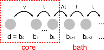
Figure 1: The semi-infinite tight-binding-chain is separated into two parts: The ’core’ includes the correlated site and L bath-sites. The ’bath’ consists of the remaining bath-sites. The two parts are coupled by a hopping-term which is proportional to the parameter $\Lambda$.

Our model is described by the grandcanonical partition function

$$\mathcal{Z}=\int\mathcal{D}\left[\bar{b},b\right]\ \exp\left[-S\left(\bar{b},b\right)\right]$$ (13)

with the action

$$S\left(\bar{b},b\right) = S_{core}\left(\bar{b}_{0},b_{0},\bar{b}_{1},b_{1},...,\bar{b}_{L},b_{L}\right)$$ (14)

$$+ S_{bath}\left(\bar{b}_{L+1},b_{L+1},\bar{b}_{L+2},b_{L+2},...\right)$$

$$+ S_{coupling}^{\Lambda}\left(\bar{b}_{L},b_{L},\bar{b}_{L+1},b_{L+1}\right)\,.$$

To make the notation more compact, we denote the dot-site $d$ as the 0th bath-site $b_{0}$. We define the scalar product

$$\left(\psi,\phi\right)=\int_{0}^{\beta}d\tau\sum_{\sigma}\psi_{\sigma}(\tau)\phi_{\sigma}(\tau).$$ (15)

$S_{core}$ and $S_{bath}$ are given by

$$S_{core}\left(\bar{b}_{0},b_{0},\bar{b}_{1},b_{1},...,\bar{b}_{L},b_{L}\right) = \left(\bar{b}_{0},(\partial_{\tau}+\epsilon_{d,\sigma})b_{0}\right)+U\ \int_{0}^{\beta}d\tau\ n_{\uparrow}\left(\tau\right)n_{\downarrow}\left(\tau\right)$$

$$-v\ \left[\left(\bar{b}_{0},b_{1}\right)+H.c.\right]+\sum_{j=1}^{L}\left(\bar{b}_{j},\partial_{\tau}b_{j}\right)-t\ \sum_{j=1}^{L-1}\left[\left(\bar{b}_{j},b_{j+1}\right)+H.c.\right]\,,$$

$$S_{bath}\left(\bar{b}_{L+1},b_{L+1},\bar{b}_{L+2},b_{L+2},...\right) = \sum_{j=L+1}^{\infty}\left(\bar{b}_{j},\partial_{\tau}b_{j}\right)-t\ \sum_{j=L+1}^{\infty}\left[\left(\bar{b}_{j},b_{j+1}\right)+H.c.\right],$$ (17)

where we introduced $n_{\sigma}(\tau)=\bar{b}_{0,\sigma}(\tau)b_{0,\sigma}(\tau)$. The coupling between the core and the bath is described by

$$S_{coupling}^{\Lambda}\left(\bar{b}_{L},b_{L},\bar{b}_{L+1},b_{L+1}\right)=-\Lambda t\ \left[\left(\bar{b}_{L},b_{L+1}\right)+H.c.\right].$$ (18)

We introduced the flow parameter $\Lambda$. The original model (1) corresponds to $\Lambda=1$ and for $\Lambda=0$ core and bath are decoupled. In the case $L=0$, $S_{core}$ is just given by the first line of Eq. (III.1) and one has to replace $\Lambda t$ by $\Lambda v$ in Eq. (18).

The generating functional for the connected Green’s functions of the core-problem is given by

$$\mathcal{W}_{core}\left(\bar{J},J\right)=\ln\left[\frac{1}{\mathcal{Z}_{core}}\int\mathcal{D}\left[\bar{c},c\right]\exp\left[-S_{core}\left(\bar{c},c\right)+\sum_{i=0}^{L}\left(\bar{J}_{i},c_{i}\right)+H.c.\right]\right]$$ (19)

with the core-fields $c=\left(b_{0},b_{1},b_{2},...,b_{L}\right)$. $\mathcal{Z}_{core}$ is the partition function of the core-problem given by

$$\mathcal{Z}_{core}=\int\mathcal{D}\left[\bar{c},c\right]\ \exp\left[-S_{core}\left(\bar{c},c\right)\right].$$ (20)

$\mathcal{W}_{core}$ can be expanded in the fields

$$\mathcal{W}_{core}\left(\bar{J},J\right)=\sum_{n=0}^{\infty}\frac{(-1)^{n}}{n!^{2}}\sum_{i_{1},...,i_{n}\atop i_{1}^{\prime},...,i_{n}^{\prime}}\int_{0}^{\beta}d\tau_{1}...\int_{0}^{\beta}d\tau_{n}\int_{0}^{\beta}d\tau_{1}^{\prime}...\int_{0}^{\beta}d\tau_{n}^{\prime} \mathcal{G}_{core}^{c,(n)}\left(i_{1},\tau_{1};...;i_{n},\tau_{n}|i_{1}^{\prime},\tau_{1}^{\prime};...;i_{n}^{\prime},\tau_{n}^{\prime}\right)$$ (21)

$$\times\bar{J}_{i_{1}}(\tau_{1})...\bar{J}_{i_{n}}(\tau_{n})J_{i_{n}^{\prime}}(\tau_{n}^{\prime})...J_{i_{1}^{\prime}}(\tau_{1}^{\prime})\,,$$

such that

$$\mathcal{G}_{core}^{c,(n)}\left(i_{1},\tau_{1};...;i_{n},\tau_{n}|i_{1}^{\prime},\tau_{1}^{\prime};...;i_{n}^{\prime},\tau_{n}^{\prime}\right)=\left.\frac{\delta^{2n}\mathcal{W}_{core}\left(\bar{J},J\right)}{\delta\bar{J}_{i_{1}}(\tau_{1})...\delta\bar{J}_{i_{n}}(\tau_{n})\delta J_{i_{n}^{\prime}}(\tau_{n}^{\prime})...\delta J_{i_{1}^{\prime}}(\tau_{1}^{\prime})}\right|_{J=\bar{J}=0}\,.$$ (22)

With the definition of the $(L+1)$-component field $\chi~{}=~{}t(0,0,...,b_{L+1})$ we can rewrite the action (14) as

$$S = S_{core}\left(\bar{c},c\right)-\sum_{i=0}^{L}\left(\bar{c_{i}},\Lambda\chi_{i}\right)-H.c.$$ (23)

$$+S_{bath}\left(\bar{b}_{L+1},b_{L+1},\bar{b}_{L+2},b_{L+2},...\right)\,.$$

Now we can formally integrate out the $c$-fields,

$$\int\mathcal{D}\left[\bar{c},c\right]\exp\left[-S_{core}\left(\bar{c},c\right)+\sum_{i=0}^{L}\left(\bar{c}_{i},\Lambda\chi_{i}\right)+H.c.\right]$$

$$=\mathcal{Z}_{core}\exp\left[\mathcal{W}_{core}\left(\Lambda\bar{\chi},\Lambda\chi\right)\right],$$

yielding an effective action for the bath

$$\mathcal{Z} = \int\mathcal{D}\left[\bar{c},c,\bar{b}_{L+1},b_{L+1},...\right]\exp\left[-S_{core}\left(\bar{c},c\right)+\sum_{i=0}^{L}\left(\bar{c}_{i},\Lambda\chi_{i}\right)+H.c.-S_{bath}\left(\bar{b}_{L+1},b_{L+1},\bar{b}_{L+2},b_{L+2},...\right)\right]$$

$$= \int\mathcal{D}\left[\bar{b}_{L+1},b_{L+1},\bar{b}_{L+2},b_{L+2},...\right]\exp\left[-S^{eff}_{bath}\left(\bar{b}_{L+1},b_{L+1},\bar{b}_{L+2},b_{L+2},...\right)\right].$$

When we expand $\mathcal{W}_{core}\left(\Lambda\bar{\chi},\Lambda\chi\right)$ in the $\bar{\chi},\chi$-fields the effective action has the following form

$$S^{eff}_{bath}\left(\bar{b}_{L+1},b_{L+1},\bar{b}_{L+2},b_{L+2},...\right)$$

$$= S_{bath}\left(\bar{b}_{L+1},b_{L+1},\bar{b}_{L+2},b_{L+2},...\right)-\mathcal{W}_{core}\left(\Lambda\bar{\chi},\Lambda\chi\right)$$

$$= S_{bath}\left(\bar{b}_{L+1},b_{L+1},\bar{b}_{L+2},b_{L+2},...\right)-\sum_{n=0}^{\infty}\frac{(-1)^{n}\Lambda^{2n}}{n!^{2}}\sum_{i_{1},...,i_{n}\atop i_{1}^{\prime},...,i_{n}^{\prime}}\int_{0}^{\beta}d\tau_{1}...\int_{0}^{\beta}d\tau_{n}\int_{0}^{\beta}d\tau_{1}^{\prime}...\int_{0}^{\beta}d\tau_{n}^{\prime}$$

$$\times\mathcal{G}^{c,(n)}_{core}\left(i_{1},\tau_{1};...;i_{n},\tau_{n}|i_{1}^{\prime},\tau_{1};,...;i_{n}^{\prime},\tau_{n}^{\prime}\right)\bar{\chi}_{i_{1}}(\tau_{1})...\bar{\chi}_{i_{n}}(\tau_{n})\chi_{i_{n}^{\prime}}(\tau_{n}^{\prime})...\chi_{i_{1}^{\prime}}(\tau_{1}^{\prime})\,.$$

In the following we neglect the term with $n=0$, which does not contain any fields. Furthermore, we truncate the sum over $n$ after $n=2$. This means we consider only the first and second order of the expansion and neglect all correlation-functions $\mathcal{G}^{c,(\geq 3)}_{core}$. When we transform the action to Matsubara frequencies we get

$$S^{eff}_{bath}\left(\bar{b}_{L+1},b_{L+1},\bar{b}_{L+2},b_{L+2},...\right)$$

$$= S_{bath}\left(\bar{b}_{L+1},b_{L+1},\bar{b}_{L+2},b_{L+2},...\right)+\frac{\Lambda^{2}}{\beta}\sum_{i\omega}\sum_{i_{1},i_{1}^{\prime}}\bar{\chi}_{i_{1}}(i\omega)\mathcal{G}^{c,(1)}_{core}\left(i\omega,i_{1},i_{1}^{\prime}\right)\chi_{i_{1}^{\prime}}(i\omega)$$

$$-\frac{\Lambda^{4}}{4\beta^{3}}\sum_{i\omega_{1},i\omega_{2},\atop i\omega_{1}^{\prime},i\omega_{2}^{\prime}}\sum_{i_{1},i_{2},\atop i_{1}^{\prime},i_{2}^{\prime}}\bar{\chi}_{i_{1}}(i\omega_{1})\bar{\chi}_{i_{2}}(i\omega_{2})\mathcal{G}^{c,(2)}_{core}\left(i\omega_{1},i_{1};i\omega_{2},i_{2}|i\omega_{1}^{\prime},i_{1}^{\prime};i\omega_{2}^{\prime},i_{2}^{\prime}\right)\chi_{i_{1}^{\prime}}(i\omega_{1}^{\prime})\chi_{i_{2}^{\prime}}(i\omega_{2}^{\prime})\delta_{\omega_{1}+\omega_{2},\omega_{1}^{\prime}+\omega_{2}^{\prime}}$$

$$= S_{bath}\left(\bar{b}_{L+1},b_{L+1},\bar{b}_{L+2},b_{L+2},...\right)+\frac{(\Lambda t)^{2}}{\beta}\sum_{i\omega}\sum_{\sigma}\bar{b}_{L+1,\sigma}(i\omega)\mathcal{G}^{c,(1)}_{core,\sigma}\left(i\omega,b_{L},b_{L}\right)b_{L+1,\sigma}(i\omega)$$

$$-\frac{(\Lambda t)^{4}}{4\beta^{3}}\sum_{i\omega_{1},i\omega_{2},\atop i\omega_{1}^{\prime},i\omega_{2}^{\prime}}\sum_{\sigma_{1},\sigma_{2},\atop\sigma_{1}^{\prime},\sigma_{2}^{\prime}}\bar{b}_{L+1,\sigma_{1}}(i\omega_{1})\bar{b}_{L+1,\sigma_{2}}(i\omega_{2})\mathcal{G}^{c,(2)}_{core}\left(i\omega_{1},b_{L},\sigma_{1};i\omega_{2},b_{L},\sigma_{2}|i\omega_{1}^{\prime},b_{L},\sigma_{1}^{\prime};i\omega_{2}^{\prime},b_{L},\sigma_{2}^{\prime}\right)$$

$$\times b_{L+1,\sigma_{1}^{\prime}}(i\omega_{1}^{\prime})b_{L+1,\sigma_{2}^{\prime}}(i\omega_{2}^{\prime})\delta_{\omega_{1}+\omega_{2},\omega_{1}^{\prime}+\omega_{2}^{\prime}}\delta_{\sigma_{1}+\sigma_{2},\sigma_{1}^{\prime}+\sigma_{2}^{\prime}}\,.$$

In the effective-bath theory there is a local interaction on bath site $L+1$. The other bath sites ($L+2$,$L+3$,…) remain noninteracting and can be integrated out. This leads to the local effective action

$$S^{eff}_{bath}\left(\bar{b}_{L+1},b_{L+1}\right) = -\frac{1}{\beta}\sum_{i\omega}\sum_{\sigma}\bar{b}_{L+1,\sigma}(i\omega)\left(i\omega-(\Lambda t)^{2}\mathcal{G}^{c,(1)}_{core,\sigma}\left(i\omega,b_{L},b_{L}\right)-t^{2}g_{b}\left(i\omega,b_{1},b_{1}\right)\right)b_{L+1,\sigma,i\omega}$$ (24)

$$-\frac{(\Lambda t)^{4}}{4\beta^{3}}\sum_{i\omega_{1},i\omega_{2},\atop i\omega_{1}^{\prime},i\omega_{2}^{\prime}}\sum_{\sigma_{1},\sigma_{2},\atop\sigma_{1}^{\prime},\sigma_{2}^{\prime}}\bar{b}_{L+1,\sigma_{1}}(i\omega_{1})\bar{b}_{L+1,\sigma_{2}}(i\omega_{2})\mathcal{G}^{c,(2)}_{core}\left(i\omega_{1},b_{L},\sigma_{1};i\omega_{2},b_{L},\sigma_{2}|i\omega_{1}^{\prime},b_{L},\sigma_{1}^{\prime};i\omega_{2}^{\prime},b_{L},\sigma_{2}^{\prime}\right)$$

$$b_{L+1,\sigma_{1}^{\prime}}(i\omega_{1}^{\prime})b_{L+1,\sigma_{2}^{\prime}}(i\omega_{2}^{\prime})\delta_{\omega_{1}+\omega_{2},\omega_{1}^{\prime}+\omega_{2}^{\prime}}\delta_{\sigma_{1}+\sigma_{2},\sigma_{1}^{\prime}+\sigma_{2}^{\prime}}\,.$$

The local correlation functions of the core, $\mathcal{G}^{c,(1)}_{core}$ and $\mathcal{G}^{c,(2)}_{core}$ can be calculated from the Lehmann representation, which is given in appendix C. Note that for $\Lambda=0$, the bath theory is noninteracting. The exact solution of this serves as an initial condition for the fRG flow in $\Lambda$.

III.2 Relation to the Dot self-energy

In the effective theory (24) the bath site $L+1$ is now interacting with a frequency dependent term, while in the original theory (14) it was noninteracting. The self-energy and all higher irreducible vertex-functions are local on the dot-site by construction . Nevertheless the local Green’s function of the coupled problem on bathsite $L+1$ is nontrivial and depends on the dot self-energy, as can be seen in (68) or (69). This Green’s function can also be derived in the setup of the effective theory and one can use the identity $\mathcal{G}_{\sigma}\left(i\omega_{n},b_{L+1},b_{L+1}\right)=\mathcal{G}^{eff}_{\sigma}\left(i\omega_{n},b_{L+1},b_{L+1}\right)$ with

$$\mathcal{G}^{eff}_{\sigma}\left(i\omega_{n},b_{L+1},b_{L+1}\right)=$$ (25)

$$\left[i\omega-(\Lambda t)^{2}\mathcal{G}^{c,(1)}_{core,\sigma}\left(i\omega,b_{L},b_{L}\right)-t^{2}g_{b}\left(i\omega\right)-\Sigma_{b,\sigma}(i\omega)\right]^{-1}$$

to get a relation between the dot self-energy and the effective self-energy $\Sigma_{b}$ on bath site $L+1$. These relations depend on $L$ and for $L=0,1,2,3$ we get the relations given in Eq. (70)-(73) in appendix B.

IV Functional RG flow equations

The effective action in Eq. (24) reduces to a noninteracting model for $\Lambda=0$, because the interaction term is proportional to $\Lambda^{4}$. This represents a simple starting point for a fRG flow in $\Lambda$. In order to use the fRG formalism for one-particle irreducible (1PI) vertices Wetterich (1993); Salmhofer and Honerkamp (2001); Metzner et al. (2012), the flow parameter $\Lambda$ should only occur in the quadratic part of the action. This can be achieved for any $\Lambda\not=0$ by rescaling the fields $b_{L+1}\to b_{L+1}/\Lambda$ and $\bar{b}_{L+1}\to\bar{b}_{L+1}/\Lambda$. This leads to the quadratic part of the effective action,

$$S^{eff,0}_{bath}\left(\bar{b}_{L+1},b_{L+1}\right) = -\frac{1}{\beta}\sum_{i\omega}\sum_{\sigma}\bar{b}_{L+1,\sigma}(i\omega)Q^{\Lambda}_{\sigma}\left(i\omega\right)b_{L+1,\sigma,i\omega}.$$

with

$$Q^{\Lambda}_{\sigma}\left(i\omega\right)=\frac{i\omega}{\Lambda^{2}}-t^{2}\mathcal{G}^{c,(1)}_{core,\sigma}\left(i\omega,b_{L},b_{L}\right)-\frac{t^{2}}{\Lambda^{2}}g_{b}\left(b_{1},b_{1},i\omega\right)$$ (26)

and quartic part which does not depend on $\Lambda$ anymore. Note that the rescaling changes correlation functions of different order in the fields differently, but in the end we will study the case $\Lambda=1$. The one-particle-irreducible-(1PI)-vertex-functions on scale $\Lambda$ can be calculated by an infinite set of exact flow-equations. Wetterich (1993); Salmhofer and Honerkamp (2001); Metzner et al. (2012) If we neglect the flow of the three-particle-vertex and of all higher vertex functions we get a closed set of equations for the self-energy $\Sigma_{b}^{\Lambda}$ and the two-particle vertex-function $\Gamma_{b}^{\Lambda}$,

$$\frac{d}{d\Lambda}\Sigma_{b}^{\Lambda}(k^{\prime};k)=-\textrm{Tr}\left[S^{\Lambda}\Gamma_{b}^{\Lambda}(k^{\prime},.;k,.)\right]$$ (27)

$$\frac{d}{d\Lambda}\Gamma_{b}^{\Lambda}(k_{1}^{\prime},k_{2}^{\prime};k_{1},k_{2})=\textrm{Tr}\left[S^{\Lambda}\Gamma_{b}^{\Lambda}(k_{1}^{\prime},k_{2}^{\prime},.;k_{1},k_{2},.)\right]$$

$$-\textrm{Tr}\left[S^{\Lambda}\Gamma_{b}^{\Lambda}(.,.;k_{1},k_{2})[\mathcal{G}^{\Lambda}]^{T}\Gamma_{b}^{\Lambda}(k_{1}^{\prime},k_{2}^{\prime};.,.)\right]$$

$$-\textrm{Tr}\left[S^{\Lambda}\Gamma_{b}^{\Lambda}(k_{1}^{\prime},.;k_{1},.)\mathcal{G}^{\Lambda}\Gamma_{b}^{\Lambda}(k_{2}^{\prime},.;k_{2},.)\right]$$

$$-[k_{1}^{\prime}\leftrightarrow k_{2}^{\prime}]-[k_{1}\leftrightarrow k_{2}]+[k_{1}^{\prime}\leftrightarrow k_{2}^{\prime},k_{1}\leftrightarrow k_{2}],$$ (28)

in which $\mathcal{G}^{\Lambda}$ is the full propagator and $S^{\Lambda}$ is the so called single-scale propagator defined by

$$S^{\Lambda}=\mathcal{G}^{\Lambda}\frac{d}{d\Lambda}\left[Q^{\Lambda}\right]\mathcal{G}^{\Lambda}.$$ (29)

The $k_{i}^{(^{\prime})}$ denote one-particle-quantum-numbers (in our case Matsubara-freqency, spin and site-index) and the trace is defined with respect to these quantum numbers. In the case $B=0$, the flow-equations (27) and (IV) can be further simplified by using the spin-rotation-invariance of the effective action (IV), which is described in appendix D.

By integrating the flow-equations from $\Lambda=0$ to $\Lambda=1$ we can derive the self-energy of the effective bath theory. Using the relations (70) - (73) we obtain the dot self-energy $\Sigma_{d}\left(i\omega\right)$.

In the simplest approximation one neglects the flow of the two-particle-vertex and integrates equation (27) with $\Gamma_{b}^{\Lambda}=\Gamma_{b}^{\Lambda=0}$ (in the following called ’approximation 1’), where $\Gamma_{b}^{\Lambda=0}$ is given by Eqs. (D) and (85). If one integrates the full set of Eqs. (27) and (IV) (called ’approximation 2’) the numerical effort scales with the third power of the number of Matsubara-frequencies.

Motivated by the fullfillment of Ward-identities in the RG-flow, the following replacement in the flow-equation for the vertex-function was proposed,Katanin (2004)

$$S^{\Lambda}\rightarrow-\frac{d\mathcal{G}^{\Lambda}}{d\Lambda}=S^{\Lambda}-\mathcal{G}^{\Lambda}\frac{d\Sigma_{b}^{\Lambda}}{d\Lambda}\mathcal{G}^{\Lambda}\,.$$ (30)

This replacement is used in all following calculations.

Instead of doing the fRG-flow in the effective bath-theory (IV) one can also derive flow-equations for the dot self-energy (70)- (73) and the two-particle-(1PI)-vertex on the dot-site with the core-(1PI)-vertex-functions as initial condition. For $L>0$ these flow-equations have a more complicated structure than in our case and the calculations are easier in the setup of the effective bath-theory. For $L=0$ and approximation 1 we compared both schemes. It turned out that neglecting the flow of the 2-particle-vertex of the effective bath-theory leads to better results than doing an analogous approximation for the 2-particle-vertex on the dot.

V Numerical results

In the following we present our results for different sizes of the core ($L=0,1$ and $L=3$). The data shown here was produced by integrating Eqs. (27, IV) numerically from $\Lambda=0$ to $\Lambda=1$, using typically 100 to 200 Matsubara frequencies at temperatures varying between $\beta=20/\Delta_{0}$ and $\beta=50/\Delta_{0}$. We set $\Delta_{0}=1$ giving the energy scale and in most cases consider particle-hole symmetry, $\epsilon_{d}=-U/2$. The results are compared with other fRG approaches and benchmark NRG calculations. The latter are carried out with the same semi-elliptic density of states. We focus on quantities that can directly be calculated from the data on the imaginary frequency-axis. One of these quantities is the effective mass $m^{*}$ given by

$$m^{*}=z^{-1}=1-\left.\frac{d\text{Im}\Sigma_{d}\left(i\omega\right)}{d\omega}\right|_{\omega=0^{+}}.$$ (31)

In the Kondo-regime the quasiparticle weight $z$ determines the width of the Kondo-resonance and is expected to scale exponentially with the interaction strength. We furthermore calculate the linear conductance of the dot $G=\sum_{\sigma}G_{\sigma}$ given by (in the following we set $\hbar=e^{2}=1$)

$$G_{\sigma} = \frac{1}{2}\pi v^{2}\int d\omega A_{d,\sigma}\left(\omega\right)\rho_{b}\left(\omega\right)\left(-\frac{\partial n_{F}\left(\omega\right)}{\partial\omega}\right)$$ (32)

$$\simeq \frac{1}{2}\Delta_{0}\int d\omega A_{d,\sigma}\left(\omega\right)\left(-\frac{\partial n_{F}\left(\omega\right)}{\partial\omega}\right)\,.$$

In the second line we used that the derivative of the Fermi-function is sharply peaked at low temperature at $\omega=0$ so that the $\omega$-dependence of $\rho_{b}(\omega)$ can be neglected. Of course the conductance is derived by an integral over the real frequency axis and at first sight one has also to perform an analytic continuation. To circumvent this, we follow an approach, proposed in Ref. Karrasch et al., 2010b, that does not require an analytic continuation. In this approach $G$ follows from the formula

$$G_{\sigma}\simeq\Delta_{0}T\sum_{\alpha>0}R_{\alpha}\text{Im}\frac{d\mathcal{G}_{\sigma}(i\tilde{\omega}_{\alpha})}{d\tilde{\omega}_{\alpha}},$$ (33)

where the imaginary frequencies $i\tilde{\omega}_{\alpha}$ and the weights $R_{\alpha}$ are defined in Ref. Karrasch et al., 2010b. The frequencies $i\tilde{\omega}_{\alpha}$ differ from the original Matsubara-frequencies and we determine $\frac{d\mathcal{G}_{\sigma}(i\tilde{\omega}_{\alpha})}{d\tilde{\omega}_{\alpha}}$ from a Pade-approximation.

We have also done the analytic continuation $\mathcal{G}\left(i\omega_{n},d,d\right)\rightarrow\mathcal{G}\left(\omega+i0^{+},d,d\right)$ to the real frequency axis using a Pade-algorithm described in Ref. Vidberg and Serene, 1977. As the analytical continuation of numerical data is mathematically an ill-defined problem we did not obtain numerically stable and meaningful results for all parameter sets.

V.1 The case $L=0$

For $L=0$ the ’core’ is given by an isolated dot site. In this case the core-correlation-functions can be calculated analytically Hafermann et al. (2009) and one can also derive analytical results in the setup of the effective bath-theory. Joerg (2010)

The initial self-energy at $\Lambda=0$ for $\epsilon_{d}=-U/2$ is given by

$$\Sigma_{d}\left(i\omega\right)=\frac{U}{2}+\frac{U^{2}}{4i\omega},$$ (34)

which is the atomic limit result. $\Sigma_{d}\left(i\omega\right)$ diverges at $i\omega=0$. In Fig. 2 (upper panel) we show the $i\omega$-dependenc of the self-energy at the end of the flow for $\Lambda=1$ on the dot for $U=10\Delta_{0}$, $\beta=30/\Delta_{0}$ and for the particle-hole symmetric case, $V_{g}=0$, computed with the described fRG-flow in both approximations 1 and 2. In the calculation we included 200 Matsubara-frequencies. The divergence of the self-energy at $i\omega=0$ has disappeared, but there is still a discontinuity, which is not cured by the flow. This shows the flow equations are not able to restore the expected local Fermi liquid properties of the SIAM, if we start with the atomic solution. The height of the unphysical discontinuity becomes however smaller in approximation 2 compared to approximation 1.

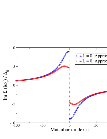
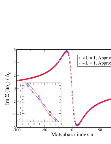
Figure 2: (color online) Comparison of approximations 1 and 2 to the Matsubara-self-energy for $U=10\Delta_{0}$, $\beta=30/\Delta_{0}$ and $L=0,1$. For $L=0$ one gets a discontinuity of $\text{Im}\Sigma(i\omega_{n})$ between positive and negative Matsubara-frequencies, which is reduced if one increases the level of approximation. For $L=1$, approximation 1 the self-energy is continuous for small frequencies. As shown in the inset one obtains a small step between positive and negative frequencies in approximation 2.

In the spectral density derived from a Pade-approximation to our numerical data at half filling (not shown) two slightly broadened atomic limit peaks at $\pm U/2$, but no central Kondo-resonance at small frequencies appears. Hence the $L=0$ approximation fails to describe the screening of the local spin-1/2-moment by the conduction-electrons. This screening and singlet formation should develop when $\Lambda$ is switched on, while at $\Lambda=0$ the local moment is unscreened. We assume that this strong mismatch is the reason for the non-occurence of the Kondo-resonance in this approximation.

Our results are consistent with the findings in Ref. Hafermann et al., 2009, where a superperturbation approach to the Anderson model is developed. In this approach a finite local cluster containing the correlated dot-site is solved exactly. The correlation-functions of this cluster then serve as input for an effective theory of dual-fermion-fields. Like in our setup, no Kondo-resonance is found when the cluster contains only the correlated bath-site.

V.2 The cases $L=1,2$ and $3$

In the case $L=1$ the isolated core consists of an interacting site coupled by a hopping-term $v$ to a noninteracting bath-site. This model is still analytically solvable. The ground-state at half-filling is a spin-singlet-state. For $\epsilon_{d}=-U/2$ and in the limit $v\ll U$ and this state is given by

$$|S=0\rangle=\frac{4v}{U}\left(\ket{\uparrow\downarrow,e}+\ket{e,\uparrow\downarrow}\right)-\left(1-\frac{8v^{2}}{U^{2}}\right)\left(\ket{\uparrow,\downarrow}-\ket{\downarrow,\uparrow}\right)$$ (35)

with energy $\frac{1}{4}\left(-U-\sqrt{U^{2}+64v^{2}}\right)\overset{v\ll U}{\approx}-\frac{U}{2}-\frac{8v^{2}}{U}$. The first entry in $|.,.\rangle$ is the correlated site, the second the additional uncorrelated core site. $e$ stands for an empty site. Now, in contrast to the case $L=0$, the local-moment on the dot is already in a singlet state for $\Lambda=0$. This is a much better starting point to describe features of the Kondo effect. As can be seen in Fig. 2 the self-energy at the end of the flow for $L=1$ is continuous at $i\omega=0$. For $L=2$ the isolated core self-energy has a similar shape as in the $L=0$-case and for $\Lambda=1$ we get a finite step between positive and negative Matsubara-frequencies. In its groundstate the core carries again a finite $s=1/2$-moment, doublet ground state, in this case which does not become screened when we switch on the coupling to the bath in the fRG-flow. This shows once more the importance of choosing a core with spin-singlet groundstate for an at least qualitatively correct description of Kondo screening in this setup. The next larger core size with a singlet groundstate contains $L=3$ bath sites. Numerically the calculation of the two-particle vertex function is limited due to the exponential growth of the core-Hilbert-space. We just used approximation 1 in the $L=3$ case, because here we only need to calculate the vertex for two instead of three independent frequencies.

Let us now discuss the numerical results in more detail. The spectrum of the isolated two-site core with $L=1$ consists of four delta-peaks. Two of them are located at $\epsilon_{1,2}=\pm\frac{1}{4}\left(\sqrt{U^{2}+64v^{2}}+\sqrt{U^{2}+16v^{2}}\right)\overset{v\ll U}{\approx}\pm\left(\frac{U}{2}+\frac{10v^{2}}{U}\right)$, which belong to excitations from the ground-state (35) to the one-particle-state $\frac{2v}{U}\ket{\sigma,e}+\left(1-\frac{2v^{2}}{U^{2}}\right)\ket{e,\sigma}\quad(v\ll U)$ and its corresponding three-particle-state, which is connected by a particle-hole-transformation. In the limit $v\rightarrow 0$ they are equal to the atomic $\pm U/2$-excitations of the L=0-core. When we switch on the coupling to the bath in the fRG-flow, they evolve into hybridization broadened peaks. The other two peaks in the spectrum of the L=1-core lie at $\epsilon_{3,4}=\pm\frac{1}{4}\left(\sqrt{U^{2}+64v^{2}}-\sqrt{U^{2}+16v^{2}}\right)\overset{v\ll U}{\approx}\pm\frac{6v^{2}}{U}$. They belong to excitations from the ground-state to the one-particle-state $\frac{2v}{U}\ket{\sigma,e}+\left(1-\frac{2v^{2}}{U^{2}}\right)\ket{e,\sigma}\quad(v\ll U)$ and its corresponding three particle-state. Note, that due to these excitations, there is a finite spectral weight near zero-energy already for $\Lambda=0$ that can evolve into a central Kondo resonance.

It turns out that already in the most simple approximation 1 we get a quasiparticle resonance at $\omega=0$. The change of the spectrum for different values of $\Lambda$ is shown in Fig. 3 for $U=6\Delta_{0}$. The peaks $\epsilon_{1,2}$ become slightly broadened, but their positions does not change significantly. In the end of the flow (for $\Lambda=1$) their maxima are not located at $\pm U/2=\pm 3\Delta_{0}$, the position usually expected in the wide band limit with a purely imaginary hybridization function $\Delta(\omega)$. However, in the present case where the bandwidth is less than $U$ the hybridization function $\Delta(\omega)$ has a finite real part which renormalizes this position. The position of the peaks, $\pm 3.9\Delta_{0}$ turns out to be comparable with what is found in NRG calculations. The small broadening of these high-energy peaks is related to the fact that they lie outside the bandwidth $(-2\Delta_{0},2\Delta_{0})$ of the bath, such that the width is purely due to self-energy effects. During the flow, already for small values of $\Lambda$, the low-energy peaks $\epsilon_{3,4}$ become broadened and a central resonance at $\omega=0$ with $A_{d}(\omega=0)=\frac{1}{\pi\Delta_{0}}$ emerges. Note that at the end of the flow, for $\Lambda=1$, there are still remnants of the peaks $\epsilon_{3,4}$, which is interpreted as an artefact of the approximation. The same artefacts are obtained for $L=3$.

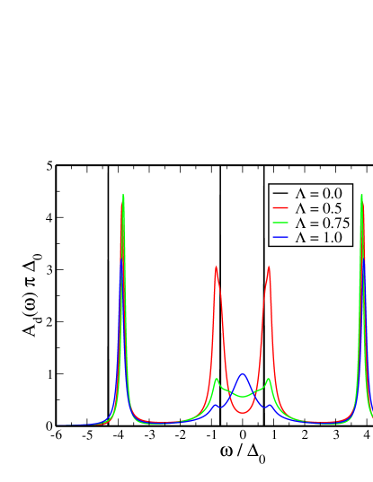
Figure 3: (color online) $L=1$ dot-spectra for several values of $\Lambda$ at half filling and $U=6\Delta_{0}$ and $\beta=50/\Delta_{0}$, obtained from a Pade-approximation to our numerical data on the imaginary frequency axis. The atomic limit peaks become slightly broadened and their position changes from 4.2$\Delta_{0}$ to 3.9$\Delta_{0}$. At small frequencies a central resonance with height $A_{d}(\omega=0)=1/\pi\Delta_{0}$ is emerging during the fRG flow from $\Lambda=0$ to $\Lambda=1$.

In Fig. 2 the self-energy calculated in approximation 1 and 2 is shown. In approximation 1 the self-energy is continuous for small frequencies and the derivative $\left.\frac{d\text{Im}\Sigma_{d}\left(i\omega\right)}{d\omega}\right|_{\omega=0^{+}}$ is negative, which leads to a reduced width $z\Delta_{0}$ of the resonance at small frequencies. As shown in the inset of Fig. 2 we obtain a small step between positive and negative Matsubara frequencies in approximation 2. This step leads to a slight broadening of the central resonance, which decreases with decreasing temperature. Therefore it can be understood as a physically sensible finite-temperature effect.

V.3 Results for the effectve mass in comparison

In Fig. 5 we show the effective mass for $L=1$, approximation 1 and 2 and $L=3$, approximation 1 in comparison with NRG data as function of the interaction strength $U$. The NRG-data is calculated at $T=0$ for a semi-elliptic bath-density of states. While the qualitative behaviour is similar, the effective mass from the fRG-calculations is systematically too small compared with the NRG data and we can not reproduce the exponential Kondo-scale quantitatively. For interaction-strengths $U\sim 8-9\Delta_{0}$ the Kondo-scale $T_{K}=W\sqrt{\frac{2\Delta_{0}}{\pi U}}\exp\left(-\frac{\pi U}{8\Delta_{0}}\right)$ becomes comparable with the temperature $T_{K}\approx\frac{1}{\beta}$, which we expect to be part of the reason for the deviations from the NRG result at large values of $U$. Note the slight increase of $m^{*}$ with decreasing temperature in Fig. 5. Our results for the effective mass fall in the range of other fermionic fRG-approaches to the Anderson-model Karrasch et al. (2008); Jakobs et al. (2010) (cf. Fig. 5), that are calculated for a bath in the wide-band-limit. A direct comparison of the data needs to take into account the fact that as can be seen from the NRG-data in Fig. 5 the effective mass for a semielliptic density of states with finite bandwidth is in general larger than for a bath in the wide-band-limit. The failure in reproducing the exponential Kondo-scale in the effective mass precisely is however common to all finite-frequency fRG-approaches to the Anderson model. Note, that all fRG-approaches truncate the hierarchy of flow-equations after the four-point level. Hence, we expect that this approximation is the reason for this deviation.

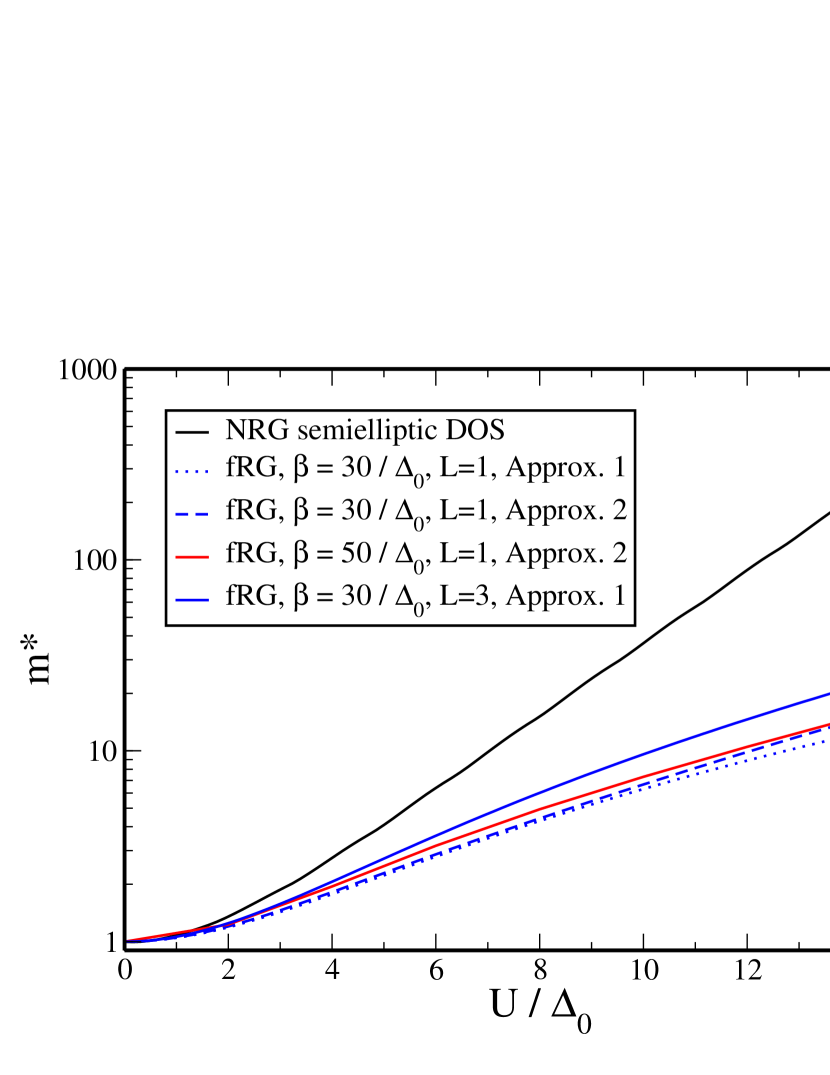
Figure 4: (color online) Effective mass ($\beta=30,50/\Delta_{0}$) for L=1, approximation 1 and 2 and for L=3, approximation 1 in comparison with NRG-data. The NRG-data are calculated for a bath with semi-elliptic density of states.

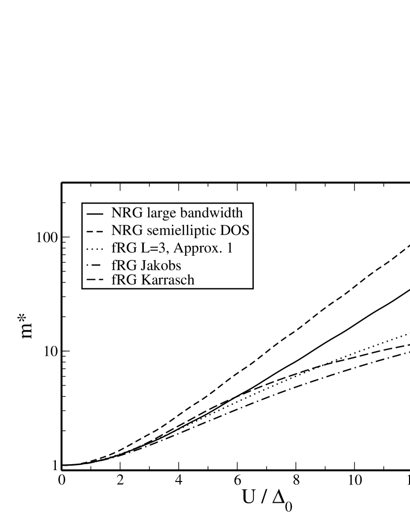
Figure 5: Effective mass ($\beta=30/\Delta_{0}$) for L=3, approximation 1 in comparison with fRG data from Ref. Jakobs et al., 2010 and approximation 1 in Ref. Karrasch et al., 2008. As reference data we show NRG-calculations for a semielliptic density of states and in the wide-band-limit.

V.4 Results for the conductance

Furthermore we calculated the linear conductance $G$ from Eq. (33). In Fig. 7 we show $G$ as function of the gate-voltage $V_{g}$ for several temperatures and $U=8\Delta_{0}$. At low temperatures $\beta=50/\Delta_{0}$ we get a plateau in the conductance for gatevoltages between $-\frac{U}{2}$ and $\frac{U}{2}$, which is due to the pinning of spectral weight at the Fermi energy. The plateau-value is given by the unitary limit $2G_{0}=2e^{2}/h$. For higher temperatures the conductance at $V_{g}=0$ decreases quadratically with the temperature.

In Fig.  7 the linear conductance derived in the two approximation schemes 1 and 2 is shown. In approximation 2 the linear conductance for small gate-voltages is reduced in comparison with approximation 1. We understand this again as a finite-temperature effect. In approximation 2, the Kondo peak gets narrower, i.e. the effective Kondo scale comes out smaller. Hence, in this approximation the actual temperature $\beta^{-1}$ is closer to $T_{K}$ as in approximation 1 and the conductivity shows a stronger finite-temperature suppression.

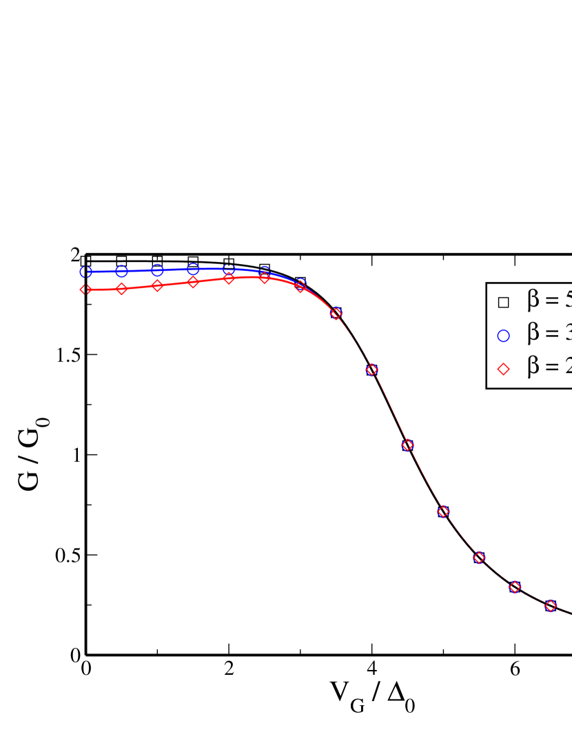
Figure 6: (color online) Comparison of the linear conductance for $U=8\Delta_{0}$ and $\beta=20,30,50/\Delta_{0}$, calculated in approximation 1. The value $G(V_{G}=0)$ decreases quadratically with increasing temperature.

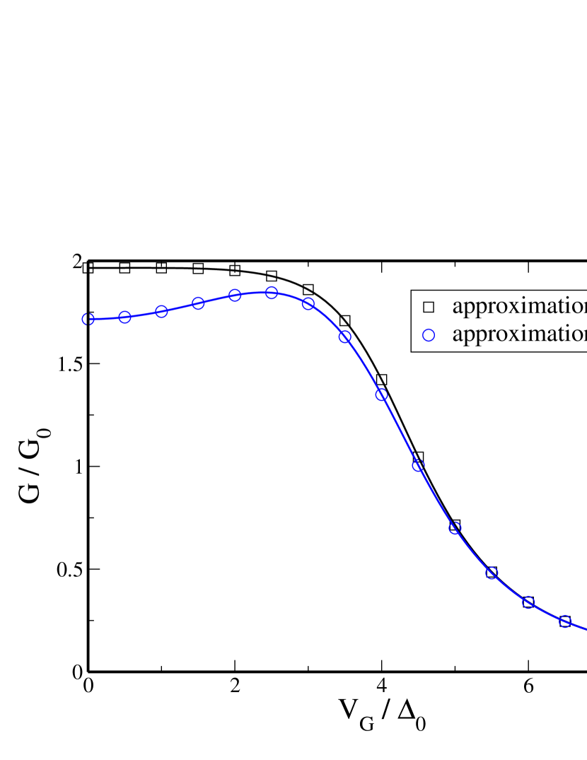
Figure 7: (color online) Comparison of approximation 1 and 2 to the linear conductance for $U=8\Delta_{0}$, $\beta=50/\Delta_{0}$.

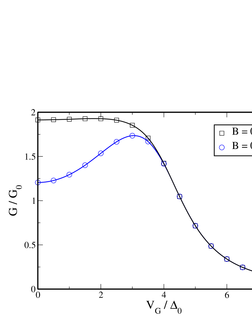
Figure 8: (color online) Linear conductance for $U=8\Delta_{0}$, $\beta=30/\Delta_{0}$ and several values of the magneticfield, calculated in approximation 1.

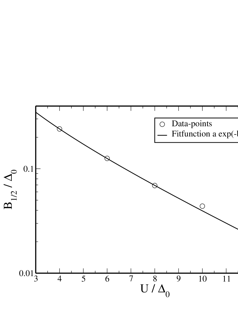
Figure 9: (color online) $B_{1/2}$ as function of $U$, $\beta=30/\Delta_{0}$, approximation 1, together with an exponential fit curve.

Fig.  (9) shows the suppression of the gate-voltage at $V_{G}=0$ due to a finite magnetic field. As shown in Ref. Karrasch et al., 2006 one can extract the Kondo-scale from this supression within a frequency-independent fRG-scheme with frequency-cutoff. Therefore one defines the Kondo scale $T_{K}$ as equal to the magnetic field $B_{1/2}$ that is required to suppress the gate voltage $G(V_{G}=0)$ to $G_{0}=e^{2}/h$, which is one half of the unitary limit. In Fig. (9) we show $B_{1/2}$ as function of $U$. As shown the data for small $U$ can be fitted to an exponential curve of the form $a\exp\left(-b\,U/\Delta_{0}\right)$. This behaviour is expected in the Kondo-regime. Here we find it already for these intermediate values of $U$. For larger $U$ there are systematic deviations from exponential behaviour. These deviations begin at $U\sim 8-9\Delta_{0}$, where the Kondo scale according to this association becomes comparable to the temperature, $T_{K}\approx\frac{1}{\beta}=\frac{\Delta_{0}}{30}$. From our fit we get $b\approx 0.32$, in good agreement with the exact value $b=\pi/8\approx 0.39$. Hewson (1993)

V.5 Results for the magnetic suseptibility and Wilson ratio

We also calculated the static magnetic susceptibility which is defined by

$$\chi_{s}=\frac{d\left(\langle n_{\uparrow}\rangle-\langle n_{\downarrow}\rangle\right)}{dB}\bigg{|}_{B=0}.$$ (36)

Here $\langle n_{\sigma}\rangle$ is the average occupation of electrons with spin $\sigma$, which is calculated by

$$\langle n_{\sigma}\rangle=\frac{1}{2}+2T\sum_{\alpha>0}R_{\alpha}\text{Re}\mathcal{G}_{\sigma}(i\tilde{\omega}_{\alpha})$$ (37)

with the same $R_{\alpha}$ and $\tilde{\omega}_{\alpha}$ as in Eq. 33.

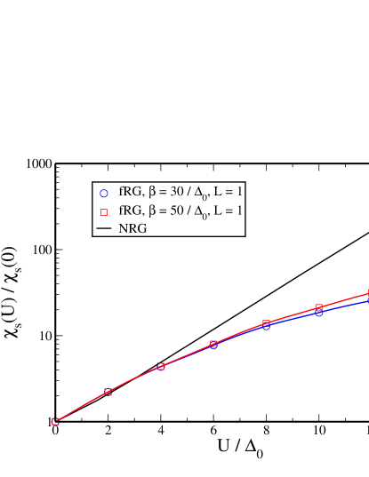
Figure 10: (color online) Magnetic susceptibility as function of $U$, $\beta=30/\Delta_{0},50/\Delta_{0}$, approximation 1 in comparison with NRG-data.

In Fig. 10 we show the spin-susceptibility in comparison with NRG-data. For large values of $U$ the spin-susceptibility is expected to be inversely proportional to the Kondo temperature $\chi_{s}\sim 1/T_{K}$. Therefore one expects an exponential dependence on the interaction strength. While the susceptibility definitely rises with increasing $U$, the exponential behaviour is not found in our fRG-approach. A part of this deviation might again be a thermal effect, as for $U\gtrsim 8-9\Delta_{0}$ the Kondo temperature falls below $\beta^{-1}$ where the calculation takes place.

In Fig. 11 we show the Wilson ratio which is calculated as $R=\frac{2\chi_{s}}{\chi_{s}+\chi_{c}}$ with the charge-susceptibility $\chi_{c}=\lim_{\mu\rightarrow 0}\sum_{\sigma}\frac{d\langle n_{\sigma}\rangle}{d\mu}$. With the relation $\frac{1}{m^{*}}=\frac{4}{\pi\Delta_{0}(\chi_{s}+\chi_{c})}$, which holds in the Anderson impurity model Hewson (1993); Kopietz et al. we get $R=\frac{\Delta_{0}\pi\chi_{s}}{2m^{*}}$. Therefore we can calculate $R$ from our data of the effective mass and the spin-susceptibility. $R=2$ corresponds to the Kondo regime, where charge fluctations are completely suppressed and the charge-susceptibility vanishes. As seen in Fig. 11, for $U\gtrsim 8\Delta_{0}$ the fRG-data come out very close to $R=2$ even though $\chi_{s}$ is too small in the fRG. This points to advantageous cancellations of errors for this ratio in the fRG. Indeed $m^{*}$ comes out too small as well. The slight decrease of $R$ for $U>9\Delta_{0}$ might be again due effects of finite temperature.

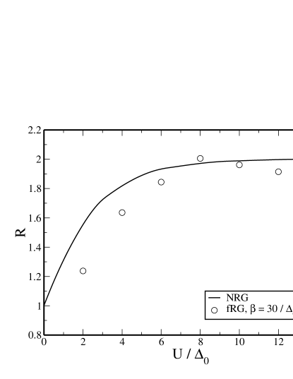
Figure 11: Wilson ratio R as function of $U$, $\beta=30/\Delta_{0}$, approximation 1 in comparison with NRG-data.

VI Conclusion

We have presented an alternative renormalization group approach to the single-impurity Anderson model. The starting point is the exact result for self-energy and four-point vertex of a small subsystem (’core’) containing the correlated impurity site. Then we track the evolution of these two functions when the coupling to the bath is switched on slowly. This way, the solution of the small isolated cluster is implemented exactly, and the flow generates changes of infinite order in the hybridization with the bath. The main approximation is the truncation of the flow equations after the four-point vertex. In the present case this means that the change of the higher-order vertices (six-point, eight-point, etc.) upon coupling to the bath is not allowed to influence the lower order vertices, i.e. the two-particle interaction and the self-energy. Yet, the idea that led us take this avenue was that starting with the exact two-point and four-point vertex of the small core contains enough strong correlation physics in order to give a physically reasonable results. The local interacting physics, such as the atomic scales are well represented in our approach. However, the Kondo effect requires to describe the subtle interplay with a continuum of states including many energy scales and our approach captures this only qualitatively, but not quantitatively. We expect this to be less of a problem in a self-consistent approach, such as DMFT, where for stronger coupling the Kondo resonance does not survive.

Indeed, the numerical results for clusters with an odd number of auxiliary sites ($L=1$ and $L=3$) show that the flow equations produce qualitatively correct results, whereas for even numbers the Fermi liquid behavior is not recovered. The dependence of the width of the Kondo peak with increasing $U$ is quantitatively different from NRG results, i.e. the correct exponential dependence is not reproduced. For larger $U$ the Kondo scale gets smaller than the nonzero temperatures for which the fRG scheme is feasible. So no clear statement can be made regarding the large-$U$ behavior. However, in the interesting intermediate coupling regime, the deviations may be tolerable. In this sense embedding this new impurity solver in a different contexts to describe itinerant and strongly coupled physics qualitatively correctly (see discussion below) seems a viable possibility.

In comparison with other finite-frequency functional RG techniques, e.g. those that are perturbative in $U$, our data end up in the same range, as shown in Fig. 5. As the ground state for weak and strong coupling remains the same, it is not entirely surprising that approaches starting at the opposite ends lead to qualitatively similar answers. The quantitative agreement could however be interpreted further, as a measure of what is missed by the truncation after the four-point vertex that is common to both lines of approach. Note, that in a recent paper Streib et al. Streib et al. (2012) were able to reproduce the exponential Kondo-scale in a fRG-scheme with partial bosonization of the transverse spin-fluctations. By using Ward identities they are able to avoid further truncations of the flow equations. In this way they obtain the spin-susceptibility and the effective mass in good agreement with the exact Bethe Ansatz solution.

While the use of the fRG method as impurity solver is for most aspects not superior to the established techniques, we hope that generalizations for correlated lattice systems (i.e. with more than one correlated site, like the two-dimensional Hubbard model) will be feasible. In this case, both self-energy and interaction vertex will become increasingly non-local during the flow, and certainly, suitable approximations have to be found in order to keep the amount of information manageable. For example, small correlated cluster cores can be coupled together during the flow via switching on the hopping amplitude between the clusters from 0 to the original value. The solution of the core will then provide the spectral weight transfers on the energy scale $U$ and the accompanying reduction of the spectral weight near the Fermi level. Together with the core interaction vertex this spectrum will serve as effective action of a strongly correlated Fermi liquid, which then can undergo long-range ordering transition when the cores are coupled together. Note that in extension of earlier ideas in the vein of cluster perturbation theory (see, e.g. Refs. Gros and Valentí, 1993; Sénéchal et al., 2002) the fRG scheme also allows one to determine the non-local hybridization effects on the interaction, which has direct consequences on the character and scale of low-temperature instabilities such as unconventional superconductivity. This way we hope to extend the successful functional RG instability analysis for weakly correlated fermions to the more strongly correlated regime. The high-energy physics of a strongly interacting Hubbard-like system is certainly more local than the low-energy physics of collective ordering. Hence, the break-up into small cores and subsequent coupling together also closely follows the physical intuition of first solving the problem with the largest energy scale before the low-energy end is considered.

We acknowledge useful discussions with David Joerg, Manfred Salmhofer, Sabine Andergassen, Severin Jakobs, Christoph Karrasch, Volker Meden, Andrej Katanin, Walter Metzner, David Rosen and Walter Hofstetter. This project was supported by the DFG research units FOR 732 and FOR 912. JB acknowledges financial support from the DFG through BA 4371/1-1.

Appendix A Expressions for the Green’s functions

The inverse free Green’s function $Q\left(i\omega_{n}\right)\equiv\left[\mathcal{G}^{0}\left(i\omega_{n}\right)\right]^{-1}$ on the imaginary frequency axis is given by $Q\left(i\omega_{n}\right)=i\omega_{n}\textbf{1}-\hat{H}_{0}$, where $\hat{H}_{0}$ is the noninteracting part of the Hamiltonian (1). Written as a matrix $Q\left(i\omega_{n}\right)$ it is given by

$$Q\left(i\omega_{n}\right) = \left[\begin{array}[]{c|c}Q_{\uparrow}\left(i\omega_{n}\right)&0\\ \hline\cr 0&Q_{\downarrow}\left(i\omega_{n}\right)\end{array}\right],$$ (40)

where

$$Q_{\sigma}\left(i\omega_{n}\right) = \left[\begin{array}[]{c|cccc}&d&b_{1}&b_{2}&\cdots\\ \hline\cr d&i\omega_{n}-\epsilon_{d,\sigma}&v&&\\ b_{1}&v&i\omega_{n}&t&\\ b_{2}&&t&i\omega_{n}&\cdots\\ \cdots&&&\cdots&\cdots\end{array}\right]\,.$$ (46)

The inverse of $Q_{\sigma}\left(i\omega_{n}\right)$ can be calculated by using the identity

$$\left[\begin{array}[]{c|c}A&B\\ \hline\cr C&D\end{array}\right]^{-1}=$$ (49)

$$\left[\begin{array}[]{c|c}\left(A-BD^{-1}C\right)^{-1}&-(A-BD^{-1}C)^{-1}BD^{-1}\\ \hline\cr-D^{-1}C\left(A-BD^{-1}C\right)^{-1}&(D-CA^{-1}B)^{-1}\end{array}\right],$$ (52)

which is valid for arbitrary invertible matrices $A$, $B$, $C$ and $D$.

If we introduce the matrix $g_{b}\left(i\omega_{n}\right)$ by

$$g_{b}^{-1}\left(i\omega_{n}\right)=\left[\begin{array}[]{c|cccc}&b_{1}&b_{2}&b_{3}&\cdots\\ \hline\cr b_{1}&i\omega_{n}&t&&\\ b_{2}&t&i\omega_{n}&t&\\ b_{3}&&t&i\omega_{n}&\cdots\\ \cdots&&&\cdots&\cdots\end{array}\right]\,,$$ (58)

the free Green’s function on the dot site follows from the identity (49) as

$$\mathcal{G}^{0}_{\sigma}\left(i\omega_{n},d,d\right)=\left(i\omega_{n}-\epsilon_{d,\sigma}-v^{2}g_{b}\left(i\omega_{n},b_{1},b_{1}\right)\right)^{-1}\,.$$ (59)

The function $g_{b}\left(i\omega_{n},b_{1},b_{1}\right)$ can be calculated again from the identity (49), this time applied to Eq. (58), as

$$g_{b}\left(i\omega_{n},b_{1},b_{1}\right)=\left(i\omega_{n}-t^{2}g_{b}\left(i\omega_{n},b_{1},b_{1}\right)\right)^{-1}\,.$$ (60)

Here we used that adding or removing the first bath-site from a semi-infinite tight-binding-chain do not change the chain. Eq. (60) can be solved to give the explicit expression for $g_{b}\left(i\omega_{n},b_{1},b_{1}\right)$ in Eq.(10).

By the Dyson equation the full Green’s function is related to $Q_{\sigma}\left(i\omega_{n}\right)$ and the self-energy

$$\left[\mathcal{G}_{\sigma}\left(i\omega_{n}\right)\right]^{-1} = Q_{\sigma}\left(i\omega_{n}\right)-\Sigma_{\sigma}\left(i\omega_{n}\right)$$ (61)

$$= \left[\begin{array}[]{c|cccc}&d&b_{1}&b_{2}&\cdots\\ \hline\cr d&i\omega_{n}-\epsilon_{d,\sigma}-\Sigma_{d,\sigma}\left(i\omega_{n}\right)&v&&\\ b_{1}&v&i\omega_{n}&t&\\ b_{2}&&t&i\omega_{n}&\cdots\\ \cdots&&&\cdots&\cdots\end{array}\right]\,.$$ (67)

Inverting this matrix with the identity (49) gives the full Green’s function on the dot $\mathcal{G}_{\sigma}\left(i\omega_{n},d,d\right)$ in Eq.(12).

In the same way one gets the Green’s function for the first and second bath-site,

$$\mathcal{G}_{\sigma}\left(i\omega_{n},b_{1},b_{1}\right)=\left(i\omega_{n}-\frac{v^{2}}{i\omega_{n}-\epsilon_{d,\sigma}-\Sigma_{d,\sigma}\left(i\omega_{n}\right)}-t^{2}g_{b}\left(i\omega_{n},b_{1},b_{1}\right)\right)^{-1}\,,$$ (68)

$$\mathcal{G}_{\sigma}\left(i\omega_{n},b_{2},b_{2}\right)=\left(i\omega_{n}-\frac{t^{2}}{i\omega_{n}-\frac{v^{2}}{i\omega_{n}-\epsilon_{d,\sigma}-\Sigma_{d,\sigma}\left(i\omega_{n}\right)}}-t^{2}g_{b}\left(i\omega_{n},b_{1},b_{1}\right)\right)^{-1}\,.$$ (69)

For the other bath-sites with site index $>2$, analogous expressions can be derived.

Appendix B Relation between bath and dot self-energy

From the identities of the Green’s functions in section III.2 we can derive the following relations for the self-energy for $L=0,1,2,3$,

$$L=0: \ \Sigma_{d,\sigma}\left(i\omega_{n}\right) =i\omega_{n}-\epsilon_{d,\sigma}-\frac{(\Lambda v)^{2}}{\Sigma_{b,\sigma}\left(i\omega_{n}\right)+(\Lambda v)^{2}\ \mathcal{G}^{c,(1)}_{core,\sigma}\left(i\omega_{n},b_{0},b_{0}\right)}\,,$$ (70)

$$L=1: \ \Sigma_{d,\sigma}\left(i\omega_{n}\right) =i\omega_{n}-\epsilon_{d,\sigma}-\frac{v^{2}}{i\omega_{n}-\frac{(\Lambda t)^{2}}{\Sigma_{b,\sigma}\left(i\omega_{n}\right)+(\Lambda t)^{2}\ \mathcal{G}^{c,(1)}_{core,\sigma}\left(i\omega_{n},b_{1},b_{1}\right)}}\,,$$ (71)

$$L=2: \ \Sigma_{d,\sigma}\left(i\omega_{n}\right) =i\omega_{n}-\epsilon_{d,\sigma}-\frac{v^{2}}{i\omega_{n}-\frac{t^{2}}{i\omega_{n}-\frac{(\Lambda t)^{2}}{\Sigma_{b,\sigma}\left(i\omega_{n}\right)+(\Lambda t)^{2}\ \mathcal{G}^{c,(1)}_{core,\sigma}\left(i\omega_{n},b_{2},b_{2}\right)}}}\,,$$ (72)

$$L=3: \ \Sigma_{d,\sigma}\left(i\omega_{n}\right) =i\omega_{n}-\epsilon_{d,\sigma}-\frac{v^{2}}{i\omega_{n}-\frac{t^{2}}{i\omega_{n}-\frac{t^{2}}{i\omega_{n}-\frac{(\Lambda t)^{2}}{\Sigma_{b,\sigma}(i\omega_{n})+(\Lambda t)^{2}\mathcal{G}^{c,(1)}_{core,\sigma}(i\omega_{n},b_{3},b_{3})}}}}\,.$$ (73)

Appendix C Solution of the ’core’-problem

To solve the local core-problem, we diagonalize the ’core’-Hamiltonian exactly. From this solution we derive the local correlation functions using a Lehmann-representation. For the one-particle-Green’s function this representation is given by

$$\mathcal{G}^{(1)}\left(i\omega_{n},i,j\right) = \frac{1}{\mathcal{Z}}\sum_{m,n}\frac{\exp\left[-\beta E_{m}\right]+\exp\left[-\beta E_{n}\right]}{i\omega_{n}-(E_{n}-E_{m})}$$ (74)

$$\times\langle n|c_{i}|m\rangle\langle n|c_{j}|m\rangle^{*}$$

The Lehmann-representation of the two-particle-Green’s function is derived in Ref. Hafermann et al., 2009. It is given by

$$\mathcal{G}^{(2)}\left(i_{1}^{\prime},\sigma,i\omega_{1}^{\prime};i_{2}^{\prime},\sigma^{\prime},i\omega_{2}^{\prime}|i_{1},\sigma,i\omega_{1};i_{2},\sigma^{\prime},i\omega_{2}\right) = \frac{1}{\mathcal{Z}}\sum_{i,j,k,l}\sum_{\Pi}\phi\left(E_{i},E_{j},E_{k},E_{l},i\omega_{\Pi_{1}},i\omega_{\Pi_{2}},i\omega_{\Pi_{3}}\right)$$ (75)

$$\times\text{sgn}\left(\Pi\right)\langle i|\mathcal{O}_{\Pi_{1}}|j\rangle\langle j|\mathcal{O}_{\Pi_{2}}|k\rangle\langle k|\mathcal{O}_{\Pi_{3}}|l\rangle\langle l|c_{i_{2},\sigma^{\prime}}|i\rangle$$

$$\times\delta_{\omega_{1}^{\prime}+\omega_{2}^{\prime}+\omega_{1}+\omega_{2},0}.$$

Here the frequencies corresponding to creation and annihilation operators have the same sign. The operators $\mathcal{O}_{i}$ are defined by $\mathcal{O}_{1}=c^{{\dagger}}_{i_{1}^{\prime},\sigma}$, $\mathcal{O}_{2}=c^{{\dagger}}_{i_{2}^{\prime},\sigma^{\prime}}$ and $\mathcal{O}_{3}=c_{i_{1},\sigma}$. The function $\phi$ is given by

$$\phi\left(E_{i},E_{j},E_{k},E_{l},i\omega_{1},i\omega_{2},i\omega_{3}\right) = \frac{1}{i\omega_{3}+E_{k}-E_{l}}\bigg{[}\frac{1-\delta_{\omega_{2},-\omega_{3}}\delta_{E_{j},E_{l}}}{i\left(\omega_{2}+\omega_{3}\right)+E_{j}-E_{l}}$$ (76)

$$\times\left(\frac{e^{-\beta E_{i}}+e^{-\beta E_{j}}}{i\omega_{1}+E_{i}-E_{j}}-\frac{e^{-\beta E_{i}}+e^{-\beta E_{l}}}{i\left(\omega_{1}+\omega_{2}+\omega_{3}\right)+E_{i}-E_{l}}\right)+\delta_{\omega_{2},-\omega_{3}}\delta_{E_{j},E_{l}}$$

$$\times\left(\frac{e^{-\beta E_{i}}+e^{-\beta E_{j}}}{\left(i\omega_{1}+E_{i}-E_{j}\right)^{2}}-\beta\frac{e^{-\beta E_{j}}}{i\omega_{1}+E_{i}-E_{j}}\right)-\frac{1}{i\omega_{2}+E_{j}-E_{k}}\bigg{(}\frac{e^{-\beta E_{i}}+e^{-\beta E_{j}}}{i\omega_{1}+E_{i}-E_{j}}$$

$$-\left(1-\delta_{\omega_{1},-\omega_{2}}\delta_{E_{i},E_{k}}\right)\frac{e^{-\beta E_{i}}-e^{-\beta E_{k}}}{i\left(\omega_{1}+\omega_{2}\right)+E_{i}-E_{k}}+\beta e^{-\beta E_{i}}\delta_{\omega_{1},-\omega_{2}}\delta_{E_{i},E_{k}}\bigg{)}\bigg{]}$$

From (75) one gets the connected two-particle-Green’s function from the relation

$$\mathcal{G}^{c,(2)}\left(1^{\prime},2^{\prime}|1,2\right) = \mathcal{G}^{(2)}\left(1^{\prime},2^{\prime}|1,2\right)-\beta\ \mathcal{G}^{(1)}\left(1^{\prime}|1\right)\mathcal{G}^{(1)}\left(2^{\prime}|2\right)+\beta\ \mathcal{G}^{(1)}\left(1^{\prime}|2\right)\mathcal{G}^{(1)}\left(2^{\prime}|1\right).$$

Appendix D fRG-flow-equations

Because the action (IV) is spin-rotation-invariant, the fRG-flow-equations (27) and (IV) can be further simplified. Using the spin-conservation, the two-particle vertex is given by

$$\Gamma_{b}^{\Lambda}(i\omega_{1}^{\prime},\sigma_{1}^{\prime};i\omega_{2}^{\prime},\sigma_{2}^{\prime}|i\omega_{1},\sigma_{1};i\omega_{2},\sigma_{2})=V_{b}^{\Lambda}(i\omega_{1}^{\prime},i\omega_{2}^{\prime}|i\omega_{1},i\omega_{2})\delta_{\sigma_{1},\sigma_{1}^{\prime}}\delta_{\sigma_{2},\sigma_{2}^{\prime}}-\bar{V}_{b}^{\Lambda}(i\omega_{1}^{\prime},i\omega_{2}^{\prime}|i\omega_{1},i\omega_{2})\delta_{\sigma_{1},\sigma_{2}^{\prime}}\delta_{\sigma_{2},\sigma_{1}^{\prime}}.$$

From the antisymmetry of $\Gamma_{b}^{\Lambda}\left(1^{\prime},2^{\prime}|1,2\right)$ under the permutations $1^{\prime}\leftrightarrow 2^{\prime}$ and $1\leftrightarrow 2$ it follows that the functions $V_{b}^{\Lambda}$ and $\bar{V}_{b}^{\Lambda}$ obey the relation

$$V_{b}^{\Lambda}\left(i\omega_{1}^{\prime},i\omega_{2}^{\prime}|i\omega_{1},i\omega_{2}\right) = \bar{V}_{b}^{\Lambda}\left(i\omega_{2}^{\prime},i\omega_{1}^{\prime}|i\omega_{1},i\omega_{2}\right)=\bar{V}_{b}^{\Lambda}\left(i\omega_{1}^{\prime},i\omega_{2}^{\prime}|i\omega_{2},i\omega_{1}\right).$$

Using this parametrization we get the flow-equations

$$\frac{d}{d\Lambda}\Sigma^{\Lambda}_{b}\left(i\omega\right) = -\frac{1}{\beta}\sum_{i\omega^{\prime}}S^{\Lambda}\left(i\omega^{\prime}\right)\left(2V_{b}^{\Lambda}\left(i\omega,i\omega^{\prime}|i\omega,i\omega^{\prime}\right)-V_{b}^{\Lambda}\left(i\omega,i\omega^{\prime}|i\omega^{\prime},i\omega\right)\right)$$ (77)

$$\frac{d}{d\Lambda}V^{\Lambda}_{b}\left(i\omega_{1}^{\prime},i\omega_{2}^{\prime}|i\omega_{1},i\omega_{2}\right) = \Phi^{\Lambda}_{pp}\left(i\omega_{1}^{\prime},i\omega_{2}^{\prime}|i\omega_{1},i\omega_{2}\right)+\Phi^{\Lambda}_{dph}\left(i\omega_{1}^{\prime},i\omega_{2}^{\prime}|i\omega_{1},i\omega_{2}\right)+\Phi^{\Lambda}_{crph}\left(i\omega_{1}^{\prime},i\omega_{2}^{\prime}|i\omega_{1},i\omega_{2}\right)$$ (78)

with

$$\Phi^{\Lambda}_{pp}\left(i\omega_{1}^{\prime},i\omega_{2}^{\prime}|i\omega_{1},i\omega_{2}\right) = \frac{1}{\beta}\sum_{i\omega_{3},i\omega_{4}}L\left(i\omega_{3},i\omega_{4}\right)V_{b}^{\Lambda}\left(i\omega_{3},i\omega_{4}|i\omega_{1},i\omega_{2}\right)V_{b}^{\Lambda}\left(i\omega_{1}^{\prime},i\omega_{2}^{\prime}|i\omega_{3},i\omega_{4}\right)$$ (79)

$$\Phi^{\Lambda}_{dph}\left(i\omega_{1}^{\prime},i\omega_{2}^{\prime}|i\omega_{1},i\omega_{2}\right) = -\frac{1}{\beta}\sum_{i\omega_{3},i\omega_{4}}L\left(i\omega_{3},i\omega_{4}\right)\bigg{(}2V_{b}^{\Lambda}\left(i\omega_{1}^{\prime},i\omega_{3}|i\omega_{1},i\omega_{4}\right)V_{b}^{\Lambda}\left(i\omega_{2}^{\prime},i\omega_{4}|i\omega_{2},i\omega_{3}\right)$$ (80)

$$-V_{b}^{\Lambda}\left(i\omega_{1}^{\prime},i\omega_{3}|i\omega_{1},i\omega_{4}\right)V_{b}^{\Lambda}\left(i\omega_{2}^{\prime},i\omega_{4}|i\omega_{2},i\omega_{3}\right)$$

$$-V_{b}^{\Lambda}\left(i\omega_{1}^{\prime},i\omega_{3}|i\omega_{4},i\omega_{1}\right)V_{b}^{\Lambda}\left(i\omega_{2}^{\prime},i\omega_{4}|i\omega_{2},i\omega_{3}\right)\bigg{)}$$

$$\Phi^{\Lambda}_{crph}\left(i\omega_{1}^{\prime},i\omega_{2}^{\prime}|i\omega_{1},i\omega_{2}\right) = \frac{1}{\beta}\sum_{i\omega_{3},i\omega_{4}}L\left(i\omega_{3},i\omega_{4}\right)V_{b}^{\Lambda}\left(i\omega_{2}^{\prime},i\omega_{3}|i\omega_{4},i\omega_{1}\right)V_{b}^{\Lambda}\left(i\omega_{1}^{\prime},i\omega_{4}|i\omega_{3},i\omega_{2}\right).$$ (81)

The function $L$ is defined as

$$L\left(i\omega_{1},i\omega_{2}\right)=\mathcal{G}^{\Lambda}\left(i\omega_{1}\right)S^{\Lambda}\left(i\omega_{2}\right)+\mathcal{G}^{\Lambda}\left(i\omega_{2}\right)S^{\Lambda}\left(i\omega_{1}\right).$$ (82)

The single-scale-propagator is given by

$$S^{\Lambda}\left(i\omega\right)=\frac{-2\Lambda\left(i\omega-t^{2}g_{b}\left(i\omega,b_{1},b_{1}\right)\right)}{\left(i\omega-(t\Lambda)^{2}\mathcal{G}^{c,(1)}_{core}\left(i\omega,b_{L},b_{L}\right)-t^{2}g_{b}\left(i\omega,b_{1},b_{1}\right)-\Lambda^{2}\Sigma_{b}^{\Lambda}\left(i\omega\right)\right)^{2}}.$$ (83)

The initial conditions for $\Lambda=0$ are

$$\Sigma_{b}^{\Lambda=0}\left(i\omega\right) = 0,$$ (84)

$$V_{b}^{\Lambda=0}\left(i\omega_{1}^{\prime},i\omega_{2}^{\prime}|i\omega_{1},i\omega_{2}\right) = t^{4}\mathcal{G}_{core}^{c,(2)}\left(i\omega_{1}^{\prime},b_{L},\uparrow;i\omega_{2}^{\prime},b_{L},\downarrow|i\omega_{1},b_{L},\uparrow;i\omega_{2},b_{L},\downarrow\right).$$ (85)

References

- Anderson (1961) P. W. Anderson, Phys. Rev. 124, 41 (1961).
- Hewson (1993) A. Hewson, The Kondo Problem to Heavy Fermions (Cambridge University Press, 1993).
- Andrei et al. (1983) N. Andrei, K. Furuya, and J. H. Lowenstein, Rev. Mod. Phys. 55, 331 (1983).
- Wilson (1975) K. G. Wilson, Rev. Mod. Phys. 47, 773 (1975).
- Bulla et al. (2008) R. Bulla, T. A. Costi, and T. Pruschke, Rev. Mod. Phys. 80, 395 (2008).
- Goldhaber-Gordon et al. (1997) D. Goldhaber-Gordon, H. Shtrikman, D. Mahalu, D. Abusch-Magder, U. Meirav, and M. Kastner, Nature 391, 156 (1997).
- Metzner and Vollhardt (1989) W. Metzner and D. Vollhardt, Phys. Rev. Lett. 62, 324 (1989).
- Georges et al. (1996) A. Georges, G. Kotliar, W. Krauth, and M. J. Rozenberg, Rev. Mod. Phys. 68, 13 (1996).
- Metzner et al. (2012) W. Metzner, M. Salmhofer, C. Honerkamp, V. Meden, and K. Schönhammer, Rev. Mod. Phys. 84, 299 (2012).
- Karrasch et al. (2006) C. Karrasch, T. Enss, and V. Meden, Phys. Rev. B 73, 235337 (2006).
- (11) R. Hedden, V. Meden, T. Pruschke, and K. Schönhammer, Journal of Physics: Condensed Matter 16, 5279.
- Karrasch et al. (2008) C. Karrasch, R. Hedden, R. Peters, T. Pruschke, K. Schönhammer, and V. Meden, Journal of Physics: Condensed Matter 20, 345205 (2008).
- (13) L. Bartosch, H. Freire, J. J. R. Cardenas, and P. Kopietz, Journal of Physics: Condensed Matter 21, 305602.
- Isidori et al. (2010) A. Isidori, D. Roosen, L. Bartosch, W. Hofstetter, and P. Kopietz, Phys. Rev. B 81, 235120 (2010).
- Streib et al. (2012) S. Streib, A. Isidori, and P. Kopietz, ArXiv e-prints (2012), arXiv:1211.1682 [cond-mat.str-el] .
- Jakobs et al. (2010) S. G. Jakobs, M. Pletyukhov, and H. Schoeller, Phys. Rev. B 81, 195109 (2010).
- Gezzi et al. (2007) R. Gezzi, T. Pruschke, and V. Meden, Phys. Rev. B 75, 045324 (2007).
- Jakobs et al. (2007) S. G. Jakobs, V. Meden, and H. Schoeller, Phys. Rev. Lett. 99, 150603 (2007).
- Karrasch et al. (2010a) C. Karrasch, M. Pletyukhov, L. Borda, and V. Meden, Phys. Rev. B 81, 125122 (2010a).
- Rançon and Dupuis (2011a) A. Rançon and N. Dupuis, Phys. Rev. B 84, 174513 (2011a).
- Rançon and Dupuis (2011b) A. Rançon and N. Dupuis, Phys. Rev. B 83, 172501 (2011b).
- Note (1) The idea of integrating out the correlated site to reduce the Anderson model to an effective bath-theory is for the case worked out in Ref. \rev@citealpnumJoe10. In this work analytic results that are perturbative in the effective bath-interaction as well as fRG-results are presented. These served as a benchmark to our numerical results.
- Wetterich (1993) C. Wetterich, Phys. Lett. B 301, 90 (1993).
- Salmhofer and Honerkamp (2001) M. Salmhofer and C. Honerkamp, Progress in Theoretical Physics 105, 1 (2001).
- Katanin (2004) A. A. Katanin, Phys. Rev. B 70, 115109 (2004).
- Karrasch et al. (2010b) C. Karrasch, V. Meden, and K. Schönhammer, Phys. Rev. B 82, 125114 (2010b).
- Vidberg and Serene (1977) H. Vidberg and J. Serene, Journal of Low Temperature Physics 29 (1977).
- Hafermann et al. (2009) H. Hafermann, C. Jung, S. Brener, M. I. Katsnelson, A. N. Rubtsov, and A. I. Lichtenstein, EPL (Europhysics letter) 85, 27007 (2009).
- Joerg (2010) D. Joerg, On integrating out a correlated quantum dot, Diploma thesis, University of Heidelberg, Germany (2010).
- (30) P. Kopietz, L. Bartosch, L. Costa, A. Isidori, and A. Ferraz, Journal of Physics A: Mathematical and Theoretical 43, 385004.
- Gros and Valentí (1993) C. Gros and R. Valentí, Phys. Rev. B 48, 418 (1993).
- Sénéchal et al. (2002) D. Sénéchal, D. Perez, and D. Plouffe, Phys. Rev. B 66, 075129 (2002).