Functional renormalization group approach to the singlet-triplet transition in quantum dots

Abstract

We present a functional renormalization group approach to the zero bias transport properties of a quantum dot with two different orbitals and in presence of Hund’s coupling. Tuning the energy separation of the orbital states, the quantum dot can be driven through a singlet-triplet transition. Our approach, based on the approach by Karrasch et al. [15] which we apply to spin-dependent interactions, recovers the key characteristics of the quantum dot transport properties with very little numerical effort. We present results on the conductance in the vicinity of the transition and compare our results both with previous numerical renormalization group results and with predictions of the perturbative renormalization group.

1 Introduction

Quantum dot systems are ideal laboratories to study quantum-impurity models and allow to investigate many-body effects which result from the coupling of the quantum dot to a Fermi bath in the leads. If the ground state of the isolated quantum dot is degenerate, the coupling to the Fermi sea of the leads can induce a coupling of these different isolated ground states via virtual transitions and can yield a new strongly entangled many body state. A famous example is the $S=1/2$ Kondo effect in which the leads completely screen the spin on the quantum dot and perfect transmission across the dot is achieved.[1] Kondo physics have been suggested to play an important role in a variety of the mesoscopic transport phenomena, in particular in formation of the famous ”0.7 anomaly”, where the quantized ballistic conductance through a quantum point contact acquires an additional conductance step at $G=0.7G_{0}$, $G_{0}$ being the quantum of conductance. [2] The $S=1/2$ Kondo effect can arise, if an odd number of electrons are trapped on the dot. If an even number is trapped, a degenerate ground state can arise if a Hund’s coupling leads to a finite spin of the ground state. If we consider a dot with two orbitals, separated by an energy difference $\delta$, and occupied by two electrons in the ground state, then a transition from a non-degenerate spin-singlet to a threefold degenerate spin-triplet ground state can be achieved by adjusting the energy difference of the two orbitals and/or the Hund’s coupling strength. This singlet-triplet transition has been studied with a variety of techniques and can be detected directly by a peak of the finite temperature conductance at the transition point.[3, 4] For a review on the transport properties of two-electron quantum dots, see e.g. [5].

A robust and reliable technique for studying few level systems, such as quantum dots or nanotubes, is the numerical renormalization group (NRG) technique,[6, 7] which has also been applied in investigations of the singlet-triplet transition.[8, 9, 11] It is however limited to relatively simple geometries since NRG calculations for systems with more than two dots are numerically prohibitive.

An alternative approach is the functional renormalization group (FRG). At the moment, available truncation schemes of the FRG equations allow for an accurate calculation of the dynamical properties of the single impurity Anderson model only at weak coupling, see Refs. [12, 13, 14]. In the limit of a vanishing bias voltage and at zero temperature, a calculation of the transport through the quantum dot requires however only knowledge of the local Green’s function at the Fermi energy of the leads. A rather simple truncation scheme of the FRG was recently proposed in Ref. [15], which, despite its simplicity, is accurate not just at weak coupling but also at moderate and even at rather strong coupling. The advantage of this approach, which we refer to as the static approximation since the frequency dependence of all vertex functions is neglected, is that it is considerably faster than NRG, and also simpler than other alternative approaches such as Fluctuation Exchange Approximation (FLEX) [16] or field theoretical RG approaches [17] and can be easily applied also to multidot geometries.[15] The approach in Ref. [15] was devoted to the study of density-density interactions and a Hund’s exchange was not discussed. Here, we use the approach to investigate QD’s with Hund’s exchange. We present results for a two level QD with Hund’s coupling and compare our results with previous works.

2 The model

Considering a QD with two orbitals, there are multiple interactions to account for. Firstly, there are two intra- and one inter-orbital density-density interaction terms. Secondly, a Hund’s spin interaction can exist between the two orbitals (in the static approximation, there is no independent intra-orbital spin interaction since for $S=1/2$ it can always be written as a density-density interaction). We thus arrive at the Hamiltonian of the isolated dot of the form

$$H_{d} =\sum_{\sigma}\left[E_{A\sigma}a_{A\sigma}^{\dagger}a_{A\sigma}+E_{B\sigma}a_{B\sigma}^{\dagger}a_{B\sigma}\right]$$ (1)

$$\quad+U_{AB}\big{(}n_{A}-1)\big{(}n_{B}-1)+U_{A}\big{(}n_{A\uparrow}-\frac{1}{2}\big{)}\big{(}n_{A\downarrow}-\frac{1}{2}\big{)}$$

$$\quad+U_{B}\big{(}n_{B\uparrow}-\frac{1}{2}\big{)}\big{(}n_{B\downarrow}-\frac{1}{2}\big{)}$$

$$\quad+\frac{J}{4}\sum_{\sigma_{1},\sigma_{2},\sigma_{3},\sigma_{4}}{\bm{\sigma}}_{\sigma_{1}\sigma_{2}}\cdot{\bm{\sigma}}_{\sigma_{3}\sigma_{4}}\,a^{\dagger}_{A\sigma_{1}}a_{A\sigma_{2}}a^{\dagger}_{B\sigma_{3}}a_{B\sigma_{4}}\,,$$

where $U_{A}$ and $U_{B}$ are intra-orbital interaction energies, $U_{AB}$ the inter-orbital interaction energy and $J$ is the Hund’s coupling energy. Here, $\bm{\sigma}=(\sigma^{x},\sigma^{y},\sigma^{z})$ are the Pauli matrices with elements ${\bm{\sigma}}_{\sigma_{1}\sigma_{2}}$. In the presence of a small magnetic field $H$ the energy levels are Zeeman-split,

$$E_{A\sigma} =E_{A}+\sigma h\,,$$ (2a)

$$E_{B\sigma} =E_{B}+\sigma h\,,$$ (2b)

with $$\sigma=\pm 1 h=g\mu_{B}H/2 \mu_{B} g g$$, ( is the Bohr-magneton and the electron factor) and

$$E_{A} =V_{g}-\delta/2\,,$$ (2c)

$$E_{B} =V_{g}+\delta/2\,,$$ (2d)

where $V_{g}$ is the gate voltage and $\delta$ is the difference of the two orbital energy levels. Note that $V_{g}=0$ corresponds to half filling of the dot, as we put the Fermi energy of the leads to be zero. The leads are described by

$$H_{R}+H_{L} =\sum_{\tau\sigma k}\varepsilon_{k}\left(c_{R\tau\sigma k}^{\dagger}c_{R\tau\sigma k}+c_{L\tau\sigma k}^{\dagger}c_{L\tau\sigma k}\right)\,,$$ (2c)

where $k$ labels the momenta in the leads and $\tau=A,B$ denotes the different orbital quantum numbers. The coupling of the leads to the dot is described by the tunneling term

$$H_{T} =\sum_{k\tau\sigma}\left(t_{R\tau}c_{R\tau\sigma k}^{\dagger}a_{\tau\sigma}+t_{L\tau}c_{L\tau\sigma k}^{\dagger}a_{\tau\sigma}+\rm{h.c.}\right)\,.$$ (2d)

Note that the hopping conserves the orbital quantum number $\tau=A,B$, which makes the model appropriate for vertical coupled dots. In contrast, in lateral quantum dots, the orbital quantum number is not conserved. Lateral dots are described by a different tunneling term of the form $H_{T}=\sum_{k\sigma\tau}\left(t_{R}c_{R\sigma k}^{\dagger}a_{\tau\sigma}+t_{L}c_{L\sigma k}^{\dagger}a_{\tau\sigma}+\rm{h.c.}\right)$ and both orbitals share the bath electrons $H_{R}+H_{L}=\sum_{\sigma k}\varepsilon_{k}\left(c_{R\sigma k}^{\dagger}c_{R\sigma k}+c_{L\sigma k}^{\dagger}c_{L\sigma k}\right)$. The absence of the orbital quantum number in the leads allows for virtual processes where the $\tau$ quantum number of the dot electrons are changed. Later quantum dots where studied e.g. in Refs. [8, 9, 10, 11]. Vertical quantum dots have been investigated by Pustilnik and Glazman [18] using scaling techniques and Izumida and Sakai [8] using NRG.

Conductance calculation

Since the tunneling Hamiltonian Eq. (2d) conserves the orbital quantum number and the spin projection along the magnetic field, the total (zero bias) conductance through the dot is the sum of the partial conductances through each orbital level and spin projection. These can be obtained from the single-particle Green’s function using the Landauer-Büttiker formula,[19]

$$G =\sum_{\tau\sigma}G_{\tau\sigma}\,,$$ (2e)

with

$$G_{\tau\sigma}=\frac{e^{2}}{\hbar}\rho_{\tau\sigma}\Gamma_{L\tau}\Gamma_{R\tau}/(\Gamma_{L\tau}+\Gamma_{R\tau})\,.$$ (2f)

Here, $\rho_{\tau\sigma}(0)$ is the density of states of the quantum dot at the Fermi energy and $\Gamma_{\tau}^{L/R}=2\pi|t_{\tau}^{L/R}|^{2}\rho_{0}$ is a broadening of the level with $\rho_{0}$ being the density of states in the leads. The dot density of states can be obtained from the Fourier-transform of the retarded Green’s function of the dot in presence of the leads, ${\cal G}_{\tau\sigma}(t-t^{\prime})=-i\theta(t-t^{\prime})\langle[a_{\tau\sigma}(t),a_{\tau\sigma}^{\dagger}(t^{\prime})]\rangle$,

$$\rho_{\tau\sigma}(\varepsilon)=-\frac{1}{\pi}\rm{Im}\mathcal{\cal G}_{\tau\sigma}(\varepsilon+i0^{+})\,.$$ (2g)

3 Singlet-Triplet transition

Here we concentrate on the situation with $U_{A}=U_{B}=U_{AB}$ so that, for total occupancy $N=\sum_{\tau\sigma}n_{\tau\sigma}=2$, there is no capacitative energy associated with transferring an electron from orbital $A$ to orbital $B$. There is however a total energy cost which arises from both the Hund’s coupling and from the energy difference of the orbitals. If both electrons occupy the lower $A$ orbital, they necessarily form a (local) singlet. On the other hand, if one electron occupies the lower $A$ orbital and another one the upper $B$ orbital, then for $J<0$ the lowest energy can be achieved for a ferromagnetic spin alignment of the two electrons. The difference between the local singlet and the triplet state is

$$K_{0}=\delta-J/4\,,$$ (2h)

and we thus expect a singlet-triplet transition at $K_{0}=0$, where the configuration changes from a non-degenerate singlet to a threefold degenerate triplet state. In reality, because of renormalization effects, the transition is shifted from the point $K_{0}=0$. One can however replace $K_{0}$ by the renormalized quantity $K$ such that transition takes place at $K=0$.

Symmetric coupling

Here we focus on the symmetric situation where $t_{L\tau}=t_{L}$, $t_{R\tau}=t_{R}$ and thus $t^{2}=t_{L\tau}^{2}+t_{R\tau}^{2}$ is independent of $\tau$. On the triplet side of the transition the spins are locked together in a spin-1 state and the problem becomes a two channel spin-1 Kondo problem with a completely screened groundstate and maximal conductance

$$G=\frac{4e^{2}}{h}\left(\frac{2t_{L}t_{R}}{t_{L}^{2}+t_{R}^{2}}\right)$$ (2i)

at $T=0$, while on the singlet side, conduction is effectively blocked. The analysis of Ref. [18], based on Anderson’s poor-man-scaling technique, predicts a monotonous decrease of $G$ with $K$ on the singlet side $K>0$,

$$G/G_{0}=B\ln^{-2}\left[K/T_{0}\right]\,,\,\,\,B=\left(\frac{3\pi}{8}\,\frac{\lambda-1}{\lambda+1}\right)$$ (2j)

with $G_{0}=2e^{2}/h$,$\lambda=2+\sqrt{5}$ and the characteristic energy scale

$$T_{0}\simeq U\exp[-\tau_{0}\pi U/8\Gamma]$$ (2k)

where $\tau_{0}\approx 0.36$. The asymptotic behavior (2j) is valid for $K\gg T_{0}$. At finite temperature, the conductance develops a peak near $K\approx 0$. Both the asymptotic behavior and the peak near $K=0$ are recovered also in the FRG approach discussed below.

4 Functional Renormalization Group

According to Eqs. (2f,2g) the calculation of the conductance relies on the retarded Green’s function, which we evaluate using the Matsubara imaginary time formalism. The full Green’s function is defined as

$$\big{[}{\cal G}_{\tau\sigma}(i\varepsilon)\big{]}^{-1}=\big{[}{\cal G}_{0,\tau\sigma}(i\varepsilon)\big{]}^{-1}-\Sigma_{\tau\sigma}(i\varepsilon).$$ (2l)

where $\Sigma_{\tau\sigma}$ is the particle self-energy and ${\cal G}_{0,\tau\sigma}$ is the noninteracting Green’s function of the dot which, after integrating out the leads, has the form

$${\cal G}_{0,\tau\sigma}(i\varepsilon)=\frac{1}{i\varepsilon+i\Gamma_{\tau}\mbox{sgn}(\varepsilon)-E_{\tau\sigma}}\,,$$ (2m)

where $\Gamma_{\tau}=2\pi t_{\tau}^{2}\rho_{0}$, $t_{\tau}^{2}=|t_{L\tau}|^{2}+|t_{R\tau}|^{2}$ and $\rho_{0}$ is density of states in the leads which we take to be independent of $\tau$ and $\sigma$. All interaction effects are contained in the self-energy and below we calculate it using the non-perturbative FRG technique.

The functional RG approach is based on an exact flow equation of the generating functional of irreducible vertices which can be used to derive flow equations for the irreducible vertices themselves.[20, 21, 22] The irreducible two point vertex is the self energy, the irreducible four point vertex corresponds to the fully renormalized two-particle interaction, and so on. This yields a hierarchy of coupled flow equations for all vertices which we truncate at the four point vertex, assuming that all vertices of higher order do not play an important role. In the scheme we use below, both the two-point and the four-point vertex are further assumed to be independent of energy, a rather drastic approximation which however was shown to yield very accurate results for the zero temperature linear conductance of coupled quantum dots.[15] In the geometry of the quantum dots studied here, the two-point vertex is further diagonal in both orbital and spin quantum numbers if we choose the spin quantization axis to be parallel to the direction of the magnetic field.

The flow equations emerge from introducing an infrared cutoff $\Lambda$ in the non-interacting Green’s function such that ${\cal G}_{0}^{\Lambda}\rightarrow 0$ for $\Lambda\rightarrow\infty$ and ${\cal G}_{0}^{\Lambda}={\cal G}_{0}$ for $\Lambda=0$. We introduce the cutoff via a multiplicative step-like regulator function

$${\cal G}_{0,\tau\sigma}^{\Lambda}(\varepsilon)=\theta(|\varepsilon|-\Lambda){\cal G}_{0,\tau\sigma}\,,$$ (2n)

where $\theta$ is the Heaviside step function. Taking the derivative of the equation for the generating functional with regard to $\Lambda$ then yields differential equations for the irreducible vertices, and integrating from $\Lambda\rightarrow\infty$ down to $\Lambda=0$ yields the fully renormalized vertices.

The flow equation of the self-energy $\Sigma^{\Lambda}_{1}=\Sigma^{\Lambda}_{\tau_{1}\sigma_{1}}$ (the superscript $\Lambda$ indicates that it is the self-energy at the cutoff value $\Lambda$, this applies to other quantities as well) takes the form

$$\partial_{\Lambda}\Sigma^{\Lambda}_{1}=\sum_{2}\int\frac{d\varepsilon}{2\pi}e^{i\varepsilon 0^{+}}\dot{\cal G}^{\Lambda}_{2}(\varepsilon)\gamma_{\Lambda}^{(4)}(1,2;2,1)$$ (2o)

where $\gamma_{\Lambda}^{(4)}$ is the irreducible four-point vertex and the lower indices $1,2$ refer to both orbital and spin quantum number. The single-scale propagator is defined as

$$\dot{\cal G}_{1}^{\Lambda}(\varepsilon)=-\big{[}{\cal G}^{\Lambda}_{1}(\varepsilon)\big{]}^{2}\partial_{\Lambda}\big{[}{\cal G}_{0,1}^{\Lambda}(\varepsilon)\big{]}^{-1}\,,$$ (2p)

where ${\cal G}_{0,1}^{\Lambda}(\varepsilon)={\cal G}_{0,\tau_{1}\sigma_{1}}^{\Lambda}(\varepsilon)$, with ${\cal G}_{0,\tau_{1}\sigma_{1}}^{\Lambda}(\varepsilon)$ defined in Eq. (2n).

Our sharp cutoff regulator yields a simple structure for both the single-scale propagator and the full Green’s function, with

$${\cal G}_{\tau\sigma}^{\Lambda}(\varepsilon) =\frac{\Theta(|\varepsilon|-\Lambda)}{i\varepsilon+i\Gamma_{\tau}\mbox{sgn}(\varepsilon)-E^{\Lambda}_{\tau\sigma}}\,,$$ (2qa)

$$\dot{\cal G}_{\tau\sigma}^{\Lambda}(\varepsilon) =-\,\frac{\delta(|\varepsilon|-\Lambda)}{i\varepsilon+i\Gamma_{\tau}\mbox{sgn}(\varepsilon)-E^{\Lambda}_{\tau\sigma}}\,,$$ (2qb)

where the initial level energy and the self-energy have been merged

$$E^{\Lambda}_{\tau\sigma}=E_{\tau\sigma}+\Sigma_{\tau\sigma}^{\Lambda}\,.$$ (2qr)

With the approximation of an energy-independent four-point vertex, its flow is determined by the equation (we neglect here the contribution of the six-point vertex),

$$\partial_{\Lambda}\gamma_{\Lambda}^{(4)}(1^{\prime},2^{\prime};2,1) =-\int\frac{d\varepsilon}{2\pi}\sum_{3,4}\Big{\{}{\cal G}_{3}^{\Lambda}(\varepsilon)\dot{\cal G}_{4}^{\Lambda}(-\varepsilon)$$ (2qs)

$$\qquad\times\gamma_{\Lambda}^{(4)}(1^{\prime},2^{\prime};3,4)\gamma_{\Lambda}^{(4)}(4,3;2,1)$$

$$\quad+2{\cal G}_{3}^{\Lambda}(\varepsilon)\dot{\cal G}_{4}^{\Lambda}(\varepsilon)$$

$$\qquad\times\big{[}\gamma_{\Lambda}^{(4)}(1^{\prime},3;4,2)\gamma_{\Lambda}^{(4)}(2^{\prime},4;3,1)$$

$$\qquad-\gamma_{\Lambda}^{(4)}(1^{\prime},3;4,1)\gamma_{\Lambda}^{(4)}(2^{\prime},4;3,2)\big{]}\Big{\}}\,.$$

This flow equation involves products $\Theta(x)\delta(x)$ which must be evaluated according to the prescription $f[\Theta(x)]\delta(x)\rightarrow\delta(x)\int_{0}^{1}dyf[y]$ with some function $f[y]$, see Ref. [21].

With the approximation of energy-independent vertices, the conductance contribution from each $\tau\sigma$, Eq. (2f), takes a particularly simple form,

$$G_{\tau\sigma}=\frac{e^{2}}{h}\frac{\Gamma_{\tau}^{2}}{\Gamma_{\tau}^{2}+\bar{E}_{\tau\sigma}^{2}}\,,$$ (2qt)

where we further assumed that $t_{L\tau}=t_{R\tau}$ and where $\bar{E}_{\tau\sigma}=\displaystyle\lim_{\Lambda\to 0}{E}_{\tau\sigma}^{\Lambda}$

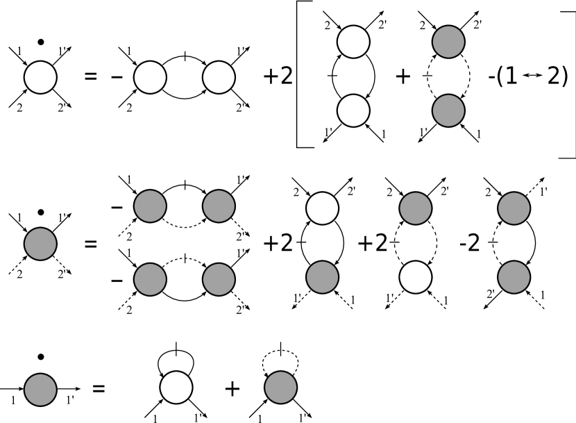
Figure 1: Flow equation diagrams of the four-point vertices and the self-energies. Dashed and full lines are the propagators for the $\tau=A$ and $\tau=B$ orbitals, respectively. White (filled) 4-armed circles are the intra-orbital (inter-orbital) four-point vertices. Propagators with a vertical dash denote single-scale propagators defined via Eq. (2p) and the circular dot on the l.h.s. denotes differentiation with respect to the cutoff $\Lambda$.

4.1 Four-point vertices

The frequency-independent intra-orbital interaction is completely specified by the interaction constants $U_{A}$ and $U_{B}$. Furthermore, in absence of a magnetic field and of a direct hybridization of the two orbitals, the $SU(2)$ spin symmetry allows only two types of inter-orbital interaction: a charge interaction which is specified by $U_{AB}$ and a Hund-type spin interaction of magnitude $J$. We can thus write the properly anti-symmetrized four-point vertex as follows,

$$\gamma_{\Lambda}^{(4)}=\gamma_{\Lambda}^{\rm inter}+\gamma_{\Lambda}^{\rm intra}\,,$$ (2qu)

with ($\delta_{\sigma_{1}\sigma_{2}}$ denote Kronecker deltas)

$$\gamma_{\Lambda}^{\rm inter} =\sum_{\tau=A,B}U^{\Lambda}_{\tau}\delta_{\tau_{1}\tau}\delta_{\tau_{2}\tau}\delta_{\tau_{1}\tau_{1}^{\prime}}\delta_{\tau_{2}\tau_{2}^{\prime}}$$ (2qva)

$$\quad\times\big{(}\delta_{\sigma_{1}\sigma_{1}^{\prime}}\delta_{\sigma_{2}\sigma_{2}^{\prime}}-\delta_{\sigma_{1}\sigma_{2}^{\prime}}\delta_{\sigma_{2}\sigma_{1}^{\prime}}\big{)}\,,$$

$$\gamma_{\Lambda}^{\rm intra} =\big{(}\delta_{\tau_{1}A}\delta_{\tau_{2}B}+\delta_{\tau_{1}B}\delta_{\tau_{2}A}\big{)}\Big{\{}\frac{U^{\Lambda}_{AB}}{2}\big{(}\delta_{\sigma_{1}\sigma_{1}^{\prime}}\delta_{\sigma_{2}\sigma_{2}^{\prime}}\delta_{\tau_{1}\tau_{1}^{\prime}}\delta_{\tau_{2}\tau_{2}^{\prime}}$$ (2qvb)

$$\quad-\delta_{\sigma_{1}\sigma_{2}^{\prime}}\delta_{\sigma_{2}\sigma_{1}^{\prime}}\delta_{\tau_{1}\tau_{2}^{\prime}}\delta_{\tau_{2}\tau_{1}^{\prime}}\big{)}+\frac{J_{\Lambda}}{4}\big{(}{\bm{\sigma}}_{\sigma_{1}\sigma_{1}^{\prime}}\cdot{\bm{\sigma}}_{\sigma_{2}\sigma_{2}^{\prime}}\delta_{\tau_{1}\tau_{1}^{\prime}}\delta_{\tau_{2}\tau_{2}^{\prime}}$$

$$\quad-{\bm{\sigma}}_{\sigma_{1}\sigma_{2}^{\prime}}\cdot{\bm{\sigma}}_{\sigma_{2}\sigma_{1}^{\prime}}\delta_{\tau_{1}\tau_{2}^{\prime}}\delta_{\tau_{2}\tau_{1}^{\prime}}\big{)}\Big{\}}\,.$$

where we dropped the arguments of the vertices, e.g. we implied $\gamma_{\Lambda}^{\rm inter}=\gamma_{\Lambda}^{\rm inter}(1^{\prime},2^{\prime};2,1)$ etc. These are all possible static two-particle correlations in presence of SU(2) symmetry and for two orbitals, in absence of a single particle hybridization of the two dots.

4.2 Flow equations

Fig. 1 shows a diagrammatic representation of the flow equations for the two-point and four-point vertices. The flow equation of $E_{\tau\sigma}^{\Lambda}$ directly follows from the flow equation of the self-energy Eq. (2o), together with the form of the four-point vertex in Eqs. (2qva) and (2qvb). We keep here a $\sigma$-dependence of the self-energy which arises in presence of a magnetic field. We find

$$\partial_{\Lambda}E^{\Lambda}_{\tau\sigma} =\frac{E^{\Lambda}_{\tau{\bar{\sigma}}}U^{\Lambda}_{\tau}/\pi}{(E^{\Lambda}_{\tau{\bar{\sigma}}})^{2}+(\Lambda+\Gamma_{\tau})^{2}}$$ (2qvw)

$$\quad+\frac{E^{\Lambda}_{\bar{\tau}\sigma}(U^{\Lambda}_{AB}+J_{\Lambda}/2)/(2\pi)}{(E^{\Lambda}_{\bar{\tau}\sigma})^{2}+(\Lambda+\Gamma_{\bar{\tau}})^{2}}$$

$$\quad+\frac{E^{\Lambda}_{\bar{\tau}\bar{\sigma}}(U^{\Lambda}_{AB}-J_{\Lambda}/2)/(2\pi)}{(E^{\Lambda}_{\bar{\tau}\bar{\sigma}})^{2}+(\Lambda+\Gamma_{\bar{\tau}})^{2}}\,.$$

The flow equations of the coupling constants which parametrize the four-point vertex follow from Eq. (2qs). For small magnetic fields, we neglect the effect of the magnetic field on the four-point vertex, since these yield corrections in the self-energy of only second or higher order in the magnetic field. We thus replace the $\sigma$-dependent energy levels $E_{\tau\sigma}^{\Lambda}$ by the average value $E_{\tau}^{\Lambda}=(E_{\tau\uparrow}^{\Lambda}+E_{\tau\downarrow}^{\Lambda})/2$ in the flow of the four-point vertex and arrive at

$$\partial_{\Lambda}U^{\Lambda}_{\tau} =\frac{2\big{(}E^{\Lambda}_{\tau}U^{\Lambda}_{\tau}\big{)}^{2}}{\pi\big{[}(E^{\Lambda}_{\tau})^{2}+(\Lambda+\Gamma_{\tau})^{2}\big{]}^{2}}$$ (2qvxa)

$$\quad+\frac{[(E^{\Lambda}_{\bar{\tau}})^{2}-(\Lambda+\Gamma_{\bar{\tau}})^{2}][\frac{3}{4}{J_{\Lambda}}^{2}-(U^{\Lambda}_{AB})^{2}]}{2\pi\big{[}(E^{\Lambda}_{\bar{\tau}})^{2}+(\Lambda+\Gamma_{\bar{\tau}})^{2}\big{]}^{2}}\,,$$

$$\partial_{\Lambda}U^{\Lambda}_{AB} =-\sum_{\tau=A,B}\frac{\big{[}(E^{\Lambda}_{\tau})^{2}-(\Lambda+\Gamma_{\tau})^{2}\big{]}U^{\Lambda}_{\tau}U^{\Lambda}_{AB}}{\pi\big{[}(E^{\Lambda}_{\tau})^{2}+(\Lambda+\Gamma_{\tau})^{2}\big{]}^{2}}$$ (2qvxb)

$$+\frac{[3E^{\Lambda}_{A}E^{\Lambda}_{B}-(\Lambda+\Gamma_{A})(\Lambda+\Gamma_{B})][\frac{3}{4}{J_{\Lambda}}^{2}+(U^{\Lambda}_{AB})^{2}]}{2\pi\big{[}(E^{\Lambda}_{A})^{2}+(\Lambda+\Gamma_{A})^{2}\big{]}\big{[}(E^{\Lambda}_{B})^{2}+(\Lambda+\Gamma_{B})^{2}\big{]}}\,,$$

$$\partial_{\Lambda}J_{\Lambda} =\sum_{\tau=A,B}\frac{\big{[}(E_{\tau}^{\Lambda})^{2}-(\Lambda+\Gamma_{\tau})^{2}\big{]}U^{\Lambda}_{\tau}J_{\Lambda}}{\pi\big{[}(E^{\Lambda}_{\tau})^{2}+(\Lambda+\Gamma_{\tau})^{2}\big{]}^{2}}$$ (2qvxc)

$$+\frac{2E^{\Lambda}_{A}E^{\Lambda}_{B}J_{\Lambda}U^{\Lambda}_{AB}-(\Lambda+\Gamma_{A})(\Lambda+\Gamma_{B}){J_{\Lambda}}^{2}/2}{\pi\big{[}(E^{\Lambda}_{A})^{2}+(\Lambda+\Gamma_{A})^{2}\big{]}\big{[}(E^{\Lambda}_{B})^{2}+(\Lambda+\Gamma_{B})^{2}\big{]}}\,.$$

where $\bar{\tau}=B$ for $\tau=A$ and vice versa.

5 Results

We have solved the flow equations (2qvw-2qvxc) numerically, starting from a very large cutoff $\Lambda_{0}$ and integrating the flow equations to $\Lambda=0$. As discussed in Ref. [15], the appropriate initial values at $\Lambda_{0}\to\infty$ of the flow parameters are

$$E_{\tau\sigma}^{\Lambda_{0}} =E_{\tau\sigma}\,,$$ (2qvxya)

$$U_{\tau}^{\Lambda_{0}} =U_{\tau}\,,$$ (2qvxyb)

$$U_{AB}^{\Lambda_{0}} =U_{AB}\,,\,$$ (2qvxyc)

$$J_{\Lambda_{0}} =J\,.$$ (2qvxyd)

In particular, the bare one-particle contribution arising from the $U_{AB}$ and $U_{A/B}$ terms in Eq. (1) are exactly canceled when integrating the flow equations from $\Lambda=\infty$ to a large but finite $\Lambda_{0}$.[15] We limit the discussion to cases with a ferromagnetic coupling $J<0$, for which the singlet-triplet crossover can be observed. While in most cases the flows are free of divergences, for parameter sets corresponding to strong triplet coupling, the interaction coupling constants diverge for $\Lambda\to 0$. This divergence is probably an artefact of the approximation, in which dynamic and three-particle correlations are ignored. Similar divergences appear in some quantum dot geometries even in absence of Hund’s coupling terms.[23]

Fig. 2 shows the dependence of the conductance for two different values of the level splitting, $\delta=0.5U$ (curve 1) and $\delta=0.4U$ (curve 2), as a function of the gate voltage $V_{g}$ which shifts the energy levels according to Eqs. (2). For large $\delta$ one observes two well separated conductance plateaus which each arise from the usual spin-$1/2$ Kondo effect. In the first plateau region the occupation of the lowest orbital is one while the upper orbital is empty. In the second plateau region the lowest orbital is fully occupied whereas the upper orbital is singly occupied. Around $V_{g}=0$ the occupancy of the lower orbital is close to two (singlet) whereas the upper orbital is almost empty. This leads to a strongly suppressed conductance at and around $V_{g}=0$. A slightly smaller value of the level splitting $\delta$ induces a singlet-triplet transition which leads to the occurrence of a conductance plateau with $G\approx 4e^{2}/h$ around $V_{g}=0$.

While our approach does not allow to calculate the temperature dependence of the conductance, we can investigate its field dependence (at zero temperature) to study the stability of the observed conductance plateaus since a small magnetic field suppresses the Kondo effect in a smilar manner as a finite temperature. The peak of the conductance at $V_{g}=0$ is clearly rather fragile, a small magnetic field cuts the peak in half (curve 4) while the regular $S=1/2$ Kondo plateau hardly changes for comparable values of the magnetic field (curve 3). We can in fact define a Kondo scale as e.g. the value of Zeeman splitting $h$ produced by a magnetic field necessary to suppress conductance by a factor of 1/2.

If the level separation is made very small and close to $V_{g}\approx 0$, eventually all coupling constants diverge when $\Lambda$ approaches zero. The divergence of the parameters, which would presumably disappear in a more refined approximation,[23] is however such that they define a triplet state.

As we already mentioned, one of the main advantages of FRG over NRG is the ability to reliably calculate zero-frequency properties very quickly. One can thus scan large parts of the parameter space to produce 2D maps such as the one in Fig. 3. It shows the conductance as a function of $V_{g}$ and Zeeman splitting $h$. Here, one sees again how the triplet plateau is suppressed at a lower value of $h$ than the $S=1/2$ plateau. Since $U_{A}=U_{B}$, the conductance is symmetric around $V_{g}=0$ and it is thus sufficient to plot for $V_{g}>0$.

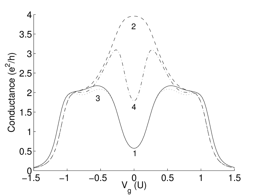
Figure 2: Conductance as a function of the gate voltage $V_{g}$ for $U_{A}=U_{B}=U_{AB}=U$, $J=-0.3U$, $\Gamma_{A}=\Gamma_{B}=0.02\pi U$. A small change in level separation pushes the system into the triplet configuration. (Curves 1 and 2, $\delta=0.5U,0.4U$, respectively.) Adding a small magnetic field, one sees that the triplet conduction peak is much more fragile than the regular Kondo $S=1/2$ plateaus. ($1\rightarrow 3$, $2\rightarrow 4$.)

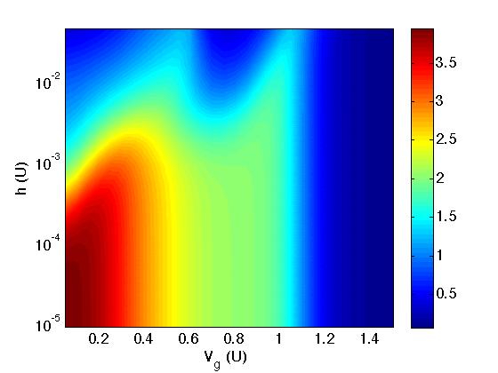
Figure 3: Conductance as a function of gate voltage $V_{g}$ and magnetic field splitting $h$, $\delta=0.4U$. Here it is very clear how the singlet-triplet plateau is suppressed at smaller $h$ than the $S=1/2$ Kondo plateau.

Figure 4 shows the conduction at the symmetry point $V_{g}=0$ as a function of the level separation $\delta$, for different values of magnetic field $H$. As seen by the curve corresponding to $H=0$ (curve 1), this regime of $\delta$ covers the singlet-triplet transition. Even a very small magnetic field suppresses the conduction on the triplet side strongly, but at the transition, a conduction peak remains. The dashed line is an asymptote taken from Eq. (2j), valid for large $\delta$. The derivation of the asymptotic result Eq. (2j) does however only take into account the triplet and local singlet configuration of the quantum dot and becomes inaccurate for too large $\delta$. As before, we also plot the results on a 2D map, shown in Fig. 5.

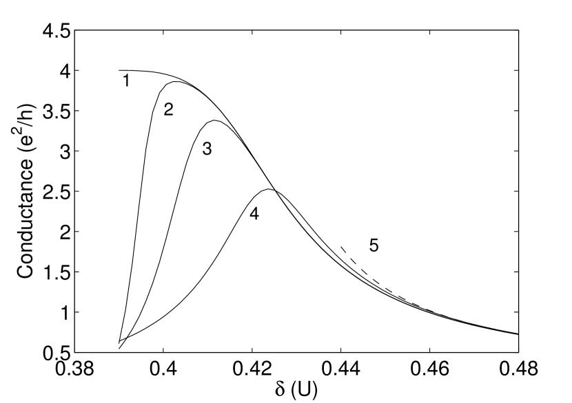
Figure 4: Singlet-triplet transition for $h/U=0,10^{-4},10^{-3},8\times 10^{-3}$ (curves 1-4). Dashed curve (5) is a fit according to Eq. (2j).

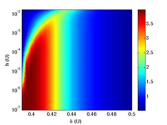
Figure 5: Singlet-triplet transition as a function of $h$. One can see how the conduction on the triplet side gets suppressed and a peak at the singlet-triplet transition remains. The swerve of the peak to higher $\delta$ at the top of the plot is because the magnetic splitting $h$ is becoming comparable to the $x$-axis unit.

To further illustrate the aforementioned triplet divergence of parameters, we plot the conductance for $V_{g}=0$ as a function of $\delta$ and $J$ in Fig. 6. The black dots mark spots where the flow diverged, clearly showing that this occurs when the system is strongly defined to be in the triplet state, with small $\delta$ and large $|J|$. The flow of the parameters is visualized in Fig. 7 for three sets of initial parameters. The top plot shows the flow on the singlet side of the transition, the middle one on the triplet side but still close to the transition, and the bottom one far into the triplet side, where the divergence occurs. But, as stated before, the parameters diverge in a controlled way: $|J|$ and $U_{A},U_{B}$ become very large ($J$ stays negative) while $U_{A}B$ goes to zero, so it is clearly preferable to have the two electrons in the triplet state.

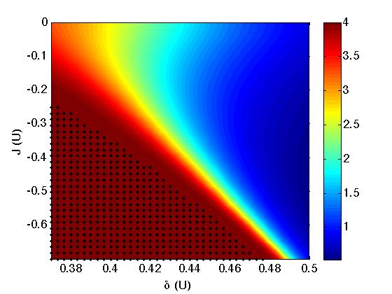
Figure 6: Conductance as a function of $\delta$ and $J$. Direct Coulomb interactions are the standard ones, and we are at the symmetry point $V_{g}=0$. As expected from Eq. (2h), there is a linear relation between $\delta$ and $J$ along the singlet-triplet transition curve. However, renormalization effects shift the line such that the slope is not $1/4$ and it does not go through $(\delta,J)=(0,0)$. The slope is about $0.2$ and an extrapolation shows that the curve passes through $J=0$ at $\delta\simeq 0.37U$. The black dots correspond to parameters where the flow diverges.

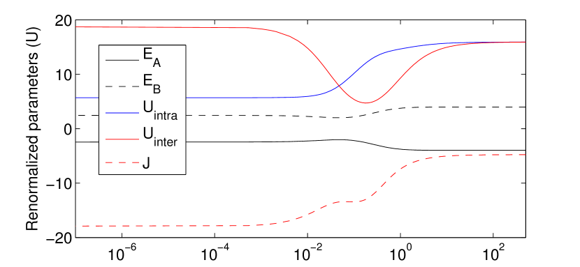
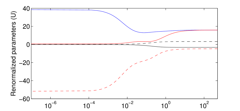
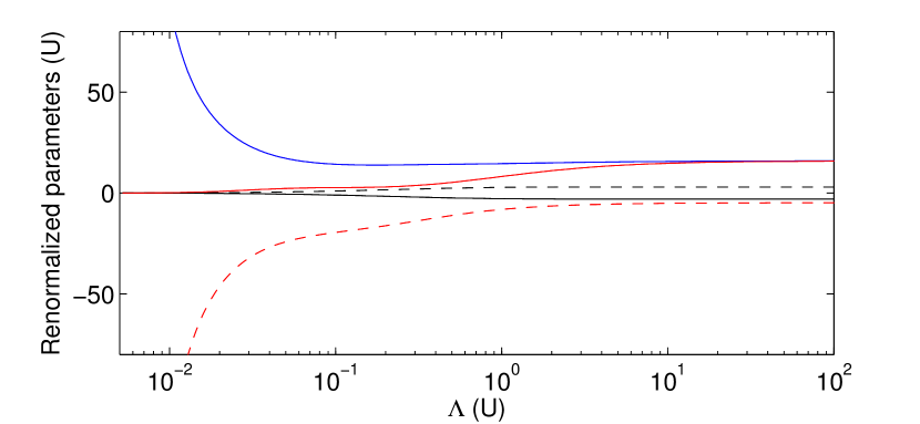
Figure 7: Flow of parameters for $U_{A}=U_{B}=U_{AB}=U$, $J=-0.3U$, $\Gamma_{A}=\Gamma_{B}=0.02\pi U$, $V_{g}=0$. From top to bottom, $\delta=0.5U,0.4U,0.38U$. Top: final value of the inter-orbital Coulomb repulsion is much larger than the intra-orbital one, so it the electrons both stay on the bottom level in the singlet configuration. Middle: The inter-orbital Coulomb repulsion vanishes and the Hund’s exchange grows very large, so the triplet configuration becomes favorable. Bottom: at very small level separation, the flow diverges at some value of $\Lambda$, but at least one can see from the divergence that the system is in the triplet state.

6 Summary and conclusions

In summary, we have extended the static FRG approach presented in Ref. [15] for multi-orbital quantum dots to include also Hund’s coupling and studied the triplet-singlet transition in vertically coupled dots, at $T=0$. Despite its simplicity, the here presented approach reproduces qualitatively the low-temperature results from NRG approaches.[8] The dependence of the conductance on the gate voltage follows the predictions of the perturbative RG analysis [1] near the triplet-singlet transition.

Higher order static correlations would probably give rise to small quantitative improvements, but a discussion of the full temperature and magnetic field dependence of the conductance would require an extension to a dynamic approximation, which, at the moment, are only available for the weak to moderate coupling regime.[12, 13, 14]

N.H. thanks Aldo Isodori and Johannes Bauer for discussions. We acknowledge support from the FP7 IRSES ”SPINMET” grant. E. B. M. acknowledges support from Rannis, the Icelandic Centre for Research. NH further acknowledges support from the DFG-CNPq project 444BRA-113/57/0-1 and the DFG research group FOR 723.

References

• [1] L. I. Glazman and M. E. Raikh, JETP Lett. 47, 452 (1988); T. K. Ng and P. A. Lee, Phys. Rev. Lett. 61, 1768 (1988).
• [2] Y. Meir, K. Hirose and N.S. Wingreen, Phys. Rev. Lett. 89, 196802 (2002).
• [3] S. Sasaki, S. De Franceschi, J. M. Elzerman, W. G. van der Wiel, M. Eto, S. Tarucha, and L. P. Kouwenhoven Nature 405, 764 (2000).
• [4] L. P. Kouwenhoven, D. G. Austing, and S. Tarucha, Rep- Prog. Phys. 64, 701 (2001).
• [5] S. Florens et al., J. Phys.: Condens. Matter 23, 243202 (2011)
• [6] R. Bulla, T. A. Costi, and T. Pruschke, Rev. Mod. Phys. 80, 395 (2008).
• [7] F. Anders et al., Phys. Rev. Lett. 100, 086809 (2008)
• [8] W. Izumida, O. Sakai, and S. Tarucha, Phys. Rev. Lett. 87, 216803 (2001); W. Izumida and O. Sakai, J. Phys. Soc. Jpn. 74, 103 (2005).
• [9] W. Hofstetter and H. Schoeller, Phys. Rev. Lett. 88, 016803 (2001).
• [10] M. Pustilnik, L. I. Glazman, and W. Hofstetter, Phys. Rev. B 68, R161303 (2003).
• [11] W. Hofstetter and G. Zarand, Phys. Rev. B 69, 235301 (2004).
• [12] C. Karrasch, R. Hedden, R. Peters, T. Pruschke, K. Schönhammer, and V. Meden, J. Phys.: Condens. Matter 20, 345205 (2008).
• [13] L. Bartosch, H. Freire, J. J. R. Cardenas, and P. Kopietz, J. Phys. Condens. Matter 21, 305602 (2009).
• [14] A. Isidori, D. Roosen, L. Bartosch, W. Hofstetter, and P. Kopietz, Phys. Rev. B 81, 235120 (2010).
• [15] C. Karrasch, T. Enss and V. Meden, Phys. Rev. B 73, 235337 (2006).
• [16] B. Horváth, B. Lazarovitz, and G. Zaránd, Phys. Rev. B 84, 205117 (2011).
• [17] H. Freire and E. Corrêa, J. Low. Temp. Phys. 166, 192 (2012).
• [18] M. Pustilnik and L.I. Glazman, Phys. Rev. Lett. 85, 2993 (2000); Phys. Rev. B 64, 045328 (2001).
• [19] Y. Meir and N. S. Wingreen, Phys. Rev. Lett. 68, 2512 (1992).
• [20] C. Wetterich, Phys. Lett. B 301, 90 (1993).
• [21] T. R. Morris, Int. J. Mod. Phys. A 9, 2411 (1994).
• [22] W. Metzner, M. Salmhofer, C. Honerkamp, V. Meden, and K. Schönhammer, Rev. Mod. Phys. 84, 299 (2012); P. Kopietz, L. Bartosch, and F. Schütz, “Introduction to the Functional Renormalization Group”, Springer (2010).
• [23] M. Weyrauch and D. Sibold , Phys. Rev. B 77, 125309 (2008).