Recursive co-kriging model for Design of Computer experiments with multiple levels of fidelity with an application to hydrodynamic

abstract

We consider in this paper the problem of building a fast-running approximation - also called surrogate model - of a complex computer code. The co-kriging based surrogate model is a promising tool to build such an approximation when the complex computer code can be run at different levels of accuracy. We present here an original approach to perform a multi-fidelity co-kriging model which is based on a recursive formulation. We prove that the predictive mean and the variance of the presented approach are identical to the ones of the original co-kriging model proposed by [Kennedy, M.C. and O’Hagan, A., Biometrika, 87, pp 1-13, 2000]. However, our new approach allows to obtain original results. First, closed form formulas for the universal co-kriging predictive mean and variance are given. Second, a fast cross-validation procedure for the multi-fidelity co-kriging model is introduced. Finally, the proposed approach has a reduced computational complexity compared to the previous one. The multi-fidelity model is successfully applied to emulate a hydrodynamic simulator.

keywords

: uncertainty quantification, surrogate models, universal co-kriging, recursive model, fast cross-validation, multi-fidelity computer code.

1 Introduction

Computer codes are widely used in science and engineering to describe physical phenomena. Advances in physics and computer science lead to increased complexity for the simulators. As a consequence, to perform a sensitivity analysis or an optimization based on a complex computer code, a fast approximation of it - also called surrogate model - is built in order to avoid prohibitive computational cost. A very popular method to build surrogate model is the Gaussian process regression, also named kriging. It corresponds to a particular class of surrogate models which makes the assumption that the response of the complex code is a realization of a Gaussian process. This method was originally introduced in geostatistics in [Krige, 1951] and it was then proposed in the field of computer experiments in [Sacks et al., 1989]. During the last decades, this method has become widely used and investigated. The reader is referred to the books [Stein, 1999], [Santner et al., 2003] and [Rasmussen and Williams, 2006] for more detail about it.

Sometimes low-fidelity versions of the computer code are available. They may be less accurate but they are computationally cheap. A question of interest is how to build a surrogate model using data from simulations of multiple levels of fidelity. Our objective is hence to build a multi-fidelity surrogate model which is able to use the information obtained from the fast versions of the code. Such models have been presented in the literature [Craig et al., 1998], [Kennedy and O’Hagan, 2000], [Higdon et al., 2004], [Forrester et al., 2007], [Qian and Wu, 2008] and [Cumming and Goldstein, 2009].

The first multi-fidelity model proposed in [Craig et al., 1998] is based on a linear regression formulation. Then this model is improved in [Cumming and Goldstein, 2009] by using a Bayes linear formulation. The reader is referred to [Goldstein and Wooff, 2007] for further detail about the Bayes linear approach. The methods suggested in [Craig et al., 1998] and [Cumming and Goldstein, 2009] have the strength to be relatively computationally clean but as they are based on a linear regression formulation, they could suffer from a lack of accuracy. Another approach is to use an extension of kriging for multiple response models which is called co-kriging. The idea is implemented in [Kennedy and O’Hagan, 2000] which presents a co-kriging model based on an autoregressive relation between the different code levels. This method turns out to be very efficient and it has been applied and extended significantly. In particular, the use of co-kriging for multi-fidelity optimization is presented in [Forrester et al., 2007] and a Bayesian formulation is proposed in [Qian and Wu, 2008].

The strength of the co-kriging model is that it gives very good predictive models but it is often computationally expensive, especially when the number of simulations is large. Furthermore, large data set can generate problems such as ill-conditioned covariance matrices. These problems are known for kriging but they become even more difficult for co-kriging since the total number of observations is the sum of the observations at all code levels.

In this paper, we adopt a new approach for multi-fidelity surrogate modeling which uses a co-kriging model but with an original recursive formulation. In fact, our model is able to build a $s$-level co-kriging model by building $s$ independent krigings. An important property of this model is that it provides predictive mean and variance identical to the ones presented in [Kennedy and O’Hagan, 2000]. However, our approach significantly reduces the complexity of the model since it divides the whole set of simulations into groups of simulations corresponding to the ones of each level. Therefore, we will have $s$ sub-matrices to invert which is less expensive and ill-conditioned than a large one and the estimation of the parameters can be performed separately (Section 2.3).

Furthermore, a strength of our approach is that it allows to extend classical results of kriging to the considered co-kriging model. The two original results presented in our paper are the following ones: First, closed form expressions for the universal co-kriging predictive mean and variance are given (Section 3). Second, the fast cross-validation method proposed in [Dubrule, 1983] is extended to the multi-fidelity co-kriging model (Section 4). Finally, we illustrate these results in a complex hydrodynamic simulator (Section 5).

2 Multi-fidelity Gaussian process regression

In Subsection 2.1, we briefly present the approach to build multi-fidelity model suggested in [Kennedy and O’Hagan, 2000] that uses a co-kriging model. In Subsection 2.2, we detail our recursive approach to build such a model. The recursive formulation of the multi-fidelity model is the first novelty of this paper. We will see in the next sections that the new formulation allows us to find original results about the co-kriging model and to reduce its computational complexity.

2.1 The classical autoregressive model

Let us suppose that we have $s$ levels of code $(z_{t}(x))_{t=1,\dots,s}$ sorted by increasing order of fidelity and modeled by Gaussian processes $(Z_{t}(x))_{t=1,\dots,s}$, $x\in Q$. We hence consider that $z_{s}(x)$ is the most accurate and costly code that we want to surrogate and $(z_{t}(x))_{t=1,\dots,s-1}$ are cheaper versions of it with $z_{1}(x)$ the less accurate one. We consider the following autoregressive model with $t=2,\dots,s$:

$$\left\{\begin{array}[]{l}Z_{t}(x)=\rho_{t-1}(x)Z_{t-1}(x)+\delta_{t}(x)\\ Z_{t-1}(x)\perp\delta_{t}(x)\\ \rho_{t-1}(x)=g_{t-1}^{T}(x)\beta_{\rho_{t-1}}\\ \end{array}\right.$$ (1)

where:

$$\delta_{t}(x)\sim\mathcal{GP}(f_{t}^{T}(x)\beta_{t},\sigma_{t}^{2}r_{t}(x,x^{\prime}))$$ (2)

and:

$$Z_{1}(x)\sim\mathcal{GP}(f_{1}^{T}(x)\beta_{1},\sigma_{1}^{2}r_{1}(x,x^{\prime}))$$ (3)

Here, ^T stands for the transpose, $\perp$ denotes the independence relationship, $\mathcal{GP}$ stands for Gaussian Process, $g_{t-1}(x)$ is a vector of $q_{t-1}$ regression functions, $f_{t}(x)$ is a vector of $p_{t}$ regression functions, $r_{t}(x,x^{\prime})$ is a correlation function, $\beta_{t}$ is a $p_{t}$-dimensional vector, $\beta_{\rho_{t-1}}$ is a $q_{t-1}$-dimensional vector, and $\sigma_{t}^{2}$ is a real. Since we suppose that the responses are realizations of Gaussian processes, the multi-fidelity model can be built by conditioning by the known responses of the codes at the different levels.

The previous model comes from the article [Kennedy and O’Hagan, 2000]. It is induced by the following assumption: $\forall x\in Q$, if we know $Z_{t-1}(x)$, nothing more can be learned about $Z_{t}(x)$ from $Z_{t-1}(x^{\prime})$ for $x\neq x^{\prime}$.

Let us consider $\mathcal{Z}^{(s)}=(\mathcal{Z}_{1}^{T},\dots,\mathcal{Z}_{s}^{T})^{T}$ the Gaussian vector containing the values of the random processes $(Z_{t}(x))_{t=1,\dots,s}$ at the points in the experimental design sets $(D_{t})_{t=1,\dots,s}$ with $D_{s}\subseteq D_{s-1}\subseteq\dots\subseteq D_{1}$. We denote by $z^{(s)}=(z_{1}^{T},\dots,z_{s}^{T})^{T}$ the vector containing the values of $(z_{t}(x))_{t=1,\dots,s}$ at the points in $(D_{t})_{t=1,\dots,s}$. The nested property of the experimental design sets is not necessary to build the model but it allows for a simple estimation of the model parameters. Since the codes are sorted in increasing order of fidelity it is not an unreasonable constraint for practical applications. By denoting $\beta=(\beta_{1}^{T},\dots,\beta_{s}^{T})^{T}$ the trend parameters, $\beta_{\rho}=(\beta_{\rho_{1}}^{T},\dots,\beta_{\rho_{s-1}}^{T})^{T}$ the trend of the adjustment parameters and $\sigma^{2}=(\sigma_{1}^{2},\dots,\sigma_{s}^{2})$ the variance parameters, we have for any $x\in Q$:

$$[Z_{s}(x)|\mathcal{Z}^{(s)}=z^{(s)},\beta,\beta_{\rho},\sigma^{2}]\sim\mathcal{N}\left(m_{Z_{s}}(x),s_{Z_{s}}^{2}(x)\right)$$

where:

$$m_{Z_{s}}(x)=h_{s}(x)^{T}\beta+t_{s}(x)^{T}V_{s}^{-1}(z^{(s)}-H_{s}\beta)$$ (4)

and:

$$s_{Z_{s}}^{2}(x)=v_{Z_{s}}^{2}(x)-t_{s}(x)^{T}V_{s}^{-1}t_{s}(x)$$ (5)

The Gaussian process regression mean $m_{Z_{s}}(x)$ is the predictive model of the highest fidelity response $z_{s}(x)$ which is built with the known responses of all code levels $z^{(s)}$. The variance $s_{Z_{s}}^{2}(x)$ represents the predictive mean squared error of the model.

The matrix $V_{s}$ is the covariance matrix of the Gaussian vector $\mathcal{Z}^{(s)}$, the vector $t_{s}(x)$ is the vector of covariances between $Z_{s}(x)$ and $\mathcal{Z}^{(s)}$, $H_{s}\beta$ is the mean of $\mathcal{Z}^{(s)}$, $h_{s}(x)^{T}\beta$ is the mean of $Z_{s}(x)$ and $v_{Z_{s}}^{2}(x)$ is the variance of $Z_{s}(x)$. All these terms are built in terms of the experience vector at level $t$ (6) and of the covariance between $Z_{t}(x)$ and $Z_{t^{\prime}}(x)$:

$$h_{t}(x)^{T}=\left(\left(\prod_{i=1}^{t-1}{\rho_{i}(x)}\right)f_{1}^{T}(x),\left(\prod_{i=2}^{t-1}{\rho_{i}(x)}\right)f_{2}^{T}(x),\dots,\rho_{t-1}(x)f_{t-1}^{T}(x),f_{t}^{T}(x)\right)$$ (6)

$$\mathrm{cov}(Z_{t}(x),Z_{t^{\prime}}(x^{\prime})|\sigma^{2},\beta,\beta_{\rho})=\left(\prod_{i=t^{\prime}}^{t-1}\rho_{i}(x)\right)\mathrm{cov}(Z_{t^{\prime}}(x),Z_{t^{\prime}}(x^{\prime})|\sigma^{2},\beta,\beta_{\rho})$$ (7)

and:

$$\mathrm{cov}(Z_{t}(x),Z_{t}(x^{\prime})|\sigma^{2},\beta,\beta_{\rho})=\sum_{j=1}^{t}{\sigma_{j}^{2}\left(\prod_{i=j}^{t-1}{\rho_{i}(x)\rho_{i}(x^{\prime})}\right)r_{j}(x,x^{\prime})}$$ (8)

Remark.

The model (1) is an extension of the model presented in [Kennedy and O’Hagan, 2000] in which the adjustment parameters $\rho_{t}(x)_{t=2,\dots,s}$ do not depend on $x$. We show in a practical application (Section 5) that this extension is worthwhile.

2.2 Recursive multi-fidelity model

In this section, we present the new multi-fidelity model which is based on a recursive formulation. Let us consider the following model for $t=2,\dots,s$ :

$$\left\{\begin{array}[]{l}Z_{t}(x)=\rho_{t-1}(x)\tilde{Z}_{t-1}(x)+\delta_{t}(x)\\ \tilde{Z}_{t-1}(x)\perp\delta_{t}(x)\\ \rho_{t-1}(x)=g_{t-1}^{T}(x)\beta_{\rho_{t-1}}\\ \end{array}\right.$$ (9)

where $\tilde{Z}_{t-1}(x)$ is a Gaussian process with distribution $[Z_{t-1}(x)|\mathcal{Z}^{(t-1)}=z^{(t-1)},\beta_{t-1},\beta_{\rho_{t-2}},\sigma_{t-1}^{2}]$, $\delta_{t}(x)$ is a Gaussian process with distribution (2) and $D_{s}\subseteq D_{s-1}\subseteq\dots\subseteq D_{1}$. The unique difference with the previous model is that we express $Z_{t}(x)$ (the Gaussian process modeling the response at level $t$) as a function of the Gaussian process $Z_{t-1}(x)$ conditioned by the values $z^{(t-1)}=(z_{1},\dots,z_{t-1})$ at points in the experimental design sets $(D_{i})_{i=1,\dots,t-1}$. As in the previous model, the nested property for the experimental design sets is assumed because it allows for efficient estimations of the model parameters. The Gaussian processes $(\delta_{t}(x))_{t=2,\dots,s}$ have the same definition as previously and we have for $t=2,\dots,s$ and for $x\in Q$:

$$\left[Z_{t}(x)|\mathcal{Z}^{(t)}=z^{(t)},\beta_{t},\beta_{\rho_{t-1}},\sigma_{t}^{2}\right]\sim\mathcal{N}\left(\mu_{Z_{t}}(x),s_{Z_{t}}^{2}(x)\right)$$ (10)

where:

$$\mu_{Z_{t}}(x)=\rho_{t-1}(x)\mu_{Z_{t-1}}(x)+f_{t}^{T}(x)\beta_{t}+r_{t}^{T}(x)R_{t}^{-1}\left(z_{t}-\rho_{t-1}(D_{t})\odot z_{t-1}(D_{t})-F_{t}\beta_{t}\right)$$ (11)

and:

$$\sigma_{Z_{t}}^{2}(x)=\rho_{t-1}^{2}(x)\sigma_{Z_{t-1}}^{2}(x)+\sigma_{t}^{2}\left(1-r_{t}^{T}(x)R_{t}^{-1}r_{t}(x)\right)$$ (12)

The notation $\odot$ represents the element by element matrix product. $R_{t}$ is the correlation matrix $R_{t}=(r_{t}(x,x^{\prime}))_{x,x^{\prime}\in D_{t}}$ and $r_{t}^{T}(x)$ is the correlation vector $r_{t}^{T}(x)=(r_{t}(x,x^{\prime}))_{x^{\prime}\in D_{t}}$. We denote by $\rho_{t}(D_{t-1})$ the vector containing the values of $\rho_{t}(x)$ for $x\in D_{t-1}$, $z_{t}(D_{t-1})$ the vector containing the known values of $Z_{t}(x)$ at points in $D_{t-1}$ and $F_{t}$ is the experience matrix containing the values of $f_{t}(x)^{T}$ on $D_{t}$.

The mean $\mu_{Z_{t}}(x)$ is the surrogate model of the response at level $t$, $1\leq t\leq s$, taking into account the known values of the $t$ first levels of responses $(z_{i})_{i=1,\dots,t}$ and the variance $\sigma_{Z_{t}}^{2}(x)$ represents the mean squared error of this model. The mean and the variance of the Gaussian process regression at level $t$ being expressed in function of the ones of level $t-1$, we have a recursive multi-fidelity metamodel. Furthermore, in this new formulation, it is clearly emphasized that the mean of the predictive distribution does not depend on the variance parameters $(\sigma_{t}^{2})_{t=1,\dots,s}$. This is a classical result of kriging which states that for covariance kernels of the form $k(x,x^{\prime})=\sigma^{2}r(x,x^{\prime})$, the mean of the kriging model is independent of $\sigma^{2}$. Another important strength of the recursive formulation is that contrary to the formulation suggested in [Kennedy and O’Hagan, 2000], once the multi-fidelity model is built, it provides the surrogate models of all the responses $(z_{t}(x))_{t=1\dots,s}$.

We have the following proposition.

Proposition 1

Let us consider $s$ Gaussian processes $(Z_{t}(x))_{t=1,\dots,s}$ and $\mathcal{Z}^{(s)}=(\mathcal{Z}_{t})_{t=1,\dots,s}$ the Gaussian vector containing the values of $(Z_{t}(x))_{t=1,\dots,s}$ at points in $(D_{t})_{t=1,\dots,s}$ with $D_{s}\subseteq D_{s-1}\subseteq\dots\subseteq D_{1}$. If we consider the mean and the variance (4) and (5) induced by the model (1) when we condition the Gaussian process $Z_{s}(x)$ by the known values $z^{(s)}$ of $\mathcal{Z}^{(s)}$ and by the parameters $\beta$, $\beta_{\rho}$ and $\sigma^{2}$ and the mean and the variance (11) and (12) induced by the model (9) when we condition $Z_{s}(x)$ by $z^{(s)}$ and by the parameters $\beta$, $\beta_{\rho}$ and $\sigma^{2}$, then, we have:

$$\mu_{Z_{s}}(x) = m_{Z_{s}}(x)$$

$$\sigma_{Z_{s}}^{2}(x) = s_{Z_{s}}^{2}(x)$$

The proof of the proposition is given in Appendix A.1. It shows that the model presented in [Kennedy and O’Hagan, 2000] and the recursive model (9) have the same predictive Gaussian distribution. Our objective in the next sections is to show that the new formulation (9) has several advantages compared to the one of [Kennedy and O’Hagan, 2000]. First, its computational complexity is lower (Section 2.3); second, it provides closed form expressions for the universal co-kriging mean and variance contrarily to [Kennedy and O’Hagan, 2000] (Section 3); third, it makes it possible to implement a fast cross-validation procedure (Section 4).

2.3 Complexity analysis

The computational cost is dominated by the inversion of the covariance matrices. In the original approach proposed in [Kennedy and O’Hagan, 2000] one has to invert the matrix $V_{s}$ of size $\sum_{i=1}^{s}n_{i}\times\sum_{i=1}^{s}n_{i}$.

Our recursive formulation shows that building a $s$-level co-kriging is equivalent to build $s$ independent krigings. This implies a reduction of the model complexity. Indeed, the inversion of $s$ matrices $(R_{t})_{t={1,\dots,s}}$ of size $(n_{t}\times n_{t})_{t={1,\dots,s}}$ where $n_{t}$ corresponds to the size of the vector $z_{t}$ at level $t=1,\dots,s$ is less expensive than the inversion of the matrix $V_{s}$ of size $\sum_{i=1}^{s}n_{i}\times\sum_{i=1}^{s}n_{i}$. We also reduce the memory cost since storing the $s$ matrices $(R_{t})_{t={1,\dots,s}}$ requires less memory than storing the matrix $V_{s}$. Finally, we note that the model with this formulation is more interpretable since we can deduce the impact of each level of response into the model error through $(\sigma_{Z_{t}}^{2}(x))_{t={1,\dots,s}}$.

2.4 Parameter estimation

We present in this section a Bayesian estimation of the parameter $\psi=(\beta,\beta_{\rho},\sigma^{2})$ focusing on conjugate and non-informative distributions for the priors. This allows us to obtain closed form expressions for the estimations of the parameters. Furthermore, from the non-informative case, we can obtain the estimates given by a maximum likelihood method. The presented formulas can hence be used in a frequentist approach. We note that the recursive formulation and the nested property of the experimental designs allow for separate the estimations of the parameters $(\beta_{t},\beta_{\rho_{t-1}},\sigma^{2}_{t})_{t=1,\dots,s}$ and $(\beta_{1},\sigma_{1}^{2})$.

We address two cases in this section

• Case (i): all the priors are informative

• Case (ii): all the priors are non-informative

It is of course be possible to address the case of a mixture of informative and non-informative priors. For the non-informative case (ii), we use the “Jeffreys priors” [Jeffreys, 1961]:

$$p(\beta_{1}|\sigma_{1}^{2})\propto 1,\quad p(\sigma_{1}^{2})\propto\frac{1}{\sigma_{1}^{2}},\quad p(\beta_{\rho_{t-1}},\beta_{t}|z^{(t-1)},\sigma_{t}^{2})\propto 1,\quad p(\sigma_{t}^{2}|z^{(t-1)})\propto\frac{1}{\sigma_{t}^{2}}$$ (13)

where $t=2,\dots,s$. For the informative case (i), we consider the following conjugate prior distributions:

$$[\beta_{1}|\sigma_{1}^{2}]\sim\mathcal{N}_{p_{1}}(b_{1},\sigma_{1}^{2}V_{1})$$

$$[\beta_{\rho_{t-1}},\beta_{t}|z^{(t-1)},\sigma_{t}^{2}]\sim\mathcal{N}_{q_{t-1}+p_{t}}\left(b_{t}=\left(\begin{array}[]{c}b^{\rho}_{t-1}\\ b^{\beta}_{t}\end{array}\right),\sigma_{t}^{2}V_{t}=\sigma_{t}^{2}\left(\begin{array}[]{cc}V^{\rho}_{t-1}&0\\ 0&V^{\beta}_{t}\\ \end{array}\right)\right)$$

$$[\sigma_{1}^{2}]\sim\mathcal{IG}(\alpha_{1},\gamma_{1}),\qquad[\sigma_{t}^{2}|z^{(t-1)}]\sim\mathcal{IG}(\alpha_{t},\gamma_{t})$$

with $b_{1}$ a vector a size $p_{1}$, $b^{\rho}_{t-1}$ a vector of size $q_{t-1}$, $b^{\beta}_{t}$ a vector of size $p_{t}$, $V_{1}$ a $p_{1}\times p_{1}$ matrix, $V^{\rho}_{t-1}$ a $q_{t-1}\times q_{t-1}$ matrix, $V^{\beta}_{t}$ a $p_{t}\times p_{t}$ matrix, $\alpha_{1},\gamma_{1},\alpha_{t},\gamma_{t}>0$ and $\mathcal{IG}$ stands for the inverse Gamma distribution. These informative priors allow the user to prescribe the prior means and variances of all parameters. The choice of conjugate priors allows us to have closed form expressions for the posterior distributions of the parameters. Indeed, we have:

$$[\beta_{1}|z_{1},\sigma_{1}^{2}]\sim\mathcal{N}_{p_{1}}(\Sigma_{1}\nu_{1},\Sigma_{1})\qquad[\beta_{\rho_{t-1}},\beta_{t}|z^{(t)},\sigma_{t}^{2}]\sim\mathcal{N}_{q_{t-1}+q_{t}}(\Sigma_{t}\nu_{t},\Sigma_{t})$$ (14)

where, for $t\geq 1$:

$$\Sigma_{t}=\left\{\begin{array}[]{lr}[H_{t}^{T}\frac{R_{t}^{-1}}{\sigma_{2}^{2}}H_{t}+\frac{V_{t}^{-1}}{\sigma_{2}^{2}}]^{-1}&\mathbf{(i)}\\ [H_{t}^{T}\frac{R_{t}^{-1}}{\sigma_{2}^{2}}H_{t}]^{-1}&\mathbf{(ii)}\\ \end{array}\right.\nu_{t}=\left\{\begin{array}[]{lr}[H_{t}^{T}\frac{R_{t}^{-1}}{\sigma_{2}^{2}}z_{t}+\frac{V_{t}^{-1}}{\sigma_{2}^{2}}b_{t}]&\mathbf{(i)}\\ [H_{t}^{T}\frac{R_{t}^{-1}}{\sigma_{2}^{2}}z_{t}]&\mathbf{(ii)}\\ \end{array}\right.$$ (15)

with $H_{1}=F_{1}$ and for $t>1$, $H_{t}=[G_{t-1}\odot(z_{t-1}(D_{t})\mathbf{1}^{T}_{q_{t-1}})\quad F_{t}]$ where $G_{t-1}$ is the experience matrix containing the values of $g_{t-1}(x)^{T}$ in $D_{t}$ and $\mathbf{1}^{T}_{q_{t-1}}$ is a $q_{t-1}$-vector of ones. Furthermore, we have for $t\geq 1$:

$$[\sigma_{t}^{2}|z^{(t)}]\sim\mathcal{IG}(a_{t},\frac{Q_{t}}{2})$$ (16)

where:

$$Q_{t}=\left\{\begin{array}[]{lr}\gamma_{t}+(b_{t}-\hat{\lambda}_{t})^{T}(V_{t}+[H_{t}^{T}R_{t}^{-1}H_{t}]^{-1})^{-1}(b_{t}-\hat{\lambda}_{t})+\hat{Q}_{t}&\mathbf{(i)}\\ \hat{Q}_{t}&\mathbf{(ii)}\\ \end{array}\right.$$

with $\hat{Q}_{t}=(z_{t}-H_{t}\hat{\lambda}_{t})^{T}R_{t}^{-1}(z_{t}-H_{t}\hat{\lambda}_{t})$ , $\hat{\lambda}_{t}=(H_{t}^{T}R_{t}^{-1}H_{t}F)^{-1}H_{t}^{T}R_{t}^{-1}z_{t}$ and :

$$a_{t}=\left\{\begin{array}[]{lr}\frac{n_{t}}{2}+\alpha_{t}&\mathbf{(i)}\\ \frac{n_{t}-p_{t}-q_{t-1}}{2}&\mathbf{(ii)}\\ \end{array}\right.$$

with the convention $q_{0}=0$.

We highlight that the maximum likelihood estimators for the parameters $\beta_{1}$ and $(\beta_{\rho_{t-1}},\beta_{t})$ are given by the means of the posterior distributions of the Bayesian estimations in the non-informative case. Furthermore, the restricted maximum likelihood estimate of the variance parameter $\sigma_{t}^{2}$ can also be deduced from the posterior distribution of the Bayesian estimation in the non-informative case and is given by $\hat{\sigma}_{t,\mathrm{EML}}^{2}=\frac{Q_{t}}{2a_{t}}$. The restricted maximum likelihood estimation is a method which allows to reduce the bias of the maximum likelihood estimation [Patterson and Thompson, 1971].

3 Universal co-kriging model

We can see in equation (10) that the predictive distribution of $Z_{s}(x)$ is conditioned by the observations $z^{(s)}$ and the parameters $\beta$, $\beta_{\rho}$ and $\sigma^{2}$. The objective of a Bayesian prediction is to integrate the uncertainty due to the parameter estimations into the predictive distribution. Indeed, in the previous subsection, we have expressed the posterior distributions of the variance parameters $(\sigma_{t}^{2})_{t=1,\dots,s}$ conditionally to the observations and the posterior distributions of the trend parameters $\beta_{1}$ and $(\beta_{\rho_{t-1}},\beta_{t})_{t=2,\dots,s}$ conditionally to the observations and the variance parameters. Thus, using the Bayes formula, we can easily obtain a predictive distribution only conditioned by the observations by integrating into it the posterior distributions of the parameters.

As a result of this integration, the predictive distribution is not Gaussian. In particular, we cannot have a closed form expression for the predictive distribution. However, it is possible to obtain closed form expressions for the posterior mean $\mathbb{E}[Z_{s}(x)|\mathcal{Z}^{(s)}=z^{(s)}]$ and variance $\mathrm{Var}(Z_{s}(x)|\mathcal{Z}^{(s)}=z^{(s)})$.

The following proposition giving the closed form expressions of the posterior mean and variance of the predictive distribution only conditioned by the observations is a novelty. The proof of this proposition is based on the recursive formulation which emphasizes the strength of this new approach. Indeed, it does not seem possible to obtain this result by considering directly the model suggested in [Kennedy and O’Hagan, 2000].

Proposition 2

Let us consider $s$ Gaussian processes $(Z_{t}(x))_{t=1,\dots,s}$ and $\mathcal{Z}^{(s)}=(\mathcal{Z}_{t})_{t=1,\dots,s}$ the Gaussian vector containing the values of $(Z_{t}(x))_{t=1,\dots,s}$ at points in $(D_{t})_{t=1,\dots,s}$ with $D_{s}\subseteq D_{s-1}\subseteq\dots\subseteq D_{1}$. If we consider the conditional predictive distribution in equation (10) and the posterior distributions of the parameters given in equations (14) and (16), then we have for $t=1,\dots,s$:

$$\mathbb{E}[Z_{t}(x)|\mathcal{Z}^{(t)}=z^{(t)}]=h_{t}^{T}(x)\Sigma_{t}\nu_{t}+r_{t}^{T}(x)R_{t}^{-1}\left(z_{t}-H_{t}\Sigma_{t}\nu_{t}\right)$$ (17)

with $h_{1}^{T}=f_{1}^{T}$, $H_{1}=F_{1}$ and for $t>1$, $h_{t}^{T}(x)=\left(\begin{array}[]{lr}g_{t-1}(x)^{T}\mathbb{E}[Z_{t-1}(x)|\mathcal{Z}_{t-1}=z_{t-1}]&f_{t}^{T}(x)\\ \end{array}\right)$ and $H_{t}=[G_{t-1}\odot(z_{t-1}(D_{t})\mathbf{1}^{T}_{q_{t-1}})\quad F_{t}]$. Furthermore, we have:

$$\begin{array}[]{lll}\mathrm{Var}(Z_{t}(x)|\mathcal{Z}^{(t)}=z^{(t)})&=&\hat{\rho}_{t-1}^{2}(x)\mathrm{Var}(Z_{t-1}(x)|\mathcal{Z}^{(t-1)}=z^{(t-1)})+\frac{Q_{t}}{2\left(a_{t}-1\right)}\left(1-r_{t}^{T}(x)R_{t}^{-1}r_{t}^{T}(x)\right)\\ &&+\left(h_{t}^{T}-r_{t}^{T}(x)R_{t}^{-1}H_{t}\right)\Sigma_{t}\left(h_{t}^{T}-r_{t}^{T}(x)R_{t}^{-1}H_{t}\right)^{T}\\ \end{array}$$ (18)

with $\hat{\rho}_{t-1}(x)=[\Sigma_{t}\nu_{t}]_{1,\dots,q_{t-1}}$.

The proof of Proposition 2 is given in Appendix A.2. We note that, in the mean of the predictive distribution, the parameters have been replaced by their posterior means. Furthermore, in the variance of the predictive distribution, the variance parameter has been replaced by its posterior mean and the term $\left(h_{t}^{T}-r_{t}^{T}(x)R_{t}^{-1}H_{t}\right)\Sigma_{t}\left(h_{t}^{T}-r_{t}^{T}(x)R_{t}^{-1}H_{t}\right)^{T}$ has been added. It represents the uncertainty due to the estimation of the regression parameters (including the adjustment coefficient). We call these formulas the universal co-kriging equations due to their similarities with the well-known universal kriging equations (they are identical for $s=1$).

4 Fast cross-validation for co-kriging surrogate models

The idea of a cross-validation procedure is to split the experimental design set into two disjoint sets, one is used for training and the other one is used to monitor the performance of the surrogate model. The idea is that the performance on the test set can be used as a proxy for the generalization error. A particular case of this method is the Leave-One-Out Cross-Validation (noted LOO-CV) where $n$ test sets are obtained by removing one observation at a time. This procedure can be time-consuming for a kriging model but it is shown in [Dubrule, 1983], [Rasmussen and Williams, 2006] and [Zhang and Wang, 2009] that there are computational shortcuts. Our recursive formulation allows to extend these ideas to co-kriging models (which is not possible with the original formulation in [Kennedy and O’Hagan, 2000]). Furthermore, the cross-validation equations proposed in this section extend the previous ones even for $s=1$ (i.e. the classical kriging model) since they do not suppose that the regression and the variance coefficients are known. Therefore, those parameters are re-estimated for each training set. We note that the re-estimation of the variance coefficient is a novelty which is important since fixing this parameter can lead to huge errors for the estimation of the cross-validation predictive variance when the number of observations is small or when the number of points in the test set is important.

If we denote by $\xi_{s}$ the set of indices of $n_{test}$ points in $D_{s}$ constituting the test set $D_{test}$ and $\xi_{t}$, $1\leq t<s$, the corresponding set of indices in $D_{t}$ - indeed, we have $D_{s}\subset D_{s-1}\subset\dots\subset D_{1}$, therefore $D_{test}\subset D_{t}$. The nested experimental design assumption implies that, in the cross-validation procedure, if we remove a set of points from $D_{s}$ we can also remove it from $D_{t}$, $1\leq t\leq s$.

The following proposition gives the vectors of the cross-validation predictive errors and variances at points in the test set $D_{test}$ when we remove them from the $t$ highest levels of code. In the proposition, we consider that we are in the non-informative case for the parameter estimation (see Section 2.4) but it can be easily extended to the informative case presented in Section 2.4. We note that this result presented for the first time to a multi-fidelity co-kriging model can be obtained thanks to the recursive formulation.

Notations:

If $\xi$ is a set of indices, then $A_{[\xi,\xi]}$ is the sub-matrix of elements $\xi\times\xi$ of $A$, $a_{[\xi]}$ is the sub-vector of elements $\xi$ of $a$, $B_{[-\xi]}$ represents the matrix $B$ in which we remove the rows of index $\xi$, $C_{[-\xi,-\xi]}$ is the sub-matrix of $C$ in which we remove the rows and columns of index $\xi$ and $C_{[-\xi,\xi]}$ is the sub-matrix of $C$ in which we remove the rows of index $\xi$ and keep the columns of index $\xi$.

Proposition 3

Let us consider $s$ Gaussian processes $(Z_{t}(x))_{t=1,\dots,s}$ and $\mathcal{Z}^{(s)}=(\mathcal{Z}_{t})_{t=1,\dots,s}$ the Gaussian vector containing the values of $(Z_{t}(x))_{t=1,\dots,s}$ at points in $(D_{t})_{t=1,\dots,s}$ with $D_{s}\subseteq D_{s-1}\subseteq\dots\subseteq D_{1}$. We note $D_{test}$ a set made with the points of index $\xi_{s}$ of $D_{s}$ and $\xi_{t}$ the corresponding points in $D_{t}$ with $1\leq t\leq s$. Then, if we note $\varepsilon_{Z_{s},\xi_{s}}$ the errors (i.e. real values minus predicted values) of the cross-validation procedure when we remove the points of $D_{test}$ from the $t$ highest levels of code, we have:

$$\begin{array}[]{lll}\left(\varepsilon_{Z_{s},\xi_{s}}-\rho_{s-1}(D_{test})\odot\varepsilon_{Z_{s-1},\xi_{s-1}}\right)\left[R_{s}^{-1}\right]_{[\xi_{s},\xi_{s}]}&=&\left[R_{s}^{-1}\left(z_{s}-H_{s}\lambda_{s,-\xi_{s}}\right)\right]_{[\xi_{s}]}\\ \end{array}$$ (19)

with $\varepsilon_{Z_{u},\xi_{u}}=0$ when $u<t$, $\lambda_{s,-\xi_{s}}\left([H_{s}^{T}]_{[-\xi_{s}]}K_{s}[H_{s}]_{[-\xi_{s}]}\right)=[H_{s}^{T}]_{[-\xi_{s}]}K_{s}z_{s}(D_{s}\setminus D_{test})$ and:

$$K_{s}=\left[R_{s}^{-1}\right]_{[-\xi_{s},-\xi_{s}]}-\left[R_{s}^{-1}\right]_{[-\xi_{s},\xi_{s}]}\left(\left[R_{s}^{-1}\right]_{[\xi_{s},\xi_{s}]}\right)^{-1}\left[R_{s}^{-1}\right]_{[\xi_{s},-\xi_{s}]}$$ (20)

Furthermore, if we note $\sigma_{Z_{s},\xi_{s}}^{2}$ the variances of the corresponding cross-validation procedure, we have:

$$\sigma_{Z_{s},\xi_{s}}^{2}=\rho_{s-1}^{2}(D_{\mathrm{test}})\odot\sigma_{Z_{s-1},\xi_{s-1}}^{2}+\sigma_{s,-\xi_{s}}^{2}\mathrm{diag}\left(\left(\left[R_{s}^{-1}\right]_{[\xi_{s},\xi_{s}]}\right)^{-1}\right)+\mathcal{V}_{s}$$ (21)

with:

$$\sigma_{s,-\xi_{s}}^{2}=\frac{\left(z_{s}(D_{s}\setminus D_{\mathrm{test}})-[H_{s}]_{[-\xi_{s}]}\lambda_{s,-\xi_{s}}\right)^{T}K_{s}\left(z_{s}(D_{s}\setminus D_{\mathrm{test}})-[H_{s}]_{[-\xi_{s}]}\lambda_{s,-\xi_{s}}\right)}{n_{s}-p_{s}-q_{s-1}-n_{train}}$$ (22)

where $\sigma_{u,-\xi_{u}}^{2}=0$ when $u<t$, $n_{train}$ is the length of the index vector $\xi_{s}$, $H_{s}=[G_{s-1}\odot(z_{s-1}(D_{s})\mathbf{1}^{T}_{q_{s-1}})\quad F_{s}]$ and:

$$\mathcal{V}_{s}=\mathcal{U}_{s}^{T}\left([H_{s}^{T}]_{[-\xi_{s}]}K_{s}[H_{s}]_{[-\xi_{s}]}\right)^{-1}\mathcal{U}_{s}$$ (23)

with $\mathcal{U}_{s}=\left(\left([R_{s}^{-1}]_{[\xi_{s},\xi_{s}]}\right)^{-1}\left[R_{s}^{-1}H_{s}\right]_{[\xi_{s}]}\right)$.

We note that these equations are also valid when $s=1$, i.e. for kriging model. We hence have closed form expressions for the equations of a $k$-fold cross-validation with a re-estimation of the regression and variance parameters. These expressions can be deduced from the universal co-kriging equations. The complexity of this procedure is essentially determined by the inversion of the matrices $\left(\left[R_{u}^{-1}\right]_{[\xi_{u},\xi_{u}]}\right)_{u=t,\dots,s}$ of size $n_{test}\times n_{test}$. Furthermore, if we suppose the parameters of variance and/or trend as known, we do not have to compute $\sigma_{t,-\xi_{t}}^{2}$ and/or $\lambda_{t,-\xi_{t}}$ (they are fixed to their estimated value, i.e. $\sigma_{t,-\xi_{t}}^{2}=\frac{Q_{t}}{2(a_{t}-1)}$ and $\lambda_{t,-\xi_{t}}=\Sigma_{t}\nu_{t}$, see Section 2.4) which reduces substantially the complexity of the method. These equations generalize those of [Dubrule, 1983] and [Zhang and Wang, 2009] where the variance $\sigma_{t,-\xi_{t}}^{2}$ is supposed to be known. Finally, the term $\mathcal{V}_{s}$ is the additive term due to the parameter estimations in the universal co-kriging. Therefore, if the trend parameters are supposed to be known, this term is equal to 0. The proof of Proposition 3 is given in Appendix A.3.

Remark:

We must recognize that our closed form cross-validation formulas do not allow for the re-estimation of the hyper-parameters of the correlation functions. However, as discussed in Subsection 5.1, Proposition 3 is useful even in that case to reduce the computational complexity of the cross-validation procedure.

5 Illustration: hydrodynamic simulator

In this section we apply our co-kriging method to the hydrodynamic code “MELTEM”. The aim of the study is to build a prediction as accurate as possible using only a few runs of the complex code and to assess the uncertainty of this prediction. In particular, we show the efficiency of the co-kriging model compared to the kriging one. We also illustrate the difference between simple and universal co-kriging and the results of the LOO-CV procedure. These illustrations are made possible and easy by the closed form formulas for the predictive mean and variance for universal co-kriging and by the fast cross-validation procedure described in Section 4 and 3 respectively. Finally, we show that considering an adjustment coefficient depending on $x$ can be worthwhile.

The code MELTEM simulates a second-order turbulence model for gaseous mixtures induced by Richtmyer-Meshkov instability [Grégoire et al., 2005]. Two input parameters $x_{1}$ and $x_{2}$ are considered. They are phenomenological coefficients used in the equations of the energy of dissipation of the turbulent flow. These two coefficients vary in the region $[0.5,1.5]\times[1.5,2.3]$. The considered code outputs, called $eps$ and $L_{c}$, are respectively the dissipation factor and the mixture characteristic length. The simulator is a finite-elements code which can be run at $s=2$ levels of accuracy by altering the finite-elements mesh. The simple code $z_{1}(.)$, using a coarse mesh, takes 15 seconds to produce an output whereas the complex code $z_{2}(.)$, using a fine mesh, takes 8 minutes. We use $5$ runs for the complex code $z_{2}(x)$ and $25$ runs for the cheap code $z_{1}(x)$. This represents 8 minutes on a hexa-core processor, which is our constraint for an operational use. Then, we build an additional set of $175$ points to test the accuracy of the models. We note that no prior information is available: we are hence in the non-informative case.

5.1 Estimation of the hyper-parameters

In the previous sections, we have considered the correlation kernels $(r_{t}(x,x^{\prime}))_{t=1,\dots,s}$ as known. In practical applications, we choose these kernels in a parameterized family of correlation kernels. Therefore, we consider kernels such that $r_{t}(x,x^{\prime})=r_{t}(x,x^{\prime};\phi_{t})$. For $t=1,\dots,s$ the hyper-parameter $\phi_{t}$ can be estimated by maximizing the concentrated restricted log-likelihood [Santner et al., 2003] with respect to $\phi_{t}$:

$$\mathrm{log}\left(\left|\mathrm{det}\left(R_{t}\right)\right|\right)+\left(n_{t}-p_{t}-q_{t-1}\right)\mathrm{log}\left(\sigma^{2}_{t,\mathrm{EML}}\right)$$ (24)

with the convention $q_{0}=0$ and $\sigma^{2}_{t,\mathrm{EML}}$ is the restricted likelihood estimate of the variance $\sigma_{t}^{2}$ (see Section 2.4). This minimization problem has to be solved numerically.

It is a common choice to estimate the hyper-parameters by maximum likelihood [Santner et al., 2003]. It is also possible to estimate the hyper-parameters $(\phi_{t})_{t=1,\dots,s}$ by minimizing a loss function of a Leave-One-Out Cross-Validation procedure. Usually, the complexity of this procedure is $\mathcal{O}\left(\left(\sum_{i=1}^{s}n_{i}\right)^{4}\right)$. Nonetheless, thanks to Proposition 3, it is reduced to $\mathcal{O}\left(\sum_{i=1}^{s}n_{i}^{3}\right)$ since it is essentially determined by the inversions of the $s$ matrices $(R_{t})_{t=1,\dots,s}$.Therefore, the complexity for the estimation of $(\phi_{t})_{t=1,\dots,s}$ is substantially reduced. Furthermore, the recursive formulation of the problem allows us to estimate the parameters $(\phi_{t})_{t=1,\dots,s}$ one at a time by starting with $\phi_{1}$ and estimating $\phi_{t}$, $t=2,\dots,s$ recursively.

5.2 Comparison between kriging and multi-fidelity co-kriging

Before considering the real case study, we propose in this section a comparison between the kriging and co-kriging models when the number of runs $n_{2}$ for the complex code varies such that $n_{2}=5,10,15,20,25$. For the co-kriging model, we consider $n_{1}=25$ runs for the cheap code. In this section, we focus on the output $eps$.

To perform the comparison, we generate randomly 500 experimental design sets $(D_{2,i},D_{1,i})_{i=1,\dots,500}$ such that $D_{2,i}\subset D_{1,i}$, $i=1,\dots,500$, $D_{1,i}$ has $n_{1}$ points and $D_{2,i}$ has $n_{2}$ points.

We use for both kriging and co-kriging models a Matern$\frac{5}{2}$ covariance kernel and we consider $\rho$, $\beta_{1}$ and $\beta_{2}$ as constant. The accuracies of the two models are evaluated on the test set composed of 175 observations. From them, the Root Mean Squared Error (RMSE) is computed: $\mathrm{RMSE}=\left(\frac{1}{175}\sum_{i=1}^{175}(\mu_{Z_{2}}(x_{i}^{\mathrm{test}})-z_{2}(x_{i}^{\mathrm{test}}))^{2}\right)^{1/2}$.

Figure 1 gives the mean and the quantiles of probability 5% and 95% of the RMSE computed from the 500 sets $(D_{2,i},D_{1,i})_{i=1,\dots,500}$ when the number of runs for the expensive code $n_{2}$ varies.

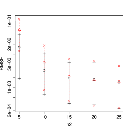
Figure 1: Comparison between kriging and co-kriging with $n_{1}=25$ runs for the cheap code (500 nested design sets have been randomly generated for each $n_{2}$). The circles represent the averaged RMSE of the co-kriging, the triangles represent the averaged RMSE of the kriging, the crosses represent the quantiles of probability 5% and 95% for the co-kriging RMSE and the times signs represent the quantiles of probability 5% and 95% of the kriging RMSE. Co-kriging predictions are better than the ordinary kriging ones for small $n_{2}$ and they converge to the same accuracy when $n_{2}$ tends to $n_{1}=25$.

In Figure 1, we can see that the errors converge to the same value when $n_{2}$ tends to $n_{1}$. Indeed, due to the Markov property given in Section 2.1, when $D_{2}=D_{1}$, only the observations $z_{2}$ are taken into account. Furthermore, we can see that for small values of $n_{2}$, it is worth considering the co-kriging model since its accuracy is significantly better than the one of the kriging model.

5.3 Nested space filling design

As presented in Section 2 we consider nested experimental design sets: $\forall t=2,\dots,s\quad D_{t}\subseteq D_{t-1}$. Therefore, we have to adopt particular design strategies to uniformly spread the inputs for all $D_{t}$. A strategy based on Orthogonal array-based Latin hypercube for nested space-filling designs is proposed by [Qian et al., 2009].
We consider here another strategy for space-filling design, described in the following algorithm, which is very simple and not time-consuming. The number of points $n_{t}$ for each design $D_{t}$ is prescribed by the user, as well as the experimental design method applied to determine the coarsest grid $D_{s}$ used for the most expensive code $z_{s}$ (see [Fang et al., 2006] for a review of different methods).

ALGORITHM

• build $D_{s}=\{x_{j}^{(s)}\}_{j=1,\dots,n_{s}}$ with the experimental design method prescribed by the user.

• for $t$ = $s$ to $2$ do:

  • build design $\tilde{D}_{t-1}$ with the experimental design method prescribed by the user.

  • for $i$ = $1$ to $n_{t}$ do:

    • find $\tilde{x}_{j}^{(t-1)}\in\tilde{D}_{t-1}$ the closest point from $x_{i}^{(t)}\in D_{t}$ where $j\in[1,n_{t-1}]$.

    • remove $\tilde{x}_{j}^{(t-1)}$ from $\tilde{D}_{t-1}$.

  • end for

  • $D_{t-1}=\tilde{D}_{t-1}\cup D_{t}$.

• end for

This strategy allows us to use any space-filling design method and it conserves the initial structure of the experimental design $D_{s}$ of the most accurate code, contrarily to a strategy based on selection of subsets of an experimental design for the less accurate code as presented by [Kennedy and O’Hagan, 2000] and [Forrester et al., 2007]. We hence can ensure that $D_{s}$ has excellent space-filling properties. Moreover, the experimental design $D_{t-1}$ being equal to $\tilde{D}_{t-1}\cup D_{t}$, this method ensure the nested property.

In the presented application, we consider $n_{2}=5$ points for the expensive code $z_{2}(x)$ and $n_{1}=25$ points for the cheap one $z_{1}(x)$. We apply the previous algorithm to build $D_{2}$ and $D_{1}$ such that $D_{2}\subset D_{1}$. For the experimental design set $D_{2}$, we use a Latin-Hypercube-Sampling [Stein, 1987] optimized with respect to the S-optimality criterion which maximizes the mean distance from each design point to all the other points [Stocki, 2005]. Furthermore, the set $D_{1}$ is built using a maximum entropy design [Shewry and Wynn, 1987] optimized with the Fedorov-Mitchell exchange algorithm [Currin et al., 1991]. These algorithms are implemented in the library R lhs. The obtained nested designs are shown in Figure 2.

Figure 2: Nested experimental design sets for the hydrodynamic application. The crosses represent the $n_{1}=25$ points of the experimental design set $D_{1}$ of the cheap code and the circles represent the $n_{2}=5$ points of the experimental design set $D_{2}$ of the expensive code.

5.4 Multi-fidelity surrogate model for the dissipation factor $eps$

We build here a co-kriging model for the dissipation factor $eps$. The obtained model is compared to a kriging one. This first example is used to illustrate the efficiency of the co-kriging method compared to the kriging. It will also allow us to highlight the difference between the simple and the universal co-kriging.

We use the experimental design sets presented in Section 5.3. To validate and compare our models, the 175 simulations of the complex code uniformly spread on $[0.5,1.5]\times[1.5,2.3]$ are used. To build the different correlation matrices, we consider a tensorised matern-$\frac{5}{2}$ kernel (see [Rasmussen and Williams, 2006]):

$$r(x,x^{\prime};\theta_{t})=r_{1d}(x_{1},x_{1}^{\prime};\theta_{t,1})r_{1d}(x_{2},x_{2}^{\prime};\theta_{t,2})$$ (25)

with $x=(x_{1},x_{2})\in[0.5,1.5]\times[1.5,2.3]$, $\theta_{t,1},\theta_{t,2}\in(0,+\infty)$ and:

$$r_{1d}(x_{i},x_{i}^{\prime};\theta_{t,i})=\left(1+\sqrt{5}\frac{|x_{i}-x_{i}^{\prime}|}{\theta_{t,i}}+\frac{5}{3}\frac{(x_{i}-x_{i}^{\prime})^{2}}{\theta_{t,i}^{2}}\right)\mathrm{exp}\left(-\sqrt{5}\frac{|x_{i}-x_{i}^{\prime}|}{\theta_{t,i}}\right)$$ (26)

Then, we consider $g_{1}(x)=1$, $f_{2}(x)=1$, $f_{1}(x)=1$ (see Section 2.1 and 2.2) and, using the concentrated maximum likelihood (see Section 5.1), we have the following estimations for the correlation hyper-parameters: $\hat{\theta}_{1}=(0.69,1.20)$ and $\hat{\theta}_{2}=(0.27,1.37)$.

According to the values of the hyper-parameter estimates, the co-kriging model is smooth since the correlation lengths are of the same order as the size of the input parameter space. Furthermore, the estimated correlation between the two codes is $82.64\%$, which shows that the amount of information contained in the cheap code is substantial.

Table 1 presents the results of the parameter estimations (see Section 2.4).

Trend coefficient	$\Sigma_{t}\nu_{t}$	$\Sigma_{t}/\sigma_{t}^{2}$
$\beta_{1}$	$8.84$	$0.48$
$\left(\begin{array}[]{c}\beta_{\rho_{1}}\\ \beta_{2}\\ \end{array}\right)$	$\left(\begin{array}[]{c}0.92\\ 0.74\\ \end{array}\right)$	$\left(\begin{array}[]{cc}1.98&-18.13\\ -18.13&165.82\\ \end{array}\right)$
Variance coefficient	$Q_{t}$	$2\alpha_{t}$
$\sigma_{1}^{2}$	$6.98$	$24$
$\sigma_{2}^{2}$	$0.06$	$3$

Table 1: Application: hydrodynamic simulator. Parameter estimation results for the response $eps$ (see equations (14) and (16)).

We see in Table 1 that the correlation between $\beta_{\rho_{1}}$ and $\beta_{2}$ is important which highlights the importance of taking into account the correlation between these two coefficients for the parameter estimation. We also see that the adjustment parameter $\beta_{\rho_{1}}$ is close to 1, which means that the two codes are highly correlated.

Figure 3 illustrates the contour plot of the kriging and co-kriging means, we can see significant differences between the two surrogate models.

Figure 3: Contour plot of the kriging mean (left picture) and the co-kriging mean (right picture). The triangles represent the $n_{2}=5$ points of the experimental design set of the expensive code.

Table 2 compares the prediction accuracy of the co-kriging and the kriging models. The different coefficients are estimated with the 175 responses of the complex code on the test set:

• MaxAE: Maximal absolute value of the observed error.

• RMSE : Root mean squared value of the observed error.

• $Q_{2}=1-||\mu_{Z_{2}}(D_{\mathrm{test}})-z_{2}(D_{\mathrm{test}})||^{2}/||\mu_{Z_{2}}(D_{\mathrm{test}})-\bar{z}_{2}||^{2}$, with $\bar{z}_{2}=(\sum_{i=1}^{n_{2}}z_{2}(x_{i}^{\mathrm{test}}))/n_{2}$.

• RIMSE : Root of the average value of the kriging or co-kriging variance.

	$Q_{2}$	RMSE	MaxAE	RIMSE.
kriging	75.83%	0.133	0.49	0.110
co-kriging	98.01%	0.038	0.14	0.046

Table 2: Application: hydrodynamic simulator. Comparison between kriging and co-kriging. The co-kriging model provides predictions significantly better than the ones of the kriging model.

We can see that the difference of accuracy between the two models is important. Indeed, the one of the co-kriging model is significantly better. Furthermore, comparing the RMSE and the RIMSE estimations in Table 2, we see that we have a good estimation of the predictive distribution variances for the two models. We note that the predictive variance for the co-kriging is obtained with a simple co-kriging model. Therefore, it will be slightly larger in the universal co-kriging case. Indeed, by computing the universal co-kriging equations, we find $\mathrm{RIMSE}=0.058$.

We can compare the RMSE obtained with the test set with the RMSE obtained with a Leave-One-Out cross validation procedure (see Section 4). For this procedure, we test our model on $n_{2}=5$ validation sets obtained by removing one observation at a time. As presented in Section 4, we can either choose to remove the observations from $z_{2}$ or from $z_{2}$ and $z_{1}$. The root mean squared error of the Leave-One-Out cross validation procedure obtained by removing observations from $z_{2}$ is RMSE${}_{z_{2},LOO}=4.80.10^{-3}$ whereas the one obtained by removing observations from $z_{2}$ and $z_{1}$ is RMSE${}_{z_{1},z_{2},LOO}=0.10$. Comparing RMSE${}_{z_{2},LOO}$ and RMSE${}_{z_{1},z_{2},LOO}$ to the RMSE obtained with the external test set, we see that the procedure which consists in removing points from $z_{2}$ and $z_{1}$ provides a better proxy for the generalization error. Indeed, RMSE${}_{z_{2},LOO}$ is a relevant proxy for the generalization error only at points where $z_{1}$ is available. Therefore, it underestimates the error at locations where $z_{1}$ is unknown.

Figure 4 represents the mean and confidence intervals at plus or minus twice the standard deviation of the simple and universal co-krigings for points along the vertical line $x_{1}=0.99$ and the horizontal line $x_{2}=1.91$ ($x=(0.99,1.91)$ corresponds to the coordinates of the point of $D_{2}$ in the center of the domain $[0.5,1.5]\times[1.5,2.3]$ in Figure 2). In Figure 4 on the right hand side, we see a necked point around the coordinates $x_{1}=1.5$ since, in the direction of $x_{2}$, the correlation hyper-parameters length for $Z_{1}(x)$ and $\delta_{2}(x)$ are large ($\theta_{1,2}=1.20$ and $\theta_{2,2}=1.37$) and a point of $D_{2}$ has almost the same coordinate.

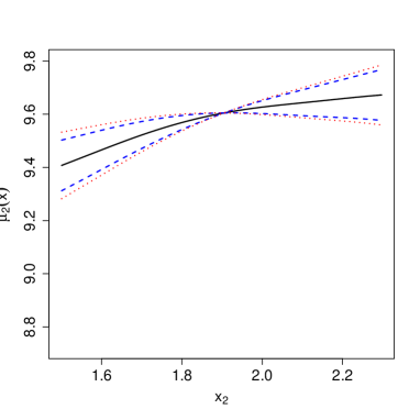
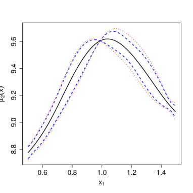
Figure 4: Mean and confidence intervals for the simple and the universal co-kriging. The figure on the left hand side represents the predictions along the vertical line $x_{1}=0.99$ and the figure on the right hand side represents the predictions along the horizontal line $x_{2}=1.91$. The solid black lines represent the mean of the two co-kriging models, the dashed lines represent the confidence interval at plus or minus twice the standard deviation of the simple co-kriging and the dotted lines represent the same confidence intervals for the universal co-kriging.

5.5 Multi-fidelity surrogate model for the mixture characteristic length $L_{c}$

In this section, we build a co-kriging model for the mixture characteristic length $L_{c}$. The aim of this example is to highlight that it can be worth having an adjustment coefficient $\rho_{1}$ depending on $x$. We use the same training and test sets as in the previous section and we consider a tensorised matern-$\frac{5}{2}$ kernel (25). Let us consider the two following cases:

• Case 1: $g_{1}(x)=1$, $f_{2}(x)=1$ and $f_{1}(x)=1$

• Case 2: $g_{1}^{T}(x)=(\begin{array}[]{cc}1&x_{1}\end{array})$, $f_{2}(x)=1$ and $f_{1}(x)=1$

We have the following hyper-parameter maximum likelihood estimates for the two cases

• Case 1: $\hat{\theta}_{1}=(0.52,1.09)$ and $\hat{\theta}_{2}=(0.03,0.02)$

• Case 2: $\hat{\theta}_{1}=(0.52,1.09)$ and $\hat{\theta}_{2}=(0.14,1.37)$

The estimation of $\hat{\theta}_{1}$ is identical in the two cases since it does not depend on $\rho_{1}$ and it is estimated with the same observations. Furthermore, we can see an important difference between the estimates of $\hat{\theta}_{2}$. Indeed, they are larger in the Case 2 than in the Case 1 which indicates that the model is smoother in the Case 2. Table 3 presents the estimations of $\beta_{1}$ and $\sigma_{1}^{2}$ for the two cases (see Section 2.4).

Trend coefficient	$\Sigma_{1}\nu_{1}$	$\Sigma_{1}/\sigma_{1}^{2}$
$\beta_{1}$	$1.26$	$0.97$
Variance coefficient	$Q_{1}$	$2\alpha_{1}$
$\sigma_{1}^{2}$	$15.62$	$24$

Table 3: Application: hydrodynamic simulator. Estimations of $\beta_{1}$ and $\sigma_{1}^{2}$ for the response $L_{c}$ (see equations (14) and (16)).

Then, Table 4 presents the estimations of $\beta_{2}$, $\beta_{\rho_{1}}$ and $\sigma_{2}^{2}$ for the Case 1, i.e. when $\rho_{1}$ is constant (see Section 2.4).

Trend coefficient	$\Sigma_{2}\nu_{2}$	$\Sigma_{2}/\sigma_{2}^{2}$
$\left(\begin{array}[]{c}\beta_{\rho_{1}}\\ \beta_{2}\\ \end{array}\right)$	$\left(\begin{array}[]{c}1.49\\ -0.26\\ \end{array}\right)$	$\left(\begin{array}[]{cc}0.83&-0.79\\ -0.79&0.95\\ \end{array}\right)$
Variance coefficient	$Q_{2}$	$2\alpha_{2}$
$\sigma_{2}^{2}$	$0.01$	$3$

Table 4: Application: hydrodynamic simulator. Estimations of $\beta_{2}$, $\beta_{\rho_{1}}$ and $\sigma_{2}^{2}$ for the Case 1, i.e. when $\rho_{1}$ is constant, for the response $L_{c}$ (see equations (14) and (16)).

Finally, Table 5 presents the estimations of $\beta_{2}$, $\beta_{\rho_{1}}$ and $\sigma_{2}^{2}$ for the Case 2, i.e. when $\rho_{1}$ depends on $x$ (see Section 2.4).

Trend coefficient	$\Sigma_{2}\nu_{2}$	$\Sigma_{2}/\sigma_{2}^{2}$
$\left(\begin{array}[]{c}\beta_{\rho_{1}}\\ \beta_{2}\\ \end{array}\right)$	$\left(\begin{array}[]{c}1.66\\ -0.48\\ -0.04\\ \end{array}\right)$	$\left(\begin{array}[]{ccc}2.34&-3.50&0.44\\ -3.50&9.18&-3.67\\ 0.44&-3.67&2.60\end{array}\right)$
Variance coefficient	$Q_{2}$	$2\alpha_{2}$
$\sigma_{2}^{2}$	$3.24.10^{-4}$	$2$

Table 5: Application: hydrodynamic simulator. Estimations of $\beta_{2}$, $\beta_{\rho_{1}}$ and $\sigma_{2}^{2}$ for the Case 2, i.e. when $\rho_{1}$ depends on $x$, for the response $L_{c}$ (see equations (14) and (16)).

We see in Table 4 that the adjustment coefficient is around 1.5 which indicates that the magnitude of the expensive code is slightly more important than the one of the cheap code. Furthermore, we see in Table 5 that if we consider an adjustment coefficient which linearly depends on $x_{1}$ (i.e. with $g_{1}^{T}(x)=(\begin{array}[]{cc}1&x_{1}\end{array})$), the constant part of $\beta_{\rho_{1}}$ is more important (it is around 1.66) and there is a negative slope in the direction $x_{1}$ (it is around $-0.48$). Since $x\in[0.5,1.5]$, the averaged value of $\rho_{1}$ is 1.18 and goes from 1.42 at $x_{1}=0.5$ to 0.94 at $x_{1}=1.5$. We see also a significant difference between the two case for the variance estimation. Indeed, the variance estimate in the Case 1 (see Table 4) is much more important than the one in the Case 2 (see Table 5). This could mean that we learn better in the Case 2 than in the Case 1.

Figure 5 illustrates the contour plot of the two co-kriging models, i.e. when $\rho_{1}$ is constant and when $\rho_{1}$ depends on $x$.

Figure 5: Contour plot of the co-kriging mean when $\rho_{1}$ is constant (on the left hand side) and when $\rho_{1}$ is depends on $x$ (of the right hand side). The triangles represent the $n_{2}=5$ points of the experimental design set of the expensive code.

Furthermore, Table 6 compares the prediction accuracy of the co-kriging in the two cases. The precision is computed on the test set of 175 observations.

	RMSE	MaxAE
Case 1	$7.26.10^{-3}$	0.23
Case 2	$1.53.10^{-3}$	0.16

Table 6: Application: hydrodynamic simulator. Comparison between co-kriging when $\rho_{1}$ is constant (Case 1) and co-kriging when $\rho_{1}$ depends on $x$ (Case 2). The Case 2 provides predictions better than the Case 1, it is hence worthwhile to consider an adjustment coefficient that is not constant.

We see that the co-kriging model in Case 2 is clearly better than the one in Case 1. Therefore, we illustrate in this application that it can be worth considering an adjustment coefficient not constant contrarily to the model presented in [Kennedy and O’Hagan, 2000] and [Forrester et al., 2007].

6 Conclusion

We have presented in this paper a recursive formulation for a multi-fidelity co-kriging model. This model allows us to build surrogate models using data from simulations of different levels of fidelity.

The strength of the suggested approach is that it considerably reduces the complexity of the co-kriging model while it preserves its predictive efficiency. Furthermore, one of the most important consequences of the recursive formulation is that the construction of the surrogate model is equivalent to build $s$ independent krigings. Consequently, we can naturally adapt results of kriging to the proposed co-kriging model.

First, we present a Bayesian estimation of the model parameters which provides closed form expressions for the parameters of the posterior distributions. We note that, from these posterior distributions, we can deduce the maximum likelihood estimates of the parameters. Second, thanks to the joint distributions of the parameters and the recursive formulation, we can deduce closed form formulas for the mean and covariance of the posterior predictive distribution. Due to their similarities with the universal kriging equations, we call these formulas the universal co-kriging equations. Third, we present closed form expressions for the cross-validation equations of the co-kriging surrogate model. These expressions reduce considerably the complexity of the cross-validation procedure and are derived from the one of kriging model that we have extended.

The suggested model has been successfully applied to a hydrodynamic code. We also present in this application a practical way to design the experiments of the multi-fidelity model.

7 Acknowledgements

The authors thank Dr. Claire Cannamela for providing the data for the application and for interesting discussions.

Appendix A Proofs

A.1 Proof of Proposition 1

Let us consider the co-kriging mean of the model (1) presented in [Kennedy and O’Hagan, 2000] for a $t$-level co-kriging with $t=2,\dots,s$:

$$m_{Z_{t}}(x)=h_{t}(x)^{T}\beta^{(t)}+t_{t}(x)^{T}V_{t}^{-1}(z^{(t)}-H_{t}\beta^{(t)})$$

where $\beta^{(t)}=(\beta_{1}^{T},\dots,\beta_{t}^{T})^{T}$, $z^{(t)}=(z_{1}^{T},\dots,z_{t}^{T})^{T}$ and $h_{t}(x)^{T}$ is defined in the following equation:

$$h_{t}(x)^{T}=\left(\left(\prod_{i=1}^{t-1}{\rho_{i}(x)}\right)f_{1}^{T}(x),\left(\prod_{i=2}^{t-1}{\rho_{i}(x)}\right)f_{2}^{T}(x),\dots,\rho_{t-1}(x)f_{t-1}^{T}(x),f_{t}^{T}(x)\right)$$ (27)

We have:

$$h_{t}(x)^{T}\beta^{(t)} = \rho_{t-1}(x)\left(\left(\prod_{i=1}^{t-2}{\rho_{i}(x)}\right)f_{1}^{T}(x),\left(\prod_{i=2}^{t-2}{\rho_{i}(x)}\right)f_{2}^{T}(x),\dots,f_{t-1}^{T}(x)\right)\beta^{(t-1)}+f_{t}^{T}(x)\beta_{t}$$

$$= \rho_{t-1}(x)h_{t-1}(x)^{T}\beta^{(t-1)}+f_{t}^{T}(x)\beta_{t}$$

Then, from equations:

$$\mathrm{cov}(Z_{t}(x),Z_{t^{\prime}}(x^{\prime})|\sigma^{2},\beta,\beta_{\rho})=\left(\prod_{i=t^{\prime}}^{t-1}\rho_{i}(x)\right)\mathrm{cov}(Z_{t^{\prime}}(x),Z_{t^{\prime}}(x^{\prime})|\sigma^{2},\beta,\beta_{\rho})$$ (28)

and:

$$\mathrm{cov}(Z_{t}(x),Z_{t}(x^{\prime})|\sigma^{2},\beta,\beta_{\rho})=\sum_{j=1}^{t}{\sigma_{j}^{2}\left(\prod_{i=j}^{t-1}{\rho_{i}(x)\rho_{i}(x^{\prime})}\right)r_{j}(x,x^{\prime})}$$ (29)

with $t>t^{\prime}$ , we have the following equality:

$$t_{t}(x)^{T}V_{t}^{-1}z^{(t)} = \rho_{t-1}(x)t_{t-1}(x)^{T}V_{t-1}^{-1}z^{(t-1)}-\left(\rho_{t-1}^{T}(D_{t})\right)\odot\left(r_{t}^{T}(x)R_{t}^{-1}z_{t-1}(D_{t})\right)$$

$$+r_{t}^{T}(x)R_{t}^{-1}z_{t}$$

and with equation (6):

$$t_{t}(x)^{T}V_{t}^{-1}H_{t}\beta^{(t)}=\rho_{t-1}(x)t_{t-1}(x)^{T}V_{t-1}^{-1}H_{t-1}\beta^{(t-1)}+r_{t}^{T}(x)R_{t}^{-1}F_{t}(D_{t})\beta_{t}$$

where $\odot$ stands for the element by element matrix product. We hence obtain the recursive relation:

$$m_{Z_{t}}(x)=\rho_{t-1}(x)m_{Z_{t-1}}(x)+f_{t}^{T}(x)\beta_{t}+r_{t}^{T}(x)R_{t}^{-1}\left[z_{t}-\rho_{t-1}(D_{t})\odot z_{t-1}(D_{t})-F_{t}(D_{t})\beta_{t}\right]$$

The co-kriging mean of the model (9) satisfies the same recursive relation (6), and we have $m_{Z_{1}}(x)=\mu_{Z_{1}}(x)$. This proves the first equality of Proposition 1:

$$\mu_{Z_{s}}(x)=m_{Z_{s}}(x)$$

We follow the same guideline for the co-kriging covariance:

$$s^{2}_{Z_{t}}(x,x^{\prime})=v^{2}_{Z_{t}}(x,x^{\prime})-t_{t}^{T}(x)V_{t}^{-1}t_{t}(x^{\prime})$$

where $v^{2}_{Z_{t}}(x,x^{\prime})$ is the covariance between $Z_{t}(x)$ and $Z_{t}(x^{\prime})$ and $s^{2}_{Z_{t}}(x,x^{\prime})$ is the covariance function of the conditioned Gaussian process $[Z_{t}(x)|\mathcal{Z}^{(t)}=z^{(t)},\beta,\beta_{\rho},\sigma^{2}]$ for the model (1). From equation (8), we can deduce the following equality:

$$\sigma^{2}_{Z_{t}}(x,x^{\prime})=\rho_{t-1}(x)\rho_{t-1}(x^{\prime})v^{2}_{Z_{t-1}}(x,x^{\prime})+v_{t}^{2}(x,x^{\prime})$$

where $\sigma^{2}_{Z_{t}}(x,x^{\prime})$ is the covariance function of the conditioned Gaussian process $[Z_{t}(x)|\mathcal{Z}^{(t)}=z^{(t)},\beta_{t},\beta_{\rho_{t-1}},\sigma_{t}^{2}]$ of the recursive model (9). Then, from equation (7) and (8), we have:

$$t_{t}^{T}(x)V_{t}^{-1}t_{t}(x^{\prime})=\rho_{t-1}(x)\rho_{t-1}(x^{\prime})t_{t-1}^{T}(x)V_{t-1}^{-1}t_{t-1}(x^{\prime})+\sigma_{t}^{2}r_{t}^{T}(x)R_{t}^{-1}r_{t}(x^{\prime})$$

Finally we can deduce the following equality:

$$s^{2}_{Z_{t}}(x,x^{\prime})=\rho_{t-1}(x)\rho_{t-1}(x^{\prime})\left(v^{2}_{Z_{t-1}}(x,x^{\prime})-t_{t-1}^{T}(x)V_{t-1}^{-1}t_{t-1}(x^{\prime})\right)+\sigma_{t}^{2}\left(1-r_{t}^{T}(x)R_{t}^{-1}r_{t}(x^{\prime})\right)$$

which is equivalent to:

$$s^{2}_{Z_{t}}(x,x^{\prime})=\rho_{t-1}(x)\rho_{t-1}(x^{\prime})s^{2}_{Z_{t-1}}(x,x^{\prime})+\sigma_{t}^{2}\left(1-r_{t}^{T}(x)R_{t}^{-1}r_{t}(x^{\prime})\right)$$

This is the same recursive relation as the one satisfies by the co-kriging covariance $\sigma_{Z_{t}}^{2}(x,x^{\prime})$ of the model (9) (see equation (12)). Since $s^{2}_{Z_{1}}(x,x^{\prime})=\sigma^{2}_{Z_{1}}(x,x^{\prime})$, we have :

$$\sigma_{Z_{s}}^{2}(x,x^{\prime})=s_{Z_{s}}^{2}(x,x^{\prime})$$

This equality with $x=x^{\prime}$ proves the second equality of Proposition 1. $\Box$

A.2 Proof of Proposition 2

Noting that the mean of the predictive distribution in equation (10) does not depend on $\sigma_{t}^{2}$ and thanks to the law of total expectation, we have the following equality:

$$\mathbb{E}\left[Z_{t}(x)|\mathcal{Z}^{(t)}=z^{(t)}\right]=\mathbb{E}\left[\mathbb{E}\left[Z_{t}(x)|\mathcal{Z}^{(t)}=z^{(t)},\sigma^{2}_{t},\beta_{t},\beta_{\rho_{t-1}}\right]\left|\mathcal{Z}^{(t)}=z^{(t)}\right.\right]$$

From the equations (11) and (14), we directly deduce the equation (17). Then, we have the following equality:

$$\mathrm{var}\left(\mu_{Z_{t}}(x)\left|z^{(t)},\sigma_{t}^{2}\right.\right)=(h_{t}^{T}(x)-r_{t}(x)^{T}R_{t}^{-1}H_{t})\Sigma_{t}(h_{t}^{T}(x)-r_{t}(x)^{T}R_{t}^{-1}H_{t})^{T}$$ (30)

The law of total variance states that:

$$\mathrm{var}(Z_{t}(x)|z^{(t)},\sigma_{t}^{2}) = \mathbb{E}\left[\mathrm{var}(Z_{t}(x)|z^{(t)},\beta_{t},\beta_{\rho_{t-1}},\sigma_{t}^{2})\left|z^{(t)},\sigma_{t}^{2}\right.\right]$$

$$+ \mathrm{var}\left(\mathbb{E}\left[Z_{t}(x)|z^{(t)},\beta_{t},\beta_{\rho_{t-1}},\sigma_{t}^{2}\right]\left|z^{(t)},\sigma_{t}^{2}\right.\right)$$

Thus, from equations (11), (17) and (30), we obtain:

$$\begin{array}[]{lll}\mathrm{var}(Z_{t}(x)|\mathcal{Z}^{(t)}=z^{(t)},\sigma_{t}^{2})&=&\hat{\rho}_{t}^{2}(x)\mathrm{var}(Z_{t-1}(x)|\mathcal{Z}^{(t-1)}=z^{(t-1)},\sigma_{t}^{2})+\sigma_{t}^{2}\left(1-r_{t}^{T}(x)R_{t}^{-1}r_{t}^{T}(x)\right)\\ &&+\left(h_{t}^{T}-r_{t}^{T}(x)R_{t}^{-1}H_{t}\right)\Sigma_{t}\left(h_{t}^{T}-r_{t}^{T}(x)R_{t}^{-1}H_{t}\right)^{T}\\ \end{array}$$ (31)

Again using the law of total variance and the independence between $\mathbb{E}\left[Z_{t}(x)|\mathcal{Z}^{(t)}=z^{(t)},\beta_{t},\beta_{\rho_{t-1}}\right]$ and $\sigma_{t}^{2}$, we have:

$$\mathrm{var}(Z_{t}(x)|z^{(t)})=\mathbb{E}\left[\mathrm{var}(Z_{t}(x))|z^{(t)},\sigma_{t}^{2}\right]$$ (32)

We obtain the equation (18) from equation (16) by noting that the mean of an inverse Gamma distribution $\mathcal{IG}(a,b)$ is $b/(a-1)$. $\Box$

A.3 Proof of Proposition 3

Let us consider that $\xi_{s}$ is the index of the $k$ last points of $D_{s}$. We denote by $D_{\mathrm{test}}$ these points. First we consider the variance and the trend parameters as fixed, i.e. $\sigma_{t,-\xi_{t}}^{2}=\frac{Q_{t}}{2(a_{t}-1)}$ and $\lambda_{t,-\xi_{t}}=\Sigma_{t}\nu_{t}$, and $\mathcal{V}_{s}=0$, i.e. we are in the simple co-kriging case. Thanks to the block-wise inversion formula, we have the following equality:

$$R_{s}^{-1}=\left(\begin{array}[]{cc}A&B\\ B^{T}&\mathcal{Q}^{-1}\\ \end{array}\right)$$ (33)

with $A=\left[R_{s}^{-1}\right]_{[-\xi_{s},-\xi_{s}]}+\left[R_{s}^{-1}\right]_{[-\xi_{s},-\xi_{s}]}\left[R_{s}^{-1}\right]_{[-\xi_{s},\xi_{s}]}Q^{-1}\left[R_{s}^{-1}\right]_{[\xi_{s},-\xi_{s}]}\left[R_{s}^{-1}\right]_{[-\xi_{s},-\xi_{s}]}$,
$B=-\left[R_{s}^{-1}\right]_{[-\xi_{s},-\xi_{s}]}\left[R_{s}^{-1}\right]_{[-\xi_{s},\xi_{s}]}\mathcal{Q}^{-1}$ and:

$$\mathcal{Q}=\left[R_{s}^{-1}\right]_{[\xi_{s},\xi_{s}]}-\left[R_{s}^{-1}\right]_{[\xi_{s},-\xi_{s}]}\left(\left[R_{s}^{-1}\right]_{[-\xi_{s},-\xi_{s}]}\right)^{-1}\left[R_{s}^{-1}\right]_{[-\xi_{s},\xi_{s}]}$$ (34)

We note that $\frac{Q_{s}}{2(a_{s}-1)}\mathcal{Q}=\frac{Q_{t}}{2(a_{t}-1)}\left(\left[R_{s}^{-1}\right]_{[\xi_{s},\xi_{s}]}\right)^{-1}$ represents the covariance matrix of the points in $D_{\mathrm{test}}$ with respect to the covariance kernel of a Gaussian process of kernel $\frac{Q_{s}}{2(a_{s}-1)}r_{s}(x,x^{\prime})$ (which is the one of $\delta_{s}(x)$) conditioned by the points $D_{s}\setminus D_{\mathrm{test}}$. Therefore, from the previous remark and the equation (12), we can deduce the equation (21).

Furthermore, we have the following equality:

$$\begin{array}[]{lll}\left(\left[R_{s}^{-1}\right]_{[\xi_{s},\xi_{s}]}\right)^{-1}\left[R_{s}^{-1}\left(z_{s}-H_{s}\lambda_{s,-\xi_{s}}\right)\right]_{[\xi_{s}]}&=&z_{s}(D_{\mathrm{test}})-h_{s}^{T}(D_{\mathrm{test}})\Sigma_{s}\nu_{s}\\ &-&\left[R_{s}^{-1}\right]_{[-\xi_{s},\xi_{s}]}\left(\left[R_{s}^{-1}\right]_{[\xi_{s},\xi_{s}]}\right)^{-1}\\ &\times&\left(z_{s-1}(D_{s}\setminus D_{\mathrm{test}})-[H_{s}^{T}]_{[-\xi_{s}]}\Sigma_{s}\nu_{s}\right)\end{array}$$ (35)

From this equation and equation (11), we can directly deduce the equation (19) with $\varepsilon_{Z_{s},\xi_{s}}=z_{s}(D_{\mathrm{test}})-\mu_{Z_{s}}(D_{\mathrm{test}})$.

Then, we suppose the trend and the variance parameters as unknown and we have to re-estimate them when we remove the observations. Thanks to the parameter estimations presented in Section 2.4, we can deduce that the estimates of $\sigma_{t,-\xi_{t}}^{2}$ and $\lambda_{t,-\xi_{t}}$ when we remove observations of index $\xi_{t}$ are given by the following equations:

$$\lambda_{s,-\xi_{s}}\left([H_{s}^{T}]_{-\xi_{s}}K_{s}[H_{s}]_{-\xi_{s}}\right)=[H_{s}^{T}]_{-\xi_{s}}K_{s}z_{s}(D_{s}\setminus D_{test})$$ (36)

and:

$$\sigma_{s,-\xi_{s}}^{2}=\frac{\left(z_{s}(D_{s}\setminus D_{\mathrm{test}})-[H_{s}]_{-\xi_{s}}\lambda_{s,-\xi_{s}}\right)^{T}K_{s}\left(z_{s}(D_{s}\setminus D_{\mathrm{test}})-[H_{s}]_{-\xi_{s}}\lambda_{s,-\xi_{s}}\right)}{n_{s}-p_{s}-q_{s-1}-n_{train}}$$ (37)

with $K_{s}=\left(\left[R_{s}\right]_{[-\xi_{s},-\xi_{s}]}\right)^{-1}$.

From the equality (33), we can deduce that $K_{s}=A-B\mathcal{Q}B^{T}$ from which we obtain the equation (20). Finally, to obtain the cross-validation equations for the universal co-kriging, we just have to estimate the following quantity (see equation (18)):

$$\left(h_{s}^{T}(D_{\mathrm{test}})^{T}-\left[R_{s}^{-1}\right]_{[-\xi_{s},\xi_{s}]}K_{s}[H_{s}]_{-\xi_{s}}\right)\Sigma_{s}\left(h_{s}^{T}(D_{\mathrm{test}})^{T}-\left[R_{s}^{-1}\right]_{[-\xi_{s},\xi_{s}]}K_{s}[H_{s}]_{-\xi_{s}}\right)^{T}$$ (38)

with $\Sigma_{s}=\left([H_{s}^{T}]_{-\xi_{s}}K_{s}[H_{s}]_{-\xi_{s}}\right)^{-1}$. The following equality:

$$\left(h_{s}^{T}(D_{\mathrm{test}})^{T}-\left[R_{s}^{-1}\right]_{[-\xi_{s},\xi_{s}]}K_{s}[H_{s}]_{-\xi_{s}}\right)=\left(\left([R_{s}^{-1}]_{[\xi_{s},\xi_{s}]}\right)^{-1}\left[R_{s}^{-1}H_{s}\right]_{[\xi_{s}]}\right)$$ (39)

allows us to obtain the equation (23) and completes the proof. $\Box$

References

- [Craig et al., 1998] Craig, P. S., Goldstein, M., Seheult, A. H., and Smith, J. A. (1998). Constructing partial prior specifications for models of complex physical systems. Applied Statistics, 47:37–53.
- [Cumming and Goldstein, 2009] Cumming, J. A. and Goldstein, M. (2009). Small sample bayesian designs for complex high-dimensional models based on information gained using fast approximations. Technometrics, 51:377–388.
- [Currin et al., 1991] Currin, C., Mitchell, T., Morris, M., and Ylvisaker, D. (1991). Bayesian prediction of deterministic functions with applications to the design and analysis of computer experiments. Journal of the American Statistical Association, 86:953–963.
- [Dubrule, 1983] Dubrule, O. (1983). Cross validation of kriging in a unique neighborhood. Mathematical Geology, 15:687–699.
- [Fang et al., 2006] Fang, K.-T., Li, R., and Sudjianto, A. (2006). Design and Modeling for Computer Experiments. Chapman & Hall - Computer Science and Data Analysis Series, London.
- [Forrester et al., 2007] Forrester, A. I. J., Sobester, A., and Keane, A. J. (2007). Multi-fidelity optimization via surrogate modelling. Proc. R. Soc. A, 463:3251–3269.
- [Goldstein and Wooff, 2007] Goldstein, M. and Wooff, D. A. (2007). Bayes Linear Statistics: Theory and Methods. Chichester, England: Wiley.
- [Grégoire et al., 2005] Grégoire, O., Souffland, D., and Serge, G. (2005). A second order turbulence model for gaseous mixtures induced by Richtmyer-Meshkov instability. Journal of Turbulence, 6:1–20.
- [Higdon et al., 2004] Higdon, D., Kennedy, M., Cavendish, J. C., Cafeo, J. A., and Ryne, R. D. (2004). Combining field data and computer simulation for calibration and prediction. SIAM Journal on Scientific Computing, 26:448–466.
- [Jeffreys, 1961] Jeffreys, H. (1961). Theory of Probability. Oxford University Press, London.
- [Kennedy and O’Hagan, 2000] Kennedy, M. C. and O’Hagan, A. (2000). Predicting the output from a complex computer code when fast approximations are available. Biometrika, 87:1–13.
- [Krige, 1951] Krige, D. G. (1951). A statistical approach to some basic mine valuation problems on the witwatersrand. Technometrics, 52:119–139.
- [Patterson and Thompson, 1971] Patterson, H. and Thompson (1971). Recovery of interblock information when block sizes are unequal. Biometrika, 58:545–554.
- [Qian et al., 2009] Qian, P. Z. G., Ai, M., and Wu, C. F. J. (2009). Construction of nested space-filling designs. The Annals of Statistics, 37:3616–3643.
- [Qian and Wu, 2008] Qian, P. Z. G. and Wu, C. F. J. (2008). Bayesian hierarchical modeling for integrating low-accuracy and high-accuracy experiments. Technometrics, 50:192–204.
- [Rasmussen and Williams, 2006] Rasmussen, C. E. and Williams, C. K. I. (2006). Gaussian Processes for Machine Learning. MIT Press, Cambridge.
- [Sacks et al., 1989] Sacks, J., Welch, W. J., Mitchell, T. J., and Wynn, H. P. (1989). Design and analysis of computer experiments. Statistical Science, 4:409–423.
- [Santner et al., 2003] Santner, T. J., Williams, B. J., and Notz, W. I. (2003). The Design and Analysis of Computer Experiments. Springer, New York.
- [Shewry and Wynn, 1987] Shewry, M. C. and Wynn, H. P. (1987). Maximum entropy sampling. Journal of Applied Statistics, 14:165–170.
- [Stein, 1987] Stein, M. L. (1987). Large sample properties of simulations using latin hypercube sampling. Technometrics, 29:143–151.
- [Stein, 1999] Stein, M. L. (1999). Interpolation of Spatial Data. Springer Series in Statistics, New York.
- [Stocki, 2005] Stocki, R. (2005). A method to improve design reliability using optimal latin hypercube sampling. Computer Assisted Mechanics and Engineering Sciences, 12:87–105.
- [Zhang and Wang, 2009] Zhang, H. and Wang, Y. (2009). Kriging and cross-validation for massive spatial data. Environmetrics, 21:290–304.