Localization of an inhomogeneous Bose-Einstein condensate in a moving random potential

Abstract

We study the dynamics of a harmonically trapped quasi-one-dimensional Bose-Einstein condensate subjected to a moving disorder potential of finite extent. We show that, due to the inhomogeneity of the sample, only a percentage of the atoms is localized at supersonic velocities of a random potential. We find that this percentage can be sensitively increased by introducing suitable correlations in the disorder potential such as those provided by random dimers.

I Introduction

Suppression of wave transport in non-dissipative linear systems can be induced by the presence of disorder: the scattered waves from the modulation of the random disorder potential destructively interfere in the forward direction, with a resulting vanishing wave transmission. This phenomenon is called Anderson localization (AL) Anderson (1958, 1985). In three dimensions (3D), AL takes place for states with energy less than a threshold (mobility edge). In two (2D) and one dimensions (1D) and in the absence of interactions, all single-particle quantum states are expected to be localized Abrahams et al. (1979). However, in the presence of correlations, the situation differs and a subset of delocalized states can appear in the spectrum Dunlap et al. (1990) or an effective Tessieri (2002); Kuhl et al. (2008); Gurevich and Kenneth (2009); Lugan et al. (2009); Piraud et al. (2012) or even a true de Moura and Lyra (1998) mobility edge can be observed even at low dimensions.

Anderson localization of noninteracting atomic matter waves was observed in momentum and real space. In momentum space using kicked-rotor setups in 1D Moore et al. (1995) and 3D Chabé et al. (2008), while in real space in 1D Billy et al. (2008); Roati et al. (2008), and very recently in 3D Kondov et al. (2011); Jendrzejewski et al. (2012). On the other hand, in 2D only anomalous diffusion has been observed Robert-de Saint-Vincent et al. (2010). In the last few years it has been experimentally demonstrated that disorder strongly affects the transport properties and dynamics of a BEC, as for instance illustrated in Chen et al. (2008).

One of the outstanding challenges of physics is to understand the interplay between disorder and interactions. In the case of an interacting condensate, wave scattering from the random potential does not occur if the wave group velocity is lower than a critical velocity $v_{c}$ that coincides with the (local) sound velocity $c$ in the limit of small random potential amplitude and decreases down to vanishing values in the strong disorder limit Ianeselle et al. (2006). Thus, to observe AL in an interacting BEC it is necessary that the speed of the relative motion between the superfluid and the disorder potential is larger than $v_{c}$. This setup was proposed and theoretically studied in Refs. Paul et al. (2007, 2009); Albert et al. (2010). These authors studied the flow of an homogeneous quasi-one-dimensional Bose-Einstein condensate through a disorder potential of finite extent. That disorder potential moves with a velocity $v$ with respect to the condensate. In the subsonic regime, the flow is superfluid and the density profile is stationary. In the opposite supersonic regime, a region of stationary flow also exists, but in this case energy dissipation occurs. In this domain, depending on the extent of the disorder potential, the system is either in a Ohmic or in an AL regime, respectively characterized by a transmission decreasing linearly or exponentially with the size of the system $L$.

At variance of Refs. Paul et al. (2007, 2009); Albert et al. (2010), in this paper we study the effects of the inhomogeneity of a cigar-shaped trapped BEC in the presence of a moving disorder potential. We investigate the possibility of observing BEC localization by looking at the position of the center of mass of the condensate. If the center of mass moves along with the moving potential then the system shall be in the AL regime or in another kind of localized phase. Because of the inhomogeneity, we observe the localization of only a percentage of the atoms in the BEC. This percentage of localized atoms can be increased or suppressed by introducing ad-hoc short-range correlations on the random potential.

The paper is organized as following. In Sec. II we introduce the time-dependent nonpolynomial nonlinear Schrödinger equation (NPSE) that describes the condensate dynamics in the elongated geometry and in the presence of a moving disorder potential that we characterize by its auto-correlation function. As discussed and shown in Sec. III, the disorder potential drags the atoms with an efficiency that depends on both the scattering properties of each impurity and on the impurity density. The case of two types of impurities, single and dimerized, at different densities, have been studied, highlighting the role of correlations in the localization dynamics. Because of the inhomogeneity of the BEC, we observe that the drag force is more efficient in the BEC tails where the local sound velocity is lower and superfluidity breaks down at small drift velocities $v$. Our concluding remarks are given in Sec. IV.

II The model

II.1 Equation of motion for the BEC wavefunction

Our starting point is the equation of motion for a 3D BEC trapped into a cigar-shaped potential. Such an equation is known as the Gross-Pitaevskii equation (GPE)

$$i\hbar\frac{\partial}{\partial t}\psi(\textbf{r},t)=\left[-\frac{\hbar^{2}}{2m}\nabla^{2}+U(\textbf{r})+gN|\psi(\textbf{r},t)|^{2}\right]\psi(\textbf{r},t).$$ (1)

The wave function $\psi(\textbf{r},t)$ describes the condensate, which is constituted of $N$ atoms of mass $m$. $g=4\pi\hbar^{2}a_{s}/m$ stands for the interaction coupling constant with $a_{s}$ being the s-wave scattering length between atoms; in our system, interatomic interactions are repulsive and, as a result, $a_{s}>0$. The trapping potential $U(\textbf{r})$ is given by the sum of a static cigar-shaped harmonic trap and a time-dependent random potential:

$$U(\textbf{r},t)=\frac{1}{2}m\omega^{2}_{\perp}(x^{2}+y^{2})+\frac{1}{2}m\omega^{2}_{z}z^{2}+V(z,t)$$ (2)

with $\omega_{\perp}$ and $\omega_{z}$ the trapping frequencies in the perpendicular and longitudinal directions, respectively and $\omega_{z}\ll\omega_{\perp}$. The last time-dependent term in (2) corresponds to a random potential that is fixed in the moving frame $z^{\prime}=z-vt$, ${\bf v}=v\hat{e}_{z}$ being the drift velocity.

Under this trap geometry and a further assumption discussed below, the 3D GPE can be reduced to an effective 1D time-dependent NPSE Salasnich et al. (2002). The advantage of the 1D NPSE is that it is easier to deal with when making computations. In order to obtain such dynamical equation, we begin with a variational Ansatz

$$\psi(\textbf{r},t)=f(z,t)\phi(\textbf{r},t)=f(z,t)\frac{e^{-(x^{2}+y^{2})/2\sigma^{2}(z,t)}}{\sqrt{\pi}\sigma(z,t)}$$ (3)

where the transverse part $\phi(\textbf{r},t)$ is modeled by a Gaussian function with variance $\sigma(z,t)$. The validity of this description is based on the assumption that $\sigma(z,t)$ slowly varies as a function of $z$ and $t$ such that the kinetic energy term $\partial^{2}/\partial z^{2}$ associated to $\phi(\textbf{r},t)$ can be neglected. Both the longitudinal wave function $f(z,t)$ and the variance $\sigma(z,t)$ are determined by the energy variational principle. For $f(z,t)$ one gets the NPSE

$$\begin{split}i\hbar\frac{\partial}{\partial t}f&=\left[-\frac{\hbar^{2}}{2m}\frac{\partial^{2}}{\partial z^{2}}+\frac{1}{2}m\omega^{2}_{z}z^{2}+V(z,t)\right.\\ &\left.+\hbar\omega_{\perp}\frac{1+3a_{s}N|f|^{2}}{\sqrt{1+2a_{s}N|f|^{2}}}\right]f.\end{split}$$ (4)

The variance is given by

$$\sigma^{2}(z,t)=a^{2}_{\perp}\sqrt{1+2a_{s}N|f(z,t)|^{2}},$$ (5)

where $a_{\perp}=\sqrt{\hbar/(m\omega_{\perp})}$ is the oscillator length in the transverse direction. The 3D density profile and velocity field are then

$$\rho(\textbf{r}) =\tilde{\rho}(z)\frac{e^{-r^{2}/\sigma^{2}}}{\pi\sigma^{2}},$$ (6)

$$\textbf{v}(\textbf{r}) =v(\textbf{r})\hat{z}=\frac{\hbar}{2mi}\frac{f^{{}^{\prime}*}(z)f(z)-f^{\prime}(z)f^{*}(z)}{\tilde{\rho}}\hat{z},$$ (7)

with $\tilde{\rho}(z)=|f|^{2}$ the integrated 1D density.

The NPSE is numerically solved using a split-step method and spatial Fast Fourier transforms (FFT). First we compute the equilibrium density profile in the presence of a static disorder potential. Then, we switch on the drift velocity $v$ and compute the time evolution of the condensate wavefunction $f(z,t)$. In this work, we focus on a system of $10^{5}$ 87-Rubidium atoms subject to a transverse confinement of $\omega_{\perp}=2\pi\times 500$ Hz and a longitudinal confinement of $\omega_{z}=2\pi\times 7$ Hz. The $s$-wave scattering length has been fixed at $a_{s}=80$ Bohr radii.

II.2 The random potential

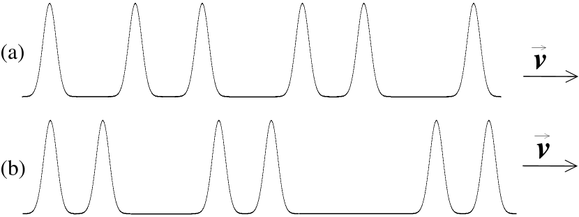
Figure 1: Schematic representation of the disorder potential. (a) The Gaussian peaks are randomly distributed (AM). (b) The peaks are distributed in a random dimer sequence (RDM).

The random potential $V(z,t)$ is modeled by the sum of $N_{\textmd{dis}}$ Gaussian functions of height $V_{\textmd{dis}}$ and width $w$, randomly distributed at positions $z_{i}=j_{i}d$, where $j_{i}$ is a random integer number and $d$ fixes the minimal distance between the peaks. Such a disorder potential could be realized by deeply trapping some impurities (heavy atoms of another species) in an optical lattice strongly detuned from the condensate atomic frequencies Gavish and Castin (2005); Vignolo et al. (2003); Schaff et al. (2010). When the disorder pattern is pulled with a constant speed $v$ through the system, if $v$ is lower than the sound speed $c=\sqrt{\mu/(2m)}$ Zaremba (1998), we expect the disorder not to affect the system because of the superfluid nature of the gas itself Paul et al. (2007). In contrast, the effect of the disorder potential should appear at $v\gtrsim c$ where the kinetic energy starts to compete with the interaction energy and the limit of a noninteracting gas is reached for $v\gg c$.

We will consider two sorts of potential patterns: (i) an Anderson-like distribution, that we will call Anderson Model (AM), where the $j_{i}$’s are randomly distributed; (ii) a Random Dimer Model (RDM) distribution where peaks are dimerized and the dimers are randomly distributed (see Fig 1). The dimers are stamped by the peak-to-peak distance $\ell$. Hereafter we consider a disorder potential characterized by an amplitude $V_{\textmd{dis}}=0.02E_{r}$, where the recoil energy $E_{r}=h^{2}/(2m\lambda^{2})$ for each atom of mass $m$ is defined with respect to the wavelength $\lambda=780$ nm, characterizing the D2 hyperfine Rubidium transition. The dimer peak-to-peak distance $\ell$ was set equal to $\lambda$ and the width of a single bump $w$ is fixed at $140\textmd{nm}$, roughly $\lambda/5$, ensuring no sizeable overlap between Gaussian functions. The disorder potentials can be characterized in term of their autocorrelation functions

$$C(|{z_{1}}-{z_{2}}|)=\langle(V({z_{1}},t)-\langle V({z_{1}},t)\rangle)(V(z_{2},t)-\langle V({z_{2}},t)\rangle)\rangle,$$ (8)

which strongly influence the nature of the energy states for low amplitude disorder near equilibrium. In the case of the AM and RDM potentials in Fig. 2 we plot the autocorrelation function for the case $d=\lambda$ and for two different peaks densities: $n_{\textmd{{dis}}}=0.12\lambda^{-1}$ (top panel) and $n_{\textmd{{dis}}}=0.5\lambda^{-1}$ (bottom panel). It is worthwhile remarking than the peak density corresponds to the average number of Gaussian peaks both in the AM and RDM potential and thus in average the number of dimers in RDM is half the number of peaks in the AM.

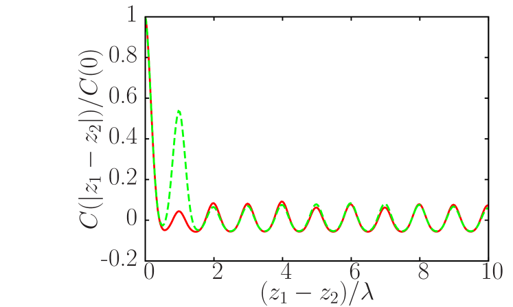
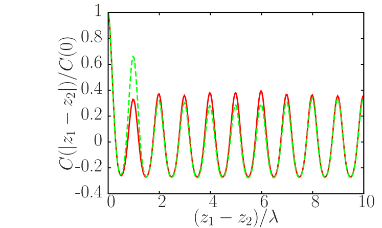
Figure 2: (Color online) Rescaled auto-correlation function $C(|{z_{1}}-{z_{2}}|)/C(0)$ as a function of $(z_{1}-z_{2})/\lambda$ for the AM (red continuous line) and RDM (green dashed line) for the case $d=\lambda$. The top panel corresponds to $n_{\textmd{{dis}}}=0.12\lambda^{-1}$, and the bottom panel to $n_{\textmd{{dis}}}=0.5\lambda^{-1}$.

The modulation with spatial period $\lambda$ for both the AM and the RDM evinces that bumps and dimers are both randomly distributed over discretized positions of step $d=\lambda$. The main difference between the AM and the RDM is that the RDM has a larger peak at $z_{1}-z_{2}=\lambda$ because of the dimer structure with $\ell=\lambda$. This is well visible at low peak density (top panel), while by increasing the bump density the probability to find dimerized structures in the AM potential increases as well. This is seen in the heights of the peaks at $z_{1}-z_{2}=j\lambda$ for the two models becoming closer even for $j=1$ (bottom panel).

In Fig. 3 we show $C(|z_{1}-z_{2}|)$ for the case $d=\lambda/2$ and $n_{\textmd{{dis}}}=0.5\lambda^{-1}$ (keeping fixed $\ell=\lambda$).

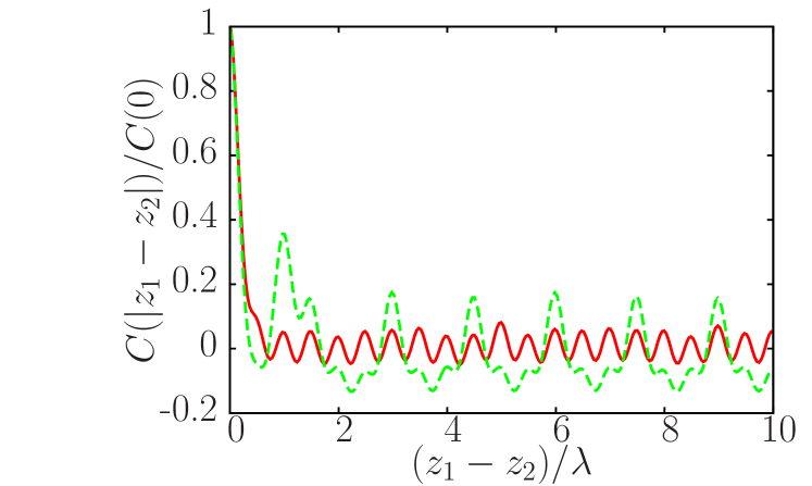
Figure 3: (Color online) Same as in Fig. 2 but for the case $d=\lambda/2$ and $n_{\textmd{{dis}}}=0.5\lambda^{-1}$.

In this case the RDM peak at $z_{1}-z_{2}=\lambda$ is lower of more than a factor 2 with respect to the case with $d=\lambda$ at the same disorder density (bottom panel of Fig. 2): we thus expect the dimer structure to play a minor role for the case $d=\lambda/2$.

III The localization fraction and the drag force

If the condensate or a part of it is localized, we expect it to follow the pulled disorder potential. The localized portion of the condensate glues to the disorder ”bandwagon” and therefore travels the same distance as the disorder potential. This dynamics depends on the forces experienced by the atoms. The force acting on the BEC center-of-mass has two terms, $F=F_{h}+F_{\textmd{dis}}$, one due to the harmonic confinement, $F_{h}=-m\omega_{z}^{2}z_{\mathrm{c.m.}}$ and the other due to the disorder potential

$$F_{\textmd{dis}}=-\int_{-\infty}^{+\infty}dz|f(z,t)|^{2}\dfrac{\partial V}{\partial z}.$$ (9)

For small center-of-mass displacements $\Delta z_{\mathrm{c.m.}}\simeq 0$, the leading term is the drag force $F_{\textmd{dis}}$ due to the disorder potential. In this regime the localization fraction $N_{loc}/N$ can be deduced by the ratio between the $\Delta z_{\mathrm{c.m.}}$ and the distance $\Delta z_{\textmd{dis}}$ traveled by the disorder potential in the same time interval, namely in this regime we can identify

$$\dfrac{N_{loc}}{N}=\dfrac{\Delta z_{\mathrm{c.m.}}}{\Delta z_{\textmd{dis}}}.$$ (10)

Indeed if the center of mass travels the same distance as the disorder potential, this would mean that the 100% of the atoms are localized. The localized condensate will stop following the moving potential and it will change direction at a time $t_{f}$ at the position $z_{f}$ verifying

$$\int_{0}^{t_{f}}F_{\textmd{dis}}(t)v_{\mathrm{c.m.}}(t){\rm d}t=\dfrac{1}{2}m\omega_{z}^{2}z_{f}^{2}.$$ (11)

Thus, the turning point $z_{f}$ will provide a direct measure of the average value of the drag force during the condensate forward motion via the relation

$$z_{f}=2\bar{F}_{\textmd{dis}}/(m\omega_{z}^{2}),$$ (12)

where we have defined

$$\bar{F}_{\textmd{dis}}=\int_{0}^{t_{f}}F_{\textmd{dis}}(t)v_{\mathrm{c.m.}}(t){\rm d}t/z_{f}=\int_{0}^{z_{f}}F_{\textmd{dis}}(t){\rm d}z_{\mathrm{c.m.}}/z_{f}.$$ (13)

The dependence of the drag force with the drift velocity gives us a direct measure of the loss of superfluidity in the system. According to the Landau criterion Landau (1941) a single impurity is expected to flow without friction below a certain velocity, corresponding to the sound velocity for a weakly interacting BEC.

III.1 The single impurities

The localization efficiency of a disorder pattern depends on the impurity density and on the reflectivity of each impurity. In this work we are comparing single impurities randomly distributed with dimerized structures. With the aim to understand the difference in behavior of the localization efficiency of a dimer with respect to a single bump, we first look at the condensate dynamics in the presence of a moving single bump (red crosses in Fig. 4) and of a moving dimer (green stars in Fig. 4).

In Fig. 4 we plot the fraction of atoms that follows the moving defect over a distance of $133\mu$m.

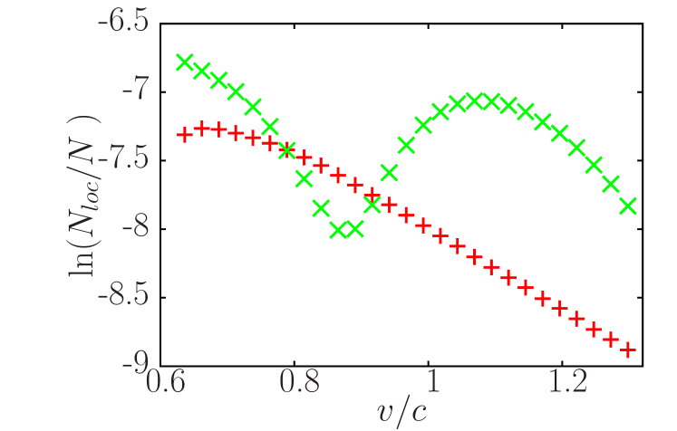
Figure 4: (Color online) Localized BEC fraction (in logarithmic scale) as a function of the disorder potential drift velocity $v$, in units of the sound speed $c$ evaluated at the center of the trap. The red crosses correspond to a single bump and the green stars to a dimer.

We observe that the localization fraction of the dimer is a strongly non-monotonic function of $v$. The single dimer localizes the atoms less efficiently than a single bump for $v\simeq 0.9c$, while it is more efficient by a factor of 3 over a velocity range of 1–1.2 $v/c$. The suppression and the enhancement of the localization are both a signature of some interference effect due to the internal structure of the single dimer. This behavior can be qualitatively reproduced by considering the analogous optical system of our model, schematically shown in Fig. 5. It consists of two dielectric slabs of refraction index $n^{\prime}$, width $w$, at distance $a=\ell-w$, merged in a medium of refractive index $n$, with $n=1$, and $n^{\prime}\simeq 1+V_{\textmd{dis}}/mv^{2}$ in the limit $mv^{2}\gg V_{\textmd{dis}}$ (and $v>c$).

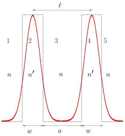
Figure 5: (Color online) Analogous optical system of the dimer structure present in our model.

This model corresponds to associate to an incident wave of energy $E=mv^{2}/2$ and wavevector $\kappa=mv/\hbar$ a transmitted wave of wavevector $\kappa^{\prime}=\kappa\sqrt{1-V_{\textmd{dis}}/E}\simeq\kappa(1-V_{\textmd{dis}}/2E)$ in the regions where the disorder potential is present. The reflection coefficient for an incident wave of wavevector $\kappa$ through the two-slab system (from region 1 to region 5, as shown in Fig. 5) can be written as

$$r_{15}=\dfrac{r_{12}+r_{25}e^{2i\alpha}}{1+r_{12}r_{25}e^{2i\alpha}}$$ (14)

with

$$\begin{split}r_{25}=&\dfrac{r_{23}+r_{35}e^{2i\beta}}{1+r_{23}r_{35}e^{2i\beta}}\\ r_{35}=&\dfrac{r_{34}+r_{45}e^{2i\alpha}}{1+r_{34}r_{45}e^{2i\alpha}}\\ \end{split}$$ (15)

where $\alpha=\frac{n}{n^{\prime}}\kappa w$, $\beta=\kappa a$, $r_{34}=r_{12}=-r_{23}=-r_{45}=(n-n^{\prime})/(n+n^{\prime})$. Equation (14) takes the form

$$\begin{split}&r_{15}=r_{12}\times\\ &\dfrac{\left[-1-2e^{2i\alpha}+e^{2i\beta}+r_{12}^{2}e^{4i\alpha}+r_{12}^{2}e^{2i(\alpha+\beta)}-2e^{2i(\beta+2\alpha)}\right]}{1-2r_{12}^{2}e^{2i\alpha}+r_{12}^{2}e^{4i\alpha}+r_{12}^{2}e^{2i\beta}-2r_{12}^{2}e^{2i(\alpha+\beta)}+2r_{12}^{4}e^{2i(2\alpha+\beta)}}\\ \end{split}$$ (16)

The behavior of the reflectivity $\mathcal{R}=|r_{15}|^{2}$ of the dimer structure must be compared with that of a single bump

$$|r_{13}|^{2}=\left|\dfrac{r_{12}(1-e^{2i\alpha})}{1-r^{2}_{12}e^{2i\alpha}}\right|^{2}.$$ (17)

This is shown in Fig. 6. For our choice of the parameters, the reflectivity of the dimer oscillates with respect to that of a single bump that decreases monotonically, in qualitative agreement with what observed for the localization fraction shown in Fig. 4. The shift of the minimum position for the dimer reflectivity with respect to the localization may be attributed to on the one hand, the Gaussian shape of bumps as compared to the rectangular shape of the dielectric slabs, and on the other hand to the inhomogeneity and non-linearity of the system. All these factors are not taken into account in the current optical model. Finally, let us remark that both the single bump and the single dimer yield full delocalization ($\mathcal{R}=0$) for $\alpha=\pi$, namely when each bump plays the role of a cavity Dunlap et al. (1990); Schaff et al. (2010), corresponding to $v\gg c$ in our system.

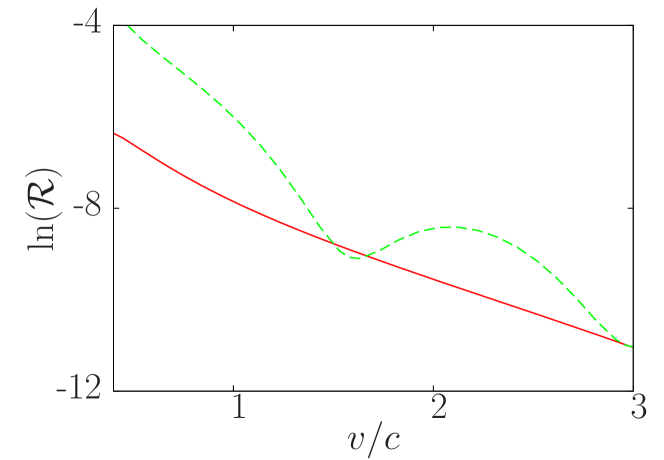
Figure 6: (Color online) Reflectivity (in logarithmic scale) of a single defect (red continuous line) and of a dimerized structure (green dashed line) as a function of the disorder potential velocity.

III.2 Random distribution of impurities

As already illustrated in Sec. II.2, we consider three sets of parameters for the AM and RDM potentials: (i) a bump density $n_{\textmd{{dis}}}\simeq 0.12\lambda^{-1}\simeq 0.16$ peaks/$\mu$m, and $d=\lambda$; (ii) a bump density $n_{\textmd{{dis}}}\simeq 0.5\lambda^{-1}\simeq 0.65$ peaks/$\mu$m, and $d=\lambda$; and (iii) with the same bump density as in (ii) but with $d=\lambda/2$. In the three cases, the size of the disorder potential is $485$ $\mu$m and the BEC size is 204 $\mu$m.

We run the simulations for up to approximately 3-4 cycles of $\omega_{z}$. We generally note that in our range of drift velocities, longer time durations are not necessary since the moving disorder potential would try to bring the condensate too high up along the harmonic potential and thus the condensate would inevitably fall back at $z_{f}$.

We run simulations for 37 different drift velocities, in the range $v=[0.46-1.30]c=[1.40-3.98]\textmd{mm/s}$ (where $c=3.06\textmd{mm/s}$), with between 3 and 24 random potential realizations for each drift velocity. To obtain the percentage of localized atoms, we compute the distance traveled by the condensate center-of-mass corresponding to a fixed value of the potential drift. We used that unique velocity-independent distance, in our case $\Delta z_{\textmd{dis}}=96\mu$m, in order to compare equivalent final potential configurations. For this value of $\Delta z_{\textmd{dis}}$, we measure a small center-of-mass displacement $\Delta z_{\mathrm{c.m.}}$, generally lower than an oscillator harmonic length in the axial direction, $\Delta z_{\mathrm{c.m.}}<a_{z}=\sqrt{\hbar/(m\omega_{z})}$. Then we identify the ratio $N_{loc}/N$ with the ratio between the center-of-mass shift and $\Delta z_{\textmd{dis}}$ according to Eq. (10). Figure 7 shows the localized ratio $N_{loc}/N$ for the potentials (i), (ii) and (iii). We first note that irrespective of the kind of disorder the localization occurs for $v>0.5c$. This unexpected localization regime may be due to the local sound velocity being inhomogeneous due to the harmonic confinement Capuzzi et al. (2011) or to the non-vanishing amplitude of the disorder potential Ianeselle et al. (2006). $N_{loc}/N$ is very small for all data sets, except for the parameters (ii) at $v\simeq 1.1c$, for both AM and RDM (see the middle plot in Fig. 7). We claim that this is an effect related to the presence of dimers both in the RDM by construction, and in the AM due to the choice $d=\lambda$ and density $n_{\mathrm{dis}}=0.5\lambda^{-1}$, as shown in the bottom panel of Fig. 2. Indeed, in the low density case (top panel of Fig. 7) where the AM has just developed few dimers with respect to the RDM, the localization enhancement in the RDM is well visible, even if the localization fraction is very small. Moreover, its oscillatory behavior as function of $v$ reminds that of the single dimer shown in Fig. 4, with minimal localization near $v/c\simeq 0.9$. Finally, in the bottom panel of Fig. 7 we show that the choice $d=\lambda/2$ suppresses the $N_{loc}/N$ peak at $v\simeq 1.1c$, since it destroys the correlations introduced by the single dimer itself (cf. Fig. 3).

In Fig. 8 we plot the turning point $z_{f}$ for the AM with $n_{\textmd{dis}}=0.5\lambda^{-1}$ and $d=\lambda/2$ and the RDM with the same peak density but with $d=\lambda$. We verified numerically that for the disorder amplitude and velocities considered the turning point $z_{f}$ is proportional to the average drag force $\bar{F}_{\textmd{dis}}$ as expected from Eq. (12) in the limit of small displacements. Not surprisingly, the overall behavior of the average drag force $\bar{F}_{\textmd{dis}}$ is qualitatively similar to the localization ratio, showing that to a greater drag force, i.e., less superfluid fraction, it corresponds a higher localization efficiency. In agreement with the single defect analysis (Sec. III.1), in both Figs. 7 and 8, we clearly observe a partial suppression of the localization at $v\simeq 0.8-0.9c$, and an enhancement of the localization at a supersonic region of the drift velocities, when correlations are dominant.

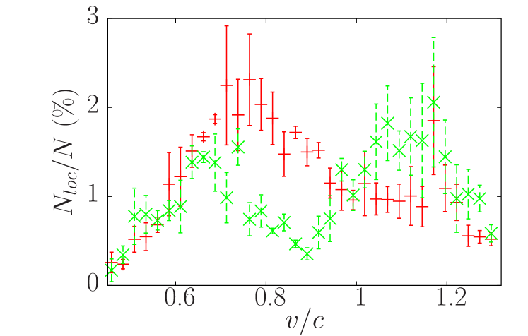
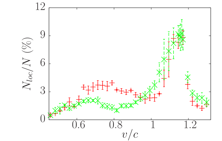
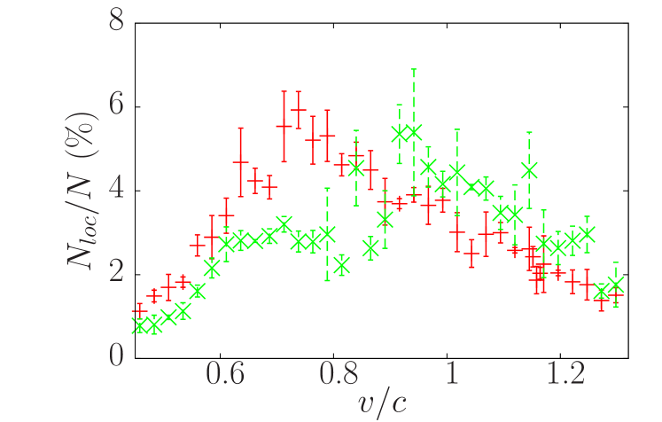
Figure 7: (Color online) Localized BEC fraction as a function of the disorder potential drift velocity $v$, in units of the sound speed $c$ evaluated at the center of the trap. The red crosses correspond to the AM and the green stars to the RDM. The top panel corresponds to $n_{\textmd{{dis}}}\simeq 0.12\lambda^{-1}$, and $d=\lambda$; the middle panel corresponds to $n_{\textmd{{dis}}}\simeq 0.5\lambda^{-1}$, and $d=\lambda$; the bottom panel corresponds to $n_{\textmd{{dis}}}\simeq 0.5\lambda^{-1}$, and $d=\lambda/2$.

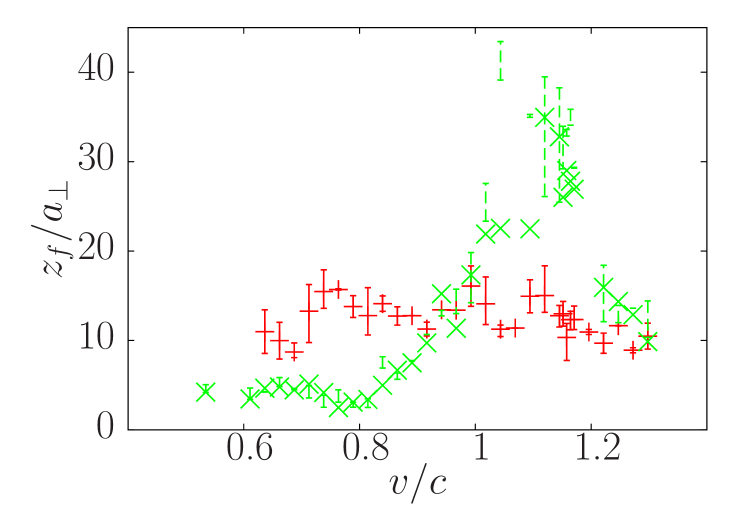
Figure 8: (Color online) Turning point $z_{f}$ as a function of the disorder potential velocity $v$, in units of the sound speed $c$ evaluated at the center of the trap. The red crosses correspond to the uncorrelated disorder with $n_{\mathrm{dis}}=0.5\lambda^{-1}$ and $d=\lambda/2$, and the green stars to the correlated one with $d=\lambda$ and the same peak density.

III.3 Localization inhomogeneity

In order to prove that we are observing the localization of a BEC fraction rather than a slower drag of the whole BEC, we analyze the dynamics of the BEC tails, where the density is lower and AL should occur more efficiently. In particular, we focus on the forward moving tail distribution that experiences the disorder potential for the whole simulation time. Analogously to Sec. III.2, we compute the percentage of atoms localized in the forward moving tail of the condensate $N_{loc,t}/N_{t}$ by dividing the tail center-of-mass shift with the same $\Delta z_{\textmd{dis}}$ value. We looked at 3 different sizes of that tail: those comprising 1%, 5% and 10% of the total condensate mass. In the case of the forward tails that amounts to 1% of the total condensate mass (see Fig. 9), we observe an almost complete localization in that same supersonic region of the drift velocities. While for the 5% and 10% mass tails (not shown), we measure   50% of localization efficiency. The negative values of localization in the subsonic region of drift velocities are due to the fluctuations of the condensate density caused by the presence of the disorder potential. At those velocities, these fluctuations provoke the forward leading small portion of mass to buckle back towards the center of the condensate even though there is no much overall motion of the whole condensate.

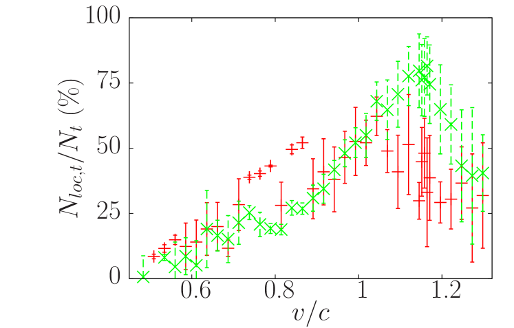
Figure 9: (Color online) Localized BEC fraction of the leading moving tail -1% of the total condensate mass- as a function of the disorder potential velocity $v$, in units of the sound speed $c$ evaluated at the center of the trap. The red crosses correspond to the AM (iii) and the green stars to the RDM (ii).

IV Conclusions

We have presented an analysis of the drag properties of two kinds of disorder potentials of finite extent moving through an inhomogeneous quasi-1D Bose-Einstein condensate. Because of the presence of the external harmonic confinement our system, unlike Paul et al. (2009), is never in a stationary state. We treated both cases of non-correlated and correlated disorder with short-range correlations. Our numerical computation of the fraction of localized atoms and the drag force shows that for the case of correlated disorder, in the form of random dimers, there is a suppression or an enhancement of localization depending on the drift velocity. This was buttressed by our analytical optical model in which we determined the reflectivity of a single dimer and of a lonely defect. The effects of correlations are masked as we increase the disorder density and the dimers cannot be distinguished from a high density collection of single defects.