Abstract

We present results about large deviations and laws of large numbers for various polymer related quantities.

In a completely general setting and strictly positive temperature, we present results about large deviations for directed polymers in random environment. We prove quenched large deviations (and compute the rate functions explicitly) for the exit point of the polymer chain and the polymer chain itself.

We also prove existence of the upper tail large deviation rate function for the logarithm of the partition function. In the case where the environment weights have certain log-gamma distributions the computations are tractable and allow us to compute the rate function explicitly.

At zero temperature, the polymer model is now called a last passage model. With a particular choice of random weights, the last passage model has an equivalent representation as a particle system called Totally Asymmetric Simple Exclusion Process (TASEP). We prove a hydrodynamic limit for the macroscopic particle density and current for TASEP with spatially inhomogeneous jump rates given by a speed function that may admit discontinuities. The limiting density profiles are described with a variational formula. This formula enables us to compute explicit density profiles even though we have no information about the invariant distributions of the process. In the case of a two-phase flux for which a suitable p.d.e. theory has been developed we also observe that the limit profiles are entropy solutions of the corresponding scalar conservation law with a discontinuous speed function.

Chapter 1 Introduction

1.1 Polymers at finite temperature and corner growth models

We begin by presenting the two main models that are discussed in this dissertation. After the two models are introduced we offer a connection between the two of them (namely one can be viewed as a limiting case of the other). The two remaining sections of the chapter can be viewed as an informal introduction to the material that follows: Some basic definitions, discussion on classical results and an idea of the kind of questions we are asking. At the end of the chapter we describe the organization of the thesis.

1.1.1 General polymer models

A directed polymer in random environment is a random walk path that interacts with a random environment. The polymer chains live in $\mathbb{Z}^{d}\times\mathbb{Z}_{+}$, where the last coordinate denotes time. The space of environments is denoted by $\Omega=\{\omega(\mathbf{u},n):\mathbf{u}\in\mathbb{Z}^{d},n\in\mathbb{Z}_{+}\}$ and is equipped with a probability measure $\mathbb{P}$, so that under $\mathbb{P}$ the random variables $\omega(\mathbf{u},n)$ are i.i.d. for all $\mathbf{u}$, $n$.

The two models under consideration are directed polymers with free endpoints and directed polymers with constrained endpoints. Here, directed means that the last coordinate is always increasing by $1$ at each time step. This allows for the polymer chain in $d+1$ dimensions to be viewed as the path of a $d$-dimensional nearest neighbor random walk.

We assume that at time $t=0$, the starting point of the polymer chain (the random walk) is anchored at $\mathbf{0}\in Z^{d}$. For each $m\in\mathbb{N}$, define the set of possible endpoints for the polymer to be $\mathcal{E}(m)$. For a fixed $(\mathbf{u},m)$ in $\mathcal{E}(m)$, the set of all polymer chains starting from $(\mathbf{0},0)=x_{0}$ and ending at $(\mathbf{u},m)=x_{m}$ is

$$\mathcal{R}(\mathbf{u},m)=\big{\{}x_{0,m}: x_{0,m}=(x_{0},x_{1},\,...\,,x_{m}),\,x_{k}-x_{k-1}=(\pm e_{i},1)$$ (1.1)

$$\text{ for some }1\leq i\leq d,\text{ for all }1\leq k\leq m,\,(\mathbf{0},0)=x_{0},\,(\mathbf{u},m)=x_{m}\big{\}},$$

where $e_{i},1\leq i\leq d$ is the standard basis of $\mathbb{R}^{d}$.

The point-to-point partition function is defined by

$$Z^{\beta}(\mathbf{u},m)=\sum_{x_{0,m}\in\mathcal{R}(\mathbf{u},m)}\prod_{j=1}^{m}e^{\beta\omega(x_{j})},$$ (1.2)

and the total (or the point-to-line) partition function can be defined by

$$Z^{\beta}_{m}=\sum_{\mathbf{u}\in\mathcal{E}(m)}\sum_{x_{0,m}\in\mathcal{R}(\mathbf{u},m)}\prod_{j=1}^{m}e^{\beta\omega(x_{j})},$$ (1.3)

The parameter $\beta$ is what is known in the literature as the inverse temperature and is assumed without loss of generality to be positive.

Under a fixed environment $\omega$, the polymer chain $x_{0,m}$ is selected according to the quenched probability measures

$$Q^{\omega,\beta}_{\mathbf{u},m}\{x_{0,m}\}=(Z^{\beta}(\mathbf{u},m))^{-1}\prod_{j=1}^{m}e^{\beta\omega(x_{j})},$$ (1.4)

and

$$Q^{\omega,\beta}_{m}\{x_{0,m}\}=(Z^{\beta}(m))^{-1}\prod_{j=1}^{m}e^{\beta\omega(x_{j})},$$ (1.5)

respectively for each of the models described above.

Let us momentarily restrict our attention to dimension $1+1$. The polymer chain starts by being anchored at $(0,0)$ and under a fixed environment, at time $n$ the chain is chosen according to the measures $Q^{\omega,\beta}$. The chain lives inside the cone $\{\mathbf{u}=(u_{1},u_{2})\in\mathbb{Z}\times\mathbb{Z}_{+}:u_{2}\geq|u_{1}|\}$. We rotate the picture clockwise by $45$ degrees. The polymer chain now becomes a path $\tilde{x}_{0,m}=\{(0,0)=x_{0},x_{1},\cdots,x_{m}\}$ in the first quadrant $\mathbb{Z}_{+}^{2}$ where the differences $x_{k}-x_{k-1}$ are a standard basis vector. Such a path we call an up-right path.

The advantage of this viewpoint resides in the point-to-point model: For any vector $\mathbf{u}\in\mathbb{Z}_{+}^{2}$ we specify as an endpoint, it is guaranteed that exponentially many paths start at $(0,0)$ and end at $\mathbf{u}$, i.e. $\mathbf{u}$ is an admissible endpoint. Unfortunately we lose information about the time (now the time axis is the main diagonal) but this does not affect the analysis and the limits of the main theorems.

From this point onwards, all models in this dissertation are about paths that live in the first quadrant and are up-right paths. We denote the set of up-right paths from $(0,0)$ to $(\mathbf{u})$ by $\Pi(\mathbf{u})$. More precise details are available in the following chapters.

1.1.2 Corner growth model

The corner growth model in two dimensions is a model of a randomly growing cluster that over time covers larger and larger portions of the first quadrant $\mathbb{Z}^{2}_{+}$. At the outset, each coordinate $(i,j)$ is given a weight $\omega(i,j)$. In the language of the previous section, we have now a fixed environment and we want to study the evolution of the random cluster according to the following rules.

The general rule is that $\omega(i,j)$ is the time it takes for the random evolution to occupy site $(i,j)$. This can only be done only after its two neighbors to the left and below are either occupied or lie outside $\mathbb{Z}^{2}_{+}$. At the boundaries the rule is that point $(0,0)$ needs no occupied neighbors to start, points $(1,j)$ on the left boundary wait only for the neighbor below to be occupied, and points $(i,1)$ on the bottom boundary wait only for the left neighbor to be occupied (see Fig. 1).

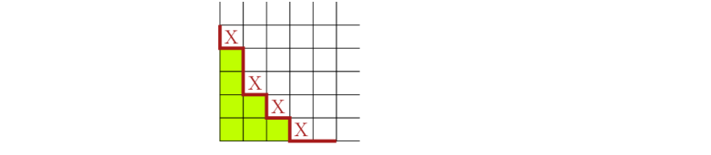
Figure 1: The shaded squares represent sites that are occupied at this particular time. The thick line represents the boundary of the cluster and the squares marked with $X$ are the “ growth sites ”. The time it takes each growth site to be infected (shaded) is $\omega_{0,4},\omega_{1,2},\omega_{2,1},\omega_{3,0}$ respectively. These times start elapsing as soon as both the left and lower neighbors become shaded.

The quantity of interest is that of the last passage time. Given a site $(i,j)$ the last passage time, $T(i,j)$, is the time when the site $(i,j)$ becomes part of the evolving cluster. Using the evolution described above, it can be recursively computed (with appropriate boundary conditions) to be

$$T(i,j)=T(i-1,j)\vee T(i,j-1)+\omega_{i,j}.$$ (1.6)

Equation (1.6) says that $(i,j)$ becomes part of the cluster only after both $(i-1,j)$ and $(i,j-1)$ are part of the cluster, and after that happens, time $\omega_{i,j}$ elapses. Assume without loss that $T(0,0)=\omega(0,0)=0$. An easy induction argument then yields that

$$T(i,j)=\max_{x_{0,i+j}\in\Pi(i,j)}\sum_{k=1}^{i+j}\omega_{x_{k}}.$$ (1.7)

In the case where the $\omega$ weights are continuous and an endpoint $\mathbf{u}=(i,j)$ is specified, there is a unique path $x_{0,i+j}$ for $\mathbb{P}$- a.e. $\omega$ that attains the last passage time. We call that the maximal path and denote it by $x^{\text{max}}_{0,i+j}$. In this respect, we can define a (degenerate) quenched measure on the paths,

$$\widetilde{Q}^{\omega}_{\mathbf{u},i+j}\{x_{0,i+j}\}=\delta_{x^{\text{max}}_{0,i+j}}=\begin{cases}1,&x_{0,i+j}=x^{\text{max}}_{0,i+j}\\ 0,&\text{otherwise.}\end{cases}$$ (1.8)

If the $\omega$ weights have discrete distributions, is possible that there are more than one maximal path. When that happens, the quenched probability measure on the paths is the uniform measure on maximal paths.

1.1.3 Connection of the two models

Now we are ready to justify the title of this dissertation. The connection between the polymer models and the last passage time models comes via the parameter $\beta$. As we let $\beta$ tend to $\infty$, under a fixed environment, the quenched probability measure $Q^{\omega,\beta}$ converges weakly to a delta mass, given by (1.8). This becomes precise in the context of the next proposition.

Proposition 1.1.

Let $\mathbf{u}\in\mathbb{Z}^{2}_{+}$, $\mathbf{u}=(i,j)$ and let $m=i+j$. Fix an environment $\omega$. Then, the probability measures defined by (1.4) converge weakly

$$Q^{\beta,\omega}_{\mathbf{u},m}\{x_{0,m}\}\Longrightarrow\widetilde{Q}^{\omega}_{\mathbf{u},m}\{x_{0,m}\}=\delta_{x^{\text{max}}_{0,i+j}},\quad\text{as }\beta\to\infty.$$ (1.9)

Proof.

Let $f$ a function on the space $\Pi(\mathbf{u})$ of up-right paths. Then

$$\int_{\Pi(\mathbf{u})}f\,dQ^{\beta,\omega}_{\mathbf{u},m} =\sum_{x_{0,m}\in\Pi(\mathbf{u})}f(x_{0,m})Q^{\beta,\omega}_{\mathbf{u},m}\{x_{0,m}\}$$

$$=\sum_{x_{0,m}\in\Pi(\mathbf{u})}f(x_{0,m})Z^{\beta}({\mathbf{u},m})^{-1}\prod_{j=1}^{m}e^{\beta\omega(x_{j})}$$

$$=f(x_{0,m}^{\text{max}})Z^{\beta}({\mathbf{u},m})^{-1}\prod_{j=1}^{m}e^{\beta\omega(x^{\max}_{j})}$$

$$\phantom{xxxxxxxxxx}+\sum_{\begin{subarray}{c}x_{0,m}\in\Pi(\mathbf{u})\\ x_{0,m}\neq x_{0,m}^{\text{max}}\end{subarray}}f(x_{0,m})Z^{\beta}({\mathbf{u},m})^{-1}\prod_{j=1}^{m}e^{\beta\omega(x_{j})}$$

$$=f(x_{0,m}^{\text{max}})Z^{\beta}({\mathbf{u},m})^{-1}\prod_{j=1}^{m}e^{\beta\omega(x^{\max}_{j})}$$ (1.10)

$$\phantom{xxxxxxxxxx}\times\Bigg{(}1+\sum_{\begin{subarray}{c}x_{0,m}\in\Pi(\mathbf{u})\\ x_{0,m}\neq x_{0,m}^{\text{max}}\end{subarray}}f(x_{0,m})e^{\sum_{j=1}^{m}\beta(\omega(x_{j})-\omega(x^{\text{max}}_{j}))}\Bigg{)}$$ (1.11)

As $\beta\to\infty$, (1.11) tends to $1$ because all the exponents are negative. We are going to show that $Z^{\beta}({\mathbf{u},m})^{-1}\prod_{j=1}^{m}e^{\beta\omega(x^{\max}_{j})}$ tend to $1$ as $\beta\to\infty$. Then the proposition follows from (1.10) and $\eqref{bbbbb}$.

From the definitions, $Z^{\beta}({\mathbf{u},m})^{-1}\prod_{j=1}^{m}e^{\beta\omega(x^{\max}_{j})}\leq 1$. For a lower bound, observe that for any $\delta>0$ and $\beta$ sufficiently large

$$Z^{\beta}({\mathbf{u},m})\Big{(}\prod_{j=1}^{m}e^{\beta\omega(x^{\max}_{j})}\Big{)}^{-1} =\sum_{x_{0,m}\in\Pi(\mathbf{u})}e^{\sum_{j=1}^{m}{\beta(\omega(x_{j})-\omega(x^{\max}_{j}))}}$$

$$=1+\sum_{\begin{subarray}{c}x_{0,m}\in\Pi(\mathbf{u})\\ x_{0,m}\neq x_{0,m}^{\text{max}}\end{subarray}}e^{\sum_{j=1}^{m}{\beta(\omega(x_{j})-\omega(x^{\max}_{j}))}}$$

$$\leq 1+\delta.\quad\quad\quad\phantom{xxxxxxxxxxxxxxxxxxxx}\qed$$

1.2 Large deviations

The theory of large deviations is concerned with the study of rare (improbable) events. Assume you have a sequence $\{X_{n}\}_{n\in\mathbb{N}}$ of real random variables on $\Omega$. A natural question that arises is to compute the limiting probability $\lim_{n\to\infty}\mathbb{P}\{X_{n}\in A\}$ where $A$ is a fixed measurable set on $\mathbb{R}$. When the events $\mathcal{A}_{n}=\{X_{n}\in A\}$ are “rare” the limiting probability can be $0$. This information, while not particularly helpful, leads to a deeper question: How fast does it go to $0$? For example if the probabilities are now summable, one can apply the Borel-Cantelli lemma.

In a more general setting, instead of a sequence of random variables, one can use a sequence of probability measures $\mu_{n}$ on a Polish measurable space $\mathcal{X}$ (in the example above, $\mu_{n}=\mathbb{P}\{X_{n}\in\cdot\}$ and $\mathcal{X}=\mathbb{R}$). The measures $\mu_{n}$ live in the space of probability measures on $\mathcal{X}$, $\mathcal{M}_{1}(\mathcal{X})$ and we say that they satisfy a large deviation principle if the following definition holds.

Definition 1.2.

Let $I:\mathcal{X}\mapsto[0,\infty]$ be a lower semicontinuous function and $r_{n}\to\infty$ a sequence of positive constants. A sequence of probability measures $\{\mu_{n}\}_{n}\subseteq\mathcal{M}_{1}(\mathcal{X})$ is said to satisfy a large deviation principle with rate function $I$ and normalization $r_{n}$ if the following inequalities hold for all closed $F\subseteq\mathcal{X}$ and all open $G\subseteq\mathcal{X}$:

$$\varlimsup_{n\to\infty}\frac{1}{r_{n}}\log\mu_{n}(F)\leq-\inf_{F}I;$$ (1.12)

$$\varliminf_{n\to\infty}\frac{1}{r_{n}}\log\mu_{n}(G)\geq-\inf_{G}I;$$ (1.13)

When the sets $\{I\leq c\}$ are compact for all $c\in\mathbb{R}$, we say $I$ is a tight rate function. It is of interest to find explicit rate functions, since they offer an exact measurement of the rare event. For example, insurance companies can use that information to decide on a fair premium for the customer.

1.3 Interacting particle systems and hydrodynamic limits

In full generality, interacting particle systems consist of finitely or infinitely many particles that evolve in space and time according to given transition probabilities or rates, with some interaction rules imposed on the particles. A particle system that has been extensively studied, is the Totally Asymmetric Simple Exclusion Process (TASEP). It is intimately connected with the last passage time, assuming exponential weights.

Assume that particles occupy integer sites. There is at most one particle at each site (Simple). Each particle attempts to move one unit to the right (Totally Asymmetric) with rate $1$ . The jump is suppressed with probability $1$ if the target site is occupied (Exclusion).

One-dimensional TASEP can be constructed graphically by assigning independent mean $1$ Poisson processes (called clocks) on each integer site. The vertical direction now becomes time. As time progresses, a particle on site $i$ attempts to jump at the Poisson event times of the site it occupies, and the jump happens with probability $1$ as long as the exclusion rule is satisfied. With probability 1, two adjacent Poisson processes cannot have simultaneous events, and for every time $t$ there are infinitely many Poisson processes with no events before $t$, so one can study the temporal evolution of the system up to time $t$ in a rectangle $[-M,N]\times[0,t]$ around the origin.

The coupling with the corner growth model follows if we run a TASEP starting from step initial conditions: particles start by occupying only the negative integers and are labeled so that particle $i$ starts on site $-i$. Then the last passage time $T(m,n)$ is equal in distribution to the time it takes the $n$-th particle to reach site $m-n$.

Consider a sequence of exclusion processes $\eta^{n}=(\eta^{n}_{i}(t):i\in\mathbb{Z},\,t\in\mathbb{R}_{+})$ indexed by $n\in\mathbb{N}$. For each $i$ and fixed $t$, $\eta^{n}_{i}(t)=1$ if and only if there is a particle present at site $i$, at time $t$. These processes are constructed on a common probability space that supports the initial configurations $\{\eta^{n}(0)\}$ and the Poisson clocks of each process. The clocks of process $\eta^{n}$ are assumed to be independent of its initial state $\eta^{n}(0)$.

Starting from arbitrary particle initial conditions and for fixed time $t$ define the sequence of occupation measures

$$\mu^{n}_{t}([a,b])=\frac{1}{n}\sum_{i=\lfloor{na}\rfloor+1}^{\lfloor{nb}\rfloor}\eta^{n}_{i}(nt)=\frac{1}{n}\sharp\{\text{ particles in }[na,nb]\text{ at time }nt\}.$$ (1.14)

Under some regularity assumptions on the initial conditions, it is known (e.g. [27]) that this sequence of measures converges weakly for all $t$

$$\lim_{n\rightarrow\infty}\mu^{n}_{t}([a,b])=\int_{a}^{b}\rho(x,t)\,dx,$$ (1.15)

where $\rho(x,t)$ (called the particle density function) is the unique entropy solution to the scalar conservation law

$$\partial_{t}(\rho(x,t))+\partial_{x}F(x,\rho(x,t))=0.$$ (1.16)

The initial conditions of the particles correspond to the initial conditions required for uniqueness of the weak solution in (4.19) and $F$ is the particle flux of TASEP, given by $F(x,\rho)=\rho(1-\rho)$. Results of this type go by the name of hydrodynamic limit and there are many known generalizations.

1.4 Motivation

Upper tail large deviations for the last passage time have been computed in the case of geometric and exponential weights (see [17, 26]). In [26], the rate function was computed via the height function and information about equilibrium distributions for TASEP particles. The equilibrium distributions for TASEP is a result of Burke’s theorem for M/M/1 queues and they can be interpreted as appropriate boundary weights in the corner growth model. This (Burke) property is “transferable” to the log-gamma polymer model. The model was introduced in [29]. The model is a $1+1$ dimensional polymer model at temperature $\beta=1$ where for a fixed $\mu>0$, the weights

$$\omega(i,j)=-\log Y_{i,j},\quad\text{ and }Y_{i,j}\sim\text{Gamma}(\mu)$$

for $(i,j)\in\mathbb{N}^{2}$.

1.5 Organization

We start (Chapter 2) by describing general polymer models. In Chapter 2 we show some general facts about the partition function and proceed by showing quenched large deviation results for the polymer chains under the quenched measures (1.4), (1.5). In a completely general setting we show some quantitative properties of the rate functions (existence, continuity, large $\beta$ behavior).

In Chapter 3 we restrict to a specific $1+1$ dimensional model, the log-gamma model that satisfies a certain property that allows for explicit computations. We present large deviation results about the logarithm of the partition functions.

The following two chapters (Chapters 4 and 5) are concerned about hydrodynamic limits of exclusion processes and last passage time where the weights $\omega$ are now exponential but with different parameters (so they are not identically distributed). The parameters are decided using a (possibly discontinuous) function $c(x)$. The connection with the particle process TASEP leads to a further connection with scalar conservation laws with discontinuous coefficients.

Chapter 2 Generalities about Polymer Models

2.1 Introduction

2.1.1 Directed polymers with constrained endpoint in a rectangle

For $\mathbf{u}\in\mathbb{Z}^{d}_{+}$ define the set of directed polymer chains from $\mathbf{v}$ to $\mathbf{u}$ with $\|\mathbf{u}-\mathbf{v}\|_{1}=m$

$$\Pi_{\mathbf{v}}(\mathbf{u}) =\big{\{}x_{\centerdot}=\{\mathbf{v}=x_{0},x_{1},\dotsc,x_{m}=\mathbf{u}\}:x_{k}\in\mathbb{Z}^{d}_{+},$$

$$\phantom{zxxxxxxxxxxxxxbbbbbbxxxxxxxxxx}x_{k+1}-x_{k}=\mathbf{e}_{i}\text{ for some }1\leq i\leq d\big{\}},$$ (2.1)

where $e_{i}$ is the $i$-th standard basis vector.

The point-to-point partition function is in this case defined by

$$Z^{\beta}_{\mathbf{v},\mathbf{u}}=\sum_{x_{\centerdot}\in\Pi_{\mathbf{v}}(\mathbf{u})}\prod_{j=1}^{m}e^{\beta\omega(x_{j})}=\sum_{x_{\centerdot}\in\Pi_{\mathbf{v}}(\mathbf{u})}e^{\beta\sum_{j=1}^{m}\omega(x_{j})}.$$ (2.2)

In the special case where $\mathbf{v}=\mathbf{0}$ we omit the index $\mathbf{v}$ from the above notation: The partition function is denoted by $Z^{\beta}_{\mathbf{u}}$ and the set of polymer chains by $\Pi(\mathbf{u})$. Observe that in the definitions given so far, the weight at the starting point is ignored. When that is not the case, we denote

$$Z^{\beta,\square}_{\mathbf{v},\mathbf{u}}=e^{\beta\omega(\mathbf{v})}Z^{\beta}_{\mathbf{v},\mathbf{u}}.$$

Under a fixed environment $\omega$, fixed endpoint $\mathbf{u}$ and fixed inverse temperature $\beta$, the quenched probability measure $Q^{\omega,\beta}_{\mathbf{u}}$ on paths with constrained endpoints, is defined by

$$Q^{\omega,\beta}_{\mathbf{u}}(x_{\centerdot})=\big{(}Z^{\beta}_{\mathbf{u}}\big{)}^{-1}\prod_{j=1}^{m}e^{\beta\omega(x_{j})}.$$ (2.3)

2.1.2 Directed polymers with constrained endpoint in a rectangle

In this variation we fix the number of time steps $m$. Define the set of all admissible polymer chains starting from $\mathbf{0}$ to be

$$\Pi_{\operatorname{tot}}(m) =\big{\{}x_{0,m}:x_{0,m}=\big{\{}x_{0},x_{1},\ ,...\,x_{m}\big{\}},\,x_{k+1}-x_{k}=e_{i}$$ (2.4)

$$\phantom{xxxxxxxxxxxxxxxxxxxxxxxxxxx}\text{ for some }1\leq i\leq d,\text{ for all }1\leq k\leq m\big{\}}$$

where $e_{i},1\leq i\leq d$ is the standard basis of $\mathbb{R}^{d}$.

For each $m>0$, the total partition function is defined by

$$Z^{\beta,\operatorname{tot}}_{m}=\sum_{\mathbf{u}\in\mathbb{Z}_{+}^{d}:\|\mathbf{u}\|_{1}=m}Z^{\beta}_{\mathbf{u}}.$$ (2.5)

The corresponding quenched probability measure $Q^{\omega,\beta}_{m}$ on paths in $\Pi_{\operatorname{tot}}(m)$, is

$$Q^{\omega,\beta}_{m}(x_{0,m})=\big{(}Z^{\beta,\operatorname{tot}}_{m}\big{)}^{-1}\prod_{j=1}^{m}e^{\beta\omega(x_{j})}.$$ (2.6)

Remark 2.1.

If the rectangle has dimension $2$, then both models describe the classical directed random polymers in random environment in dimension 1+1 described in the introduction (point-to-point and free endpoint respectively), where the picture is rotated by 45 degrees, so the polymer lives in the first quadrant.

2.1.3 Known results

Concentration inequalities.

A problem in the area of random polymers in random environment is about the fluctuations (in particular the fluctuation exponent) of $\log Z^{\beta}_{m}$ that is conjectured to be $2/3$ in the physics literature. Rigorous results about upper and lower bounds for fluctuations exponents for specific polymer models can be found in [8, 12, 20, 22, 33, 34]. The only two cases where the conjectured value of $2/3$ is in fact verified is the log-gamma polymer [29] and the brownian polymer [30].

In absence of exact variance bounds, information can be derived from concentration inequalities. In [9] an exponential of order $n^{1/3}$ concentration result has been obtained for the partition function in a Gaussian environment and later this had been generalized for all weights under certain exponential moment assumptions in [11].

The sharpest concentration inequalities are exponential of order $n$, proven in [19, 32] and a certain version used here about the point-to-point free energy in [13].

Large deviations.

The exponential order $n$ concentration inequality for the partition function is the correct one for the upper tail large deviations and is the correct normalization in order to get a non-trivial upper tail rate function.

For the lower tail the behavior depends on the distribution of the weights. In [7] three different normalization regimes for the lower tails are shown, depending on the distribution of the weights. It is also mentioned that a normalization $n^{2}$ is true if the weights are bounded. This is proved in the case where the weights are Gaussian or bounded in [9] where upper and lower normalizations are proven.

In the last part of the chapter we prove quenched large deviations for the exit point of the polymer (in the free endpoint case) and quenched large deviations for the polymer path in both the free endpoint and constrained endpoint. The results are described in further detail in Section 4.2.

Notation and conventions.

Throughout we use $\mathbb{N}$ for positive integers, while $\mathbb{Z}_{+}$ denotes the set of non-negative integer. Similarly, $\mathbb{R}_{+}$ denotes the set of non-negative real numbers and $\mathbb{R}^{d}_{+}$ is the set of all vectors with non-negative coordinates. All vectors $(v_{1},v_{2},\dotsc,v_{d})\in\mathbb{R}^{d}$ are denoted by boldface notation $\mathbf{v}=(v_{1},v_{2},\dotsc,v_{d})$. The ordering $\mathbf{v}<\mathbf{u}$ means $v_{1}\leq u_{1},v_{2}\leq u_{2},\dotsc,v_{d}\leq u_{d}$. The $d$-dimensional vector with entries equal to $1$ is denoted by $\mathbf{1}=(1,1,\dotsc,1)$ and correspondingly, $\mathbf{0}=(0,0,\dotsc,0)$. For the purposes of this dissertation we define for $\mathbf{y}=(y_{1},y_{2},\dotsc,y_{d})\in\mathbb{R}^{d}$, $n\in\mathbb{N}$ the floor of a vector $\lfloor{n\mathbf{y}}\rfloor=(\lfloor{ny_{1}}\rfloor,\lfloor{ny_{2}}\rfloor,\dotsc,\lfloor{ny_{d}}\rfloor)$.

2.2 Definitions and Statement of Results

Some technicalities before stating the general results. We need a technical assumption on the environment $\omega$. Henceforth we assume

Assumption 2.2.

There exists some $\xi>0$ that depends on the distributions of the weights $\omega$ such that

$$\mathbb{E}\big{(}e^{\xi|\omega(\mathbf{u})|}\big{)}<\infty.$$ (2.7)

This guarantees the existence of a large deviation rate function defined by

$$I(r)=-\lim_{\varepsilon\rightarrow 0}\lim_{n\rightarrow\infty}n^{-1}\log\mathbb{P}\Big{\{}n^{-1}\sum_{i=1}^{n}\omega(\mathbf{u}_{i})\in(r-\varepsilon,r+\varepsilon)\Big{\}}.$$ (2.8)

All results that follow are valid for $\beta<\xi$. In order to make the proofs cleaner we also assume that for all $\mathbf{u}\in\mathbb{Z}^{d}_{+}$,

$$\mathbb{P}\{\omega(\mathbf{u})\geq 0\}>0.$$ (2.9)

We start by proving some qualitative properties for the limits of the rectangle partition functions and we summarize them in the following two propositions. The superscript $\beta$ is considered fixed and henceforth omitted until the end of the chapter where it becomes relevant to take limits as $\beta\to\infty$.

Proposition 2.3.

Let $\mathbf{y}=(y_{1},y_{2},\dotsc,y_{d})\in\mathbb{R}_{+}^{d}$, $n\in\mathbb{N}$ and let $Z_{\lfloor{n\mathbf{y}}\rfloor}$ be defined by (2.2). Then the limit

$$\lim_{n\to\infty}n^{-1}\log Z_{\lfloor{n\mathbf{y}}\rfloor}=p(\mathbf{y})\quad\mathbb{P}-a.s.$$ (2.10)

Furthermore, there exists an event $\Omega_{0}\subseteq\Omega$ of full probability such that the a.s. convergence happens simultaneously for all $\mathbf{y}\in\mathbb{R}_{+}^{d}$. The limiting value viewed as a function of $\mathbf{y}$ satisfies the following properties:

1. $p(\cdot)$ is concave and continuous on $\mathbb{R}_{+}^{d}$.

2. $p(c\mathbf{y})=cp(\mathbf{y})$ for $c>0$.

3. For all $\mathbf{y}$ such that $\|\mathbf{y}\|_{1}=1$, $p(\mathbf{y})\leq p(d^{-1}\mathbf{1})$.

Proposition 2.4.

Let $n\in\mathbb{N},t>0$ and let $Z^{\operatorname{tot}}_{\lfloor{nt}\rfloor}$ be defined by (2.5). Then the limit

$$\lim_{n\to\infty}n^{-1}\log Z^{\operatorname{tot}}_{\lfloor{nt}\rfloor}=\rho^{\operatorname{tot}}(t)\quad\mathbb{P}-a.s.$$ (2.11)

Furthermore,

$$\rho^{\operatorname{tot}}(t)=\sup_{\mathbf{y}:\|\mathbf{y}\|_{1}=t}p(\mathbf{y})=p(d^{-1}t\mathbf{1})$$ (2.12)

These propositions suffice to guarantee the following general existence theorems. Then, some quantitative properties of the rate functions follow.

Theorem 2.5.

Under assumption 2.7, the following large deviations principles hold.

1. For $t>0$, $\mathbf{u}\in\mathbb{R}_{+}^{d}\setminus\{\mathbf{0}\}$ and $r\in\mathbb{R}$ there exists a nonnegative function $J$ that satisfies

   $$J_{\mathbf{u}}(r)=-\lim_{n\rightarrow\infty}n^{-1}\log\mathbb{P}\{\log Z_{\lfloor{n\mathbf{u}}\rfloor}\geq nr\}.$$ (2.13)

   $J$ is convex in the variable $(\mathbf{u},r)$ and equals 0 on the set $r\leq p(\mathbf{u})$. The rate function is continuous in $(\mathbf{u},r)$ on the set $\operatorname{int}\{(\mathbf{u},r):\mathbf{u}\in\mathbb{R}^{d}_{+}\setminus\{\mathbf{0}\},r\in\mathbb{R},J_{\mathbf{u}}(r)<\infty\}\subseteq\mathbb{R}^{d}_{+}\times\mathbb{R}$.

2. For $t>0$ and $r\in\mathbb{R}$, there exists a nonnegative function $J$ that satisfies

   $$J_{t}(r)=-\lim_{n\rightarrow\infty}n^{-1}\log\mathbb{P}\{\log Z^{\operatorname{tot}}_{\lfloor{nt}\rfloor}\geq nr\}.$$ (2.14)

   $J$ is convex in the variable $(t,r)$ and equals 0 on the set $r\leq\rho^{\operatorname{tot}}(t)$. The rate function is continuous in $(t,r)$ on the set $\operatorname{int}\{(t,r):J_{t}(r)<\infty\}$.

Next, we show some quantitative properties of the rate functions described in the following three propositions.

The first one is about the behavior of the rate function $J_{\mathbf{u}}(r)$ at the lower dimensional boundaries of $\mathbb{R}^{d}_{+}$. For a vector $\mathbf{u}=(u_{1},\ldots,u_{d})\in\mathbb{R}^{d}_{+}$ we denote by $\mathbf{u}_{1,k}=(u_{1},\ldots,u_{k},0,\ldots,0)$ the projection onto the k-dimensional facet of the first quadrant.

It is possible that $\mathbf{u}=\mathbf{0}$ so we need a definition for the rate function at $\mathbf{0}$. If we just change $\mathbf{u}$ with $\mathbf{0}$ in (2.13) the rate function becomes trivial (takes values $0$ and $\infty$ only). However, $\mathbf{0}$, is the macroscopic endpoint of the partition function. The definition of $J_{\mathbf{0}}$ should cover for example the rate function of a single random variable. It is consistent (in the sense that $\lim_{\mathbf{u}\to\mathbf{0}}J_{\mathbf{u}}(r)=J_{\mathbf{0}}(r)$ described in the following proposition) to define it the following way:

$$J_{\mathbf{0}}(r)=\begin{cases}0,&r<0,\\ x_{\infty}r,&r\geq 0\end{cases}$$ (2.15)

where $x_{\infty}\in(0,\infty]$ is the maximal slope of the one-sided Cramér rate function on the right of the zero for sums of i.i.d.  $\omega$ weights and is given by $x_{\infty}=\lim_{r\to\infty}r^{-1}I(r)$.

Proposition 2.6 (Continuity at the boundaries).

Let $\mathbf{u}\in\mathbb{R}^{d}_{+}$ and fix $r\in\mathbb{R}$. Assume that $J_{\|\mathbf{u}\|_{1}\mathbf{e}_{1}}(r)<\infty$ in a neighborhood of $\|\mathbf{u}\|_{1}\mathbf{e}_{1}$. (This is the one sided Cramér rate function.) Then, for any $k\geq 1$ and sequence $\{\mathbf{u}^{(m)}\}_{m\in\mathbb{N}}$ where $\mathbf{u}^{(m)}\leq\mathbf{u}$, $\lim_{m\to\infty}\mathbf{u}^{(m)}=\mathbf{u}_{1,k}$,

$$\lim_{m\to\infty}J_{\mathbf{u}^{(m)}}(r)=J_{\mathbf{u}_{1,k}}(r).$$ (2.16)

In the special case where $J_{\mathbf{0}}(r)<\infty$, the function $J_{(\cdot)}(r)$ is continuous everywhere on $\mathbb{R}^{d}_{+}$.

Proposition 2.7 (Unique zero).

ghoststeps

1. The rate function $J_{1}(r)$ given by (2.14) is strictly positive for $r>\rho^{\operatorname{tot}}(1)$.

2. The rate function $J_{\mathbf{u}}(r)$ given by (2.13) is strictly positive for $r>p(\mathbf{u})$.

As stated in the introduction, the polymer model starts behaving like the last passage time model when $\beta\to\infty$. For a fixed $\mathbf{u}$, define the last passage time as in (1.7). Assumption 2.7 along with the subadditive ergodic theorem, give the existence of a finite limiting last passage time constant

$$\lim_{n\to\infty}n^{-1}T(\lfloor{n\mathbf{u}}\rfloor)=\psi(\mathbf{u}),$$

with arguments identical to those used in the proof of Proposition 2.3. In turn, one can show the existence of an upper tail large deviation rate function for the last passage time, following the steps of the proof of Theorem 2.5. The rate function is given by

$$I^{\infty}_{\mathbf{u}}(r)=-\lim_{n\to\infty}n^{-1}\log\mathbb{P}\{T(\lfloor{n\mathbf{u}}\rfloor)\geq nr\}.$$

The rate functions also start behaving similarly as described in the following proposition.

Proposition 2.8 (Large $\beta$ behavior).

Let $\mathbf{u}\in\mathbb{R}^{d}_{+}$ and assume $I^{\infty}_{\mathbf{u}}(r)$ is left continuous at $r\in\mathbb{R}$. Then

$$\lim_{\beta\to\infty}J^{\beta}_{\mathbf{u}}(\beta r)=I^{\infty}_{\mathbf{u}}(r).$$ (2.17)

We also prove quenched large deviations for the exit point for the free endpoint models, and the path of a polymer chain for both models.

Theorem 2.9 (Exit point LDP).

Let $\mathbf{u}=(u_{1},u_{2},\dotsc,u_{d})\in\mathbb{R}^{d}_{+}$ with $\|\mathbf{u}\|_{1}=1$ and let $\mathbf{y}=(u_{1},\dotsc,u_{d-1})\in\mathbb{R}^{d-1}_{+}$. For $n\in\mathbb{N}$ let $[n\mathbf{u}]=(\lfloor{n\mathbf{y}}\rfloor,n-\|\lfloor{n\mathbf{y}}\rfloor\|_{1})$ and denote by $x_{n}$ the last point of the polymer chain $x_{0,n}$. Then

$$p(d^{-1}\mathbf{1})-p(\mathbf{u})=-\lim_{n\rightarrow\infty}n^{-1}\log Q^{\omega}_{n}\{x_{n}=[n\mathbf{u}]\}.$$ (2.18)

This readily leads to the following path large deviations.

Theorem 2.10 (Path LDP).

Let $\gamma:[0,1]\to\mathbb{R}_{+}^{d}$ be a coordinatewise nondecreasing Lipschitz curve with $\gamma(0)=0$. For $\varepsilon>0$ let $\mathcal{N}_{\varepsilon}(\gamma)$ denote a uniform $\varepsilon$-neighborhood of $\gamma$. The following large deviation principles hold:

1. (Constrained endpoint.) Let $\mathbf{u}$ in $\mathbb{R}_{+}^{d}$ and let $\gamma(1)=\mathbf{u}$. Then,

   $$p({\mathbf{u}})-\int_{0}^{1}p({\gamma^{\prime}(t)})\,dt=-\lim_{\varepsilon\to 0}\lim_{n\rightarrow\infty}n^{-1}\log Q^{\omega}_{\lfloor{n\mathbf{u}}\rfloor}\big{\{}x_{\centerdot}\in n\mathcal{N}_{\varepsilon}(\gamma)\big{\}}$$ (2.19)

2. (Free endpoint.) Let $\|\gamma(1)\|_{1}=1$ . Then,

   $$p(d^{-1}{\mathbf{1}})-\int_{0}^{1}p(\gamma^{\prime}(t))\,dt=-\lim_{\varepsilon\to 0}\lim_{n\rightarrow\infty}n^{-1}\log Q_{n}^{\omega}\big{\{}x_{0,n}\in n\mathcal{N}_{\varepsilon}(\gamma)\big{\}}$$ (2.20)

Remark 2.11.

The theorem is true for any curve $\gamma$ that admits a Lipschitz parametrization. It is easy to check that the rate functions in (2.10) are independent of any $C^{1}$ parametrization $\phi:[0,1]\to[0,1]$. It follows from the $1$- homogeneity of $p$ and a change of variables in the integral.

2.3 Preliminaries

In this section we record results that are used throughout. In particular, basic properties of the partition functions; their laws of large numbers and the proof of Propositions 2.3, 2.12. For the continuity of the partition functions at the boundary and for the unique zeros of the rate functions, we need a concentration inequality which we state first. At the end of the section we prove an auxiliary lemma about upper-tail large deviations of a sum of independent random variables and conclude the section with a basic fact that we use at various instances without alerting the reader.

Lemma 2.12 (Proposition 3.2.1 [13]).

Under assumption 2.7, there exist constants $c_{1},c_{2}\in(0,\infty)$ such that for all $\varepsilon>0$ sufficiently small

$$\mathbb{P}\{|\log Z_{n}-\mathbb{E}\log Z_{n}|>n\varepsilon\}\leq 2\exp\{-c_{1}\varepsilon^{2}n\}$$ (2.21)

and

$$\mathbb{P}\{|\log Z_{\lfloor{n\mathbf{u}}\rfloor}-\mathbb{E}\log Z_{\lfloor{n\mathbf{u}}\rfloor}|>n\varepsilon\}\leq 2\exp\{-c_{2}(\mathbf{u})\varepsilon^{2}n\}$$ (2.22)

Proof.

The proof is identical with the one in [13], p.26, tailored to these particular rectangle models. ∎

For $\mathbf{y}\in\mathbb{Z}_{+}^{d}$, define the coordinate shift operator $T_{\mathbf{y}}$ so that

$$Z_{\mathbf{u},\mathbf{v}}\circ T_{\mathbf{y}}=Z_{\mathbf{u}+\mathbf{y},\mathbf{v}+\mathbf{y}}$$ (2.23)

and observe that the random variables $\log Z_{\mathbf{u},\mathbf{v}}$ are superadditive, satisfying

$$\log Z_{\mathbf{u}+\mathbf{v}} \geq\log Z_{\mathbf{u}}+\log Z_{\mathbf{u},\mathbf{u}+\mathbf{v}}$$ (2.24)

$$=\log Z_{\mathbf{u}}+\log Z_{\mathbf{v}}\circ T_{\mathbf{u}}.$$

Proof of Proposition 2.3.

Assume without loss of generality that $\mathbb{E}(\omega(\mathbf{0}))>0$. This builds the monotonicity of the limiting free energy that will simplify the proof and makes the limiting free energy a positive function. The proof for concavity and homogeneity when $\mathbf{y}\in\mathbb{N}^{d}$ and $c\in\mathbb{N}$ follows from the subbadditive ergodic theorem. For the monotonicity of the limit, let $\mathbf{u}\leq\mathbf{v}\in\mathbb{Z}_{+}^{2}$ and for given $n$ fix a path $\pi_{n}$ from $n\mathbf{u}$ to $n\mathbf{v}$. Superadditivity gives

$$\log Z_{n\mathbf{v}}\geq\log Z_{n\mathbf{u}}+\beta\sum_{x_{j}\in\pi_{n}}\omega(x_{j}).$$ (2.25)

Taking a limit along a suitable subsequence after dividing by $n$ gives that $p(\mathbf{v})\geq p(\mathbf{u})+\|\mathbf{v}-\mathbf{u}\|_{1}\mathbb{E}(\omega(\mathbf{0}))$, hence $p$ is monotone on integer vectors.

For rational $\mathbf{y}\in\mathbb{Q}^{d}$, find a positive integer $k$ so that $k\mathbf{y}\in\mathbb{N}^{d}$ and define

$$p(\mathbf{y})=k^{-1}p(k\mathbf{y}).$$ (2.26)

Observe that homogeneity for integer $k$ gives that the value in (2.26) is independent of the choice of $k$. Homogeneity and concavity extend now to rational $c>0$ and rational $\mathbf{y}$ as follows.

Let $n\in\mathbb{N}$ and write it as $n=Mk+r$ with $r\in\{0,1,\dotsc,k-1\}$. Then

$$Mk\mathbf{y}\leq\lfloor{Mk\mathbf{y}+r\mathbf{y}}\rfloor=\lfloor{n\mathbf{y}}\rfloor\leq(M+1)k\mathbf{y}.$$ (2.27)

Hence, by the superadditivity

$$Z_{(M+1)k\mathbf{y}}\Big{(}Z_{\lfloor{n\mathbf{y}}\rfloor,(M+1)k\mathbf{y}}\Big{)}^{-1}\geq Z_{\lfloor{n\mathbf{y}}\rfloor}\geq Z_{Mk\mathbf{y}}\,Z_{Mk\mathbf{y},\lfloor{n\mathbf{y}}\rfloor}.$$ (2.28)

We show the upper bound. The lower one follows in the same manner. Observe that $\|(M+1)k\mathbf{y}-n\mathbf{y}\|_{1}\leq k\|\mathbf{y}\|_{1}$, so as $n\to\infty$, $n^{-1}\log Z_{\lfloor{n\mathbf{y}}\rfloor,(M+1)k\mathbf{y}}\to 0$ almost surely. This, along with (2.28), gives

$$p(\mathbf{y})=\lim_{n\rightarrow\infty}\frac{n-r+k}{n(n-r+k)}\log Z_{(n-r+k)\mathbf{y}}\geq\varlimsup_{n\rightarrow\infty}\frac{1}{n}\log Z_{\lfloor{n\mathbf{y}}\rfloor}.$$ (2.29)

Monotonicity follows as in the case with integer coordinates.

To extend to all vectors $\mathbf{y}$ in $\mathbb{R}^{d}_{+}$, define

$$p(\mathbf{y})=\sup\big{\{}p(\mathbf{x}_{m}):\mathbf{y}\geq\mathbf{x}_{m}\in\mathbb{Q}^{d}\big{\}}$$ (2.30)

With this definition, homogeneity follows immediately for rational $c$. For any $c>0$ pick $c_{1}$,$c_{2}$ $\in\mathbb{Q}$, so that $c_{1}<c<c_{2}$. Then

$$c_{1}p(\mathbf{y})=p(c_{1}\mathbf{y})\leq p(c\mathbf{y})\leq p(c_{2}\mathbf{y})=c_{2}p(\mathbf{y}).$$ (2.31)

Then consider sequences $c_{1}^{m}\nearrow c$ and $c_{2}^{m}\searrow c$ to get homogeneity for all $c\in\mathbb{R}_{+}$.

Superadditivity follows directly from (2.30) and concavity follows from homogeneity and superadditivity. This in turn implies continuity of $p(\cdot)$ in the interior of $\mathbb{R}^{d}_{+}$.

Finally, for the most general form of the limit for $\mathbf{y}\in\mathbb{R}^{d}_{+}$, pick rational vectors $\mathbf{u}_{1}<\mathbf{y}<\mathbf{u}_{2}$ so that for a given $\varepsilon>0$, $\|\mathbf{u}_{i}-\mathbf{y}\|_{1}<\varepsilon$. By superadditivity,

$$\log Z_{\lfloor{n\mathbf{u}_{1}}\rfloor}+\log Z_{\lfloor{n\mathbf{u}_{1}}\rfloor,\lfloor{n\mathbf{y}}\rfloor}\leq\log Z_{\lfloor{n\mathbf{y}}\rfloor}\leq\log Z_{\lfloor{n\mathbf{u}_{2}}\rfloor}-\log Z_{\lfloor{n\mathbf{y}}\rfloor,\lfloor{n\mathbf{u}_{2}}\rfloor}.$$ (2.32)

We first bound $\log Z_{\lfloor{n\mathbf{y}}\rfloor,\lfloor{n\mathbf{u}_{2}}\rfloor}$ from below using a path $\pi_{n}$ with segments on the boundary of the rectangle, parallel to the axes (following the ordering of the axes). As $n$ becomes large, the weights on $\pi_{n}$ will satisfy a strong law of large numbers,

$$\varliminf_{n\to\infty}n^{-1}\log Z_{\lfloor{n\mathbf{y}}\rfloor,\lfloor{n\mathbf{u}_{2}}\rfloor}\geq\lim_{n\to\infty}n^{-1}\sum_{j=1}^{\lfloor{n\|\mathbf{u}_{2}-\mathbf{y}\|_{1}}\rfloor}\beta\omega(\mathbf{x}_{j})\geq 0.$$ (2.33)

Symmetric bounds hold for $Z_{\lfloor{n\mathbf{u}_{1}}\rfloor,\lfloor{n\mathbf{y}}\rfloor}$. These, along with (2.32) give

$$p(\mathbf{u}_{1})\leq\varliminf_{n\rightarrow\infty}n^{-1}\log Z_{\lfloor{n\mathbf{y}}\rfloor}\leq\varlimsup_{n\to\infty}n^{-1}\log Z_{\lfloor{n\mathbf{y}}\rfloor}\leq p(\mathbf{u}_{2}).$$ (2.34)

Let $\mathbf{u}_{1}$ and $\mathbf{u}_{2}$ to converge appropriately on rational vectors to $\mathbf{y}$, use continuity of $p(\cdot)$ to finish the proof and verify the limit for all points.

Continuity at the boundary. Let ${\bf e}_{k,d}=(0,0,\cdots,0,\varepsilon_{k+1},\cdots,\varepsilon_{d})\in\mathbb{R}^{d}_{+}$, and let $\mathbf{y}=(y_{1},\cdots,y_{k},0,\cdots,0)$ with $y_{i}\neq 0$ if $i\leq k$. Define $\mathbf{y}_{{\bf e}}=\mathbf{y}+{\bf e}_{k,d}\in\text{int}({\mathbb{R}^{d}_{+}})$. Then,

$$p(\mathbf{y}_{{\bf e}}) =\lim_{n\to\infty}n^{-1}\log Z_{\lfloor{n\mathbf{y}_{{\bf e}}}\rfloor}$$

$$\geq\lim_{n\to\infty}n^{-1}\log Z_{\lfloor{n\mathbf{y}}\rfloor}+\lim_{n\to\infty}\sum_{i=k+1}^{d}n^{-1}\sum_{j=1}^{\lfloor{n\varepsilon_{i}}\rfloor}\beta\omega(\mathbf{u}_{j})$$

$$=p(\mathbf{y})+\mathbb{E}(\omega(\mathbf{0}))\beta\sum_{i=k+1}^{d}\varepsilon_{i}\quad\mathbb{P}-\text{ a.s.}$$ (2.35)

For a reverse inequality, given $\mathbf{u}\in\mathbb{R}_{+}^{d}$ define the following set of paths on $\mathbb{Z}^{d-1}$:

$$\Lambda_{\lfloor{n\mathbf{u}}\rfloor}=\Big{\{}\pi=\{\mathbf{v}^{i}\}_{i=0}^{\lfloor{nu_{d}}\rfloor+1}\in(\mathbb{Z}^{d-1})^{\lfloor{nu_{d}}\rfloor+2}:\mathbf{0}=\mathbf{v}^{0}\leq\mathbf{v}^{1}\leq\cdots\leq\mathbf{v}^{\lfloor{nu_{d}}\rfloor+1}=\lfloor{n\mathbf{u}_{d-1}}\rfloor\Big{\}}.$$

Decompose the partition function according to the lattice points where it enters a new level in the $\mathbf{e}_{d}$ direction (including an irrelevant weight $\omega(0)=0$ at the origin):

$$Z_{\lfloor{n\mathbf{u}}\rfloor}=\sum_{\pi\in\Lambda_{\lfloor{n\mathbf{u}}\rfloor}}\prod_{i=0}^{\lfloor{nu_{d}}\rfloor}Z^{\square}_{(\mathbf{v}^{i},i),(\mathbf{v}^{i+1},i)}.$$ (2.36)

For $\pi\in\Lambda_{\lfloor{nu}\rfloor}$ let $Z_{\pi}$ denote a summand in (2.36).

$$\log Z_{\pi} =\sum_{i=0}^{\lfloor{nu_{d}}\rfloor}\log Z^{\square}_{(\mathbf{v}^{i},i),(\mathbf{v}^{i+1},i)}$$ (2.37)

$$=\sum_{i=0}^{\lfloor{nu_{d}}\rfloor}\log Z_{(\mathbf{v}^{i},i),(\mathbf{v}^{i+1},i)}+\beta\sum_{i=1}^{\lfloor{nu_{d}}\rfloor}\omega(\mathbf{v}^{i},i)$$

$$\leq\log\widetilde{Z}^{\pi}_{\lfloor{n\mathbf{u}_{1,d-1}}\rfloor}+\beta\sum_{i=1}^{\lfloor{nu_{d}}\rfloor}\omega(\mathbf{v}^{i},i)$$

$$\leq\log\widetilde{Z}^{\pi}_{\lfloor{n\mathbf{u}_{1,d-1}}\rfloor+\lfloor{nu_{d}\mathbf{e}_{d-1}}\rfloor}.$$

$\widetilde{Z}^{\pi}_{\lfloor{n\mathbf{u}_{d-1}}\rfloor+\lfloor{nu_{d}\mathbf{e}_{d-1}}\rfloor}$ above is a partition function in $\mathbb{Z}^{d-1}$ with weights coupled with the original weights so that we have the identities $Z_{(\mathbf{v}^{i},i),(\mathbf{v}^{i+1},i)}=\widetilde{Z}^{\pi}_{\mathbf{v}^{i},\mathbf{v}^{i+1}}$ and $\beta\sum_{i=1}^{\lfloor{nu_{d}}\rfloor}\omega(\mathbf{v}^{i},i)=\log\widetilde{Z}^{\pi}_{\lfloor{n\mathbf{u}_{1,d-1}}\rfloor,\lfloor{n\mathbf{u}_{1,d-1}}\rfloor+\lfloor{nu_{d}}\rfloor\mathbf{e}_{d-1}}$.

Let $M=|\Lambda_{\lfloor{n\mathbf{u}}\rfloor}|$. Counting the number of ways in which the length from $0$ to $\lfloor{nu_{i}}\rfloor$ can be decomposed into $\lfloor{nu_{d}}\rfloor+1$ segments gives

$$M=\prod_{1\leq i\leq d-1}{{\lfloor{nu_{i}}\rfloor+\lfloor{nu_{d}}\rfloor}\choose{\lfloor{nu_{d}}\rfloor+1}}.$$ (2.38)

By Stirling’s formula,

$$M =\exp\Bigg{\{}n\sum_{i=1}^{d-1}\Big{(}(u_{i}+u_{d})\log(u_{i}+u_{d})-u_{i}\log u_{i}-u_{d}\log u_{d}\Big{)}+o(n)\Bigg{\}}$$

$$=\exp\big{\{}nL_{\mathbf{u}_{1,d-1}}(u_{d})+o(n)\big{\}}.$$ (2.39)

Let $\varepsilon>0$ and fixed. Assume that $u_{d}=\varepsilon_{d}>0$, positive but sufficiently small (depending on the value of $\varepsilon$). If $\log Z_{\lfloor{n\mathbf{u}}\rfloor}\geq np(\mathbf{u}_{1,d-1})+n\varepsilon$ there must exist a summand in (2.36) with total weight no less than $M^{-1}e^{n(p(\mathbf{u}_{1,d-1})+\varepsilon)}$. Using this, (2.37) and the concentration inequality in Lemma 2.22 [Proposition 3.2.1 (b) in [13]] we compute

$$\mathbb{P}\big{\{}\log Z_{\lfloor{n\mathbf{u}}\rfloor} \geq np(\mathbf{u}_{1,d-1})+n\varepsilon\big{\}}$$

$$\leq M\mathbb{P}\big{\{}\log\widetilde{Z}^{\pi}_{\lfloor{n\mathbf{u}_{1,d-1}}\rfloor+\lfloor{nu_{d}\mathbf{e}_{d-1}}\rfloor}\geq np(\mathbf{u}_{1,d-1})+n\varepsilon-\log M\big{\}}$$

$$\leq M\mathbb{P}\big{\{}\log\widetilde{Z}^{\pi}_{\lfloor{n\mathbf{u}_{1,d-1}}\rfloor+\lfloor{nu_{d}\mathbf{e}_{d-1}}\rfloor}\geq np(\mathbf{u}_{1,d-1}+u_{d}\mathbf{e}_{d-1})+n\varepsilon/2-\log M\big{\}}$$

$$\leq 2\exp\{-n(c_{1}\varepsilon^{2}-2L_{\mathbf{u}_{1,d-1}}(\varepsilon_{d}))+o(n)\}.$$ (2.40)

For $\varepsilon_{d}$ sufficiently small, $L_{\mathbf{u}_{1,d-1}}(\varepsilon_{d})$ is smaller than $\varepsilon^{2}$. A Borel-Cantelli argument gives that

$$\lim_{n\to\infty}n^{-1}\log Z_{\lfloor{n\mathbf{u}}\rfloor}\leq p(\mathbf{u}_{1,d-1})+\varepsilon,\quad\mathbb{P}-a.s.$$ (2.41)

To finish the proof, consider $\mathbf{y}_{\mathbf{e}}$ as before. Iterating the arguments from above, starting from (2.36), we conclude that

$$\mathbb{P}\big{\{}\log Z_{\lfloor{n\mathbf{y}_{\mathbf{e}}}\rfloor} \geq np(\mathbf{y})+n\varepsilon\}$$

$$\leq 2^{d-k}\exp\Bigg{\{}-n\Big{(}c_{1}\varepsilon^{2}-\sum_{j=k+1}^{d}L_{\mathbf{y}_{1,j-1}}(\varepsilon_{j})+f(\varepsilon_{d},\cdots,\varepsilon_{k+1})\Big{)}+o(n)\Bigg{\}}$$

where $f(\varepsilon_{d},\cdots,\varepsilon_{k+1})\to 0$ uniformly as the $\varepsilon_{i}\to 0$. By Borel-Cantelli we have

$$\lim_{n\to\infty}n^{-1}\log Z_{\lfloor{n\mathbf{y}_{\mathbf{e}}}\rfloor}\leq p(\mathbf{y})+\varepsilon,\quad\mathbb{P}-a.s..$$ (2.42)

Equations (2.35) and (2.42) give the continuity at the boundary by letting $\varepsilon$ tend to $0$.

Convergence in all directions. We now show that convergence happens $\mathbb{P}$- a.s. simultaneously for all endpoints $\mathbf{y}\in\mathbb{R}_{+}^{d}$. Note that there is a full probability event of $\Omega$ where the convergence is true for all $\mathbf{y}\in\mathbb{Q}^{d}$. By (2), it suffices to show that the conclusion is true for $\mathbf{y}$ with $\|\mathbf{y}\|_{1}=1$.

Let $\delta,\varepsilon\in\mathbb{Q}_{+}$ and assume $0<\delta<\varepsilon$. We define two partitions:

$$\pi^{+}_{M}(\varepsilon,\delta)=\{\mathbf{v}_{1},\mathbf{v}_{2},\dotsc,\mathbf{v}_{M}\}$$

is a partition of the hyperplane $\|\mathbf{y}\|_{1}=1+\varepsilon,\,\,\mathbf{y}\in\mathbb{R}^{d}_{+}$, so that $\min_{i\neq j}\|\mathbf{v}_{i}-\mathbf{v}_{j}\|_{1}\leq\delta$ with $\mathbf{v}\in\mathbb{Q}^{d}$. Also we project $\pi^{+}$ to get

$$\pi^{-}_{M}(\varepsilon,\delta)=\{\mathbf{v}_{1}-2\varepsilon\mathbf{e}_{d},\mathbf{v}_{2}-2\varepsilon\mathbf{e}_{d},\dotsc,\mathbf{v}_{M}-2\varepsilon\mathbf{e}_{d}\},$$

a partition of the hyperplane $\|\mathbf{y}\|_{1}=1-\varepsilon$. Any point that falls outside the first quadrant we remove from $\pi^{-}_{M}(\varepsilon,\delta).$ Observe that for any $\mathbf{y}$ with $\|\mathbf{y}\|_{1}=1$, there exist partition points $\mathbf{v}_{j}\in\pi^{+}_{M}(\varepsilon,\delta)$, $\mathbf{u}_{i}=\mathbf{v}_{i}-2\varepsilon e_{d}\in\pi^{-}_{M}(\varepsilon,\delta)$ with $\|\mathbf{v}_{j}-\mathbf{y}\|_{1}+\|\mathbf{u}_{i}-\mathbf{y}\|_{1}\leq 4\varepsilon$, with the vector ordering $\mathbf{u}_{i}<\mathbf{y}<\mathbf{v}_{j}.$ For any $n\in\mathbb{N}$ and choice of vectors $\mathbf{u}_{j},\mathbf{v}_{i}$ fix a path $\pi^{n}_{\mathbf{u}_{i},\mathbf{v}_{j}}$ from $\lfloor{n\mathbf{u}_{i}}\rfloor$ to $\lfloor{n\mathbf{v}_{j}}\rfloor$. Restrict the space of environments further by assuming the following law of large numbers:

$$\lim_{n\to\infty}n^{-1}\sum_{x_{k}\in\pi^{n}_{\mathbf{u}_{i},\mathbf{v}_{j}}}|\omega(x_{k})|=\|\mathbf{v}_{j}-\mathbf{u}_{i}\|\mathbb{E}|\omega(\mathbf{0})|$$ (2.43)

Then, following the calculations as in (2.32),

$$\log Z_{\lfloor{n\mathbf{u}_{j}}\rfloor}+\log Z_{\lfloor{n\mathbf{u}_{j}}\rfloor,\lfloor{n\mathbf{y}}\rfloor}\leq\log Z_{\lfloor{n\mathbf{y}}\rfloor}\leq\log Z_{\lfloor{n\mathbf{v}_{i}}\rfloor}-\log Z_{\lfloor{n\mathbf{y}}\rfloor,\lfloor{n\mathbf{v}_{i}}\rfloor}$$ (2.44)

gives

$$p(\mathbf{u}_{i})-C\varepsilon \leq\varliminf_{n\to\infty}n^{-1}\log Z_{\lfloor{n\mathbf{y}}\rfloor}\leq\varlimsup_{n\to\infty}n^{-1}\log Z_{\lfloor{n\mathbf{y}}\rfloor}\leq p(\mathbf{v}_{j})+C\varepsilon.$$ (2.45)

Let $\varepsilon\to 0$ along rationals and $\mathbf{u}_{i}$ and $\mathbf{v}_{j}$ to converge appropriately on rational vectors to $\mathbf{y}$. Continuity of $p(\cdot)$ on rationals gives the conclusion.

To prove (c) observe that for any vector $\mathbf{y}=(y_{1},y_{2},\dotsc,y_{d})$ and a permutation on $d$ elements $\sigma\in Sym(d)$, the following equalities hold:

$$p(\mathbf{y})=p(y_{1},y_{2},\dotsc,y_{d})=p(y_{\sigma(1)},y_{\sigma(2)},\dotsc,y_{\sigma(d)})=p(\sigma(\mathbf{y}))$$

Restricted on the hyperplane $\|\mathbf{y}\|_{1}=1$, $p(\mathbf{y})$ is concave, symmetric about $d^{-1}\mathbf{1}$. This implies (c). ∎

Proof of Proposition 2.12..

Without loss of generality, let $t=1$. Using the definition (2.5) we immediately get the lower bound

$$p(d^{-1}\mathbf{1})\leq\rho^{\operatorname{tot}}(1).$$ (2.46)

For the upper bound, let $\varepsilon>0$. Use the same partition $\pi^{+}_{M}(\varepsilon)$ as in the proof of the previous proposition and the last part of (2.44), to estimate

$$n^{-1}\log Z^{\operatorname{tot}}_{n} =n^{-1}\log\Big{(}\sum_{\mathbf{y}:\|\mathbf{y}\|_{1}=1}\log Z_{\lfloor{n\mathbf{y}}\rfloor}\Big{)}$$

$$\leq n^{-1}\log\Big{(}n^{d}\max_{\mathbf{y}:\|\mathbf{y}\|_{1}=1}\log Z_{\lfloor{n\mathbf{y}}\rfloor}\Big{)}$$

$$\leq n^{-1}d\log n+n^{-1}\max_{1\leq i\leq M}\log Z_{\lfloor{n\mathbf{v}_{i}}\rfloor}+n^{-1}\max_{\mathbf{y}\in Q_{i}}\sum_{j=1}^{\lfloor{n\|\mathbf{v}_{i}-\mathbf{y}\|_{1}}\rfloor}\beta|\omega(u_{j})|,$$ (2.47)

where $Q_{i}=\{\mathbf{y}:\|\mathbf{y}-\mathbf{v}_{i}\|_{1}\leq\varepsilon\}$. Take $n\rightarrow\infty$ in (2.47) to conclude that

$$\rho^{\operatorname{tot}}(1)\leq\sup_{\|\mathbf{u}\|_{1}=1+\varepsilon}p(\mathbf{u})+C\varepsilon\leq p(d^{-1}1+\varepsilon,\cdots,1+\varepsilon)+C\varepsilon,$$ (2.48)

where $C$ is the limiting last passage percolation constant if the path takes $2n\varepsilon$ steps. Let $\varepsilon$ tend to $0$ to get the conclusion. ∎

Corollary 2.13.

There exists a full $\mathbb{P}$-probability event so that

$$n^{-1}\log Z_{\lfloor{n\mathbf{u}}\rfloor,\lfloor{n\mathbf{v}}\rfloor}=p(\mathbf{v}-\mathbf{u})$$ (2.49)

simultaneously for all $(\mathbf{u},\mathbf{v})\in\mathbb{R}^{d}_{+}\times\mathbb{R}^{d}_{+}$ with $\mathbf{u}\leq\mathbf{v}$

Proof.

From the previous proposition, the result is true if $\mathbf{u}=\mathbf{0}$. Then we can restrict further to all rational vectors $\mathbf{u}\in\mathbb{Q}^{d}_{+}$ and use simialr approximations as before to get the corollary. ∎

The remaining part of this section is about large deviations results.

Lemma 2.14.

Suppose that for each $n$, $L_{n}$ and $Z_{n}$ are independent random variables. Assume that the limits

$${\lambda}(s) =-\lim_{n\rightarrow\infty}n^{-1}\log\mathbb{P}\{L_{n}\geq ns\},$$ (2.50)

$$\phi(s) =-\lim_{n\rightarrow\infty}n^{-1}\log\mathbb{P}\{Z_{n}\geq ns\}$$ (2.51)

exist and are finite for all $s\in\mathbb{R}$. Assume that $\lambda(a_{\lambda})=\phi(a_{\phi})=0$ for some $a_{\lambda},a_{\phi}\in\mathbb{R}$. Assume also that $\lambda$ is continuous. Then for $r\in\mathbb{R}$

$$\lim_{n\rightarrow\infty}n^{-1}\log\mathbb{P}\{L_{n}+Z_{n}\geq nr\}=\begin{cases}-\displaystyle\inf_{a_{\lambda}\leq s\leq r-a_{\phi}}\{\phi(r-s)+{\lambda}(s)\},\,&r>a_{\phi}+a_{\lambda}\\ 0,\,&r\leq a_{\phi}+a_{\lambda}.\end{cases}$$ (2.52)

Proof.

The lower bound $\geq$ follows from

$$\mathbb{P}\{L_{n}+Z_{n}\geq nr\}\geq\mathbb{P}\{L_{n}\geq ns\}\mathbb{P}\{Z_{n}\geq n(r-s)\}.$$

Since an upper bound $0$ is obvious, it remains to show the upper bound for the case $r>a_{\phi}+a_{\lambda}$. Take a finite partition $a_{\lambda}=q_{0}<\dotsm<q_{m}=r-a_{\phi}$. Then use a union bound and independence:

$$\mathbb{P}\{L_{n}+Z_{n}\geq nr\}$$

$$\leq\mathbb{P}\{L_{n}+Z_{n}\geq nr,\,L_{n}<nq_{0}\}$$

$$\quad\quad\quad\quad+\sum_{i=0}^{m-1}\mathbb{P}\{L_{n}+Z_{n}\geq nr,\,nq_{i}\leq L_{n}\leq nq_{i+1}\}+\mathbb{P}\{L_{n}\geq nq_{m}\}$$

$$\leq\mathbb{P}\{Z_{n}\geq n(r-q_{0})\}+\sum_{i=0}^{m-1}\mathbb{P}\{Z_{n}\geq n(r-q_{i+1})\}\mathbb{P}\{L_{n}\geq nq_{i}\}+\mathbb{P}\{L_{n}\geq nq_{m}\}.$$

From this

$$\varlimsup_{n\rightarrow\infty}n^{-1}\log\mathbb{P}\{L_{n}+Z_{n}\geq nr\}$$

$$\qquad\leq-\min\Big{\{}\phi(r-q_{0}),\,\min_{0\leq i\leq m-1}[\phi(r-q_{i+1})+{\lambda}(q_{i})],\,\lambda(q_{m})\Big{\}}.$$

Note that $\lambda(q_{0})=\phi(r-q_{m})=0$, refine the partition and use the continuity of $\lambda$. ∎

2.4 Existence of the rate functions

First a general lemma about existence of limits of almost superadditive sequences.

Lemma 2.15.

Let $\{a_{n}\}_{n\in\mathbb{N}}$ a sequence such that $a_{n+m}\geq a_{n}+a_{m}+c_{n,m}$ where $|c_{n,m}|<B$. Then the limit $\lim_{n\to\infty}n^{-1}a_{n}$ exists (and is potentially infinite).

Proof.

Let $\gamma=\varlimsup_{n\to\infty}n^{-1}a_{n}$ and assume first that $\gamma<\infty$. Specify an $\varepsilon>0$ and let $N_{0}\in\mathbb{N}$ such that $N_{0}^{-1}a_{N_{0}}>\gamma-\varepsilon$ and $N_{0}^{-1}B<\varepsilon$. We can write any $n\in\mathbb{N}$ as $n=kN_{0}+r$. Then

$$n^{-1}a_{n} \geq n^{-1}a_{kN_{0}}+n^{-1}a_{r}-n^{-1}B$$

$$\geq(n-r)n^{-1}(N_{0}^{-1}a_{N_{0}}-N_{0}^{-1}B)+n^{-1}a_{r}-n^{-1}B$$

$$\geq(n-r)n^{-1}(\gamma-2\varepsilon)+n^{-1}a_{r}-n^{-1}B.$$

Take $\varliminf_{n\to\infty}$ on both sides and let $\varepsilon\to 0$. If $\gamma=\infty$, pick any large constant $C$ and let $N_{0}$ large so that $N_{0}^{-1}a_{N_{0}}>C$. Identical steps show that the limit is infinity. ∎

2.4.1 The fixed endpoint case

Proof of Theorem 2.5- Existence.

For $m,n\in\mathbb{R}_{+}$ let $\mathbf{x}_{m,n}\in\{0,1\}^{d}$ so that $\lfloor{(m+n)\mathbf{u}}\rfloor=\lfloor{m\mathbf{u}}\rfloor+\lfloor{n\mathbf{u}}\rfloor+\mathbf{x}_{m,n}.$ By superadditivity, independence and shift invariance

$$\mathbb{P}\{\log Z_{\lfloor{(m+n)\mathbf{u}}\rfloor}\geq{(m+n)r}\}$$ (2.53)

$$\geq\mathbb{P}\{\log Z_{\lfloor{m\mathbf{u}}\rfloor}\geq mr\}\mathbb{P}\{\log Z_{\lfloor{n\mathbf{u}}\rfloor}\geq nr\}\mathbb{P}\{\log Z_{\mathbf{x}_{m,n}}\geq 0\}.$$

By assumption (2.9) there is a uniform lower bound $\mathbb{P}\{\log Z_{\mathbf{x}_{m,n}}\geq 0\}\geq\rho>0$. Thus $t(n)=\log\mathbb{P}\{\log Z_{\lfloor{n\mathbf{u}}\rfloor}\geq nr\}$ is superadditive with a small uniformly bounded correction. Similar reasoning shows that either $t(n)=-\infty$ for all $n$ or then $t(n)>-\infty$ for all $n\geq n_{0}$. Consequently by superadditivity the rate function

$$J_{\mathbf{u}}(r) =-\lim_{n\rightarrow\infty}n^{-1}\log\mathbb{P}\{\log Z_{\lfloor{n\mathbf{u}}\rfloor}\geq nr\}$$ (2.54)

exists for $\mathbf{u}=(u_{1},\dotsc,u_{d})\in\mathbb{R}_{+}^{d}$ and $r\in\mathbb{R}$. The limit in (2.54) holds also as $n\rightarrow\infty$ through real values, not just integers.

Similarly we get convexity of $J$ in $(\mathbf{u},r)$. Let $\lambda\in(0,1)$ and assume $(\mathbf{u},r)=\lambda(\mathbf{u}_{1},r_{1})+(1-\lambda)(\mathbf{u}_{2},r_{2}).$ Then

$$n^{-1}\log\mathbb{P}\{\log Z_{\lfloor{n\mathbf{u}}\rfloor} \geq nr\}\geq\lambda(\lambda n)^{-1}\log\mathbb{P}\{\log Z_{\lfloor{n\lambda\mathbf{u}_{1}}\rfloor}\geq n\lambda r_{1}\}$$

$$+(1-\lambda)((1-\lambda)n)^{-1}\log\mathbb{P}\{\log Z_{\lfloor{n(1-\lambda)\mathbf{u}_{2}}\rfloor}\geq n(1-\lambda)r_{2}\}+o(1)$$

and letting $n\rightarrow\infty$ gives

$$J_{\mathbf{u}}(r)\leq\lambda J_{\mathbf{u}_{1}}(r_{1})+(1-\lambda)J_{\mathbf{u}_{2}}(r_{2}).$$ (2.55)

Similar arguments give existence and convexity of the rate function

$$J_{t}(r)=-\lim_{n\rightarrow\infty}\log\mathbb{P}\{\log Z^{\operatorname{tot}}_{\lfloor{nt}\rfloor}\geq r\}.$$ (2.56)

∎

2.5 Behavior of the rate functions

We first need to show that the rate function, whose existence was established in the previous section, is not trivial. We establish nontrivial bounds and the continuity of the rate function on the boundary.

Proof of Proposition 2.6..

Let $\mathbf{u}=(u_{1},u_{2},\dotsc,u_{d})$ and let $\mathbf{u}_{1,k}$ $=(u_{1},u_{2},\dotsc,u_{k},0,\ldots,0)$ where $k\in\{1,2,\dotsc,d-1\}$, $\mathbf{u}$ $\in\mathbb{R}^{d}_{+}$. We start with an upper bound for $J$. Fix $r\in\mathbb{R}$. Superadditivity of the partition functions gives

$$J_{\mathbf{u}}(r) \leq-\lim_{n\rightarrow\infty}n^{-1}\log\mathbb{P}\Bigg{\{}\log Z_{\lfloor{n\mathbf{u}_{1,k}}\rfloor}+\beta\sum_{i=k+1}^{d}\sum_{j=1}^{\lfloor{nu_{i}}\rfloor}\omega(x_{i,j})\geq nr\Bigg{\}}$$

$$\leq J_{\mathbf{u}_{1,k}}(r)-\sum_{i=k+1}^{d}\lim_{n\rightarrow\infty}n^{-1}\log\mathbb{P}\Bigg{\{}\lfloor{nu_{i}}\rfloor^{-1}\sum_{j=1}^{\lfloor{nu_{i}}\rfloor}\omega(x_{i,j})\geq 0\Bigg{\}}$$ (2.57)

$$=J_{\mathbf{u}_{1,k}}(r)+\sum_{i=k+1}^{d}u_{i}\inf_{x>0}I(x),$$ (2.58)

since the sum inside the braces of (2.57) is a sum of i.i.d. $\omega(x_{j})$ r.v. for which the Cramér rate function exists by Assumption 2.7. This bound holds as long as $u_{1}\neq 0$.

For the lower bound, we use the same decomposition as in the continuity of the limiting free energy. Recall (2.39) and define for $2\leq i\leq d$

$$F_{i-1}(\mathbf{u})=\sum_{j=1}^{i-1}\Big{(}(u_{j}+u_{i})\log(u_{j}+u_{i})-u_{j}\log u_{j}-u_{i}\log u_{i}\Big{)}.$$ (2.59)

With this notation, $M$ in (2.39) is given, using a Stirling approximation by $M=\exp\{nF_{d-1}(\mathbf{u})+o(n)\}$ $\leq\exp\{nF_{d-1}(\mathbf{u})+n\varepsilon_{d-1}\}$. The error $\epsilon_{d-1}$ can be as small as possible for $n$ sufficiently large. The functions $F_{i-1}$ are jointly continuous in $u_{1},\dots,u_{i-1}$ and as long as $u_{i-1}$ (and possibly more of the $u_{j}$’s) tend to $0$, so is the function.

We use this to bound $J$ from below with a standard union bound:

$$J_{\mathbf{u}}(r)\geq-\lim_{n\rightarrow\infty}n^{-1}\log\sum_{\pi\in\Lambda_{\lfloor{n\mathbf{u}}\rfloor}}\mathbb{P}\bigl{\{}\log Z_{\pi}\geq nr-\log M\bigr{\}}$$

$$\stackrel{{\scriptstyle\eqref{coupling}}}{{\geq}}-\lim_{n\rightarrow\infty}n^{-1}\log\sum_{\pi\in\Lambda_{\lfloor{n\mathbf{u}}\rfloor}}\mathbb{P}\bigg{\{}\log\widetilde{Z}^{\pi}_{\lfloor{n\mathbf{u}_{1,d-1}}\rfloor+\lfloor{nu_{d}\mathbf{e}_{d-1}}\rfloor}\geq nr-\log M\bigg{\}}$$

$$\geq-\lim_{n\rightarrow\infty}\biggl{(}\frac{\log M}{n}+n^{-1}\log\mathbb{P}\bigg{\{}\log\widetilde{Z}^{\pi}_{\lfloor{n\mathbf{u}_{1,d-1}}\rfloor+\lfloor{nu_{d}\mathbf{e}_{d-1}}\rfloor}\geq nr-nF_{d-1}(\mathbf{u})-n\epsilon_{d-1}\bigg{\}}\biggr{)}$$

$$=J_{\mathbf{u}_{1,d-1}+u_{d}\mathbf{e}_{d-1}}(r-F_{d-1}(\mathbf{u})-\epsilon_{d-1})-F_{d-1}(\mathbf{u}).$$

In the last step above a little correction as in (2.53) replaces $\lfloor{n\mathbf{u}_{1,d-1}}\rfloor+\lfloor{nu_{d}\mathbf{e}_{d-1}}\rfloor$ with $\lfloor{n\mathbf{u}_{1,d-1}+nu_{d}\mathbf{e}_{d-1}}\rfloor$.

Set

$$\widetilde{\mathbf{u}}_{1,i-1}=\mathbf{u}_{1,i-1}+\sum_{k=i}^{d}u_{k}\mathbf{e}_{i-1}.$$ (2.60)

Proceeding inductively, we get the lower bound

$$J_{\mathbf{u}}(r)\geq J_{\widetilde{\mathbf{u}}_{1,k}}\Big{(}r-\sum_{k+1\leq i\leq d}\big{(}F_{i-1}(\widetilde{\mathbf{u}}_{1,i})-\epsilon_{i-1}\big{)}\Big{)}-\sum_{k+1\leq i\leq d}F_{i-1}(\widetilde{\mathbf{u}}_{1,i}),$$ (2.61)

where the $\epsilon_{i}$’s are quantities that come from the errors from repeated use of Stirling’s formula and go uniformly to $0$. Joint continuity of the function $F(\mathbf{u})$ translates to joint continuity of the lower bound in (2.61).

Equations (2.58) and (2.61) suffice to give continuity of the rate functions on the boundary of $\mathbb{R}^{d}_{+}$. Let $1\leq k\leq d$ and assume without loss of generality that the coordinates that converge to $0$ are the last $d-k$, so that

$$\mathbf{u}^{(m)}\stackrel{{\scriptstyle m\to\infty}}{{\longrightarrow}}(u_{1},u_{2},\ldots,u_{k},0,0,\ldots,0)\in\mathbb{R}^{d}_{+},$$

with $u_{i}>0$. Then both bounds (2.58) and (2.61) come together and give

$$\lim_{m\to\infty}J_{\mathbf{u}^{(m)}}(r)=J_{(u_{1},\ldots,u_{k},0,\ldots,0)}(r).$$ (2.62)

When (2.61) is used, it is under the assumption that $u_{1},\ldots,u_{k}>0$. Then, the rate function $J_{\widetilde{\mathbf{u}}_{1,k}}(r)$ is continuous in $(\widetilde{\mathbf{u}}_{1,k},r)$ by Theorem 2.5 applied when we are restricted on the $k$-dimensional facet of $\mathbb{R}^{d}_{+}$ and the finiteness assumption of the rate function.

Assume now that $J_{\mathbf{0}}(r)<\infty$ and $\mathbf{u}^{(m)}\to\mathbf{0}$, $\mathbf{u}^{(m)}\in\operatorname{int}\mathbb{R}^{d}_{+}$. For an upper bound at the origin, one can repeat the steps (2.57),(2.58). The partition function now is just a sum of i.i.d.  $\omega$ variables. Then,

$$J_{\mathbf{u}^{(m)}}(r)\leq u^{(m)}_{1}J_{\mathbf{e}_{1}}(r/u^{(m)}_{1})+\sum_{i=2}^{d}u^{(m)}_{i}\inf_{x>0}I(x).$$ (2.63)

This, along with (2.61) give that for any $\delta>0$

$$\varliminf_{m\to\infty}u^{(m)}_{1}J_{\mathbf{e}_{1}}((r-\delta) /u^{(m)}_{1})-\delta\leq\varliminf_{m\to\infty}J_{\mathbf{u}^{(m)}}(r)$$

$$\leq\varlimsup_{m\to\infty}J_{\mathbf{u}^{(m)}}(r)\leq\varlimsup_{m\to\infty}u^{(m)}_{1}J_{\mathbf{e}_{1}}(r/u^{(m)}_{1})+\delta.$$ (2.64)

Let $r_{0}$ such that $J(r_{0})=0$. Concavity of $J_{\mathbf{e}_{1}}$ gives a further upper bound $x_{\infty}(r-u_{1}r_{0})\to x_{\infty}r$. For a lower bound, take a sequence $t_{n}\to x_{\infty}$. Then, for any $t_{n}$,

$$u_{1}J_{\mathbf{e}_{1}}((r-\delta)/u_{1})>t_{n}(r-\delta)-u_{1}\log\mathbb{E}(e^{t_{n}\omega(\mathbf{0})}).$$

Take $\varliminf_{u_{1}\to 0}$ and then $t_{n}\to x_{\infty}$. ∎

Proof of Proposition 2.7.

We prove the second one. Let $\varepsilon>0$ and $N$ large enough, so that $\mathbb{E}n^{-1}\log Z_{\lfloor{n\mathbf{u}}\rfloor}<p(\mathbf{u})+\varepsilon$ for $n>N$. Then,

$$2\exp\{-c_{2}(\mathbf{u})\varepsilon^{2}n\} \geq\mathbb{P}\{|\log Z_{\lfloor{n\mathbf{u}}\rfloor}-\mathbb{E}\log Z_{\lfloor{n\mathbf{u}}\rfloor}|>n\varepsilon\}$$

$$\geq\mathbb{P}\{\log Z_{\lfloor{n\mathbf{u}}\rfloor}-\mathbb{E}\log Z_{\lfloor{n\mathbf{u}}\rfloor}>n\varepsilon\}$$

$$\geq\mathbb{P}\{\log Z_{\lfloor{n\mathbf{u}}\rfloor}>np(\mathbf{u})+2n\varepsilon\}.$$

This suffices for the result. ∎

Proof of Proposition 2.17..

Let $m>0$ and $n>0$. Let $\beta>0,r\in\mathbb{R}$ and let $u\in\mathbb{R}^{d}_{+}$ and for simplicity assume $\|\mathbf{u}\|_{1}=1$. Observe

$$\log Z^{\beta}_{\lfloor{n\mathbf{u}}\rfloor} \leq\log\Big{(}|\Pi(\lfloor{n\mathbf{u}}\rfloor)|\max_{x_{\centerdot}\in\Pi(n\mathbf{u})}\Big{(}\prod_{j=1}^{\|\lfloor{n\mathbf{u}}\rfloor\|_{1}}e^{\omega(x_{j})}\Big{)}^{\beta}\Big{)}$$

$$\leq nC+\beta T(\lfloor{n\mathbf{u}}\rfloor)$$

Hence

$$\beta T(\lfloor{n\mathbf{u}}\rfloor)\leq\log Z^{\beta}_{\lfloor{n\mathbf{u}}\rfloor}\leq nC+\beta T(\lfloor{n\mathbf{u}}\rfloor).$$ (2.65)

Since $I^{\infty}_{\mathbf{u}}$ is left continuous at $r$, we can estimate from below

$$\lim_{\beta\to\infty}J^{\beta}_{\mathbf{u}}(\beta r) =-\lim_{\beta\to\infty}\lim_{n\to\infty}n^{-1}\log\mathbb{P}\{\log Z^{\beta}_{\lfloor{n\mathbf{u}}\rfloor}\geq n\beta r\}$$

$$\geq-\lim_{\beta\to\infty}\lim_{n\to\infty}n^{-1}\log\mathbb{P}\{nC+\beta T(\lfloor{n\mathbf{u}}\rfloor)\geq n\beta r\}$$

$$=\lim_{\beta\to\infty}I^{\infty}_{\mathbf{u}}(r-C\beta^{-1})$$

$$=I^{\infty}_{\mathbf{u}}(r)$$

The reverse inequality also follows with the same estimate and the left hand side of (2.65). ∎

2.6 Quenched Large deviations for the polymer path and endpoint

For this section, we restrict on the $\mathbb{P}$ - full probability event

$$\Omega_{0}=\Big{\{}\omega:\lim_{n\to\infty}n^{-1}\log Z_{\lfloor{n\mathbf{u}}\rfloor,\lfloor{n\mathbf{v}}\rfloor}\}=p(\mathbf{v}-\mathbf{u}),\forall(\mathbf{u},\mathbf{v})\in\mathbb{R}^{d}_{+}\times\mathbb{R}^{d}_{+},\mathbf{u}\leq\mathbf{v}\Big{\}}$$

whose existence is given by Corollary 2.13. We make no special mention of this fact in the proofs that follow.

Proof of Theorem 2.18.

Let $\|\mathbf{u}\|_{1}=1$. We compute

$$-n^{-1}\log Q^{\omega}_{n}\{x_{n}=[n\mathbf{u}]\} =-n^{-1}\log\frac{\sum_{x_{\centerdot}\in\Pi([n\mathbf{u}])}\prod_{j=1}^{n}e^{\beta\omega(x_{j})}}{\sum_{x_{0,n}\in\Pi_{\operatorname{tot}}(n)}\prod_{j=1}^{n}e^{\beta\omega(x_{j})}}$$

$$=-n^{-1}\log\frac{Z_{[n\mathbf{u}]}}{Z^{\operatorname{tot}}_{n}}$$

$$\stackrel{{\scriptstyle n\to\infty}}{{\longrightarrow}}p(d^{-1}\mathbf{1})-p(\mathbf{u}).$$ (2.66)

∎

Proof of Theorem 2.10.

We only treat the free endpoint case. The constrained endpoint result follows by similar arguments.

Fix $L\in\mathbb{R}_{+}$ and let $\gamma:[0,1]\to\mathbb{R}^{d}_{+}$ be a curve such that each coordinate $\gamma_{j}(t)$, $1\leq j\leq d$, is non-decreasing and $L$-Lipschitz. Since $\gamma$ is Lipschitz, it has a derivative almost everywhere. For the upper bound, this is the only fact of $\gamma$ that we are going to use.

Pick $\varepsilon>0$ and $\mathcal{N}_{\varepsilon}(\gamma)$ an $\varepsilon-$neighborhood of $\gamma$ in the $\|\cdot\|_{1}$ norm. (For the definition of this neighborhood, consider $\gamma$ as a set in $\mathbb{R}^{2}$.) For this choice of $\varepsilon>0$, let $M$ sufficiently large to define a partition of the time interval $[0,1]$

$$\pi_{M}=\{0=t_{1}<t_{2}<\cdots<t_{M}=1:\gamma_{j}(t_{i+1})-\gamma_{j}(t_{i})<\varepsilon/2d,\,\,1\leq j\leq d\},$$

and assume without loss that for all partition points $t_{i}$, $\gamma^{\prime}(t_{i})$ exists.

Abbreviate $\gamma(t_{i})=\mathbf{u}_{i}$ and define the rectangles

$$R(\lfloor{n\mathbf{u}_{i}}\rfloor,\lfloor{n\mathbf{u}_{i+1}}\rfloor) =\{\mathbf{v}\in\mathbb{Z}^{d}:\lfloor{n\mathbf{u}_{i}}\rfloor\leq\mathbf{v}\leq\lfloor{n\mathbf{u}_{i+1}}\rfloor,\,$$

$$\phantom{xxxxxxxxxxx}0\neq\|\mathbf{v}-\lfloor{n\mathbf{u}_{i}}\rfloor\|_{\infty}\leq\|\lfloor{n\mathbf{u}_{i+1}}\rfloor-\lfloor{n\mathbf{u}_{i}}\rfloor\|_{\infty}\}.$$

The definition of $\pi_{M}$ implies that the disjoint rectangles $R(\lfloor{\mathbf{u}_{i}}\rfloor,\lfloor{\mathbf{u}_{i+1}}\rfloor)\subseteq n\mathcal{N}_{\varepsilon}(\gamma)$. Microscopically, for any path $x_{0,n}$ define by $x^{i}_{0,n}$ to be the piece of the original path that lies in $R(\lfloor{n\mathbf{u}_{i}}\rfloor,\lfloor{n\mathbf{u}_{i+1}}\rfloor)$. To get an estimate for the quenched rate function from above,

$$Q^{\omega}_{n}\{x_{0,n}\in n\mathcal{N}_{\varepsilon}(\gamma)\} \geq Q_{n}^{\omega}\{x_{0,n}\text{ goes through }\lfloor{n\mathbf{u}_{1}}\rfloor,\lfloor{n\mathbf{u}_{2}}\rfloor,\cdots\lfloor{n\mathbf{u}_{M}}\rfloor.\}$$

$$=Q_{n}^{\omega}\{x_{0,n}^{i}\in R(\lfloor{n\mathbf{u}_{i}}\rfloor,\lfloor{n\mathbf{u}_{i+1}}\rfloor),x_{0,n}^{i}\text{ starts at }\lfloor{n\mathbf{u}_{i}}\rfloor,\,1\leq i\leq M\}$$

$$=\frac{\prod_{i=1}^{M-1}Z_{\lfloor{n\mathbf{u}_{i}}\rfloor,\lfloor{n\mathbf{u}_{i+1}}\rfloor}}{Z^{\operatorname{tot}}_{n}}$$ (2.67)

Take logarithms in (2.67), divide by $-n$ and let $n\to\infty$ to conclude that

$$-\varliminf_{n\rightarrow\infty}n^{-1}\log Q_{n}^{\omega}\{x_{0,n}\in n\mathcal{N}_{\varepsilon}(\gamma)\} \leq p(d^{-1}\mathbf{1})-\sum_{i=1}^{M-1}p(\gamma(t_{i+1})-\gamma(t_{i}))$$

$$=p(d^{-1}\mathbf{1})-\sum_{i=1}^{M-1}p\Big{(}\int_{t_{i}}^{t_{i+1}}\gamma^{\prime}(s)\,ds\Big{)}$$

$$\leq p(d^{-1}\mathbf{1})-\sum_{i=1}^{M-1}\int_{t_{i}}^{t_{i+1}}p(\gamma^{\prime}(s))\,ds,$$ (2.68)

where (2.68) is the result of Jensen’s inequality applied on the concave function $p$ and of the fact that $p$ is 1-homogeneous, by Proposition (2.3). Equation (2.68) gives the upper bound.

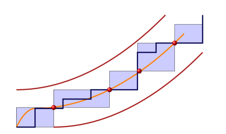
Figure 1: The idea of the proof of the upper bound in Theorem 2.10. The rectangles are defined using the the partition points (the circles). They are disjoint and inside the $\varepsilon-$ neighborhood, so any polymer chain inside those rectangles is inside the neighborhood.

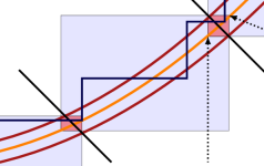
Figure 2: The idea of the proof of the lower bound in Theorem 2.10. The diagonal lines are the $\|\gamma(t_{i})\|$ hyperplanes. The extra error (compared to proof of the lower bound) comes from the common small rectangles with the hyperplanes as diagonals. That error can become small if the $\varepsilon$-neighborhood is sufficiently narrow.

The remaining proof is about the lower bound. A word on the arrangement of the proof: The first part of what follows is used to specify an $\varepsilon_{0}>0$ such that certain macroscopic uniformity and continuity conditions are satisfied (here we use the fact that $\gamma$ is Lipschitz). After $\varepsilon_{0}$ is specified we define a neighborhood $\mathcal{N}_{\varepsilon}$ for $\varepsilon<\varepsilon_{0}$ and work microscopically to bound the quenched probabilities. That part of the proof works for any $\varepsilon<\varepsilon_{0}$. The need for the conditions that specify $\varepsilon_{0}$ become apparent after taking the limits (calculations (2.75)-(2.77)).

Fix $L\in\mathbb{R}_{+}$ and let $\gamma:[0,1]\to\mathbb{R}^{d}_{+}$ be a curve such that each coordinate $\gamma_{j}(t)$, $1\leq j\leq d$, is non-decreasing and $L$-Lipschitz. An immediate consequence is that $0\leq\gamma_{j}^{\prime}(t)\leq L$ for all $t$ where the derivative is defined. Since $\gamma$ is Lipschitz, the difference quotients are bounded

$$\Big{|}\frac{\gamma_{j}(x)-\gamma_{j}(y)}{x-y}\Big{|}\leq L\quad x,y\in[0,1],\,\,1\leq j\leq d.$$ (2.69)

Let $\varepsilon^{\prime}>0$ and restrict the limiting point-to-point free energy $p(\cdot)$ on the set $A_{L}=\{\|\mathbf{u}\|_{1}\leq dL\}$. The function $p$ is uniformly continuous on $A_{L}$, so it admits a modulus of continuity and we can specify $\delta^{\prime}>0$ so that

$$\sup_{\begin{subarray}{c}\|\mathbf{u}-\mathbf{v}\|_{1}<\delta^{\prime}\\ \mathbf{u},\mathbf{v}\in A_{L}\end{subarray}}|p(\mathbf{u})-p(\mathbf{v})|<\varepsilon^{\prime}.$$ (2.70)

For a given $\varepsilon^{\prime}>0$, denote by $\Omega(\varepsilon^{\prime})$ the supremum of $\delta^{\prime}>0$ such that (2.70) holds. As soon as $\delta^{\prime}$ is specified, define a partition

$$\lambda_{M}(\varepsilon^{\prime})=\{0=t_{1}<t_{2}<\cdots<t_{M}=1\}$$

so that for all partition points $t_{i}$, the derivative $\gamma^{\prime}(t_{i})$ exists, and so that for all $1\leq i\leq M$ and $1\leq j\leq d$,

$$\Big{|}\frac{\gamma_{j}(t_{i+1})-\gamma_{j}(t_{i})}{t_{i+1}-t_{i}}-\gamma_{j}^{\prime}(t_{i})\Big{|}<\frac{\delta^{\prime}}{2d}.$$ (2.71)

Pick $\varepsilon>0$ and $\mathcal{N}_{\varepsilon}(\gamma)$ an $\varepsilon-$neighborhood of $\gamma$ in the $\|\cdot\|_{1}$ norm. Assume $\varepsilon$ is small enough so that

$$\varepsilon<\varepsilon_{0}=\min\Big{\{}\Omega(\varepsilon^{\prime}/2M),\,\varepsilon^{\prime}/2M,\,\min_{1\leq i\leq M-1}\{\|\gamma(t_{i+1})-\gamma(t_{i})\|_{1}/M\}\Big{\}}.$$ (2.72)

For any vector $\mathbf{u}\in\mathbb{R}^{d}_{+}$ define the hyperplane $H(\mathbf{u})=\{\mathbf{x}\in\mathbb{R}^{d}_{+}:\|\mathbf{x}\|_{1}=\|\mathbf{u}\|_{1}\}$ and the positive half-space $H_{+}(\mathbf{u})=\{\mathbf{x}\in\mathbb{R}^{d}_{+}:\|\mathbf{x}\|_{1}\geq\|\mathbf{u}\|_{1}\}$. We also denote $H_{-}(\mathbf{u})=H_{+}^{c}(\mathbf{u})$.

Observe that there exist vectors $\{\mathbf{a}^{j}_{i}\}_{1\leq i\leq M-1}^{j=1,2}$ such that for each $i,j$ the following hold:

1. $\mathbf{a}_{i}^{1}\leq\gamma(t_{i})\leq\mathbf{a}_{i}^{2},\quad 1\leq i\leq M$,

2. $\|\gamma(t_{i})-\mathbf{a}_{i}^{j}\|_{1}=\varepsilon,\quad j=1,2$,

3. $R(\lfloor{n\mathbf{a}_{i}^{1}}\rfloor,\lfloor{n\mathbf{a}_{i+1}^{2}}\rfloor)\supseteq n\mathcal{N}_{\varepsilon}(\gamma{[t_{i},t_{i+1})})\cap H_{+}(\lfloor{n\gamma(t_{i})}\rfloor)\cap H_{-}(\lfloor{n\gamma(t_{i+1})}\rfloor)=\mathcal{H}^{n}_{i}.$

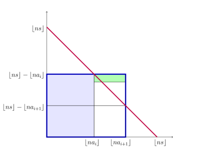
Figure 2: The partition function in the thick-set square bounds from above the product of the partition functions of the shaded parts. This is used in the proof of Theorem 3.3.

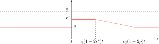
Figure 2: Density profile $\rho(x,t)$ in the two-phase ($c_{1}>c_{2}$) TASEP when we start from constant initial configurations $\rho_{0}(x)\equiv\rho\in(0,\rho^{*}).$

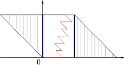
Figure 2: A possible microscopic path described in Lemma 5.6. The path has to stay in the unshaded region.

The set $\mathcal{H}^{n}_{i}$ is the set between two consecutive hyperplanes and in $n\mathcal{N}_{\varepsilon}$ (see Figure 2). Denote the partition function $\mathcal{H}^{n}_{i}$ by

$$Z_{\mathcal{H}_{i}^{n}}=\sum_{x^{(i)}\in\mathcal{H}_{i}^{n}}\prod_{j=\lfloor{n\gamma(t_{i})}\rfloor+1}^{\lfloor{n\gamma(t_{i+1})}\rfloor}e^{\beta\omega(x^{(i)}_{j})},$$

where $x^{(i)}$ is any up-right path living in $\mathcal{H}^{n}_{i}$.

Define $\Pi_{i,n\varepsilon}^{1}=\{x_{0,n\varepsilon}:x_{0}=\lfloor{n\mathbf{a}_{i}^{1}}\rfloor\}$, and $\Pi_{i,n\varepsilon}^{2}=\{x_{0,n\varepsilon}:x_{0}\in H(\lfloor{n\gamma(t_{i})}\rfloor),x_{n\varepsilon}=\lfloor{n\mathbf{a}_{i}^{2}}\rfloor\}$, the set of all path of length $n\varepsilon$ that start from $\lfloor{n\mathbf{a}_{i}^{j}}\rfloor$ and the set of paths that start somewhere on the hyperplane $H(\lfloor{n\gamma(t_{i})}\rfloor)$ and end after $\lfloor{n\varepsilon}\rfloor$ + O(1) steps at $\lfloor{n\mathbf{a}_{i}^{2}}\rfloor$, respectively. The error comes from the integer parts, but is eventually immaterial so we ignore it for convenience.

Observe that any polymer chain that starts at $\lfloor{n\mathbf{a}^{1}_{i}}\rfloor$ and ends at $\lfloor{n\mathbf{a}^{2}_{i+1}}\rfloor$ has to cross the hyperplanes $H(\lfloor{n\gamma(t_{i})}\rfloor)$ and $H(\lfloor{n\gamma(t_{i+1})}\rfloor)$ at some points $\alpha$ and $\beta$ respectively.

The three conditions, along with (2.72) guarantee that $\bigcup_{1\leq i\leq M-1}R(\lfloor{n\mathbf{a}_{i}^{1}}\rfloor,\lfloor{n\mathbf{a}_{i+1}^{2}}\rfloor)\supseteq n\mathcal{N}_{\varepsilon}(\gamma)$ while the common $R(\lfloor{n\mathbf{a}_{i}^{1}}\rfloor,\lfloor{n\mathbf{a}_{i}^{2}}\rfloor)$ (the red-shaded rectangles in Figure 2) are pairwise disjoint and “small”, in the sense of the following bound:

$$Z {}_{\lfloor{n\mathbf{a}_{i}^{1}}\rfloor,\lfloor{n\mathbf{a}_{i+1}^{2}}\rfloor}=\sum_{(\alpha,\beta)\in H(\lfloor{n\gamma(t_{i})}\rfloor)\times H(\lfloor{n\gamma(t_{i+1})}\rfloor)}Z_{\lfloor{n\mathbf{a}_{i}^{1}}\rfloor,\alpha}Z_{\alpha,\beta}Z_{\beta,\lfloor{n\mathbf{a}_{i+1}^{2}}\rfloor}$$

$$\geq\sum_{(\alpha,\beta)\in H(\lfloor{n\gamma(t_{i})}\rfloor)\times H(\lfloor{n\gamma(t_{i+1})}\rfloor)}Z_{\alpha,\beta}\min_{x_{0,n\varepsilon}\in\Pi_{i,n\varepsilon}^{1}}\prod_{j=1}^{\lfloor{n\varepsilon}\rfloor}e^{\beta\omega(x_{j})}\min_{x_{0,n\varepsilon}\in\Pi_{i+1,n\varepsilon}^{2}}\prod_{j=1}^{\lfloor{n\varepsilon}\rfloor}e^{\beta\omega(x_{j})}$$

$$\geq Z_{\mathcal{H}^{n}_{i}}\min_{x_{0,n\varepsilon}\in\Pi_{i,n\varepsilon}^{1}}\prod_{j=1}^{\lfloor{n\varepsilon}\rfloor}e^{\beta\omega(x_{j})}\min_{x_{0,n\varepsilon}\in\Pi_{i+1,n\varepsilon}^{2}}\prod_{j=1}^{\lfloor{n\varepsilon}\rfloor}e^{\beta\omega(x_{j})}.$$ (2.73)

Hence we can bound the probabilities

$$Q^{\omega}_{n}\{x_{0,n} \in n\mathcal{N}_{\varepsilon}(\gamma)\}=Q_{n}^{\omega}\{x_{0,n}\in\cup_{i=1}^{M-1}\mathcal{H}^{n}_{i}\}$$

$$=(Z_{n})^{-1}{\sum_{x_{0,n}\in\mathcal{N}_{\varepsilon}(\gamma)}\prod_{j=1}^{n}e^{\beta\omega(x_{j})}}$$

$$\leq(Z_{n})^{-1}\prod_{i=1}^{M-1}Z_{\mathcal{H}^{n}_{i}}$$

$$\leq(Z_{n})^{-1}\prod_{i=1}^{M}Z_{\lfloor{n\mathbf{a}_{i}^{1}}\rfloor,\lfloor{n\mathbf{a}_{i+1}^{2}}\rfloor}$$

$$\phantom{xxxxxxxx}\times\Big{(}\min_{x_{0,n\varepsilon}\in\Pi_{i,n\varepsilon}^{1}}\prod_{j=1}^{\lfloor{n\varepsilon}\rfloor}e^{\beta\omega(x_{j})}\times\min_{x_{0,n\varepsilon}\in\Pi_{i+1,n\varepsilon}^{2}}\prod_{j=1}^{\lfloor{n\varepsilon}\rfloor}e^{\beta\omega(x_{j})}\Big{)}^{-1}.$$ (2.74)

We are going to take logarithms on both sides of (2.74). On the right-hand side, we have $\log\min_{x_{0,n\varepsilon}\in\Pi_{i,n\varepsilon}^{1}}\prod_{j=1}^{\lfloor{n\varepsilon}\rfloor}e^{-\beta|\omega(x_{j})|}$ which is the first passage percolation time of $n\varepsilon$ steps if the weights were negative (so the negative of last passage percolation time if the weights where positive) with limiting constant $c_{-|\omega|}(\varepsilon)$.

Then, we conclude

$$-\varlimsup_{n\rightarrow\infty}n^{-1}\log Q^{\omega}_{n}\{x_{0,n}\in n\mathcal{N}_{\varepsilon}(\gamma)\} \geq p(d^{-1}\mathbf{1})-\sum_{i=1}^{M-1}p(\mathbf{a}^{2}_{i+1}-\mathbf{a}^{1}_{i})+2Mc_{-|\omega|}(\varepsilon)$$

$$\geq p(d^{-1}\mathbf{1})-\sum_{i=1}^{M-1}p(\mathbf{a}^{2}_{i+1}-\mathbf{a}^{1}_{i})+2\varepsilon^{\prime}d^{-1}c_{-|\omega|}(\mathbf{1})$$

$$\geq p(d^{-1}\mathbf{1})-\sum_{i=1}^{M-1}p(\gamma(t_{i+1})-\gamma(t_{i}))-C\varepsilon^{\prime}$$ (2.75)

$$=p(d^{-1}\mathbf{1})-\sum_{i=1}^{M-1}p\Big{(}\frac{\gamma(t_{i+1})-\gamma(t_{i})}{t_{i+1}-t_{i}}\Big{)}(t_{i+1}-t_{i})-C\varepsilon^{\prime}$$ (2.76)

$$\geq p(d^{-1}\mathbf{1})-\sum_{i=1}^{M-1}p(\gamma^{\prime}(t_{i}))(t_{i+1}-t_{i})-C\varepsilon^{\prime}.$$ (2.77)

Equation (2.75) is the result of (2.72) and (2.70). Homogeneity of $p$ gives (2.76) and then (2.72) and (2.71) give (2.77). The bound in (2.77) is independent of $\varepsilon$ so letting $\varepsilon\to 0$ does not affect it. To get the result, let the mesh of the partition tend to $0$ and then let $\varepsilon^{\prime}\to 0$. ∎

Chapter 3 The log-gamma Polymer Model

3.1 The model

3.1.1 Introduction and results

In the present chapter, we derive an explicit expression for the upper tail rate function for $\log Z_{\lfloor{n\mathbf{u}}\rfloor}$ in the case of the $1+1$ dimensional log-gamma polymer. The computations are tractable exactly because of the Burke property. More detailed information about the model and basic properties can be found in Section 3.1.2.

The results for the particular $1+1$ dimensional log-gamma model. The distributions of the $\omega$ weights are i.i.d.

$$\omega(i,j)\sim\log Y,\quad\text{ where }Y^{-1}\sim\text{Gamma}(\mu),$$ (3.1)

where the density of the Gamma$(\mu)$ is given by (A.2). For this choice of i.i.d.  weights, denote by

$$M_{\mu}(\xi)=\log\mathbb{E}\big{(}e^{\xi\omega(0,0)}\big{)}=\log\Gamma(\mu-\xi)-\log\Gamma(\mu)$$ (3.2)

the logarithmic moment generating function.

It is convenient for the proof of these results to write the vectors in $\mathbb{R}_{+}^{2}$ using both their coordinates. The main result is an explicit formula for the upper tail large deviation rate function for the logarithm of the partition function.

Theorem 3.1.

Let $r\in\mathbb{R}$ and let $\omega(i,j)$ to be distributed as in (3.1). The function $J_{s,t}(r)$ defined by (2.13) is given by

$$J_{s,t}(r)=\sup_{\xi\in[0,\mu)}\Big{\{}r\xi-\inf_{\xi<\theta<\mu}\bigl{(}tM_{\theta}(\xi)-sM_{\mu-\theta}(-\xi)\bigr{)}\Big{\}}.$$ (3.3)

Remark 3.2.

While the symmetry of $J_{s,t}$ is clear by definition (2.13), it is not immediately obvious from (3.3). From the proof of the theorem for $s\leq t$ one can check that we can restrict the set where the inner infimum is taken to $\theta\in[(\mu+\xi)/2,\mu)$. Under the assumption that $s\geq t$ it is easy to check that the infimum is now attainable for $\theta\in(\xi,(\mu+\xi)/2]$. If $s\leq t$ and $\theta_{0}$ gives the infimum $\gamma_{*}$, it is easy to check that interchanging the roles of $s,t$ will give the same infimum $\gamma_{*}$ at $\theta_{1}=\mu+\xi-\theta_{0}$. These symmetries will be explained in detail in the proof the theorem.

The next result is about the free-endpoint case.

Theorem 3.3.

Let $s>0$, $r\in\mathbb{R}$. The large deviation rate function (2.14), for $\beta=1$ is

$$-\lim_{n\rightarrow\infty}n^{-1}\log\mathbb{P}\{\log Z_{\lfloor{ns}\rfloor}\geq nr\}=J_{s/2,s/2}(r)$$ (3.4)

where $J_{s,t}(r)$ is given by (3.3).

.

3.1.2 The model and the Burke property

For the rest of this chapter we also the the parameter $\beta$ to equal $1$. Henceforth we adopt the multiplicative notation for the polymer measure. It is also convenient to adjust the notation for the partition functions and redefine the rate functions:

On each site $(i,j)$ of $\mathbb{Z}_{+}^{2}$ we assign weights $Y_{i,j}$. For any $(k,\ell)<(m,n)$ define the partition function for paths that start from $(k,\ell)$ and whose endpoint is constrained to be $(m,n)$, by

$$Z_{(k,\ell),(m,n)}=\sum_{x_{\cdot}\in\Pi_{(k,l),(m,n)}}\prod_{j=k+\ell+1}^{m+n}Y_{x_{j}},$$ (3.5)

where $\Pi_{(k,l),(m,n)}$ is the collection of up-right paths $x_{\cdot}=(x_{j})_{k+\ell\leq j\leq m+n}$ inside the rectangle $R_{k,\ell}^{m,n}=\{k,k+1,...,m\}\times\{\ell,...,n\}$ that go from $(k,\ell)$ to $(m,n)$: $x_{k+\ell}=(k,\ell)$, $x_{m+n}=(m,n)$. We adopt the convention that $Z_{(k,\ell),(m,n)}$ does not include the weight at the starting point. In the case that the weight at the starting point needs to be considered we also define

$$Z^{\square}_{(k,\ell),(m,n)}=\sum_{x_{\cdot}\in\Pi_{(k,l),(m,n)}}\prod_{j=k+\ell}^{m+n}Y_{x_{j}}=Y_{k,\ell}Z_{(k,\ell),(m,n)},$$ (3.6)

If a value is needed, then assume that $Z_{k,\ell,(k,\ell)}=1.$ In the special case where $(k,\ell)=(0,0)$ we omit the subscript from the above notation and we also set $Y_{0,0}=1.$

We assign distinct weight distributions on the boundaries $\mathbb{N}\times\{0\}$, $\{0\}\times\mathbb{N}$ and in the bulk $\mathbb{N}^{2}$. To emphasize this, the symbols $U$ and $V$ will denote the weights on the horizontal and vertical boundary respectively:

$$U_{i,0}=Y_{i,0}\quad\textrm{and}\quad V_{0,j}=Y_{0,j}.$$ (3.7)

Our results depend on the explicit distribution of the weights; all weights are reciprocals of gamma variables. To be precise, here are the assumptions on the distributions:

Assumption 3.4.

Let $0<\theta<\mu<\infty$. We assume that the weights $\{U_{i,0},V_{0,j},Y_{i,j}:i,j\in\mathbb{N}\}$ are independent with distributions

$$U_{i,0}^{-1}\sim\text{Gamma}(\theta),V_{0,j}^{-1}\sim\text{Gamma}(\mu-\theta),\textrm{ and }Y_{i,j}^{-1}\sim\text{Gamma}(\mu).$$ (3.8)

Given the initial weights $\{U_{i,0},V_{0,j},Y_{i,j}:i,j\in\mathbb{N}\}$ and starting from the lower left corner of $\mathbb{N}^{2}$, define inductively for $(i,j)\in\mathbb{N}^{2}$

$$U_{i,j}=Y_{i,j}\Big{(}1+\frac{U_{i,j-1}}{V_{i-1,j}}\Big{)},\,V_{i,j}=Y_{i,j}\Big{(}1+\frac{V_{i-1,j}}{U_{i,j-1}}\Big{)}\,\textrm{and }X_{i-1,j-1}=\Big{(}\frac{1}{U_{i,j-1}}+\frac{1}{V_{i-1,j}}\Big{)}^{-1}.$$ (3.9)

The partition function for the model with the boundary condition is denoted by $Z^{(\theta)}_{m,n}$ satisfies

$$Z^{(\theta)}_{m,n}=Y_{m,n}(Z^{(\theta)}_{m-1,n}+Z^{(\theta)}_{m,n-1})\textrm{ for }(m,n)\in\mathbb{N}^{2}$$ (3.10)

and one can check inductively that

$$U_{m,n}=\frac{Z^{(\theta)}_{m,n}}{Z^{(\theta)}_{m-1,n}}\,\,\textrm{ and }\,\,V_{m,n}=\frac{Z^{(\theta)}_{m,n}}{Z^{(\theta)}_{m,n-1}}.$$ (3.11)

Equations (3.10) and (3.11) are also valid for $Z^{\square}(m,n)$ since the weight at the origin is canceled from the equations.

The key result that allows explicit calculations for this model is the Burke-type Theorem 3.3 in [29].

Let $z_{\cdot}=(z_{k})_{k\in\mathbb{Z}}$ be a nearest-neighbor down-right path in $\mathbb{Z}^{2}_{+}$, that is, $z_{k}\in\mathbb{Z}^{2}_{+}$ and $z_{k}-z_{k-1}=e_{1}$ or $-e_{2}$. Denote the undirected edges of the path by $f_{k}=\{z_{k-1},z_{k}\}$ and let

$$T_{f_{k}}=\begin{cases}U_{z_{k}}&\text{if }f_{k}\text{ is a horizontal edge}\\ V_{z_{k-1}}&\text{if }f_{k}\text{ is a vertical edge}.\end{cases}$$

Let the lower left interior of the path be the vertex set $\mathcal{I}=\{(i,j)\in\mathbb{Z}^{2}_{+}:\exists\,m\text{ so that }(i+m,j+m)\in\{z_{k}\}\}.$

Recall the definition of $X_{i,j}$ from (3.9).

Theorem 3.5 ([29]-Burke Property).

Under the assumption (3.8), and for any down-right path $(z_{k})_{k\in\mathbb{Z}}$ in $\mathbb{Z}_{+}^{2}$, the variables $\{T_{f_{k}},X_{z}:k\in\mathbb{Z},z\in\mathcal{I}\}$ are mutually independent with marginal distributions

$$U^{-1}\sim\text{Gamma}(\theta),V^{-1}\sim\text{Gamma}(\mu-\theta),\textrm{ and }X^{-1}\sim\text{Gamma}(\mu).$$ (3.12)

From this, one can compute

$$\mathbb{E}(\log Z^{(\theta)}_{m,n})=m\mathbb{E}(\log U)+n\mathbb{E}(\log V)=-m\Psi_{0}(\theta)-n\Psi_{0}(\mu-\theta).$$ (3.13)

In [29] a law of large numbers is proved for the limiting free energy in the case of no boundary weights. Let $(s,t)\in\mathbb{R}^{2}_{+}$ and observe that there exists a unique $\theta=\theta_{s,t}\in(0,\mu)$ such that $t\Psi_{1}(\mu-\theta)=s\Psi_{1}(\theta).$ Define

$$p_{\mu}(s,t)=-(s\Psi_{0}(\theta_{s,t})+t\Psi_{0}(\mu-\theta_{s,t})).$$ (3.14)

For the model without boundaries with $Y^{-1}_{i,j}\sim\textrm{Gamma}(\mu),\,i\geq 0,j\geq 0$, the limiting free energies can be evaluated explicitly to be

$$\lim_{n\rightarrow\infty}n^{-1}\log Z_{\lfloor{ns}\rfloor,\lfloor{nt}\rfloor}=p_{\mu}(s,t)\quad\mathbb{P}-a.s.$$ (3.15)

and

$$\lim_{n\rightarrow\infty}n^{-1}\log Z^{\operatorname{tot}}_{\lfloor{ns}\rfloor}=-s\Psi_{0}(\mu/2)\quad\mathbb{P}-a.s.$$ (3.16)

3.2 Continuity of the rate function on the boundary

The logarithmic moment generating function of the bulk weights $\log Y_{i,j}\sim$ $-\log$ Gamma$(\mu)$ is

$$M_{\mu}(\xi)=\log\mathbb{E}\bigl{(}e^{\xi\log Y}\bigr{)}=\begin{cases}\log\Gamma(\mu-\xi)-\log\Gamma(\mu),&\xi<\mu\\ \infty,&\xi\geq\mu.\end{cases}$$

Its convex dual is the Cramér rate function (recall (2.8)) $I_{\mu}$ of this distribution, given by

$$I_{\mu}(r) =-r\Psi^{-1}_{0}(-r)-\log\Gamma(\Psi^{-1}_{0}(-r))+\mu r+\log\Gamma(\mu),\quad r\in\mathbb{R}.$$ (3.17)

From Theorem 2.5 we know that the rate function for the model with i.i.d weights is continuous on the boundary, and in this case, its value equals the Cramér rate function for the sum of i.i.d. weights with inverse Gamma$(\mu)$ distribution.

The rate function on the boundary is given by

$$J_{0,x}(r)=J_{x,0}(r)=\begin{cases}xI_{\mu}(rx^{-1}),&\quad r\geq-x\Psi_{0}(\mu),\,x>0\\ r\mu,&\quad r\geq 0,\,x=0\\ 0,&\quad r<-x\Psi_{0}(\mu),\,x\geq 0.\end{cases}$$ (3.18)

For the second branch of (3.18) we used

$$\lim_{x\searrow 0}x\log\Gamma(\Psi_{0}^{-1}(-rx^{-1}))=0,\quad r>0.$$ (3.19)

Note that $J_{0,0}(r)=r\mu$ as given by (2.15). (Here $\mu=x_{\infty}$). One can also interpret the second branch as the large deviation rate function for a single $\log Y$ random variable, where $Y^{-1}\sim$ Gamma($\mu$).

The strong law of large numbers for the limiting constant of the free energy from (3.15) and continuity of $J$ give the support described in the theorem. The fact that $J$ is strictly increasing for $r\geq p_{\mu}(s,t)$ can follow independently after finding the rate function explicitly in Theorem 3.3.

3.3 Exact point-to-point rate function

Lemma 3.6 (Varadhan’s lemma).

Let $Z_{\lfloor{ns}\rfloor,\lfloor{nt}\rfloor}$ the partition function given by (3.5) with weights $Y$ such that $Y^{-1}\sim\text{Gamma}(\mu)$. Also let $J_{s,t}(r)$ the upper tail large deviation for $\log Z_{\lfloor{ns}\rfloor,\lfloor{nt}\rfloor}$. Then for $0\leq\xi<\mu$

$$\lim_{n\to\infty}n^{-1}\log\mathbb{E}e^{\xi\log Z_{\lfloor{ns}\rfloor,\lfloor{nt}\rfloor}}=\sup_{r\in\mathbb{R}}\{r\xi-J_{s,t}(r)\}=J^{*}_{s,t}(\xi).$$

Proof.

Let $\gamma_{\inf}=\varliminf_{n\to\infty}n^{-1}\log\mathbb{E}e^{\xi\log Z_{\lfloor{ns}\rfloor,\lfloor{nt}\rfloor}}$ and $\gamma_{sup}=\varlimsup_{n\to\infty}n^{-1}\log\mathbb{E}e^{\xi\log Z_{\lfloor{ns}\rfloor,\lfloor{nt}\rfloor}}.$ First an exponential Chebychev argument for a lower bound:

$$n^{-1}\log\mathbb{P}\{\log Z_{\lfloor{ns}\rfloor,\lfloor{nt}\rfloor}\geq nr\}\leq-\xi r+n^{-1}\log\mathbb{E}e^{\xi\log Z_{\lfloor{ns}\rfloor,\lfloor{nt}\rfloor}}.$$

By letting $n\to\infty$ on a suitable subsequence we get that for all $r\in\mathbb{R}$

$$\gamma_{\inf}\geq\xi r-J_{s,t}(r).$$

Optimizing over $r$ we get $\gamma_{\inf}\geq J_{s,t}^{*}(\xi).$

For the upper bound, first note that there exists $\alpha>1$ such that $\alpha\xi<\mu$,

$$\sup_{n}\Big{(}\mathbb{E}e^{\alpha\xi\log Z_{\lfloor{ns}\rfloor,\lfloor{nt}\rfloor}}\Big{)}^{1/n}<\infty.$$ (3.20)

To see this, distinguish cases where $\alpha\xi<1$ or otherwise. For $\alpha\xi<1$,

$$\Big{(}\mathbb{E}e^{\alpha\xi\log Z_{\lfloor{ns}\rfloor,\lfloor{nt}\rfloor}}\Big{)}^{1/n} =\Big{(}\mathbb{E}\Big{(}\sum_{x\in\Pi(\lfloor{ns}\rfloor,\lfloor{nt}\rfloor)}\prod_{i=1}^{\lfloor{ns}\rfloor+\lfloor{nt}\rfloor}Y_{x_{j}}\Big{)}^{\alpha\xi}\Big{)}^{1/n}$$

$$\leq\Big{(}\sum_{x\in\Pi(\lfloor{ns}\rfloor,\lfloor{nt}\rfloor)}\prod_{i=1}^{\lfloor{nt}\rfloor+\lfloor{ns}\rfloor}\mathbb{E}Y^{\alpha\xi}\Big{)}^{1/n}$$

$$\leq e^{F(s,t)+o(1)}(M_{\mu}(\alpha\xi))^{t+s}.$$

For $\alpha\xi\geq 1$, we use Jensen’s inequality. Let N denote the number of paths.

$$\Big{(}\mathbb{E}e^{\alpha\xi\log Z_{\lfloor{ns}\rfloor,\lfloor{nt}\rfloor}}\Big{)}^{1/n} =\Big{(}\mathbb{E}\Big{(}\sum_{x\in\Pi(\lfloor{ns}\rfloor,\lfloor{nt}\rfloor)}\prod_{i=1}^{\lfloor{ns}\rfloor+\lfloor{nt}\rfloor}Y_{x_{j}}\Big{)}^{\alpha\xi}\Big{)}^{1/n}$$

$$\leq\Big{(}N^{\alpha\xi}\sum_{x\in\Pi(\lfloor{ns}\rfloor,\lfloor{nt}\rfloor)}\prod_{i=1}^{\lfloor{nt}\rfloor+\lfloor{ns}\rfloor}\mathbb{E}Y^{\alpha\xi}\Big{)}^{1/n}$$

$$\leq e^{\alpha\xi F(s,t)+O(1)}(M_{\mu}(\alpha\xi))^{t+s}.$$

Now, we can show that

$$\lim_{r\to\infty}\varlimsup_{n\to\infty}n^{-1}\log\mathbb{E}\Big{(}e^{\xi\log Z_{\lfloor{ns}\rfloor,\lfloor{nt}\rfloor}}\mathbf{1}\{\log Z_{\lfloor{ns}\rfloor,\lfloor{nt}\rfloor}\geq nr\}\Big{)}=-\infty.$$ (3.21)

Using Hölder’s inequality,

$$n^{-1}\log\mathbb{E}\Big{(} e^{\xi\log Z_{\lfloor{ns}\rfloor,\lfloor{nt}\rfloor}}\mathbf{1}\{\log Z_{\lfloor{ns}\rfloor,\lfloor{nt}\rfloor}\geq nr\}\Big{)}$$

$$\leq\alpha^{-1}\log\sup_{n}(\mathbb{E}e^{\alpha\xi\log Z_{\lfloor{ns}\rfloor,\lfloor{nt}\rfloor}})^{1/n}+\frac{\alpha-1}{\alpha}n^{-1}\log\mathbb{P}\{\log Z_{\lfloor{ns}\rfloor,\lfloor{nt}\rfloor}\geq nr\}.$$

Taking a limit $n\to\infty$ we conclude

$$\varlimsup_{n\to\infty}n^{-1}\log\mathbb{E}\Big{(}e^{\xi\log Z_{\lfloor{ns}\rfloor,\lfloor{nt}\rfloor}}\mathbf{1}\{\log Z_{\lfloor{ns}\rfloor,\lfloor{nt}\rfloor}\geq nr\}\Big{)}\leq C-\frac{\alpha-1}{\alpha}J_{s,t}(r).$$ (3.22)

Letting $r$ to $\infty$ concludes the proof, since $J_{s,t}(r)$ is a non-constant increasing convex function.

To establish an upper bound let $\delta>0$ and partition $\mathbb{R}$ so that for $i\in\mathbb{Z}$, $r_{i}=i\delta$. Then for any $m$

$$n^{-1}\log\Big{(}\mathbb{E}e^{\xi\log Z_{\lfloor{ns}\rfloor,\lfloor{nt}\rfloor}}\Big{)} =n^{-1}\log\Big{(}\sum_{i=-\infty}^{\infty}\mathbb{E}e^{\xi\log Z_{\lfloor{ns}\rfloor,\lfloor{nt}\rfloor}}\mathbf{1}\{nr_{i}\leq\log Z_{\lfloor{ns}\rfloor,\lfloor{nt}\rfloor}<nr_{i+1}\}\Big{)}$$

$$\leq n^{-1}\log\Big{(}\sum_{i=-m}^{m}e^{n\xi r_{i+1}}\mathbb{P}\{\log Z_{\lfloor{ns}\rfloor,\lfloor{nt}\rfloor}\geq nr_{i}\}$$

$$\phantom{xxxxxxx}+e^{n\xi r_{-m}}+\mathbb{E}\Big{(}e^{\xi\log Z_{\lfloor{ns}\rfloor,\lfloor{nt}\rfloor}}\mathbf{1}\{\log Z_{\lfloor{ns}\rfloor,\lfloor{nt}\rfloor}\geq nr_{m}\}\Big{)}\Big{)}$$ (3.23)

A limit along a suitable subsequence yields

$$\gamma_{\sup} \leq\max\big{\{}\max_{-m\leq i\leq m}\{\xi r_{i+1}-J_{s,t}(r_{i})\},\xi r_{-m},C-\frac{\alpha-1}{\alpha}J_{s,t}(r_{m})\}\big{\}}$$

$$\leq\max\{\sup_{r}\{\xi r-J_{s,t}(r)\}-\delta\xi,\xi r_{-m},C-\frac{\alpha-1}{\alpha}J_{s,t}(r_{m})\}\big{\}}$$

To finish the proof, let $\delta\to 0$ and $m\to\infty$. ∎

An immediate consequence is that $\log Z^{\square}$ and $\log Z$ have the same rate functions. This follows from having the same convex dual for $0\leq\xi<\mu$ (for $\xi\geq\mu$ both rate functions are $\infty$):

$$\lim_{n\to\infty}n^{-1}\log\mathbb{E}e^{\xi\log Z^{\square}_{\lfloor{ns}\rfloor,\lfloor{nt}\rfloor}} =\lim_{n\to\infty}n^{-1}\log\mathbb{E}e^{\xi\log Z_{\lfloor{ns}\rfloor,\lfloor{nt}\rfloor}+\xi\log Y_{1,1}}$$

$$=J^{*}_{s,t}(\xi)+\lim_{n\to\infty}n^{-1}\log\mathbb{E}Y_{1,1}^{\xi}$$

$$=J^{*}_{s,t}(\xi).$$

We are using this fact in the remaining part of the section without alerting the reader.

For what follows we need some notational conventions. Assume the polymer lives in the rectangle $\{0,\dotsc,\lfloor{ns}\rfloor\}\times\{0,\dotsc,\lfloor{nt}\rfloor\}$ and let $-\lfloor{nt}\rfloor\leq k\leq\lfloor{ns}\rfloor$. Let $Y_{0,0}=1$ and define

$$\eta_{k}=\begin{cases}\displaystyle\prod_{j=-k+1}^{\lfloor{nt}\rfloor}V_{0,j}^{-1},&\text{ for }-\lfloor{nt}\rfloor\leq k\leq-1,\\ \eta_{-1},&k=0\\ \displaystyle\eta_{0}\prod_{i=1}^{k}U_{i,0},&\text{ for }0<k\leq\lfloor{ns}\rfloor,\\ \end{cases}$$ (3.24)

and

$$\mathbf{k}=\begin{cases}(1,-k),&-\lfloor{nt}\rfloor\leq k\leq-1,\\ (1,1),&k=0,\\ (k,1),&0<k\leq\lfloor{ns}\rfloor,\end{cases}\quad\text{and}\quad\lfloor{n\mathbf{a}}\rfloor=\begin{cases}(1,\lfloor{-na}\rfloor),&-t\leq a<0,\\ (1,1),&a=0,\\ (\lfloor{na}\rfloor,1),&0<a\leq s.\end{cases}$$ (3.25)

It is going to be notationally convenient to assume that $k=\lfloor{na}\rfloor$ for some $a\in[-t,s]$. Whenever this happens, we identify $\mathbf{k}=\lfloor{n\mathbf{a}}\rfloor$ and we assume that $n$ is large enough so that $\lfloor{na}\rfloor\neq 0$. When we take the limit as $n\rightarrow\infty$ to compute the various rate functions, we will need a continuous (and scaled) version of (3.25). For this reason we abuse this notation by writing

$$\mathbf{a}=\lim_{n\rightarrow\infty}n^{-1}\lfloor{n\mathbf{a}}\rfloor=\begin{cases}(0,-a),&-t\leq a<0,\\ (0,0),&a=0\\ (a,0),&0<a\leq s.\end{cases}$$ (3.26)

Observe that for all $a\in[-t,s]$, the r.v. $\log\eta_{\lfloor{na}\rfloor}$ is a sum of independent $\log$-gamma random variables: For $a<0$, $\log\eta_{\lfloor{na}\rfloor}$ is just a sum of i.i.d. $\log$ Gamma$(\mu-\theta)$, the Cramér rate function exists and so are the lower and upper large deviations rate functions.

For $a>0$,

$$\log\eta_{\lfloor{na}\rfloor}=\sum_{j=1}^{\lfloor{nt}\rfloor}\log V_{0,j}^{-1}-\sum_{i=1}^{\lfloor{na}\rfloor}\log U_{i,0}^{-1}.$$

Setting $L_{n}=\sum_{j=1}^{\lfloor{nt}\rfloor}\log V_{0,j}^{-1}$, $Z_{n}=-\sum_{i=1}^{\lfloor{na}\rfloor}\log U_{i,0}^{-1}$, we appeal to Lemma 2.14 so the upper large deviation rate function

$$-\lim_{n\rightarrow\infty}n^{-1}\log\mathbb{P}\{\log\eta_{\lfloor{na}\rfloor}\geq nr\}=\kappa_{a}(r)$$ (3.27)

exists and is convex and continuous. With these definitions we can have the following computational lemma that we are using throughout.

Lemma 3.7.

Fix $a\in[-t,s]$ and let $\kappa_{a}(r)$ defined by (3.27). Then

$$\kappa^{*}_{a}(\xi)=\begin{cases}(t+a)\big{(}\log\Gamma(\mu-\theta+\xi)-\log\Gamma(\mu-\theta)\big{)},\quad-t\leq a\leq 0,\,\,\xi\geq 0,\vspace{0.1 in}\\ t\big{(}\log\Gamma(\mu-\theta+\xi)-\log\Gamma(\mu-\theta)\big{)}+a\big{(}\log\Gamma(\theta-\xi)-\log\Gamma(\theta)\big{)}\\ \phantom{xxxxxxxxxxxxxxxxxxxxxxxxxxxxxxxxx}0<a\leq s,\,\,0\leq\xi<\theta,\\ \infty,\phantom{xxxxxxxxxxxxxxxxxxxxxxxxxxxxxx1}\text{otherwise}.\end{cases}$$ (3.28)

Proof.

Fix $a\in[-t,s].$ For $-t\leq a\leq 0$, the first branch of (3.28) is the logarithmic moment generating function for log-gamma weights. The second branch comes by taking the limiting logarithmic moment generating function for $\xi>0$ of $\eta_{\lfloor{na}\rfloor}$. ∎

Recall (3.25). Let $(a,b)\in[-t,s]^{2}$ and let $m_{\kappa,a}$ and $m_{J,b}$ the zeros of $\kappa_{a}$ and $J_{(s,t)-\mathbf{b}}$ respectively. Define

$$H^{a,b}_{s,t}(r) =\lim_{n\to\infty}n^{-1}\log\mathbb{P}\{\log\eta_{\lfloor{na}\rfloor}+\log Z^{\square}_{\lfloor{n\mathbf{b}}\rfloor,(\lfloor{ns}\rfloor,\lfloor{nt}\rfloor)}\geq nr\}$$

$$=\begin{cases}0,&r<m_{\kappa,a}+m_{J,b}\\ \displaystyle\inf_{m_{\kappa,a}\leq x\leq r-m_{J,b}}\{\kappa_{a}(x)+J_{(s,t)-\mathbf{b}}(r-x)\},&\text{otherwise}.\end{cases}$$ (3.29)

where $\kappa_{a}(x)$ is given by (3.27). The existence of $H^{a,b}_{s,t}(r)$ is established by Lemma 2.14 and continuity in the $b$ argument (when $a,s,t,r$ are fixed) follows directly from the continuity of $J$ in $b$, the fact that $J$ is always finite and that $x$ can be restricted in a compact set. In the case where $a=b$ we define $H^{a}_{s,t}(r)=H^{a,a}_{s,t}(r)$.

Let $s,t>0$, $r\in\mathbb{R}$. Let $\big{\{}U_{i,\lfloor{nt}\rfloor}\big{\}}_{1\leq i\leq\lfloor{ns}\rfloor}$ be the weights as defined by (3.9). Define

$$R_{s}(r)=-\lim_{n\rightarrow\infty}n^{-1}\log\mathbb{P}\Bigg{\{}\sum_{i=1}^{\lfloor{ns}\rfloor}\log U_{i,\lfloor{nt}\rfloor}\geq nr\Bigg{\}}=\begin{cases}sI_{\theta}(rs^{-1}),&\quad r\geq-s\Psi_{0}(\theta),\\ 0,&\quad\text{otherwise},\end{cases}$$ (3.30)

with convex dual

$$R^{*}_{s}(\xi)=\begin{cases}s\log\Gamma(\theta-\xi)-s\log\Gamma(\theta),\quad 0\leq\xi<\theta,\\ \infty,\quad\textrm{otherwise},\end{cases}$$ (3.31)

where we use (A.4) and (3.17) to obtain the first branch.

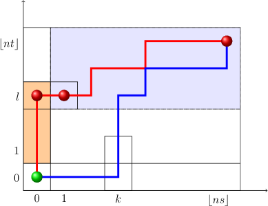
Figure 1: Two possible polymer paths with weights described by (3.8). The shaded parts explain the decomposition of the partition function $Z_{\lfloor{ns}\rfloor,\lfloor{nt}\rfloor}$ needed for Lemma 3.32.

Lemma 3.8.

Let $s,t>0$ , $a\in[-t,s]$ and $r\in\mathbb{R}$. Let (for fixed $s,t,a$) $\kappa_{a}$, $H^{a}_{s,t}$ and $R_{s}$ be defined by (3.27), (3.29) and (3.30). Then

$$R_{s}(r)=\inf_{-t\leq a\leq s}\{H^{a}_{s,t}(r)\}=\inf_{-t\leq a\leq s}\,\,\inf_{m_{\kappa,a}\leq x\leq r-m_{J,a}}\{\kappa_{a}(x)+J_{(s,t)-\mathbf{a}}(r-x)\}.$$ (3.32)

Proof.

We start by decomposing $Z^{(\theta)}_{\lfloor{ns}\rfloor,\lfloor{nt}\rfloor}$ according to the exit point of the polymer path from the boundary:

$$Z^{(\theta)}_{\lfloor{ns}\rfloor,\lfloor{nt}\rfloor} =\sum_{x_{\cdot}\in\Pi_{(0,0),(\lfloor{ns}\rfloor,\lfloor{nt}\rfloor)}}\prod_{j=1}^{\lfloor{ns}\rfloor+\lfloor{nt}\rfloor}Y_{x_{j}}$$

$$=\sum_{\ell=1}^{\lfloor{nt}\rfloor}\bigg{\{}\bigg{(}\prod_{j=1}^{\ell}V_{0,j}\bigg{)}Z^{\square}_{(1,\ell),(\lfloor{ns}\rfloor,\lfloor{nt}\rfloor)}\bigg{\}}+\sum_{k=1}^{\lfloor{ns}\rfloor}\bigg{\{}\bigg{(}\prod_{i=1}^{k}U_{i,0}\bigg{)}Z^{\square}_{(k,1),(\lfloor{ns}\rfloor,\lfloor{nt}\rfloor)}\bigg{\}}.$$ (3.33)

Dividing both sides of (3.33) by $Z^{(\theta)}_{0,\lfloor{nt}\rfloor}=\prod_{j=1}^{\lfloor{nt}\rfloor}V_{0,j}$ and through multiple uses of (3.11), we get

$$\prod_{i=1}^{\lfloor{ns}\rfloor}U_{i,\lfloor{nt}\rfloor} =\sum_{\ell=1}^{\lfloor{nt}\rfloor}\bigg{\{}\bigg{(}\prod_{j=\ell+1}^{\lfloor{nt}\rfloor}V^{-1}_{0,j}\bigg{)}Z^{\square}_{(1,\ell),(\lfloor{ns}\rfloor,\lfloor{nt}\rfloor)}\bigg{\}}$$

$$\phantom{xxxxxxxxxxxxxxxxxx}+\sum_{k=1}^{\lfloor{ns}\rfloor}\bigg{\{}\bigg{(}\prod_{j=1}^{\lfloor{nt}\rfloor}V^{-1}_{0,j}\prod_{i=1}^{k}U_{i,0}\bigg{)}Z^{\square}_{(k,1),(\lfloor{ns}\rfloor,\lfloor{nt}\rfloor)}\bigg{\}}$$

$$=\sum_{\begin{subarray}{c}k=-\lfloor{nt}\rfloor\\[1.0pt] k\neq 0\end{subarray}}^{\lfloor{ns}\rfloor}\eta_{k}Z^{\square}_{\mathbf{k},(\lfloor{ns}\rfloor,\lfloor{nt}\rfloor)}.$$ (3.34)

Since all terms are nonnegative we get the bounds

$$\eta_{k}Z^{\square}_{\mathbf{k},(\lfloor{ns}\rfloor,\lfloor{nt}\rfloor)}\leq\prod_{i=1}^{\lfloor{ns}\rfloor}U_{i,\lfloor{nt}\rfloor}\leq\sum_{k=-\lfloor{nt}\rfloor}^{\lfloor{ns}\rfloor}\eta_{k} Z^{\square}_{\mathbf{k},(\lfloor{ns}\rfloor,\lfloor{nt}\rfloor)}\leq$$

$$\leq\lfloor{n(s+t)}\rfloor\max_{-\lfloor{nt}\rfloor\leq k\leq\lfloor{ns}\rfloor}\eta_{k}Z^{\square}_{\mathbf{k},(\lfloor{ns}\rfloor,\lfloor{nt}\rfloor)}.$$

Take logs of these inequalities to get

$$\log\eta_{k}+\log Z^{\square}_{\mathbf{k},(\lfloor{ns}\rfloor,\lfloor{nt}\rfloor)}\leq\sum_{i=1}^{\lfloor{ns}\rfloor}\log U_{i,\lfloor{nt}\rfloor}\leq\log\bigg{\{}\sum_{k=-\lfloor{nt}\rfloor}^{\lfloor{ns}\rfloor}\eta_{k}Z^{\square}_{\mathbf{k},(\lfloor{ns}\rfloor,\lfloor{nt}\rfloor)}\bigg{\}}$$

$$\phantom{xxxxxxxxxxxxx}\leq\max_{-\lfloor{nt}\rfloor\leq k\leq\lfloor{ns}\rfloor}\big{\{}\log\eta_{k}+\log Z^{\square}_{\mathbf{k},(\lfloor{ns}\rfloor,\lfloor{nt}\rfloor)}\big{\}}+\log(n(s+t)).$$ (3.35)

For any $a\in[-t,s]$,

$$\lim_{n\rightarrow\infty}n^{-1}\log\mathbb{P}\bigg{\{}\sum_{i=1}^{\lfloor{ns}\rfloor} \log U_{i,\lfloor{nt}\rfloor}\geq nr\bigg{\}}$$

$$\geq\lim_{n\rightarrow\infty}n^{-1}\log\mathbb{P}\big{\{}\log\eta_{\lfloor{na}\rfloor}+\log Z^{\square}_{\lfloor{n\mathbf{a}}\rfloor,(\lfloor{ns}\rfloor,\lfloor{nt}\rfloor)}\geq nr\big{\}}$$

$$\geq-H^{a}_{s,t}(r).$$ (3.36)

Equation (3.36) is valid for all $a$, so optimizing over $a\in[-t,s]$ gives

$$\lim_{n\rightarrow\infty}n^{-1}\log\mathbb{P}\bigg{\{}\sum_{i=1}^{\lfloor{ns}\rfloor}\log U_{i,\lfloor{nt}\rfloor}\geq nr\bigg{\}}\geq-\inf_{-t\leq a\leq s}\,\,\inf_{a_{\kappa}\leq x\leq r-a_{J}}\{\kappa_{a}(x)+J_{(s,t)-\mathbf{a}}(r-x)\}.$$

This proves the upper bound in (3.32).

The remaining of the proof is about the lower bound. Let $\varepsilon>0$. Fix a sufficiently small $\delta>0$ and let $-t=a_{0}<a_{1}<\dotsm<a_{q}=0<\dotsm<a_{m}=s$ be a partition of the interval $-[t,s]$ so that $|a_{i+1}-a_{i}|<\delta$. For a given $\xi>0$ assume $\delta=\delta(\varepsilon,\xi)$ is sufficiently small so that $\delta\int_{\mu}^{\mu+\xi}\Psi_{0}(x)\,dx<\varepsilon/4$.

Without loss of generality assume $a_{i}\geq 0$. For any integer $k\in[\lfloor{na_{i}}\rfloor,\lfloor{na_{i+1}}\rfloor]$, we can estimate

$$\mathbb{P} \big{\{}\log\eta_{k}+\log Z^{\square}_{\mathbf{k},(\lfloor{ns}\rfloor,\lfloor{nt}\rfloor)}\geq nr\big{\}}$$

$$\leq\mathbb{P}\bigg{\{}\log\eta_{\lfloor{na_{i+1}}\rfloor}+\log Z^{\square}_{\lfloor{n\mathbf{a}_{i}}\rfloor,(\lfloor{ns}\rfloor,\lfloor{nt}\rfloor)}-\sum_{i=k+1}^{\lfloor{na_{i+1}}\rfloor}\log U_{i,0}-\sum_{j=\lfloor{na_{i}}\rfloor}^{k-1}\log Y_{j,1}\geq nr\bigg{\}}$$ (3.37)

$$\leq\mathbb{P}\big{\{}\log\eta_{\lfloor{na_{i+1}}\rfloor}+\log Z^{\square}_{\lfloor{n\mathbf{a}_{i}}\rfloor,(\lfloor{ns}\rfloor,\lfloor{nt}\rfloor)}\geq n(r-\varepsilon)\big{\}}$$

$$\phantom{xxxxxxxxxxxxxxx}+\mathbb{P}\Bigg{\{}-\sum_{i=k+1}^{\lfloor{na_{i+1}}\rfloor}\log U_{i,0}-\sum_{j=\lfloor{na_{i}}\rfloor}^{k-1}\log Y_{j,1}\geq n\varepsilon\bigg{\}}$$

$$\leq\mathbb{P}\big{\{}\log\eta_{\lfloor{na_{i+1}}\rfloor}+\log Z^{\square}_{\lfloor{n\mathbf{a}_{i}}\rfloor,(\lfloor{ns}\rfloor,\lfloor{nt}\rfloor)}\geq n(r-\varepsilon)\big{\}}$$

$$\phantom{xxxxxxxxxxxxxxx}+e^{-\xi n\varepsilon}\big{(}\mathbb{E}e^{\xi\log U^{-1}}\big{)}^{n(a_{i+1}-k-1)}\big{(}\mathbb{E}e^{\xi\log Y^{-1}}\big{)}^{k-na_{i}-1}$$

$$\leq\mathbb{P}\big{\{}\log\eta_{\lfloor{na_{i+1}}\rfloor}+\log Z^{\square}_{\lfloor{n\mathbf{a}_{i}}\rfloor,(\lfloor{ns}\rfloor,\lfloor{nt}\rfloor)}\geq n(r-\varepsilon)\big{\}}+e^{-n\big{(}\xi\varepsilon-2\delta\int_{\mu}^{\mu+\xi}\Psi_{0}(x)\,dx\big{)}}$$

$$\leq\mathbb{P}\big{\{}\log\eta_{\lfloor{na_{i+1}}\rfloor}+\log Z^{\square}_{\lfloor{n\mathbf{a}_{i}}\rfloor,(\lfloor{ns}\rfloor,\lfloor{nt}\rfloor)}\geq n(r-\varepsilon)\big{\}}+e^{-n\xi\varepsilon/2}.$$ (3.38)

The key to the bound is the fact that the upper tail large deviation rate function for sums of $\log Y^{-1}$ random variables has unbounded slope. This is not true for $\log Y$. This is why $\eta_{k}$ changes to $\eta_{\lfloor{na_{i+1}}\rfloor}$ and $Z^{\square}_{\mathbf{k},(\lfloor{ns}\rfloor,\lfloor{nt}\rfloor)}$ to $Z^{\square}_{\lfloor{n\mathbf{a}_{i}}\rfloor,(\lfloor{ns}\rfloor,\lfloor{nt}\rfloor)}$ in (3.37). For the case $a_{i}<0$, the corresponding changes will be $\eta_{k}$ to $\eta_{\lfloor{na_{i}}\rfloor}$ because the weights are reciprocals and $Z^{\square}_{\mathbf{k},(\lfloor{ns}\rfloor,\lfloor{nt}\rfloor)}$ to $Z^{\square}_{\lfloor{n\mathbf{a}_{i}}\rfloor,(\lfloor{ns}\rfloor,\lfloor{nt}\rfloor)}$ as before.

Now for the actual error estimate. Assume $n$ is large enough so that $n\varepsilon>\log(ns+nt)$. Equation (3.35) implies

$$n^{-1} \log\mathbb{P}\bigg{\{}\sum_{i=1}^{\lfloor{ns}\rfloor}\log U_{i,\lfloor{nt}\rfloor}\geq nr\bigg{\}}$$

$$\leq n^{-1}\log\sum_{k=-\lfloor{nt}\rfloor}^{\lfloor{ns}\rfloor}\mathbb{P}\big{\{}\log\eta_{k}+\log Z^{\square}_{\mathbf{k},(\lfloor{ns}\rfloor,\lfloor{nt}\rfloor)}\geq nr-\log(ns+nt)\big{\}}$$

$$\leq\max_{0\leq i\leq m-1}\,\max_{\lfloor{na_{i}}\rfloor\leq k\leq\lfloor{na_{i+1}}\rfloor}n^{-1}\log\mathbb{P}\big{\{}\log\eta_{k}+\log Z^{\square}_{\mathbf{k},(\lfloor{ns}\rfloor,\lfloor{nt}\rfloor)}\geq n(r-\varepsilon)\big{\}}$$

$$\phantom{xxxxxxxxxxxxxxxxxxxxxxxxxxxxxxxxxxxxxxxx}+n^{-1}\log(ns+nt)$$

$$\leq\max_{0\leq i\leq m-1}n^{-1}\log\Big{(}\mathbb{P}\big{\{}\log\eta_{\lfloor{na_{i+1}}\rfloor}+\log Z^{\square}_{\lfloor{n\mathbf{a}_{i}}\rfloor,(\lfloor{ns}\rfloor,\lfloor{nt}\rfloor)}\geq n(r-2\varepsilon)\big{\}}+e^{-n\xi\varepsilon/2}\Big{)}+\varepsilon$$ (3.39)

$$\leq\max_{0\leq i\leq m-1}n^{-1}\log\mathbb{P}\big{\{}\log\eta_{\lfloor{na_{i+1}}\rfloor}+\log Z^{\square}_{\lfloor{n\mathbf{a}_{i}}\rfloor,(\lfloor{ns}\rfloor,\lfloor{nt}\rfloor)}\geq n(r-2\varepsilon)\big{\}}\vee(-\xi\varepsilon/2)+2\varepsilon.$$ (3.40)

Equation (3.39) follows from (3.38). Take a limit $n\to\infty$ in equation (3.40) to conclude

$$-R_{s}(r) \leq\max_{0\leq i\leq m-1}\{-H^{a_{i+1},a_{i}}_{s,t}(r-2\varepsilon)\}\vee(-\xi\varepsilon/2)+2\varepsilon$$ (3.41)

$$\leq\max_{0\leq i\leq m-1}\{-H^{a_{i+1},a_{i}}_{s,t}(r-2\varepsilon)\}+2\varepsilon$$ (3.42)

$$\leq\max_{0\leq i\leq m-1}\{-H^{a_{i+1},a_{i+1}}_{s,t}(r-2\varepsilon)\}+\varepsilon^{\prime}+2\varepsilon$$ (3.43)

$$\leq\max_{0\leq i\leq m-1}\{-H^{a_{i+1},a_{i+1}}_{s,t}(r)\}+\varepsilon^{\prime}$$ (3.44)

$$\leq\sup_{-t\leq a\leq s}\{-H^{a}_{s,t}(r)\}+\varepsilon^{\prime}.$$ (3.45)

Equation (3.42) is the result of $\xi$ tending to infinity in (3.41) and noting that $H^{a_{i+1},a_{i}}_{s,t}<\infty$.

Equation (3.43) requires explanation. Observe that for $r,s,t,\varepsilon$ fixed there exists a compact set $K$ that depends only the fixed parameters, that contains all intervals $K_{a,b}=[m_{\kappa,a},r-2\varepsilon-m_{J,b}]$, for which the $x$ variable ranges over in definition (3.29) for $H^{a,b}_{s,t}(r-2\varepsilon)$. This follows from the continuity of $m_{\kappa,a}$ and $m_{J,b}$ in $a,b$ respectively, and from the fact that $a,b$ range over compact sets. Note that by enlarging the compacts $K_{a,b}$ to $K$ we do not change the value of $H^{a,b}_{s,t}(r-2\varepsilon)$.

For $x$ restricted in $K$, $J_{(s,t)-\mathbf{b}}(r-2\varepsilon+x)$ is uniformly continuous in $(b,x)$. Then, for $\varepsilon^{\prime}>0$ we can assume the mesh of the partition is small enough so that for any fixed $x$

$$-\varepsilon^{\prime}\leq J_{(s,t)-\mathbf{a}_{i}}(r-2\varepsilon+x)-J_{(s,t)-\mathbf{a}_{i+1}}(r-2\varepsilon+x)\leq\varepsilon^{\prime}.$$

Hence, in (3.43), $\varepsilon^{\prime}$ is the error that comes from changing the superscript in $H$ from $a_{i}$ to $a_{i+1}$. Equation (3.44) comes from letting $\varepsilon\to 0$ and the continuity of $H$ in the $r$ variable that follows from arguments similar to those that justified (3.43). Letting $\varepsilon^{\prime}\to 0$ in (3.45) gives the lemma. ∎

We will also need the following lemma.

Lemma 3.9.

For a fixed $\xi\in[0,\mu)$ the function

$$G_{\xi}(a)=\begin{cases}-J_{(t,t)-\mathbf{a}}^{*}(\xi),&\textrm{for }0\leq a\leq t\\ \infty,&\text{otherwise}\end{cases}$$ (3.46)

is convex, lower semi-continuous on $\mathbb{R}$ and continuous on $[0,t]$. In particular, $G^{**}_{\xi}(a)=G_{\xi}(a)$ for $a\in\mathbb{R}$.

Proof.

To show convexity on $[0,t]$ let $\lambda\in(0,1)$ and $a=\lambda a_{1}+(1-\lambda)a_{2}$:

$$-J_{(t,t)-\mathbf{a}}^{*}(\xi) =-\sup_{r\in\mathbb{R}}\{\xi r-J_{(t,t)-\mathbf{a}}(r)\}$$

$$=\inf_{r\in\mathbb{R}}\{J_{t-a,t}(r)-\xi r\}$$

$$\leq\inf_{r\in\mathbb{R}}\inf_{\begin{subarray}{c}(r_{1},r_{2}):\\ \lambda r_{1}+(1-\lambda)r_{2}=r\end{subarray}}\{\lambda(J_{t-a_{1},t}(r_{1})-\xi r_{1})+(1-\lambda)(J_{t-a_{2},t}(r_{2})-\xi r_{2})\}$$

$$=\inf_{\begin{subarray}{c}(r_{1},r_{2})\in\mathbb{R}^{2}\end{subarray}}\{\lambda(J_{t-a_{1},t}(r_{1})-\xi r_{1})+(1-\lambda)(J_{t-a_{2},t}(r_{2})-\xi r_{2})\}$$

$$=\lambda\inf_{r_{1}\in\mathbb{R}}\{J_{t-a_{1},t}(r_{1})-\xi r_{1}\}+(1-\lambda)\inf_{r_{2}\in\mathbb{R}}\{J_{t-a_{2},t}(r_{2})-\xi r_{2}\}$$

$$=-\lambda J_{t-a_{1},t}^{*}(\xi)-(1-\lambda)J_{t-a_{2},t}^{*}(\xi).$$ (3.47)

The inequality comes from the convexity of $J$ in the variable $(t-a,t,r)$.

For finiteness on $[0,t]$ it is now enough to show that $G_{\xi}(a)$ is finite at the endpoints. Continuity then follows in the interior $(0,t)$. First take $a=t$. Then $J_{0,t}^{*}$ is the dual of a Cramér rate function, and for $\xi>0$

$$G_{\xi}(t)=-J_{0,t}^{*}(\xi)=-t\log\mathbb{E}e^{\xi\log Y_{1,0}}$$ (3.48)

which is finite for $\xi<\mu$.

Convexity of $J_{s,t}(r)$ and symmetry $J_{s,t}(r)=J_{t,s}(r)$ imply $J_{t,t}(r)\leq J_{0,2t}(r)$. From this

$$G_{\xi}(0) =-J_{t,t}^{*}(\xi)=\inf_{r\in\mathbb{R}}\{J_{t,t}(r)-\xi r\}$$

$$\leq\inf_{r\in\mathbb{R}}\{J_{0,2t}(r)-\xi r\}=-J_{0,2t}^{*}(\xi)<\infty.$$ (3.49)

Continuity at $a=0$ and $a=t$. Case $1$: $a=0$. To show that $G_{\xi}$ is also continuous at the endpoints, we first obtain a lower bound. For any $r\in\mathbb{R}$,

$$J^{*}_{t-a,t}(\xi)\geq r\xi-J_{t-a,t}(r)$$

hence, by continuity of $J_{s,t}$ in the $(s,t)$ argument,

$$\lim_{a\to 0}J^{*}_{t-a,t}(\xi)\geq r\xi-J_{t,t}(r).$$ (3.50)

Optimize over $r$ to conclude $\lim_{a\to 0}J^{*}_{t-a,t}(\xi)\geq J^{*}_{t,t}(\xi).$

For the upper bound, let $n\in\mathbb{N}$. Then we estimate, using Lemma 3.6

$$J^{*}_{t,t}(\xi) =\lim_{n\to\infty}n^{-1}\log\mathbb{E}e^{\xi\log Z_{\lfloor{nt}\rfloor,\lfloor{nt}\rfloor}}$$

$$\geq\lim_{n\to\infty}n^{-1}\log\mathbb{E}e^{\xi\log Z_{\lfloor{n(t-a)}\rfloor,\lfloor{nt}\rfloor}}+\lim_{n\to\infty}n^{-1}\log\mathbb{E}e^{\xi\sum_{i=\lfloor{n(t-a)}\rfloor+1}^{\lfloor{nt}\rfloor}\log Y_{i,\lfloor{nt}\rfloor}}$$

$$=J_{t-a,t}^{*}(\xi)+a\log\mathbb{E}Y^{\xi}.$$ (3.51)

Taking $a\to 0$ yields the result.

Case $2$: $a=t$. The lower bound follows as in the previous case. For the upper bound we use a path counting argument. Consider first the case where $0\leq\xi<1$. Then,

$$J_{t-a,t}^{*}(\xi) =\lim_{n\to\infty}n^{-1}\log\mathbb{E}\Big{(}\sum_{x\in\Pi(\lfloor{n(t-a)}\rfloor,\lfloor{nt}\rfloor)}\prod_{i=1}^{\lfloor{nt}\rfloor+\lfloor{n(t-a)}\rfloor}Y\Big{)}^{\xi}$$

$$\leq\lim_{n\to\infty}n^{-1}\log\sum_{x\in\Pi(\lfloor{n(t-a)}\rfloor,\lfloor{nt}\rfloor)}\prod_{i=1}^{\lfloor{nt}\rfloor+\lfloor{n(t-a)}\rfloor}\mathbb{E}(Y)^{\xi}$$

$$=F(t-a,t)+(2-a/t)J_{0,t}^{*}(\xi)$$

For $1\leq\xi<\mu$, Jensen’s inequality yields

$$J_{t-a,t}^{*}(\xi)\leq\xi F(t-a,t)+(2-a/t)J_{0,t}^{*}(\xi).$$

Let $a\to t$ to get the result.

The fact $G^{**}_{\xi}=G_{\xi}$ is now a direct consequence of lower semicontinuity, by[24, Thm. 12.2] ∎

Proof of Theorem 3.3..

We begin by expressing the explicitly known dual $R^{*}_{s}(\xi)$ from (3.31) in terms of the unknown function $J_{(s,t)-\mathbf{a}}$. Recall that $a\in[-t,s]$ is the macroscopic exit point of the polymer chain from the boundary and $\mathbf{a}$ is given by (3.26).

Fix $0\leq\xi<\mu$. By (3.29) and (A.5) we can write $H^{a}_{s,t}(r)=(\kappa_{a}\square J_{(s,t)-\mathbf{a}})(r).$ Then by (A.4) and (3.32)

$$R^{*}_{s}(\xi) =\sup_{-t\leq a\leq s}\sup_{r}\big{\{}r\xi-(\kappa_{a}\square J_{(s,t)-\mathbf{a}})(r)\big{\}}$$

$$=\sup_{-t\leq a\leq s}(\kappa_{a}\square J_{(s,t)-\mathbf{a}})^{*}(\xi)$$

$$=\sup_{-t\leq a\leq s}\big{\{}\kappa_{a}^{*}(\xi)+J_{(s,t)-\mathbf{a}}^{*}(\xi)\big{\}}\quad\text{by \eqref{addual}}.$$ (3.52)

Equations (3.31) and (3.52) give

$$s\log\Gamma(\theta-\xi)-s\log\Gamma(\theta)=\sup_{-t\leq a\leq s}\big{\{}\kappa_{a}^{*}(\xi)+J_{(s,t)-\mathbf{a}}^{*}(\xi)\big{\}},\quad 0\leq\xi<\theta.$$ (3.53)

Define

$$u(\theta)=\begin{cases}-h_{\xi}{(\theta)}=M_{\mu-\theta}(-\xi)=\log\Gamma(\mu-\theta+\xi)-\log\Gamma(\mu-\theta),&\quad-t\leq a\leq 0\vspace{0.1 in}\\ d_{\xi}{(\theta)}=M_{\theta}(\xi)=\log\Gamma(\theta-\xi)-\log\Gamma(\theta),&\quad 0<a\leq s\end{cases}$$ (3.54)

and substitute (3.28), (3.54) into equation (3.52) to get

$$s\log\frac{\Gamma(\theta-\xi)}{\Gamma(\theta)}-t\log\frac{\Gamma(\mu-\theta+\xi)}{\Gamma(\mu-\theta)}=\sup_{-t\leq a\leq s}\big{\{}au(\theta)+J_{(s,t)-\mathbf{a}}^{*}(\xi)\big{\}}$$ (3.55)

We now specialize to the case $s=t$ and we treat $\theta$ as a variable in the remaining part of the proof. We assume that $\theta\in(\xi,\mu)$ and $\xi\geq 0$ is fixed. When $s=t$, symmetry of $J_{s,t}$ allows us to write (3.55) as

$$t(d_{\xi}(\theta)+h_{\xi}(\theta))=\sup_{0\leq a\leq t}\big{\{}a\max\{h_{\xi}(\theta),d_{\xi}(\theta)\}+J_{t-a,t}^{*}(\xi)\big{\}}.$$ (3.56)

Assume first that $(\mu+\xi)/2\leq\theta<\mu$. This is equivalent to $h_{\xi}(\theta)\geq d_{\xi}(\theta)$ and equation (3.56) turns into

$$t(d_{\xi}(\theta)+h_{\xi}(\theta))=\sup_{0\leq a\leq t}\big{\{}ah_{\xi}(\theta)+J_{t-a,t}^{*}(\xi)\big{\}}.$$ (3.57)

Let $h_{\xi}(\theta)=v$ and $G_{\xi}(a)=-J_{t-a,t}^{*}(\xi)$. This notation makes (3.57)

$$t((d_{\xi}\circ h_{\xi}^{-1})(v)+v)=\sup_{0\leq a\leq t}\{av-G_{\xi}(a)\}=G^{*}_{\xi}(v),\quad h_{\xi}(\tfrac{\mu+\xi}{2})\leq v<+\infty.$$ (3.58)

Now assume that $\xi<\theta\leq(\mu+\xi)/2$. Then, equation (3.56) becomes

$$t(d_{\xi}(\theta)+h_{\xi}(\theta))=\sup_{0\leq a\leq t}\big{\{}ad_{\xi}(\theta)+J_{t-a,t}^{*}(\xi)\big{\}}.$$ (3.59)

Let $\psi_{\mu,\xi}:(\xi,(\mu+\xi)/2]\longrightarrow[(\mu+\xi)/2,\mu),\,\,\theta\mapsto\psi_{\mu,\xi}(\theta)=\mu-\theta+\xi$ is a homeomorphism between the intervals $(\xi,(\mu+\xi)/2]$ and $[(\mu+\xi)/2,\mu)$. It has the following properties: First, $d_{\xi}(\theta)=h_{\xi}(\mu-\theta+\xi)=h_{\xi}(\psi_{\mu,\xi}(\theta))$ and $d_{\xi}(\mu-\theta+\xi)=d_{\xi}(\psi_{\mu,\xi}(\theta))=h_{\xi}(\theta)$, hence it fixes the sum

$$h_{\xi}(\theta)+d_{\xi}(\theta)=h_{\xi}(\psi_{\mu,\xi}(\theta))+d_{\xi}(\psi_{\mu,\xi}(\theta)).$$

Equation (3.59) can then be re-written as

$$t(d_{\xi}(\psi_{\mu,\xi}(\theta))+h_{\xi}(\psi_{\mu,\xi}(\theta)))=\sup_{0\leq a\leq t}\big{\{}ah_{\xi}(\psi_{\mu,\xi}(\theta))+J_{t-a,t}^{*}(\xi)\big{\}},$$ (3.60)

where $h_{\xi}(\psi_{\mu,\xi}(\theta))\in[h_{\xi}(\tfrac{\mu+\xi}{2}),\infty).$ This shows that equations (3.59) and (3.58) are equivalent, so we can restrict $\theta\in[\tfrac{\mu+\xi}{2},\mu)$ without loss of generality. We will work only with equation (3.58) from now on.

We compute

$$J_{(t,t)-\mathbf{a}}(r) =\sup_{\xi\in[0,\mu)}\{r\xi-J_{t-a,t}^{*}(\xi)\}\quad\text{by \eqref{dcd} and Theorem \ref{phidef}},$$

$$=\sup_{\xi\in[0,\mu)}\{r\xi+G_{\xi}(a)\}$$

$$=\sup_{\xi\in[0,\mu)}\big{\{}r\xi+\sup_{v\in\mathbb{R}}\{av-G^{*}_{\xi}(v)\}\big{\}}\quad\text{by \eqref{dcd} and Lemma \ref{Gisconvex}},$$

$$=\sup_{\xi\in[0,\mu)}\sup_{v\in\mathbb{R}}\{r\xi+av-G^{*}_{\xi}(v)\}.$$ (3.61)

We now argue that $\sup_{v\in\mathbb{R}}\{av-G^{*}_{\xi}(v)\}$ can be achieved when $h_{\xi}(\tfrac{\mu+\xi}{2})\leq v<+\infty$.

Equation (3.58) gives the values of $G^{*}_{\xi}(v)$ for $v\in[h_{\xi}(\tfrac{\mu+\xi}{2}),\infty)$ and we see that $G^{*}_{\xi}(v)$ is differentiable for $v\in(h_{\xi}(\tfrac{\mu+\xi}{2}),\infty)$ values. The derivative (using (3.58) and (3.54)) is

$$\frac{d}{dv}G^{*}_{\xi}(v)=t\bigg{(}1+\frac{\Psi_{0}(h_{\xi}^{-1}(v)-\xi)-\Psi_{0}(h_{\xi}^{-1}(v))}{\Psi_{0}(\mu+\xi-h_{\xi}^{-1}(v))-\Psi_{0}(\mu-h_{\xi}^{-1}(v))}\bigg{)}.$$ (3.62)

The right derivative of $G^{*}_{\xi}$ as $v\to h_{\xi}(\tfrac{\mu+\xi}{2})$ is

$$\Big{(}{\frac{d}{dv}G^{*}_{\xi}}\Big{)}_{+}(h_{\xi}(\tfrac{\mu+\xi}{2})) =t\bigg{(}1+\lim_{h_{\xi}^{-1}(v)\searrow\tfrac{\mu+\xi}{2}}\frac{\Psi_{0}(h_{\xi}^{-1}(v)-\xi)-\Psi_{0}(h_{\xi}^{-1}(v))}{\Psi_{0}(\mu+\xi-h_{\xi}^{-1}(v))-\Psi_{0}(\mu-h_{\xi}^{-1}(v))}\bigg{)}$$

$$=t\bigg{(}1+\frac{\Psi_{0}({\tfrac{\mu-\xi}{2}})-\Psi_{0}({\tfrac{\mu+\xi}{2}})}{\Psi_{0}({\tfrac{\mu+\xi}{2}})-\Psi_{0}({\tfrac{\mu-\xi}{2}})}\bigg{)}$$

$$=0.$$ (3.63)

Recall that $G^{*}_{\xi}(v)$ is a convex function of $v$ and note that its subdifferential set (see [24]) is a subset of $[0,t]$. Since $a\geq 0$, this implies that the supremum cannot be attained for $v<h_{\xi}(\tfrac{\mu+\xi}{2})$.

Therefore,

$$J_{(t,t)-\mathbf{a}}(r)=\sup_{\xi\in[0,\mu)}\,\,\,\sup_{v\in[h_{\xi}((\mu+\xi)/2),\infty)}\{r\xi+av-G^{*}_{\xi}(v)\}.$$ (3.64)

To compute $J_{s,t}(r)$ we can assume without loss of generality that $s<t$ (otherwise observe that $J_{s,t}(r)=J_{t,s}(r)$). Then let $a=t-s$, observe that $J_{s,t}(r)=J_{t-(t-s),t}(r)$ and use (3.64).

∎

Remark 3.10.

For $s=t=1$, the rate function has a unique $0$ at $r_{0}=-2\Psi_{0}(\mu/2)$. Even though an explicit Taylor expansion is not easily computable, we can still show the first term in the expansion around $r_{0}$ has order $3/2$. To simplify the calculations that follow, assume that $\mu=2$.

Let $r=r_{0}+\varepsilon$. Using (3.3), it is not hard to verify that the maximizing $v$ is $h_{\xi}(1+\xi/2)$. Then

$$J_{1,1}(r)=\sup_{0<\xi<2}\{(r_{0}+\varepsilon)\xi-2(\log\Gamma(1-\xi/2))-\log\Gamma(1+\xi/2))\}.$$ (3.65)

Take the $\xi$-derivative of the expression in the braces of (3.65) to show (also by using (A.1)) that the maximizing $\xi$, $\xi_{max}$, solves the equation

$$\varepsilon=2\gamma-\Psi_{0}(1-\xi_{max}/2)-\Psi_{0}(1+\xi_{max}/2)=\sum_{k=1}^{\infty}\bigg{(}-\frac{2}{k}+\frac{2}{2k-\xi_{max}}+\frac{2}{2k+\xi_{max}}\bigg{)}.$$ (3.66)

All terms in (3.66) are positive, so $\xi_{max}$ must be such so that the first term of the series satisfies

$$-2+\frac{2}{2-\xi_{max}}+\frac{2}{2+\xi_{max}}<\varepsilon.$$ (3.67)

On the other hand, since $\xi_{max}<1$, one can easily bound the sum in (3.66) from above, to obtain

$$\varepsilon<4\xi^{2}_{max}\sum_{k=1}^{\infty}\frac{1}{2k(2k-1)(2k+1)}<{4\xi^{2}_{max}}\int_{1}^{\infty}\frac{1}{(2x-1)^{3}}\,dx=\xi_{max}^{2}$$ (3.68)

Solve (3.67),(3.68) to obtain

$$\varepsilon^{1/2}<\xi_{max}<2\varepsilon^{1/2}.$$ (3.69)

We now bound (3.65)in the following manner:

$$J_{1,1}(r) =r_{0}\xi_{max}+\varepsilon\xi_{max}-2(\log\Gamma(1-\xi_{max}/2))-\log\Gamma(1+\xi_{max}/2))$$

$$=\sup_{\varepsilon^{1/2}<\xi<2\varepsilon^{1/2}}\Big{\{}r_{0}\xi+\varepsilon\xi+2\Psi_{0}(1)\xi+\frac{\Psi_{2}(1)}{12}\xi^{3}+\mathcal{O}(\xi^{5})\Big{\}},$$

since by (3.69), we can Taylor expand the braces for small values of $\xi$ . Recall that $r_{0}=-2\Psi_{0}(1)$ and that $\Psi_{2}$ is finite away from $0$, to conclude that there exist positive constants $C_{1}$, $C_{2}$ so that

$$C_{1}(r-r_{0})^{3/2}+\mathcal{O}\big{(}(r-r_{0})^{5/2}\big{)}<J_{1,1}(r)<C_{2}(r-r_{0})^{3/2}+\mathcal{O}\big{(}(r-r_{0})^{5/2}\big{)}.$$ (3.70)

3.4 Exact free-endpoint rate function

We now turn our attention to the free endpoint case with no boundary. The conclusion of Theorem 3.3 suffices to prove Theorem 3.3.

Proof of Theorem 3.3..

It is easy to check the following bounds for $0\leq k\leq\lfloor{ns}\rfloor$:

$$\log\big{(}Z_{\lfloor{n\tfrac{s}{2}}\rfloor,\lfloor{ns}\rfloor-\lfloor{n\tfrac{s}{2}}\rfloor}\big{)} \leq\log Z^{\operatorname{tot}}_{\lfloor{ns}\rfloor}\leq$$ (3.71)

$$\leq\log(ns+1)+\log\big{(}\max_{k}Z_{k,\lfloor{ns}\rfloor-k}\big{)}.$$ (3.72)

To get the upper bound let $n\rightarrow\infty$ using (3.71).

We show the lower bound. Let $\varepsilon>0$ and let $n$ large enough so that $n^{-1}\log(ns+1)<\varepsilon$.

$$\mathbb{P}\{\log Z^{\operatorname{tot}}_{\lfloor{ns}\rfloor}\geq nr\} \leq\mathbb{P}\{\log ns+\log\big{(}\max_{k}Z_{k,\lfloor{ns}\rfloor-k}\big{)}\geq nr\}$$

$$\leq\mathbb{P}\{\max_{k}\,\,\log Z_{k,\lfloor{ns}\rfloor-k}\geq n(r-\varepsilon)\}$$

$$\leq\sum_{k=0}^{\lfloor{ns}\rfloor}\mathbb{P}\{\log Z_{k,\lfloor{ns}\rfloor-k}\geq n(r-\varepsilon)\}.$$ (3.73)

After taking logarithms on both sides of (3.73), we have the upper bound

$$\log\mathbb{P}\{\log Z^{\operatorname{tot}}_{\lfloor{ns}\rfloor}\geq nrs\}\leq\max_{k}\,\,\log\mathbb{P}\{\log Z_{k,\lfloor{ns}\rfloor-k}\geq n(r-\varepsilon)\}+\log(ns+1).$$ (3.74)

Now take $\varepsilon^{\prime}>0$ and a partition $0=a_{1}<a_{2}<...<a_{m}=s$ of the interval $[0,s]$ with small enough mesh so that for $r$ fixed, $|J_{a_{i},s-a_{i}}(r)-J_{a_{i+1},s-a_{i}}(r)|<\varepsilon$ . We conclude that for $n$ large enough (3.72) implies

$$n^{-1} \log\mathbb{P}\{\log Z^{\operatorname{tot}}_{\lfloor{ns}\rfloor}\geq nr\}\leq$$

$$\leq\max_{1\leq i\leq m}n^{-1}\log\mathbb{P}\{\log Z_{\lfloor{na_{i}}\rfloor,\lfloor{ns}\rfloor-\lfloor{na_{i}}\rfloor}\geq n(r-\varepsilon)\}+\varepsilon$$

$$\leq\max_{1\leq i\leq m}n^{-1}\log\mathbb{P}\Big{\{}\log Z_{\lfloor{na_{i+1}}\rfloor,\lfloor{ns}\rfloor-\lfloor{na_{i}}\rfloor}-\sum_{i=\lfloor{na_{i}}\rfloor+1}^{\lfloor{na_{i+1}}\rfloor}\log Y_{i,\lfloor{ns}\rfloor-\lfloor{na_{i}}\rfloor}\geq n(r-\varepsilon)\Big{\}}+\varepsilon.$$ (3.75)

The same arguments as in (3.39)-(3.43) turn (3.75) into

$$\lim_{n\to\infty}n^{-1}\log\mathbb{P}\{\log Z^{\operatorname{tot}}_{\lfloor{ns}\rfloor}\geq nr\} \leq-\min_{1\leq i\leq m-1}J_{a_{i+1},s-a_{i}}(r-2\varepsilon)+\varepsilon$$

$$\leq-\min_{1\leq i\leq m}J_{a_{i},s-a_{i}}(r)+\varepsilon^{\prime}$$ (3.76)

$$\leq-\inf_{0\leq a\leq s}J_{a,s-a}(r)+\varepsilon^{\prime}.$$ (3.77)

Equation (3.76) is a result of letting $\varepsilon\to 0$ and after that adjusting the index of the rate function. Finally, let $\varepsilon^{\prime}\rightarrow 0$, to conclude

$$-\lim_{n\rightarrow\infty}n^{-1}\log\mathbb{P}\{\log Z^{\operatorname{tot}}_{\lfloor{ns}\rfloor}\geq nr\}\geq\inf_{0\leq a\leq s}J_{a,s-a}(r).$$ (3.78)

By Theorem 2.5, we have convexity of $J_{s,t}(r)$ in the $(s,t)$ argument. This gives

$$J_{s/2,s/2}(r)\leq\tfrac{1}{2}J_{a,s-a}(r)+\tfrac{1}{2}J_{s-a,a}(r)=J_{a,s-a}(r),$$ (3.79)

where the last equality follows from the symmetry relation $J_{s,t}(r)=J_{t,s}(r)$. This concludes the proof. ∎

Chapter 4 Multiphase TASEP-Introduction and Results

4.1 Introduction

The last two chapters study hydrodynamic limits of totally asymmetric simple exclusion processes (TASEPs) with spatially inhomogeneous jump rates given by functions that are allowed to have discontinuities. We prove a general hydrodynamic limit and compute some explicit solutions, even though information about invariant distributions is not available. The results come through a variational formula that takes advantage of the known behavior of the homogeneous TASEP. This way we are able to get explicit formulas, even though the usual scenario in hydrodynamic limits is that explicit equations and solutions require explicit computations of expectations under invariant distributions. Together with explicit hydrodynamic profiles we can present explicit limit shapes for the related last-passage growth models with spatially inhomogeneous rates.

The class of particle processes we consider are defined by a positive speed function $c(x)$ defined for $x\in\mathbb{R}$, lower semicontinuous and assumed to have a discrete set of discontinuities. Particles reside at sites of $\mathbb{Z}$, subject to the exclusion rule that admits at most one particle at each site. The dynamical rule is that a particle jumps from site $i$ to site $i+1$ at rate $c(i/n)$ provided site $i+1$ is vacant. Space and time are both scaled by the factor $n$ and then we let $n\to\infty$. We prove the almost sure vague convergence of the empirical measure to a density $\rho(x,t)$, assuming that the initial particle configurations have a well-defined macroscopic density profile $\rho_{0}$.

From known behavior of driven conservative particle systems a natural expectation would be that the macroscopic density $\rho(x,t)$ of this discontinuous TASEP ought to be, in some sense, the unique entropy solution of an initial value problem of the type

$$\rho_{t}+(c(x)f(\rho))_{x}=0,\quad\rho(x,0)=\rho_{0}(x).$$ (4.1)

Our proof of the hydrodynamic limit does not lead directly to this scalar conservation law. We can make the connection through some recent PDE theory in the special case of the two-phase flow where the speed function is piecewise constant with a single discontinuity. In this case the discontinuous TASEP chooses the unique entropy solution. We would naturally expect TASEP to choose the correct entropy solution in general, but we have not investigated the PDE side of things further to justify such a claim.

The remainder of this introduction reviews briefly some relevant literature and then closes with an overview of the contents of these last two chapters. The model and the results are presented in Section 4.2.

Discontinuous scalar conservation laws.

The study of scalar conservation laws

$$\rho_{t}+F(x,\rho)_{x}=0$$ (4.2)

whose flux $F$ may admit discontinuities in $x$ has taken off in the last decade. As with the multiple weak solutions of even the simplest spatially homogeneous case, a key issue is the identification of the unique physically relevant solution by means of a suitable entropy condition. (See Sect. 3.4 of [16] for textbook theory.) Several different entropy conditions for the discontinuous case have been proposed, motivated by particular physical problems. See for example [1, 3, 4, 10, 15, 18, 21]. Adimurthi, Mishra and Gowda [3] discuss how different theories lead to different choices of relevant solution. An interesting phenomenon is that limits of vanishing higher order effects can lead to distinct choices (such as vanishing viscosity vs. vanishing capillarity).

However, the model we study does not offer more than one choice. In our case the graphs of the different fluxes do not intersect as they are all multiples of $f(\rho)=\rho(1-\rho)$. In such cases it is expected that all the entropy criteria single out the same solution (Remark 4.4 on p. 811 of [2]). By appeal to the theory developed by Adimurthi and Gowda [1] we show that the discontinuous TASEP chooses entropy solutions of equation (4.1) in the case where $c(x)$ takes two values separated by a single discontinuity

Our approach to the hydrodynamic limit goes via the interface process whose limit is a Hamilton-Jacobi equation. Hamilton-Jacobi equations with discontinuous spatial dependence have been studied by Ostrov [21] via mollification.

Hydrodynamic limits for spatially inhomogeneous, driven conservative particle systems.

Hydrodynamic limits for the case where the speed function possesses some degree of smoothness were proved over a decade ago by Covert and Rezakhanlou [14] and Bahadoran [5]. For the case where the speed function is continuous, a hydrodynamic limit was proven by Rezakhanlou in [23] by the method of [27].

The most relevant and interesting predecessor to our work is the study of Chen et al. [10]. They combine an existence proof of entropy solutions for (4.2) under certain technical hypotheses on $F$ with a hydrodynamic limit for an attractive zero-range process (ZRP) with discontinuous speed function. The hydrodynamic limit is proved through a compactness argument for approximate solutions that utilizes measure-valued solutions. The approach follows [5, 14] by establishing a microscopic entropy inequality which under the limit turns into a macroscopic entropy inequality.

The scope of [10] and our work are significantly different. Our flux $F(x,\rho)=c(x)\rho(1-\rho)$ does not satisfy the hypotheses of [10]. Even with spatial inhomogeneities, a ZRP has product-form invariant distributions that can be readily written down and computed with. This is a key distinction in comparison with exclusion processes. The microscopic entropy inequality in [10] is derived by a coupling with a stationary process.

Finally, let us emphasize the distinction between the present work and some other hydrodynamic limits that feature spatial inhomogeneities. Random rates (as for example in [27]) lead to homogenization (averaging) and the macroscopic flux does not depend on the spatial variable. Somewhat similar but still fundamentally different is TASEP with a slow bond. In this model jumps across bond $(0,1)$ occur at rate $c<1$ while all other jump rates are $1$. The deep question is whether the slow bond disturbs the hydrodynamic profile for all $c<1$. V. Beffara, V. Sidoravicius and M. E. Vares have announced a resolution of this question in the affirmative. Then the hydrodynamic limit can be derived in the same way as in the main theorem here. The solution is not entirely explicit, however: one unknown constant remains that quantifies the effect of the slow bond (see [28]). [6] generalizes the hydrodynamic limit of [28] to a broad class of driven particle systems with a microscopic blockage.

Organization.

Section 4.2 contains the main results for the inhomogeneous corner growth model and TASEP. Sections 5.1 and 5.2 prove the limits. Section 5.3 outlines the explicit computation of density profiles for the two-phase TASEP. Section 5.4 discusses the connection with PDE theory.

Notational conventions.

The Exp($c$) distribution has density $f(x)=ce^{-cx}$ for $0<x<\infty$. Two last passage time models appear: the corner growth model whose last-passage times are denoted by $G$, and the equivalent wedge growth model with last-passage times $T$. $H(x)=\mathbf{1}_{[0,\infty)}(x)$ is the Heavyside function. $C$ is a constant that may change from line to line.

4.2 Results

The corner growth model connected with TASEP has been a central object of study in this area since the seminal 1981 paper of Rost [25]. So let us begin with an explicit description of the limit shape for a two-phase corner growth model with a boundary along the diagonal. Put independent exponential random variables $\{Y_{v}\}_{v\in\mathbb{N}^{2}}$ on the points of the lattice with distributions

$$Y_{(i,j)}\sim\left\{\begin{array}[]{lll}\vspace{0.1 in}\textrm{Exp}(c_{1}),&\textrm{if }i<j\\ \vspace{0.1 in}\textrm{Exp}(c_{1}\wedge c_{2}),&\textrm{if }i=j\\ \textrm{Exp}(c_{2}),&\textrm{if }i>j.\end{array}\right.$$ (4.3)

We assume that the rates satisfy $c_{1}\geq c_{2}.$

Define the last passage time

$$G(m,n)=\max_{\pi\in\Pi(m,n)}\sum_{v\in\pi}Y_{v},\quad(m,n)\in\mathbb{N}^{2},$$ (4.4)

where $\Pi(m,n)$ is the collection of weakly increasing nearest-neighbor paths in the rectangle $[m]\times[n]$ that start from $(1,1)$ and go up to $(m,n).$ That is, elements of $\Pi(m,n)$ are sequences $\{(1,1)=v_{1},v_{2},\dotsc,v_{m+n-1}=(m,n)\}$ such that $v_{i+1}-v_{i}=(1,0)$ or $(0,1)$.

Theorem 4.1.

Let the rates $c_{1}\geq c_{2}>0$. Define $c={c_{1}}/{c_{2}}\geq 1$ and $b=2c-1-2\sqrt{c(c-1)}.$ Then the a.s. limit

$$\Phi(x,y)=\displaystyle\lim_{n\rightarrow\infty}n^{-1}G(\lfloor{nx}\rfloor,\lfloor{ny}\rfloor)$$

exists for all $(x,y)\in(0,\infty)^{2}$ and is given by

$$\Phi(x,y)=\begin{cases}c_{1}^{-1}\left(\sqrt{x}+\sqrt{y}\right)^{2},&\text{if }0<x\leq b^{2}y\\[11.0pt] x\dfrac{4c-(1+b)^{2}}{c_{1}(1-b^{2})}+y\dfrac{(1+b)^{2}-4cb^{2}}{c_{1}(1-b^{2})},&\text{if }b^{2}y<x<y\\[11.0pt] c_{2}^{-1}\left(\sqrt{x}+\sqrt{y}\right)^{2},&\text{if }y\leq x<+\infty.\end{cases}$$

This theorem will be obtained as a side result of the development in Section 5.1.

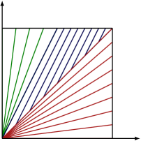
Figure 1: Optimal macroscopic paths that give the last passage time constant described in Theorem 4.1.

We turn to the general hydrodynamic limit. The variational description needs the following ingredients. Define the wedge

$$\mathcal{W}=\{(x,y)\in\mathbb{R}^{2}:y\geq 0,\,x\geq-y\}$$

and on $\mathcal{W}$ the last-passage function of homogeneous TASEP by

$$\gamma(x,y)=(\sqrt{x+y}+\sqrt{y})^{2}.$$ (4.5)

Let $\textbf{x}(s)=(x_{1}(s),x_{2}(s))$ denote a path in $\mathbb{R}^{2}$ and set

$$\mathcal{H}(x,y)=\{\textbf{x}\in C([0,1],\mathcal{W}) :\textbf{x}\text{ is piecewise }C^{1},\textbf{x}(0)=(0,0),$$

$$\textbf{x}(1)=(x,y),\,\textbf{x}^{\prime}(s)\in\mathcal{W}\textrm{ wherever the derivative is defined}\}.$$

The speed function $c$ of our system is by assumption a positive lower semicontinuous function on $\mathbb{R}$. We assume that at each $x\in\mathbb{R}$

$$c(x)=\min\Big{\{}\lim_{y\nearrow x}c(y),\lim_{y\searrow x}c(y)\Big{\}}.$$ (4.6)

In particular we assume that the limits in (4.6) exist. We also assume that $c(x)$ has only finitely many discontinuities in any compact set, hence it is bounded away from $0$ in any compact set.

For the hydrodynamic limit consider a sequence of exclusion processes $\eta^{n}=(\eta^{n}_{i}(t):i\in\mathbb{Z},\,t\in\mathbb{R}_{+})$ indexed by $n\in\mathbb{N}$. These processes are constructed on a common probability space that supports the initial configurations $\{\eta^{n}(0)\}$ and the Poisson clocks of each process. As always, the clocks of process $\eta^{n}$ are independent of its initial state $\eta^{n}(0)$. The joint distributions across the index $n$ are immaterial, except for the assumed initial law of large numbers (4.12) below. In the process $\eta^{n}$ a particle at site $i$ attempts a jump to $i+1$ with rate $c(i/n)$. Thus the generator of $\eta^{n}$ is

$$L_{n}f(\eta)=\sum_{x\in\mathbb{Z}}c(xn^{-1})\eta(x)(1-\eta(x+1))(f(\eta^{x,x+1})-f(\eta))$$ (4.7)

for cylinder functions $f$ on the state space $\{0,1\}^{\mathbb{Z}}$. The usual notation is that particle configurations are denoted by $\eta=(\eta(i):i\in\mathbb{Z})\in\{0,1\}^{\mathbb{Z}}$ and

$$\eta^{x,x+1}(i)=\begin{cases}0&\text{when }i=x\\ 1&\text{when }i=x+1\\ \eta(i)&\text{when }i\neq x,x+1\end{cases}$$

is the configuration that results from moving a particle from $x$ to $x+1$. Let $J_{i}^{n}(t)$ denote the number of particles that have made the jump from site $i$ to site $i+1$ in time interval $[0,t]$ in the process $\eta^{n}.$

An initial macroscopic profile $\rho_{0}$ is a measurable function on $\mathbb{R}$ such that $0\leq\rho_{0}(x)\leq 1$ for all real $x$, with antiderivative $v_{0}$ satisfying

$$v_{0}(0)=0,\quad v_{0}(b)-v_{0}(a)=\int_{a}^{b}\rho_{0}(x)\,dx.$$ (4.8)

The macroscopic flux function of the constant rate 1 TASEP is

$$f(\rho)=\left\{\begin{array}[]{ll}\vspace{0.1 in}\rho(1-\rho),&\textrm{if }0\leq\rho\leq 1\\ -\infty,&\textrm{otherwise. }\end{array}\right.$$ (4.9)

Its Legendre conjugate

$$f^{*}(y)=\inf_{0\leq\rho\leq 1}\{y\rho-f(\rho)\}$$

represents the limit shape in the wedge. We orient our model so that growth in the wedge proceeds upward, and so we use $g(y)=-f^{*}(y)$. It is explicitly given by

$$g(y)=\sup_{0\leq\rho\leq 1}\{f(\rho)-y\rho\}=\left\{\begin{array}[]{lll}\vspace{0.1 in}-y,&\textrm{if }y\leq-1\\ \vspace{0.1 in}\frac{1}{4}{(1-y)^{2}},&\textrm{if }-1\leq y\leq 1\\ 0,&\textrm{if }y\geq 1.\end{array}\right.$$ (4.10)

For $x\in\mathbb{R}$ define $v(x,0)=v_{0}(x)$, and for $t>0,$

$$v(x,t)=\sup_{w(\cdot)}\left\{v_{0}(w(0))-\int_{0}^{t}c(w(s))\,g\left(\dfrac{w^{\prime}(s)}{c(w(s))}\right)\,ds\right\}$$ (4.11)

where the supremum is taken over continuous piecewise $C^{1}$ paths $w:[0,t]\longrightarrow\mathbb{R}$ that satisfy $w(t)=x.$ The function $v(x,t)$ is Lipschitz continuous jointly in $(x,t).$ (see Section 5.2) and it has a derivative almost everywhere. The macroscopic density is defined by $\rho(x,t)=v_{x}(x,t).$

The initial distributions of the processes $\eta^{n}$ are arbitrary subject to the condition that the following strong law of large numbers holds at time $t=0$: for all real $a<b$

$$\lim_{n\rightarrow\infty}\frac{1}{n}\sum_{i=\lfloor{na}\rfloor+1}^{\lfloor{nb}\rfloor}\eta^{n}_{i}(0)=\int_{a}^{b}\rho_{0}(x)\,dx\quad\text{a.s.}$$ (4.12)

The second theorem gives the hydrodynamic limit of current and particle density for TASEP with discontinuous jump rates.

Theorem 4.2.

Let $c(x)$ be a lower semicontinuous positive function satisfying (4.6), with finitely many discontinuities in any compact set. Under assumption (4.12), these strong laws of large numbers hold at each $t>0$: for all real numbers $a<b$

$$\lim_{n\rightarrow\infty}n^{-1}J^{n}_{\lfloor{na}\rfloor}(nt)=v_{0}(a)-v(a,t)\quad a.s.$$ (4.13)

and

$$\lim_{n\rightarrow\infty}\frac{1}{n}\sum_{i=\lfloor{na}\rfloor+1}^{\lfloor{nb}\rfloor}\eta^{n}_{i}(nt)=\int_{a}^{b}\rho(x,t)\,dx\quad a.s.$$ (4.14)

where $v(x,t)$ is defined by (4.11) and $\rho(x,t)=v_{x}(x,t).$

Remark 4.3.

In a totally asymmetric $K$-exclusion with speed function $c$ the state space would be $\{0,1,\dotsc,K\}^{\mathbb{Z}}$ with $K$ particles allowed at each site, and one particle moved from site $x$ to $x+1$ at rate $c(x/n)$ whenever such a move can be legitimately completed. Theorem 4.2 can be proved for this process with the same method of proof. The definition of the limit (4.11) would be the same, except that the explicit flux $f$ and wedge shape $g$ would be replaced by the unknown functions $f$ and $g$ whose existence was proved in [27].

To illustrate Theorem 4.2 we compute the macroscopic density profiles $\rho(x,t)$ from constant initial conditions in the two-phase model with speed function

$$c(x)=c_{1}(1-H(x))+c_{2}H(x)$$ (4.15)

where $H(x)=\mathbf{1}_{[0,\infty)}(x)$ is the Heavyside function and $c_{1}\geq c_{2}$. (The case $c_{1}<c_{2}$ can then be deduced from particle-hole duality.) The particles hit the region of lower speed as they pass the origin from left to right. Depending on the initial density $\rho$, we see the system adjust to this discontinuity in different ways to match the actual throughput of particles on either side of the origin. The maximal flux on the right is $c_{2}/4$ which is realized on the left at densities $\rho^{*}$ and $1-\rho^{*}$ with

$$\rho^{*}=\tfrac{1}{2}-\tfrac{1}{2}\sqrt{1-c_{2}/c_{1}}.$$

Corollary 4.4.

Let $c_{1}\geq c_{2}$ and the speed function as in (4.15). Then the macroscopic density profiles with initial conditions $\rho_{0}(x,0)=\rho$ are given as follows.

(i) Suppose $0<\rho<\rho^{*}$. Define $r^{*}=r^{*}(\rho)=\tfrac{1}{2}-\tfrac{1}{2}\sqrt{1-4\rho(1-\rho)c_{1}/c_{2}}$. Then

$$\rho(x,t)=\left\{\begin{array}[]{llll}\vspace{0.1 in}\rho&\textrm{if }-\infty\leq x\leq 0\\ \vspace{0.1 in}r^{*}&\textrm{if }0\leq x\leq c_{2}(1-2r^{*})t\\ \vspace{0.1 in}\dfrac{1}{2}\left(1-\dfrac{x}{tc_{2}}\right)&\textrm{if }c_{2}(1-2r^{*})t\leq x\leq c_{2}(1-2\rho)t\\ \rho&\textrm{if }(1-2\rho)tc_{2}\leq x<+\infty\end{array}\right.$$ (4.16)

(ii) Suppose $\rho^{*}\leq\rho\leq\frac{1}{2}.$ Then

$$\rho(x,t)=\left\{\begin{array}[]{llll}\vspace{0.1 in}\rho&\textrm{if }-\infty\leq x\leq-tc_{1}(\rho-\rho^{*})\\ \vspace{0.1 in}1-\rho^{*}&\textrm{if }-tc_{1}(\rho-\rho^{*})\leq x\leq 0\\ \vspace{0.1 in}\dfrac{1}{2}\left(1-\dfrac{x}{tc_{2}}\right)&\textrm{if }0\leq x\leq(1-2\rho)tc_{2}\\ \rho&\textrm{if }(1-2\rho)tc_{2}\leq x<+\infty\end{array}\right.$$ (4.17)

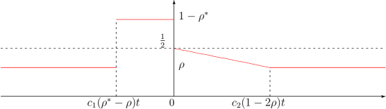
Figure 3: Density profile $\rho(x,t)$ in the two-phase ($c_{1}>c_{2}$) TASEP when we start from constant initial configurations $\rho_{0}(x)\equiv\rho\in[\rho^{*},\tfrac{1}{2}].$

(iii) Suppose $\rho\geq\frac{1}{2}.$ Define $r^{*}=r^{*}(\rho)=\tfrac{1}{2}-\tfrac{1}{2}\sqrt{1-4\rho(1-\rho)c_{2}/c_{1}}$. Then

$$\rho(x,t)=\left\{\begin{array}[]{lll}\vspace{0.1 in}\rho&\textrm{if }-\infty\leq x\leq-tc_{1}(\rho-r^{*})\\ \vspace{0.1 in}1-r^{*}&\textrm{if }-tc_{1}(\rho-r^{*})\leq x\leq 0\\ \rho&\textrm{if }0<x<+\infty\end{array}\right.$$ (4.18)

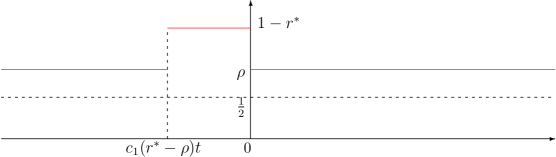
Figure 4: Density profile $\rho(x,t)$ in the two-phase ($c_{1}>c_{2}$) TASEP when we start from constant initial configurations $\rho_{0}(x)\equiv\rho\in(\tfrac{1}{2},1).$

Remark 4.5.

Taking $t\to\infty$ in the three cases of Corollary 4.18 gives a family of macroscopic profiles that are fixed by the time evolution. A natural question to investigate would be the existence and uniqueness of invariant distributions that correspond to these macroscopic profiles.

Next we relate the density profiles picked by the discontinuous TASEP to entropy conditions for scalar conservation laws with discontinuous fluxes. The entropy conditions defined by Adimurthi and Gowda [1] are particularly suited to our needs. Their results give uniqueness of the solution for the scalar conservation law

$$\left\{\begin{array}[]{ll}\vspace{0.1 in}\rho_{t}+\left(F(x,\rho)\right)_{x}=0,&x\in\mathbb{R},t>0\\ \rho(x,0)=\rho_{0}(x),&x\in\mathbb{R}\end{array}\right.$$ (4.19)

with distinct fluxes on the half-lines:

$$F(x,\rho)=H(x)f_{r}(\rho)+(1-H(x))f_{\ell}(\rho)$$ (4.20)

where $f_{r},f_{\ell}\in C^{1}(\mathbb{R})$ are strictly concave with superlinear decay to $-\infty$ as $|x|\to\infty$. A solution of (4.19) means a weak solution, that is, $\rho\in L^{\infty}_{\text{loc}}(\mathbb{R}\times\mathbb{R}_{+})$ such that for all continuously differentiable, compactly supported test functions $\phi\in C_{c}^{1}\left(\mathbb{R}\times\mathbb{R}_{+}\right)$,

$$\int_{-\infty}^{+\infty}\int_{0}^{+\infty}\left(\rho\frac{\partial\phi}{\partial t}+F(x,\rho)\frac{\partial\phi}{\partial x}\right)\,dt\,dx+\int_{-\infty}^{+\infty}\rho(x,0)\phi(x,0)\,dx=0.$$ (4.21)

(4.21) is the weak formulation of the problem

$$\begin{cases}\rho_{t}+f_{r}(\rho)_{x}=0,&\textrm{for }x>0,t>0\\[5.0pt] \rho_{t}+f_{\ell}(\rho)_{x}=0,&\textrm{for }x<0,t>0\\[5.0pt] f_{r}(\rho(0+,t))=f_{\ell}(\rho(0-,t))&\text{for a.e.\ $t>0$}\\[5.0pt] \rho(x,0)=\rho_{0}(x).\end{cases}$$ (4.22)

The entropy conditions used in [1] come in two sets and assume the existence of certain one-sided limits:

$(E_{i})$ Interior entropy condition, or Lax-Oleinik entropy condition:

$$\rho(x+,t)\geq\rho(x-,t)\quad\text{for $x\neq 0$ and for all $t>0$.}$$ (4.23)

$(E_{b})$ Boundary entropy condition at $x=0$: for almost every $t$, the limits $\rho(0\pm,t)$ exist and one of the following holds:

$$f_{r}^{\prime}(\rho(0+,t))\geq 0\quad\textrm{and}\quad f_{\ell}^{\prime}(\rho(0-,t))\geq 0,$$ (4.24)

$$f_{r}^{\prime}(\rho(0+,t))\leq 0\quad\textrm{and}\quad f_{\ell}^{\prime}(\rho(0-,t))\leq 0,$$ (4.25)

$$f_{r}^{\prime}(\rho(0+,t))\leq 0\quad\textrm{and}\quad f_{\ell}^{\prime}(\rho(0-,t))\geq 0.$$ (4.26)

Define

$$G_{x}(p)=\mathbf{1}\{x>0\}f_{r}^{*}(p)+\mathbf{1}\{x<0\}f_{\ell}^{*}(p)+\mathbf{1}\{x=0\}\min\bigl{(}f^{*}_{r}(0),f^{*}_{\ell}(0)\bigr{)},$$

where $f_{r}^{*}$ and $f_{\ell}^{*}$ are the convex duals of $f_{r}$ and $f_{\ell}$. Set $V_{0}(x)=\int_{0}^{x}\rho_{0}(\theta)\,d\theta$ and define

$$V(x,t)=\sup_{w(\cdot)}\left\{V_{0}(w(0))+\int_{0}^{t}G_{w(s)}\bigl{(}w^{\prime}(s)\bigr{)}\,ds\right\}$$ (4.27)

where the supremum is over continuous, piecewise linear paths $w:[0,t]\longrightarrow\mathbb{R}$ with $w(t)=x.$

Theorem 4.6.

[1] Let $\rho_{0}\in L^{\infty}(\mathbb{R})$ and define $V$ by (4.27). Then $V$ is a uniformly Lipschitz continuous function and $\rho(x,t)=V_{x}(x,t)$ is the unique weak solution of (4.22) that satisfies the entropy assumptions $(E_{i})$ and $(E_{b})$ in the class $L^{\infty}\cap BV_{\text{\rm loc}}$ and with discontinuities given by a discrete set of Lipschitz curves.

It is easy to check that the two-phase density profile $\rho(x,t)$ in Corollary 4.18 is a weak solution (in the sense of (4.21)) to the scalar conservation law (4.19) with flux function $F(x,\rho)=c(x)\rho(1-\rho)$. However we cannot immediately apply this theorem in our case since the two-phase flux function $\widetilde{F}(x,\rho)=(1-H(x))c_{1}f(\rho)+H(x)c_{2}f(\rho)$ is finite only for $\rho\in[0,1]$ and in particular is not $C^{1}.$ We show how we can replace $F(x,\rho)$ with $\widetilde{F}(x,\rho)$ in the above theorems in Section 5.4. In particular, we prove the following.

Theorem 4.7.

For $\rho\in\mathbb{R}$ define $f_{r}(\rho)=c_{2}(1-\rho)\rho$ and $f_{\ell}(\rho)=c_{1}(1-\rho)\rho$ to be the flux functions for the scalar conservation law (4.22). Let the initial macroscopic profile for the hydrodynamic limit be a measurable function $0\leq\rho_{0}(x)\leq 1$. Then the macroscopic density profile $\rho(x,t)$ from the hydrodynamic limit in Theorem 4.2 is the unique solution described in Theorem 4.6.

Chapter 5 Multi-phase TASEP

5.1 Wedge last passage time

The strategy of the proof of the hydrodynamic limit is the one from [27] and [28]. Instead of the particle process we work with the height process. The limit is first proved for the jam initial condition of TASEP (also called step initial condition) which for the height process is an initial wedge shape. This process can be equivalently represented by the wedge last-passage model. Subadditivity gives the limit. The general case then follows from an envelope property that also leads to the variational representation of the limiting height profile. In this section we treat the wedge case, and the next section puts it all together.

Recall the notation and conventions introduced in the previous section. In particular, $c(x)$ is a positive, lower semicontinuous speed function with only finitely many discontinuities in any compact set. Define a lattice analogue of the wedge $\mathcal{W}$ by

$$\mathcal{L}=\{(i,j)\in\mathbb{Z}^{2}:j\geq 1,i\geq-j+1\}$$ (5.1)

with boundary $\partial\mathcal{L}=\{(i,0):i\geq 0\}\cup\{(i,-i):i<0\}$.

For each $n\in\mathbb{N}$ construct a last-passage growth model on $\mathcal{L}$ that represents the TASEP height function in the wedge. Let $\{\tau^{n}_{i,j}:(i,j)\in\mathcal{L}\}_{n\in\mathbb{N}}$ denote a sequence of independent collections of i.i.d. exponential rate $1$ random variables. We need an extra index $\ell$ to denote the shifting. Define weights

$$\omega_{i,j}^{n,\ell}=c\left(\dfrac{i-\ell}{n}\right)^{-1},\quad(i,j)\in\mathcal{L}.$$ (5.2)

For $\ell\in\mathbb{Z}$ and $n\in\mathbb{N}$ assign to site $(i,j)\in\mathcal{L}$ the random variable $\omega_{i,j}^{n,\ell}\tau^{n}_{i,j}.$ Given lattice points $(a,b),(u,v)\in\mathcal{L}$, $\Pi((a,b),(u,v))$ is the set of lattice paths $\pi=\{(a,b)=(i_{0},j_{0}),(i_{1},j_{1}),...,(i_{p},j_{p})=(u,v)\}$ whose admissible steps satisfy

$$(i_{l},j_{l})-(i_{l-1},j_{l-1})\in\{(1,0),(0,1),(-1,1)\}.$$ (5.3)

In the case that $(a,b)=(0,1)$ we simply denote this set by $\Pi(u,v)$. For $(u,v)\in\mathcal{L}$, $\ell\in\mathbb{R}$ and $n\in\mathbb{N}$ denote the wedge last passage time

$$T^{n,\ell}(u,v)=\max_{\pi\in\Pi(u,v)}\sum_{(i,j)\in\pi}\omega^{n,\ell}_{i,j}\tau^{n}_{i,j}$$ (5.4)

with boundary conditions

$$T^{n,\ell}(u,v)=0\quad\text{for}\quad(u,v)\in\partial\mathcal{L}.$$ (5.5)

Admissible steps (5.3) come from the properties of the TASEP height function. Notice that $(0,1)$ is in fact never used in a maximizing path.

To describe macroscopic last passage times define, for $(x,y)\in\mathcal{W}$ and $q\in\mathbb{R}$,

$$\Gamma^{q}(x,y)=\sup_{\textbf{x}(\cdot)\in\mathcal{H}(x,y)}\Big{\{}\int_{0}^{1}\frac{\gamma(\textbf{x}^{\prime}(s))}{c(x_{1}(s)-q)}\,ds\Big{\}}.$$ (5.6)

Theorem 5.1.

For all $q\in\mathbb{R}$ and $(x,y)$ in the interior of $\mathcal{W}$

$$\lim_{n\rightarrow\infty}n^{-1}T^{n,\lfloor{nq}\rfloor}(\lfloor{nx}\rfloor,\lfloor{ny}\rfloor)=\Gamma^{q}(x,y)\quad\text{a.s.}$$ (5.7)

Remark 5.2.

In a constant rate $c$ environment the wedge last passage limit is

$$\lim_{n\rightarrow\infty}\frac{1}{n}{T^{n}(\lfloor{nx}\rfloor,\lfloor{ny}\rfloor)}=c^{-1}\gamma(x,y)=c^{-1}\left(\sqrt{x+y}+\sqrt{y}\right)^{2}.$$ (5.8)

The limit $\gamma(x,y)$ is concave, but this is not true in general for $\Gamma^{0}(x,y)$. In some special cases concavity still holds, such as if the function $c(x)$ is nonincreasing if $x<0$ and nondecreasing if $x>0$.

To prove Theorem 5.7 we approximate $c(x)$ with step functions. Let $-\infty=a_{1}<a_{2}<...<a_{L-1}<a_{L}=+\infty,$ and consider the lower semicontinuous step function

$$c(x)=\sum_{m=1}^{L-1}r_{m}\mathbf{1}_{(a_{m},a_{m+1})}(x)+\sum_{m=2}^{L-1}\min\{r_{m-1},r_{m}\}\mathbf{1}_{\{a_{m}\}}(x).$$ (5.9)

Proposition 5.3.

Let $c(x)$ be given by (5.9). Then limit (5.7) holds.

On the way to Proposition 5.3 we state preliminary lemmas that will be used for pieces of paths. We write $c_{i}$ for the rate values instead of $r_{i}$ to be consistent with the notation in Theorem 4.1.

Lemma 5.4.

Assume that there is a unique discontinuity $a_{2}=0$ for the speed function $c(x)$ in (5.9). Then for $y>0$

$$\lim_{n\rightarrow\infty}n^{-1}T^{n,0}(0,\lfloor{ny}\rfloor)=\dfrac{4y}{\min\{c_{1},c_{2}\}}=\int_{0}^{1}\frac{\gamma(0,y)}{c(0)}\,ds\quad\text{a.s.}$$

Proof.

The upper bound in the limit is immediate from domination with constant rates $c(0)$.

For the lower bound we spell out the details for the case $c_{1}\geq c_{2}$. Let $\varepsilon>0$. To bound $T^{n,0}(0,\lfloor{ny}\rfloor)$ from below force the path to go through points $(0,1)$, $\{(\lfloor{ny\varepsilon}\rfloor,(k-1)\lfloor{ny\varepsilon}\rfloor):k=1,\dotsc,\lfloor{\varepsilon^{-1}}\rfloor\}$ and $(0,\lfloor{ny}\rfloor)$. For $1\leq k<\lfloor{\varepsilon^{-1}}\rfloor$ let $T^{n}(R^{n}_{k})$ be the last passage time from $(\lfloor{ny\varepsilon}\rfloor,(k-1)\lfloor{ny\varepsilon}\rfloor)$ to $(\lfloor{ny\varepsilon}\rfloor,k\lfloor{ny\varepsilon}\rfloor)$. $R^{n}_{k}$ refers to the parallelogram that contains all the admissible paths from $(\lfloor{ny\varepsilon}\rfloor,(k-1)\lfloor{ny\varepsilon}\rfloor)$ to $(\lfloor{ny\varepsilon}\rfloor,k\lfloor{ny\varepsilon}\rfloor)$. Each $R^{n}_{k}$ lies to the right of $x=0$ and therefore in the $c_{2}$-rate area. (See Fig. 1.)

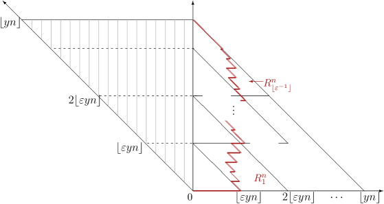
Figure 1: A possible microscopic path forced to go through opposite corners of the parallelograms $R^{n}_{k}$. The striped area left of $x=0$ is the $c_{1}$-rate region.

Let $0<\delta<\varepsilon{c_{2}}^{-1}\gamma(0,y)$. A large deviation estimate (Theorem 4.1 in [26]) gives a constant $C=C(c_{2},y,\varepsilon,\delta)$ such that

$$\mathbb{P}\left\{T^{n}_{c_{2}}(R^{n}_{k})\leq n(\varepsilon{c_{2}}^{-1}\gamma(0,y)-\delta)\right\}\leq e^{-Cn^{2}}.$$ (5.10)

By a Borel-Cantelli argument, for large $n$,

$$T^{n,0}(0,\lfloor{ny}\rfloor) \geq\sum_{k=1}^{\lfloor{\varepsilon^{-1}}\rfloor-1}T^{n}(R^{n}_{k})\geq n(\lfloor{\varepsilon^{-1}}\rfloor-1)(\varepsilon{c_{2}}^{-1}\gamma(0,y)-\delta).$$

This suffices for the conclusion. ∎

Remark 5.5.

This lemma shows why it is convenient to use a lower semi-continuous speed function. A path that starts and ends at the same discontinuity stays mostly in the low rate region to maximize its weight. This translates macroscopically to the formula for the limiting time constant obtained in the lemma, involving only the value of $c$ at the discontinuity. If the speed function is not lower semi-continuous, we can state the same result using left and right limits.

Lemma 5.6.

Let $a=0<b<+\infty$ be discontinuities for the step speed function $c(x)$ and $c(x)=r$ for $a<x<b$. Take $z\in[0,b]$. Let $\widetilde{T}^{n}(\lfloor{nz}\rfloor,\lfloor{ny}\rfloor)$ be the wedge last passage time from $(0,1)$ to $(\lfloor{nz}\rfloor,\lfloor{ny}\rfloor)$ subject to the constraint that the path has to stay in the $r$-rate region $(a,b)\times(0,+\infty)$, except possibly for the initial and final steps. Then

$$\lim_{n\rightarrow\infty}n^{-1}\widetilde{T}^{n}(\lfloor{nz}\rfloor,\lfloor{ny}\rfloor)=r^{-1}{\gamma(z,y)}\quad\text{a.s.}$$ (5.11)

Same statement holds if $b\leq z\leq 0$.

Proof.

The upper bound $\varlimsup n^{-1}\widetilde{T}^{n}(\lfloor{nz}\rfloor,\lfloor{ny}\rfloor)\leq{r}^{-1}{\gamma(z,y)}$ is immediate by putting constant rates $r$ everywhere and dropping the restrictions on the path. For the lower bound adapt the steps of the proof in Lemma 5.4. ∎

Lemma 5.6 is a place where we cannot allow accumulation of discontinuities for the speed function.

Before proceeding to the proof of Proposition 5.3 we make a simple but important observation about the macroscopic paths $\mathbf{x}(s)=(x^{1}(s),x^{2}(s))$, $s\in[0,1]$, in $\mathcal{H}(x,y)$ for the case where $c(x)$ is a step function (5.9).

Lemma 5.7.

There exists a constant $C=C(x,y,c(\cdot-q))$ such that the supremum in (5.6) comes from paths in $\mathcal{H}(x,y)$ that consist of at most $C$ line segments. Apart from the first and last segment, these segments can be of two types: segments that go from one discontinuity of $c(\cdot-q)$ to a neighboring discontinuity, and vertical segments along a discontinuity.

Proof.

Path $\mathbf{x}$ is a union of subpaths $\{\textbf{x}_{j}\}$ along which $c(x_{j}^{1}(s)-q)$ is constant, except possibly at the endpoints. Given such a subpath $(\mathbf{x}_{j}(s):{t_{j}}\leq s\leq{t_{j+1}})$, concavity of $\gamma$ and Jensen’s inequality imply that the line segment $\phi_{j}$ that connects $\textbf{x}_{j}(t_{j})$ to $\textbf{x}_{j}(t_{j+1})$ dominates:

$$\int_{t_{j}}^{t_{j+1}}\frac{\gamma(\textbf{x}_{j}^{\prime}(s))}{c(x_{j}^{1}(s)-q)}\,ds\leq\int_{t_{j}}^{t_{j+1}}\frac{\gamma(\phi_{j}^{\prime}(s))}{c(\phi_{j}^{1}(s)-q)}\,ds.$$

Consequently we can restrict to paths that are unions of line segments.

To bound the number of line segments, observe first that the number of segments that go from one discontinuity to a neighboring discontinuity is bounded. The reason is that the restriction $\textbf{x}^{\prime}(s)\in\mathcal{W}$ forces such a segment to increase at least one of the coordinates by the distance between the discontinuities.

Additionally there can be subpaths that touch the same discontinuity more than once without touching a different discontinuity. Lower semi-continuity of $c(\cdot)$ and Jensen’s inequality show again that the vertical line segment that stays on the discontinuity dominates such a subpath. Consequently there can be at most one (vertical) line segment between two line segments that connect distinct discontinuities. ∎

Next a lemma about the continuity of $\Gamma^{q}$. We write $\Gamma^{q}((a,b),(x,y))$ for the value in (5.6) when the paths go from $(a,b)$ to $(x,y)\in(a,b)+\mathcal{W}$.

Lemma 5.8.

Fix $z,w>0$. Then there exists a constant $C=C(z,w,c(\cdot-q))<\infty$ such that for all $0<\delta\leq 1$ and $0\leq a\leq z$

$$\Gamma^{q}((a,0),(z,\delta))-\Gamma^{q}((a,0),(z,0))\leq C\sqrt{\delta},$$ (5.12)

and for $0\leq b\leq w$

$$\Gamma^{q}((-b,b),(-w,w+\delta))-\Gamma^{q}((-b,b),(-w,w))\leq C\sqrt{\delta}.$$ (5.13)

Proof.

Pick $\delta\in(0,1]$ and consider the point $(z,\delta)$ in $\mathcal{W}$. For any $\mathbf{x}=(x^{1}(s),x^{2}(s))\in\mathcal{H}(z,\delta)$ set

$$I(\textbf{x},q)=\int_{0}^{1}\dfrac{\gamma(\textbf{x}^{\prime}(s))}{c(x^{1}(s)-q)}\,ds.$$ (5.14)

Let $\varepsilon>0$ and assume that $\phi=(\phi^{1},\phi^{2})\in\mathcal{H}(z,\delta)$ is a path such that $\Gamma^{q}(z,\delta)-I(\phi,q)<\varepsilon.$ Lemma 5.7 implies that we can decompose $\phi$ into disjoint linear segments $\phi_{j}$ so that $\phi=\sum_{j=1}^{M}\phi_{j}$ and $\phi_{j}:[s_{j-1},s_{j}]\to\mathcal{W}$. Here $\sum_{j}\phi_{j}$ means path concatenation.

We can find segments $\phi_{j(k)}$, $1\leq k\leq N$, such that

$$\phi^{1}_{j(k)}(s_{j(k)-1})<\phi^{1}_{j(k)}(s_{j(k)}),\quad\phi^{1}_{j(k)}(s_{j(k)})=\phi^{1}_{j(k+1)}(s_{j(k+1)-1}),$$

$\phi^{1}_{j(1)}(s_{j(1)-1})=0$, and $\phi^{1}_{j(N)}(s_{j(N)})=z$. In other words, the projections of the segments $\phi_{j(k)}$ cover the interval $[0,z]$ without overlap and without backtracking.

We bound the contribution of the remaining path segments to $I(\phi,q)$. Let $J$ $=$ $\bigcup_{k=1}^{N-1}[s_{j(k)},s_{j(k+1)-1}]$ be the leftover portion of the time interval $[0,1]$. The subpath $\phi(s)$, $s\in[s_{j(k)},s_{j(k+1)-1}]$, (possibly) eliminated from between $\phi_{j(k)}$ and $\phi_{j(k+1)}$ satisfies $\phi^{1}(s_{j(k)})=\phi^{1}(s_{j(k+1)-1})$. Note that $\gamma(a,b)\leq 2a+4b$ for $(a,b)\in\mathcal{W}$ and $\int_{0}^{1}(\phi^{2})^{\prime}(s)\,ds=\delta$. We can bound as follows:

$$\int_{J}\frac{\gamma((\phi^{1})^{\prime}(s),(\phi^{2})^{\prime}(s))}{c(\phi^{1}(s)-q)}\,ds \leq C\int_{J}\gamma((\phi^{1})^{\prime}(s),(\phi^{2})^{\prime}(s))\,ds$$

$$\leq C\int_{J}\big{(}2(\phi^{1})^{\prime}(s)+4(\phi^{2})^{\prime}(s)\big{)}\,ds$$

$$\leq C\int_{J}2(\phi^{1})^{\prime}(s)\,ds+C\int_{0}^{1}4(\phi^{2})^{\prime}(s)\,ds$$

$$=0+4C\delta.$$ (5.15)

Set $t_{k}=s_{j(k)-1}<u_{k}=s_{j(k)}$. Define a horizontal path $w$ from $(0,0)$ to $(z,0)$ with segments

$$w_{k}(s)=\big{(}\phi_{j(k)}^{1}(s),0\big{)},\quad\text{for }\ t_{k}\leq s\leq u_{k},$$ (5.16)

and constant on the complementary time set $J$.

To get the lemma, we estimate

$$\Gamma^{q}(z ,\delta)-\varepsilon\leq I(\phi,q)=\int_{J}\frac{\gamma(\phi^{\prime}(s))}{c(\phi^{1}(s)-q)}\,ds+\int_{[0,1]\setminus J}\frac{\gamma(\phi^{\prime}(s))}{c(\phi^{1}(s)-q)}\,ds$$

$$\leq C\delta+\sum_{k=1}^{N}\Big{(}I(\phi_{j(k)},q)-I(w_{k},q)\Big{)}+\Gamma^{q}(z,0)$$

$$\leq C\delta+C^{\prime}\sum_{k=1}^{N}\int_{t_{k}}^{u_{k}}\big{(}\gamma(\phi^{\prime}_{j(k)}(s))-\gamma(w^{\prime}_{k}(s))\big{)}\,ds+\Gamma^{q}(z,0)$$

$$\leq C\delta+C^{\prime}\sum_{k=1}^{N}\bigg{(}\int_{t_{k}}^{u_{k}}(\phi^{2})^{\prime}_{j(k)}(s)\,ds+$$

$$\phantom{xxxxxxxxxxxxxxx}+2\int_{t_{k}}^{u_{k}}\sqrt{(\phi^{2})^{\prime}_{j(k)}(s)}\sqrt{(\phi^{1})^{\prime}_{j(k)}(s)+(\phi^{2})^{\prime}_{j(k)}(s)}\,ds\bigg{)}+\Gamma^{q}(z,0)$$

$$\leq C\delta+C^{\prime}\sum_{k=1}^{N}\bigg{(}\int_{t_{k}}^{u_{k}}(\phi^{2})^{\prime}_{j(k)}(s)\,ds\bigg{)}^{\frac{1}{2}}\bigg{(}\int_{t_{k}}^{u_{k}}\big{(}(\phi^{1})^{\prime}_{j(k)}(s)+(\phi^{2})^{\prime}_{j(k)}(s)\big{)}\,ds\bigg{)}^{\frac{1}{2}}+\Gamma^{q}(z,0)$$

$$\leq C\delta+C^{\prime}\bigg{(}\sum_{k=1}^{N}\int_{t_{k}}^{u_{k}}(\phi^{2})^{\prime}_{j(k)}(s)\,ds\bigg{)}^{\frac{1}{2}}\times$$

$$\phantom{xxxxxxxxxxxxx}\times\bigg{(}\sum_{k=1}^{N}\int_{t_{k}}^{u_{k}}\big{(}(\phi^{1})^{\prime}_{j(k)}(s)+(\phi^{2})^{\prime}_{j(k)}(s)\big{)}\,ds\bigg{)}^{\frac{1}{2}}+\Gamma^{q}(z,0)$$

$$\leq C\delta+C^{\prime}\sqrt{\delta}\sum_{k=1}^{N}\int_{t_{k}}^{u_{k}}\big{(}(\phi^{1})^{\prime}_{j(k)}(s)+(\phi^{2})^{\prime}_{j(k)}(s)\big{)}\,ds+\Gamma^{q}(z,0)$$

$$\leq C\delta+C^{\prime}\sqrt{\delta}\sqrt{z+\delta}+\Gamma^{q}(z,0)$$

$$\leq C\delta+C^{\prime}\sqrt{\delta}\sqrt{z}+\Gamma^{q}(z,0).$$

The first inequality (5.12) follows for $a=0$ by letting $\varepsilon$ go to 0. It also follows for all $a\in[0,z]$ by shifting the origin to $a$ which replaces $z$ with $z-a$.

For the second inequality (5.13) the arguments are analogous, so we omit them. ∎

Figure 3: A possible macroscopic path from $(0,0)$ to $(z,\delta)$. The dotted vertical lines are discontinuity columns of $c(\cdot-q).$ The error from eliminating the segments outside the two vertical dashed lines and from eliminating pathologies (like the circled part) is of order $\delta$ and a comparison with the horizontal path leads to an error of order $\sqrt{\delta}$.

Corollary 5.9.

Fix $(x,y)\in\mathcal{W}$. Then there exists $C=C(x,y,c(\cdot-q))<\infty$ such that for all $0<\delta\leq 1$

$$\Gamma^{q}(x,y+\delta)-\Gamma^{q}(x,y)<C\sqrt{\delta}.$$ (5.17)

Proof.

Let $A((a,b),(x,y))$ be the parallelogram with sides parallel to the boundaries of the wedge, north-east corner the point $(x,y)$ and south-west corner at $(a,b)$. If $(a,b)=(0,0)$ we simply write $A(x,y)$.

Let $\varepsilon>0.$ Let $\phi^{\varepsilon}$ a path such that $\Gamma^{q}(x,y+\delta)-I(\phi^{\varepsilon},q)<\varepsilon$. Let $u$ be the point where $\phi^{\varepsilon}$ first intersects the north or the east boundary of $A(x,y)$. Without loss of generality assume it is the north boundary and so $u=(a,y)$ for some $a\in[-y,x]$. Then,

$$\Gamma^{q}(x,y+\delta)-\varepsilon \leq I(\phi^{\varepsilon},q)$$

$$\leq\Gamma^{q}(a,y)+\Gamma^{q}((a,y),(x,y+\delta))$$

$$=\Gamma^{q}(a,y)+\Gamma^{q}((a,y),(x,y))+\Gamma^{q}((a,y),(x,y+\delta))-\Gamma^{q}((a,y),(x,y))$$

$$\leq\Gamma^{q}(x,y)+\Gamma^{q}((a,y),(x,y+\delta))-\Gamma^{q}((a,y),(x,y)).$$ (5.18)

The last inequality gives

$$\Gamma^{q}(x,y+\delta)-\Gamma^{q}(x,y)\leq\Gamma^{q}((a,y),(x,y+\delta))-\Gamma^{q}((a,y),(x,y))+\varepsilon\leq C\sqrt{\delta}+\varepsilon$$ (5.19)

by Lemma 5.13. Let $\varepsilon$ decrease to $0$ to prove the Corollary. ∎

Proof of Proposition 5.3.

Fix $(x,y)$ in the interior of $\mathcal{W}$. For $\mathbf{x}=(x^{1}(s),x^{2}(s))\in\mathcal{H}(x,y)$ set

$$I(\textbf{x},q)=\int_{0}^{1}\dfrac{\gamma(\textbf{x}^{\prime}(s))}{c(x^{1}(s)-q)}\,ds.$$ (5.20)

We prove first

$$\varliminf_{n\rightarrow\infty}n^{-1}T^{n,\lfloor{nq}\rfloor}(\lfloor{nx}\rfloor,\lfloor{ny}\rfloor)\geq\Gamma^{q}(x,y)\equiv\sup_{\textbf{x}(\cdot)\in\mathcal{H}(x,y)}I(\textbf{x},q).$$ (5.21)

It suffices to consider macroscopic paths of the type

$$\textbf{x}(s)=\sum_{j=1}^{H}\textbf{x}_{j}(s)\mathbf{1}_{[s_{j},s_{j+1})}(s)$$ (5.22)

where $H\in\mathbb{N}$, $\textbf{x}_{j}$ is the straight line segment from $\textbf{x}(s_{j})$ to $\textbf{x}(s_{j+1})$, $c(x_{1}(s)-q)=r_{m_{j}}$ is constant for $s\in(s_{j},s_{j+1})$, and by continuity $\textbf{x}_{j}(s_{j+1})=\textbf{x}_{j+1}(s_{j+1})$.

Let $\pi^{n}$ be the microscopic path through points $(0,1)$, $\{\lfloor{n\mathbf{x}_{j}(s_{j})}\rfloor:1\leq j\leq H\}$ and $(\lfloor{nx}\rfloor,\lfloor{ny}\rfloor)$ constructed so that its segments $\pi^{n}_{j}$ satisfy these requirements:

(i) $\pi^{n}_{j}$ lies inside the region where $\omega^{n,\lfloor{nq}\rfloor}_{i,k}=r_{m_{j}}^{-1}$ is constant, except possibly for the initial and final step;

(ii) $\pi^{n}_{j}$ maximizes passage time between its endpoints $\lfloor{n\textbf{x}_{j}(s_{j})}\rfloor$ and $\lfloor{n\textbf{x}_{j+1}(s_{j+1})}\rfloor$ subject to the above requirement.

Let

$$T^{n,\lfloor{nq}\rfloor}_{j}=\max_{\pi^{n}_{j}}\sum_{(i,k)\in\pi^{n}_{j}}\omega^{n,\lfloor{nq}\rfloor}_{i,k}\tau_{i,k}$$ (5.23)

denote the last-passage time of a segment subject to these constraints. Observe that the proofs of Lemmas 5.4 and 5.6 do not depend on the shift parameter $q$, therefore

$$\displaystyle\lim_{n\rightarrow\infty}n^{-1}T^{n,\lfloor{nq}\rfloor}_{j}=\dfrac{\gamma(\textbf{x}_{j}(s_{j})-\textbf{x}_{j+1}(s_{j}))}{r_{m_{j}}}=\int_{s_{j}}^{s_{j+1}}\dfrac{\gamma(\textbf{x}^{\prime}_{j}(s))}{c(x^{1}_{j}(s)-q)}\,ds.$$

Adding up the segments gives the lower bound:

$$\varliminf_{n\rightarrow\infty}n^{-1}T^{n,\lfloor{nq}\rfloor}(\lfloor{nx}\rfloor,\lfloor{ny}\rfloor) \geq\varliminf_{n\rightarrow\infty}\sum_{j}n^{-1}T^{n,\lfloor{nq}\rfloor}_{j}$$

$$=\sum_{j}\int_{s_{j}}^{s_{j+1}}\dfrac{\gamma(\textbf{x}^{\prime}_{j}(s))}{c(x^{1}(s)-q)}\,ds=I(\textbf{x},q).$$

Now for the complementary upper bound

$$\varlimsup_{n\rightarrow\infty}n^{-1}T^{n,\lfloor{nq}\rfloor}(\lfloor{nx}\rfloor,\lfloor{ny}\rfloor)\leq\Gamma^{q}(x,y).$$ (5.24)

Each microscopic path to $(\lfloor{nx}\rfloor,\lfloor{ny}\rfloor)$ is contained in $nA$ for a fixed parallelogram $A\subseteq\mathcal{W}$ with sides parallel to the wedge boundaries. Pick $\varepsilon>0$. Let $r_{*}>0$ be a lower bound on all the rate values that appear in the set $A$. Find $\delta>0$ such that $|\gamma(v)-\gamma(w)|<\varepsilon r_{*}$ for all $v,w\in A$ with $|v-w|<\delta$ and $\delta\leq 1$ so that Corollary 5.17 is valid.

Consider an arbitrary microscopic path from $(0,1)$ to $(\lfloor{nx}\rfloor,\lfloor{ny}\rfloor)$. Given the speed function and $q$, there is a fixed upper bound $Q=Q(x,y)$ on the number of segments of the path that start at one discontinuity column $(\lfloor{na_{i}}\rfloor+\lfloor{nq}\rfloor)\times\mathbb{N}$ and end at a neighboring discontinuity column $(\lfloor{na_{i\pm 1}}\rfloor+\lfloor{nq}\rfloor)\times\mathbb{N}$. The reason is that there is an order $n$ lower bound on the number of lattice steps it takes to travel between distinct discontinuities in $nA$.

Fix $K\in\mathbb{N}$ and partition the interval $[0,y]$ evenly by $b_{j}=jy/K$, $0\leq j\leq K$, so that $y/K<\delta/Q.$ Make the partition finer by adding the $y-$coordinates of the intersection points of discontinuity lines $\{a_{i}+q\}\times\mathbb{R}_{+}$ with the boundary of $A$.

Let $\pi^{n}$ be the maximizing microscopic path. We decompose $\pi^{n}$ into path segments $\{\pi^{n}_{j}:0\leq j<M_{n}\}$ by looking at visits to discontinuity columns $(\lfloor{na_{i}}\rfloor+\lfloor{nq}\rfloor)\times\mathbb{N}$, both repeated visits to the same column and visits to a column different from the previous one. Let $\{0=b_{k_{0}}\leq b_{k_{1}}\leq b_{k_{2}}\leq...\leq b_{k_{M_{n}-1}}\leq b_{k_{M_{n}}}=y\}$ be a sequence of partition points and $\{0=x_{0},\,x_{1}=a_{m_{1}}+q,\,x_{2}=a_{m_{2}}+q,\dotsc,x_{M_{n}}=x\}$ a sequence where $x_{j}$ for $0<j<M_{n}$ are discontinuity points of the shifted speed function $c(\cdot\,-q)$. We can create the path segments and these sequences with the property that segment $\pi^{n}_{j}$ starts at $(\lfloor{nx_{j}}\rfloor,l)$ with $l$ in the range $\lfloor{nb_{k_{j}}}\rfloor\leq l\leq\lfloor{nb_{k_{j}+1}}\rfloor$ and ends at $(\lfloor{nx_{j+1}}\rfloor,l^{\prime})$ with $\lfloor{nb_{k_{j+1}}}\rfloor\leq l^{\prime}\leq\lfloor{nb_{k_{j+1}+1}}\rfloor.$ In an extreme case the entire path $\pi^{n}$ can be a single segment that does not touch discontinuity columns.

In order to have a fixed upper bound on the total number $M_{n}$ of segments, uniformly in $n$, we insist that for $0<j<M_{n}-1$ the labels satisfy:

(i) For odd $j$, $\pi^{n}_{j}$ starts and ends at the same discontinuity column $(\lfloor{nx_{{j}}}\rfloor,\,\cdot\,)$. The rate relevant for segment $\pi^{n}_{j}$ is $r_{\ell_{j}}=c(a_{m_{j}})$.

(ii) For even $j$, $\pi^{n}_{j}$ starts and ends at different neighboring discontinuity columns, and except for the initial and final points, does not touch any discontinuity column and visits only points that are in a region of constant rate $r_{\ell_{j}}$.

The above conditions may create empty segments. This is not harmful. Replace $Q$ with $2Q+2$ to continue having the uniform upper bound $M_{n}\leq Q$.

Let $T(\pi^{n}_{j})$ be the total weight of segment $\pi^{n}_{j}$. Let $\tilde{\pi}^{n}_{j}$ be the maximal path from $(\lfloor{nx_{j}}\rfloor,\lfloor{nb_{k_{j}}}\rfloor)$ to $(\lfloor{nx_{j+1}}\rfloor,\lfloor{nb_{k_{j+1}+1}}\rfloor)$ in an environment with constant weights $\omega_{i,j}=r_{\ell_{j}}^{-1}$ everywhere on the lattice, with total weight $T^{n}_{j}$. $T^{n}_{j}\geq T(\pi^{n}_{j})$, up to an error from the endpoints of $\pi^{n}_{j}$.

Theorem 4.2 in [26] gives a large deviation bound for $T^{n}_{j}$. Consider a constant rate $r$ environment and the maximal weight $T\bigl{(}(\lfloor{nu_{1}}\rfloor,\lfloor{nv_{1}}\rfloor),(\lfloor{nu_{2}}\rfloor,\lfloor{nv_{2}}\rfloor)\bigr{)}$ between two points $(u_{1},v_{1})$ and $(u_{2},v_{2})$ such that their lattice versions can be connected by admissible paths for all $n$. Then there exists a positive constant $C$ such that for $n$ large enough,

$$\mathbb{P}\Bigl{\{}T\bigl{(}(\lfloor{nu_{1}}\rfloor,\lfloor{nv_{1}}\rfloor),(\lfloor{nu_{2}}\rfloor,\lfloor{nv_{2}}\rfloor)\bigr{)}>nr^{-1}\gamma(u_{2}-u_{1},v_{2}-v_{1})+n\varepsilon\Bigr{\}}<e^{-Cn}.$$ (5.25)

There is a fixed finite collection out of which we pick the pairs $\{(x_{j},b_{k_{j}}),(x_{j+1},b_{k_{j+1}+1})\}$ that determine the segments $\tilde{\pi}^{n}_{j}$. By (5.25) and the Borel-Cantelli lemma, a.s. for large enough $n$,

$$T^{n}_{j}\;\leq\;nr_{\ell_{j}}^{-1}\gamma(x_{j+1}-x_{j},b_{k_{j+1}+1}-b_{k_{j}})+n\varepsilon\quad\text{for $0\leq j<M_{n}$.}$$ (5.26)

Define $\delta_{1}>0$ by $y+\delta_{1}=\sum_{j=0}^{M_{n}-1}(b_{k_{j+1}+1}-b_{k_{j}})$. Since $y=\sum_{j=0}^{M_{n}-1}(b_{k_{j+1}}-b_{k_{j}})$ and by the choice of the mesh of the partition $\{b_{k}\}$, we have $\delta_{1}\leq M_{n}\delta/Q\leq\delta$. Think of $(x_{j+1}-x_{j},b_{k_{j+1}+1}-b_{k_{j}})$, $0\leq j<M_{n}$, as the successive segments of a macroscopic path from $(0,0)$ to $(x,y+\delta_{1})$.

For sufficiently large $n$ so that (5.26) is in effect,

$$T^{n,\lfloor{nq}\rfloor}(\lfloor{nx}\rfloor,\lfloor{ny}\rfloor) \leq\sum_{j=1}^{M_{n}}T^{n}_{j}\leq n\sum_{j=1}^{M_{n}}r_{\ell_{j}}^{-1}\gamma(x_{j+1}-x_{j},b_{k_{j+1}+1}-b_{k_{j}})+nQ\varepsilon$$

$$\leq n\Gamma^{q}(x,y+\delta_{1})+nQ\varepsilon$$

$$\leq n\Gamma^{q}(x,y)+nC\sqrt{\delta}+nQ\varepsilon.$$

The last inequality came from Corollary 5.17. Let $\delta\rightarrow 0$. Since $\varepsilon$ was arbitrary the upper bound (5.24) holds. ∎

Proof of Theorem 5.7.

Fix $(x,y)$. For each $\varepsilon>0$ we can find lower semicontinuous step functions $c_{1}$ and $c_{2}$ such that $\|c_{1}-c_{2}\|_{\infty}\leq\varepsilon$ and on some compact interval, large enough to contain all the rates that can potentially influence $\Gamma^{q}(x,y)$, $c_{1}(x)\leq c(x)\leq c_{2}(x)$. When the weights in (5.2) come from speed function $c_{i}$ let us write $T_{i}$ for last passage times and $\Gamma_{i}$ for their limits. An obvious coupling using common exponential variables $\{\tau_{i,j}\}$ gives

$$T_{1}^{n,\lfloor{nq}\rfloor}(\lfloor{nx}\rfloor,\lfloor{ny}\rfloor)\geq T^{n,\lfloor{nq}\rfloor}(\lfloor{nx}\rfloor,\lfloor{ny}\rfloor)\geq T^{n,\lfloor{nq}\rfloor}_{2}(\lfloor{nx}\rfloor,\lfloor{ny}\rfloor).$$

Letting $\alpha>0$ denote a lower bound for $c(x)$ in the compact interval relevant for $(x,y)$, we have this bound for $\textbf{x}\in\mathcal{H}(x,y)$:

$$0\leq\int_{0}^{1}\Bigl{\{}\frac{\gamma(\textbf{x}^{\prime}(s))}{c_{1}(x_{1}(s)-q)}-\frac{\gamma(\textbf{x}^{\prime}(s))}{c_{2}(x_{1}(s)-q)}\Bigr{\}}\,ds \leq\varepsilon\int_{0}^{1}\frac{\gamma(\textbf{x}^{\prime}(s))}{c^{2}_{1}(x_{1}(s)-q)}\,ds$$

$$\leq\varepsilon\alpha^{-2}\gamma(x,y).$$

Therefore the limits also have the bound

$$0\leq\Gamma^{q}_{1}(x,y)-\Gamma^{q}_{2}(x,y)\leq C(x,y)\varepsilon.$$

From these approximations and the limits for $T_{i}$ in Proposition 5.3 we can deduce Theorem 5.7. ∎

Proof of Theorem 4.1.

We can construct the last passage times $G(x,y)$ of the corner growth model (4.4) with the same ingredients as the wedge last passage times $T^{n,0}(x,y)$ of (5.4), by taking $Y_{(i,j)}=\omega^{n,0}_{i-j,\,j}\tau^{n}_{i-j,\,j}$. Then $T^{n,0}(x,y)=G(x+y,y)$ and we can transfer the problem to the wedge. The correct speed function to use is now $c(x)=c_{1}\mathbf{1}\{x<0\}+c_{2}\mathbf{1}\{x\geq 0\}$. In this case the limit in Theorem 5.7 can be solved explicitly with calculus. We omit the details. ∎

5.2 Hydrodynamic limit

In this section we sketch the proof of the main result Theorem 4.2. This argument is from [27, 28].

5.2.1 Construction of the process and the variational coupling

For each $n\in\mathbb{N}$ we construct a $\mathbb{Z}$-valued height process $z^{n}(t)=(z^{n}_{i}(t):i\in\mathbb{Z})$. The height values obey the constraint

$$0\leq z^{n}_{i+1}(t)-z^{n}_{i}(t)\leq 1.$$ (5.27)

Let $\{\mathcal{D}^{n}_{i}\}$ be a collection of mutually independent (in $i$ and $n$) Poisson processes with rates $c_{i}^{n}$ given by

$$c_{i}^{n}=c(n^{-1}i),$$ (5.28)

where $c(x)$ is the lower semicontinuous speed function. Dynamically, for each $n$ and $i$, the height value $z^{n}_{i}$ is decreased by $1$ at event times of $\mathcal{D}^{n}_{i}$, provided the new configuration does not violate (5.27).

After we construct $z^{n}(t)$, we can define the exclusion process $\eta^{n}(t)$ by

$$\eta^{n}_{i}(t)=z^{n}_{i}(t)-z^{n}_{i-1}(t).$$ (5.29)

A decrease in $z^{n}_{i}$ is associated with an exclusion particle jump from site $i$ to $i+1$. Thus the $z^{n}$ process keeps track of the current of the $\eta^{n}$-process, precisely speaking

$$J^{n}_{i}(t)=z^{n}_{i}(0)-z^{n}_{i}(t).$$ (5.30)

Assume that the processes $z^{n}$ have been constructed on a probability space that supports the initial configurations $z^{n}(0)=(z^{n}_{i}(0))$ and the Poisson processes $\{\mathcal{D}^{n}_{i}\}$ that are independent of $(z^{n}_{i}(0))$. Next we state the envelope property that is the key tool for the proof of the hydrodynamic limit. Define a family of auxiliary height processes $\{\xi^{n,k}:n\in\mathbb{N},\,k\in\mathbb{Z}\}$ that grow upward from wedge-shaped initial conditions

$$\xi_{i}^{n,k}(0)=\left\{\begin{array}[]{ll}\vspace{0.1 in}0,&\textrm{if }i\geq 0\\ -i,&\textrm{if }i<0.\end{array}\right.$$ (5.31)

The dynamical rule for the $\xi^{n,k}$ process is that $\xi^{n,k}_{i}$ jumps up by 1 at the event times of $\mathcal{D}^{n}_{i+k}$ provided the inequalities

$$\xi^{n,k}_{i}\leq\xi^{n,k}_{i-1}\quad\text{and}\quad\xi^{n,k}_{i}\leq\xi^{n,k}_{i+1}+1$$ (5.32)

are not violated. In particular $\xi^{n,k}_{i}$ attempts a jump at rate $c^{n}_{i+k}$.

Lemma 5.10 (Envelope Property).

For each $n\in\mathbb{N}$, for all $i\in\mathbb{Z}$ and $t\geq 0$,

$$z^{n}_{i}(t)=\sup_{k\in\mathbb{Z}}\{z^{n}_{k}(0)-\xi^{n,k}_{i-k}(t)\}\quad a.s.$$ (5.33)

Equation (5.33) holds by construction at time $t=0$, and it is proved by induction on jumps. For details see Lemma 4.2 in [27].

5.2.2 The limit for $\xi$

For $q,x\in\mathbb{R}$, $t>0$ and for the speed function $c(x)$, define

$$g^{q}(x,t)=\inf\left\{y:(x,y)\in\mathcal{W},\Gamma^{q}(x,y)\geq t\right\}.$$ (5.34)

$\Gamma^{q}(x,y)$ defined by (5.6) represents the macroscopic time it takes a $\xi$-type interface process to reach point $(x,y).$ The level curve of $\Gamma^{q}$ given by $g^{q}(\cdot,t)$ represents the limiting interface of a certain $\xi$-process, as stated in the next proposition.

Proposition 5.11.

For all $q,x\in\mathbb{R}$ and $t>0$

$$\lim_{n\rightarrow\infty}n^{-1}\xi^{n,\lfloor{nq}\rfloor}_{\lfloor{nx}\rfloor}(nt)=g^{-q}(x,t)\quad a.s.$$ (5.35)

Recall the lattice wedge $\mathcal{L}$ defined by (5.1). For $(i,j)\in\mathcal{L}\cup\partial\mathcal{L}$, let

$$L^{n,k}(i,j)=\inf\{t\geq 0:\xi^{n,k}_{i}(t)\geq j\}$$ (5.36)

denote the time when $\xi^{n,k}_{i}$ reaches level $j$. The rules (5.31)–(5.32) give the boundary conditions

$$L^{n,k}(i,j)=0\quad\text{for}\quad(i,j)\in\partial\mathcal{L}$$ (5.37)

and for $(i,j)\in\mathcal{L}$ the recurrence

$$L^{n,k}(i,j)=\max\{L^{n,k}(i-1,j),L^{n,k}(i,j-1),L^{n,k}(i+1,j-1)\}+\beta^{n,k}_{i,j}$$ (5.38)

where $\beta^{n,k}_{i,j}$ is an exponential waiting time, independent of everything else. It represents the time $\xi^{n,k}_{i}$ waits to jump, after $\xi^{n,k}_{i}$ and its neighbors $\xi^{n,k}_{i-1}$, $\xi^{n,k}_{i+1}$ have reached positions that permit $\xi^{n,k}_{i}$ to jump from $j-1$ to $j$. The dynamical rule that governs the jumps of $\xi^{n,k}_{i}$ implies that $\beta^{n,k}_{i,j}$ has rate $c^{n}_{i+k}$.

Equations (5.4), (5.5), (5.37), and (5.38), together with the strong Markov property, imply that

$$\{L^{n,k}(i,j):(i,j)\in\mathcal{L}\cup\partial\mathcal{L}\}\,\overset{\mathcal{D}}{=}\,\{T^{n,-k}(i,j):(i,j)\in\mathcal{L}\cup\partial\mathcal{L}\}.$$ (5.39)

Consequently Theorem 5.7 gives the a.s. convergence $n^{-1}L^{n,\lfloor{nq}\rfloor}(\lfloor{nx}\rfloor,\lfloor{ny}\rfloor)\to\Gamma^{-q}(x,y)$, and this passage time limit gives limit (5.35).

Proof of Theorem 4.2.

Given the initial configurations $\eta^{n}(0)=\left\{\eta^{n}_{i}(0):i\in\mathbb{Z}\right\}$ that appear in hypothesis (4.12), define initial configurations $z^{n}(0)=\left\{z^{n}_{i}(0):i\in\mathbb{Z}\right\}$ so that $z^{n}_{0}(0)=0$ so that (5.29) holds at time $t=0.$ Hypothesis (4.12) implies that

$$\lim_{n\rightarrow\infty}n^{-1}z^{n}_{\lfloor{nq}\rfloor}=v_{0}(q)\quad\textrm{a.s.}$$ (5.40)

for all $q\in\mathbb{R}$, with $v_{0}$ defined by (4.8).

Construct the height processes $z^{n}$ and define the exclusion processes $\eta^{n}$ by (5.29). Define $v(x,t)$ by (4.11). From (5.29)–(5.30) we see that Theorem 4.2 follows from proving that for all $x\in\mathbb{R},t\in\mathbb{R}^{+},$

$$\lim_{n\rightarrow\infty}n^{-1}z^{n}_{\lfloor{nx}\rfloor}(nt)=v(x,t)\quad\textrm{a.s.}$$ (5.41)

Rewrite (5.33) with the correct scaling:

$$n^{-1}z^{n}_{\lfloor{nx}\rfloor}(nt)=\sup_{q\in\mathbb{R}}\left\{n^{-1}z^{n}_{\lfloor{nq}\rfloor}(0)-n^{-1}\xi^{\lfloor{nq}\rfloor}_{\lfloor{nx}\rfloor-\lfloor{nq}\rfloor}(nt)\right\}.$$ (5.42)

The proof of (5.41) is now to show that the right-hand side of (5.42) converges to the right-hand side of (4.11).

From (5.40), (5.42) and (5.35) we can prove that a.s.

$$\lim_{n\rightarrow\infty}n^{-1}z^{n}_{\lfloor{nx}\rfloor}(nt)=\sup_{q\in\mathbb{R}}\left\{v_{0}(q)-g^{-q}(x-q,t)\right\}\equiv\tilde{v}(x,t).$$ (5.43)

The argument is the same as the one from equations (6.4)–(6.15) in [27] so we will not repeat it here.

Using (5.6) and (5.34) we can rewrite $\tilde{v}(x,t)$ as

$$\tilde{v}(x,t)=\sup_{q,y\in\mathbb{R}}\Big{\{}v_{0}(q)-y:\exists\textbf{x}\in\mathcal{H}(x-q,y)\textrm{ such that }\int_{0}^{1}\frac{\gamma(\textbf{x}^{\prime}(s))}{c(x_{1}(s)+q)}\,ds\geq t\Big{\}}.$$ (5.44)

The final step is to prove $v(x,t)=\tilde{v}(x,t).$ The argument is identical to the one used to prove Proposition 4.3 in [28] so we omit it. With this we can consider Theorem 4.2 proved. ∎

5.3 Density profiles in two-phase TASEP

This section proves Corollary 4.18: assuming $c(x)=(1-H(x))c_{1}+H(x)c_{2}$, $c_{1}\geq c_{2}$ and $\rho_{0}(x)\equiv\rho\in(0,1)$, we use variational formula (4.11) to obtain explicit hydrodynamic limits.

Remark 5.12.

In light of Theorem 4.7, one can (instead of doing the following computations) guess the candidate solution for the scalar conservation law (4.22) and then check that it verifies the entropy conditions (4.24) - (4.26). The following computations do not require any knowledge of p.d.e. theory or familiarity with interface problems so we present them independently in this section.

Let

$$C^{0}(x,t,q)=\left\{w\in C([0,t],\mathbb{R}):w\text{ piecewise linear, }w(0)=q,w(t)=x\right\}.$$ (5.45)

To optimize in (4.11) we use a couple different approaches for different cases. We outline this and omit the details.

One approach is to separate the choice of the starting point $q$ of the path. By setting

$$I(x,t,q)=\inf_{w\in C^{0}(x,t,q)}\bigg{\{}\int_{0}^{t}c(w(s))g\left(\dfrac{w^{\prime}(s)}{c(w(s))}\right)\,ds\bigg{\}}$$ (5.46)

(4.11) becomes

$$v(x,t)=\sup_{q\in\mathbb{R}}\left\{v_{0}(q)-I(x,t,q)\right\}.$$ (5.47)

We distinguish four cases according to the signs of $x,q$. Set

$$R_{+}(x,t)=\sup_{q>0}\left\{v_{0}(q)-I(x,t,q)\right\},\textrm{ if }x>0,\quad$$ (5.48)

$$L_{-}(x,t)=\sup_{q<0}\left\{v_{0}(q)-I(x,t,q)\right\},\textrm{ if }x<0.$$ (5.49)

These functions are going to be used in Cases 1 and 2 below ($qx\geq 0$) where we can compute $I(x,t,q)$ directly.

However, there are values $(x,t,q)$ for which the $q$-derivative of the expression in braces in (5.47) is a rational function with a quartic polynomial in the numerator. While an explicit formula for roots of a quartic exists, the solution is not attractive and it is not clear how to pick the right root. Instead we turn the problem into a two-dimensional maximization problem.

If $qx<0$ the optimizing path $w$ crosses the origin: $w(u)=0$ for some $u$. It turns out convenient to find the optimal $q$ for each crossing time $u$. For Case 3 ($q<0,x>0$) set

$$\Phi(u,q)=q\rho-c_{1}ug\left(\dfrac{-q}{uc_{1}}\right)-c_{2}(t-u)g\left(\dfrac{x}{(t-u)c_{2}}\right)$$ (5.50)

and

$$L_{+}(x,t)=\displaystyle\sup_{q<0,u\in[0,t]}\Phi(u,q).$$ (5.51)

For Case 4 ($q>0,x<0$) the obvious modifications are

$$\Psi(u,q)=q\rho-c_{2}ug\left(\dfrac{-q}{uc_{2}}\right)-c_{1}(t-u)g\left(\dfrac{x}{(t-u)c_{1}}\right)$$ (5.52)

and

$$R_{-}(x,t)=\displaystyle\sup_{q>0,u\in[0,t]}\Psi(u,q).$$

Rewrite (5.47) using functions $R_{\pm}$, $L_{\pm}$:

$$v(x,t)=\max\{R_{+}(x,t),L_{+}(x,t)\}\mathbf{1}\{x\geq 0\}+\max\{R_{-}(x,t),L_{-}(x,t)\}\mathbf{1}\{x<0\}.$$ (5.53)

Proof of Corollary 4.18
.

We compute the functions $R_{\pm}$, $L_{\pm}$. The density profiles $\rho(x,t)$ are given then by the $x$-derivative of $v(x,t)$.

Case 1: $x\geq 0$, $q\geq 0$. Since $c_{2}\leq c_{1}$, the minimizing $w$ of $I(x,t,q)$ is the straight line connecting $(0,q)$ to $(t,x).$ In particular,

$$I(x,t,q)=c_{2}tg\left(\frac{x-q}{tc_{2}}\right).$$ (5.54)

Then the resulting $R_{+}(x,t)$ is given by

$$R_{+}(x,t)=\begin{cases}-tc_{2}g(\frac{x}{tc_{2}})&\textrm{if }\rho\leq\frac{1}{2},\quad x<tc_{2}(1-2\rho)\\[4.0pt] \rho x-tc_{2}\rho(1-\rho),&\textrm{if }\rho\leq\frac{1}{2},\quad x\geq tc_{2}(1-2\rho)\\[4.0pt] \rho x-tc_{2}\rho(1-\rho),&\textrm{if }\rho>\frac{1}{2},\end{cases}$$ (5.55)

Case 2: $x\leq 0$, $q\leq 0$. The minimizing path $w$ can either be a straight line from $(0,q)$ to $(t,x)$ or a piecewise linear path such that the set $\{t:w(t)=0\}$ has positive Lebesgue measure. This last statement just says that the path might want to take advantage of the low rate at $x=0$. We leave the calculus details to the reader and record the resulting minimum value of $I(x,t,q)$. Set $B=\sqrt{c_{1}(c_{1}-c_{2})}$.

$$I(x,t,q)=\begin{cases}\vspace{0.07in}\frac{-qc_{1}}{4B}\left(1-\frac{B}{c_{1}}\right)^{2}+\left(t-\frac{|x|-q}{B}\right)\frac{c_{2}}{4}-\frac{xc_{1}}{4B}\left(1+\frac{B}{c_{1}}\right)^{2},\\ \quad\quad\quad\quad\quad\quad\quad\quad\text{when }-(\sqrt{Bt}-\sqrt{|x|})^{2}\leq q,\,-Bt\leq x<0\quad\\ c_{1}tg\left(\frac{x-q}{c_{1}t}\right)\quad\quad\quad\text{otherwise }\end{cases}$$ (5.56)

The corresponding function $L_{-}(x,t)$ is given by

$$L_{-}(x,t)=\begin{cases}\vspace{0.07 in}\rho x-tc_{1}\rho(1-\rho),&0<\rho<\rho^{*},x\in\mathbb{R}\\ \vspace{0.07 in}\rho x-tc_{1}\rho(1-\rho),&\rho^{*}\leq\rho\leq\frac{1}{2},\quad x\leq-tc_{1}(\rho-\rho^{*})\\ \vspace{0.07 in}-\left(t+\frac{x}{B}\right)\frac{c_{2}}{4}+\frac{xc_{1}}{4B}\left(1+\frac{B}{c_{1}}\right)^{2},&\rho^{*}\leq\rho\leq\frac{1}{2},\quad x>-tc_{1}(\rho-\rho^{*})\\ \vspace{0.07 in}\rho x-tc_{1}\rho(1-\rho),&\frac{1}{2}<\rho\leq 1-\rho^{*},\quad x<-tc_{1}(\rho-\rho^{*})\\ \vspace{0.07 in}-\left(t+\frac{x}{B}\right)\frac{c_{2}}{4}+\frac{xc_{1}}{4B}\left(1+\frac{B}{c_{1}}\right)^{2},&\frac{1}{2}<\rho\leq 1-\rho^{*},\quad-tc_{1}(\rho-\rho^{*})\leq x\\ \vspace{0.07 in}-\left(t+\frac{x}{B}\right)\frac{c_{2}}{4}+\frac{xc_{1}}{4B}\left(1+\frac{B}{c_{1}}\right)^{2},&1-\rho^{*}<\rho<1,\quad-Bt\leq x\\ \vspace{0.07 in}-tc_{1}g\big{(}\frac{x}{tc_{1}}\big{)},&1-\rho^{*}<\rho<1,\quad-c_{1}t(2\rho-1)\leq x<-Bt\\ \vspace{0.07 in}\rho x-c_{1}t\rho(1-\rho),&1-\rho^{*}<\rho<1,\quad x<-c_{1}t(2\rho-1)\\ \end{cases}$$ (5.57)

Case 3: $x>0$, $q\leq 0.$ Abbreviate $D=c_{2}^{2}-4c_{1}c_{2}\rho(1-\rho)$. First compute the $q$-derivative

$$\Phi_{q}(u,q)=\begin{cases}\vspace{0.07 in}\rho-\frac{1}{2}-\frac{q}{2uc_{1}},&-uc_{1}\leq q<0\\ \rho&q<-uc_{1}.\end{cases}$$ (5.58)

If $\rho\geq 1/2$ then $\Phi_{q}$ is positive and the maximum value is when $q=0$ so we are reduced to Case $1$. If $\rho<1/2$ the maximizing $\displaystyle q=uc_{1}\left(2\rho-1\right).$ Then

$$F(u)=\Phi\bigl{(}u,2uc_{1}(\rho-\tfrac{1}{2})\bigr{)}=-uc_{1}\rho(1-\rho)-c_{2}(t-u)g\left(\dfrac{x}{(t-u)c_{2}}\right),$$

with $u$-derivative

$$\frac{dF}{du}=-c_{1}\rho(1-\rho)+\frac{c_{2}}{4}\left(1-\frac{x^{2}}{(c_{2}(t-u))^{2}}\right).$$

Again we need to split two cases. If $\rho<\rho^{*}$ (equivalently $D>0$) and $x\leq t\sqrt{D}$, the maximizing $u=t-x/\sqrt{D},$ otherwise $u=0$. If $\rho^{*}\leq\rho<\frac{1}{2}$ the derivative is negative so the maximizing $u$ is still $u=0.$ Together,

$$L_{+}(x,t)=\begin{cases}\vspace{0.07 in}-tc_{1}\rho(1-\rho)+x\Big{(}\frac{1}{2}-\frac{\sqrt{D}}{2c_{2}}\Big{)},&\rho<\rho^{*},x\leq t\sqrt{D}\\ \vspace{0.07 in}-c_{2}tg\big{(}\frac{x}{tc_{2}}\big{)},&\rho<\rho^{*},x\geq t\sqrt{D}\\ -c_{2}tg\big{(}\frac{x}{tc_{2}}\big{)},&\rho^{*}\leq\rho\leq 1.\par\end{cases}$$ (5.59)

Case 4: $x\leq 0,q\geq 0.$ We treat this case in exactly the same way as Case 3, so we omit the details. Here we need the quantity $D_{1}=(c_{1})^{2}-4c_{1}c_{2}\rho(1-\rho)$ and we compute

$$R_{-}(x,t)=\begin{cases}\vspace{0.07 in}-tc_{1}g\big{(}\frac{x}{tc_{1}}\big{)},&\rho\leq\frac{1}{2}\\ \vspace{0.07 in}-tc_{2}\rho(1-\rho)+x\Big{(}\frac{1}{2}+\frac{\sqrt{D_{1}}}{2c_{1}}\Big{)},&\frac{1}{2}<\rho,-t\sqrt{D_{1}}\leq x\\ -tc_{1}g\big{(}\frac{x}{tc_{1}}\big{)},&\frac{1}{2}\leq\rho\leq 1,x<-t\sqrt{D_{1}}\\ \end{cases}$$ (5.60)

Now compute $v(x,t)$ from (5.53). We leave the remaining details to the reader. ∎

5.4 Entropy solutions of the discontinuous conservation law

For this section, $c(x)=(1-H(x))c_{1}+H(x)c_{2}$, $h(\rho)=\rho(1-\rho)$ and set $F(x,\rho)=c(x)h(\rho)$ for the flux function of the scalar conservation law (4.19) and $\widetilde{F}(x,\rho)=c(x)f(\rho)$ for the flux function of the particle system, where $f$ is given by (4.9). (The difference between $F$ and $\widetilde{F}$ is that the latter is $-\infty$ outside $0\leq\rho\leq 1$.)

In [1] the authors prove that there exists a solution to the corresponding Hamilton-Jacobi equation

$$\left\{\begin{array}[]{lll}\vspace{0.1 in}V_{t}+c_{1}h(V_{x})=0,&\textrm{if }x<0,t>0\\ \vspace{0.1 in}V_{t}+c_{2}h(V_{x})=0,&\textrm{if }x>0,t>0\\ V(x,0)=V_{0}(x)\end{array}\right.$$ (5.61)

such that $V_{x}$ solves the scalar conservation law (4.19) with flux function $F(x,\rho)$ and $V_{x}$ satisfies the entropy assumptions $(E_{i}),(E_{b})$. $V(x,t)$ is given by

$$V(x,t)=\sup_{w(\cdot)}\left\{V_{0}(w(0))+\int_{0}^{t}(c(w(s))h)^{*}(w^{\prime}(s))\,ds\right\},$$ (5.62)

where the supremum is taken over piecewise linear paths $w\in C([0,t],\mathbb{R})$ that satisfy $w(t)=x.$

To apply the results of [1] to the profile $\rho(x,t)$ coming from our hydrodynamic limit, we only need to show that the variational descriptions match, in other words that we can replace $F$ with $\widetilde{F}$ and the solution is still the same.

Proof of Theorem 4.7.

Convex duality gives $\left(c(x)f\right)^{*}(y)=c(x)f^{*}\left(y/c(x)\right)$ and so we can rewrite (4.11) as

$$v(x,t)=\sup_{w(\cdot)}\left\{v_{0}(w(0))+\int_{0}^{t}(c(w(s))f)^{*}(w^{\prime}(s))\,ds\right\}.$$ (5.63)

Observe that for all $y\in\mathbb{R}$

$$(c(x)f)^{*}(y)\geq(c(x)h)^{*}(y),$$ (5.64)

with equality if and only if $y\in[-c_{1},c_{2}]$ Since the supremum in (5.62) and (5.63) is taken over the same set of paths, (5.64) implies that

$$V(x,t)\leq v(x,t).$$ (5.65)

The proof of the theorem is now reduced to proving that the supremum in (5.63) is achieved when $w^{\prime}(s)c(w(s))^{-1}\in[-1,1],$ giving $V(x,t)=v(x,t)$.

To this end we rewrite $v(x,t)$ once more, this time as

$$v(x,t)=\max\{R_{+}(x,t),L_{+}(x,t)\}\mathbf{1}\{x\geq 0\}+\max\{R_{-}(x,t),L_{-}(x,t)\}\mathbf{1}\{x<0\}$$

where the functions $R_{\pm}$, $L_{\pm}$ (as in the proof of Corollary 4.18) are defined by

$$R_{+}(x,t)=\sup_{q>0}\left\{v_{0}(q)-I(x,t,q)\right\},\textrm{ if }x>0,\quad$$ (5.66)

$$L_{-}(x,t)=\sup_{q<0}\left\{v_{0}(q)-I(x,t,q)\right\},\textrm{ if }x<0,$$ (5.67)

where $I(x,t,q)$ is as in (5.46), and

$$L_{+}(x,t)=\displaystyle\sup_{q<0,u\in[0,t]}\bigg{\{}v_{0}(q)-c_{1}ug\Big{(}\frac{-q}{uc_{1}}\Big{)}-c_{2}(t-u)g\Big{(}\frac{x}{(t-u)c_{2}}\Big{)}\bigg{\}}\quad\textrm{if }x\geq 0,$$ (5.68)

and

$$R_{-}(x,t)=\displaystyle\sup_{q>0,u\in[0,t]}\bigg{\{}v_{0}(q)-c_{2}ug\left(\dfrac{-q}{uc_{2}}\right)-c_{1}(t-u)g\left(\dfrac{x}{(t-u)c_{1}}\right)\bigg{\}},\quad x\leq 0.$$ (5.69)

It suffices to show that the suprema that define $R_{\pm}$, $L_{\pm}$ are achieved when

$$w^{\prime}(s)c(w(s))^{-1}\in[-1,1].$$ (5.70)

We show this for $L_{+}$. The remaining cases are similar. In (5.68), as before, $u$ is the time for which $w(u)=0.$ Let $\Phi(u,q)$ denote the expression in braces in (5.68) with $q$-derivative

$$\Phi_{q}(u,q)=\begin{cases}\vspace{0.07 in}\rho_{0}(q)-\frac{1}{2}-\frac{q}{2uc_{1}},&-uc_{1}\leq q<0\\ \rho_{0}(q),&q<-uc_{1}.\end{cases}$$ (5.71)

Observe that if $\Phi_{q}(u,q)=0$ for some $q^{*}=q^{*}(u)$ then also $q^{*}$ maximizes $\Phi$. Otherwise the maximum is achieved at $0$ and we are reduced to a different case. Assume that $q^{*}$ exists. Then by (5.71)

$$\frac{-q^{*}}{u}=(1-2\rho_{0}(q^{*}))c_{1}<c_{1}.$$ (5.72)

Therefore, the slope of the first segment of the maximizing path $w$ satisfies (5.70).

The slope of the second segment is $x(t-u)^{-1}.$ Assume that the piecewise linear path $w$ defined by $u$ and $q^{*}$ is the one that achieves the supremum. Also assume $u>t-xc_{2}^{-1}.$ Consider the path $\tilde{w}$ with $\tilde{w}(0)=q^{*}$ and $\tilde{w}(t-xc_{2}^{-1})=0$. Since $g$ is decreasing, we only increase the value of $\Phi$. Hence the supremum that gives $L_{+}$ cannot be achieved on $w$ and this gives the desired contradiction. ∎

Appendix A Basic Facts

In this section we report all basics facts from analysis, special functions and probability theory used throughout the thesis.

A.1 Special functions and distributions

The gamma function is

$$\Gamma(s)=\int_{0}^{\infty}x^{s-1}e^{-x}\,dx.$$

We only use it for positive real values of $s$.

The logarithm $\log\Gamma(s)$ is convex and infinitely differentiable on $(0,\infty)$. The derivatives are called polygamma functions $\Psi_{n}(s)=(d^{n+1}/ds^{n+1})\log\Gamma(s)$, defined for $n\in\mathbb{Z}_{+}$. For $n\geq 1$, $\Psi_{n}$ is nonzero and has sign $(-1)^{n-1}$ throughout $(0,\infty)$. In particular, $\Psi_{0}(s)$ is strictly increasing and has a vertical asymptote at $s=0$. It can be given by

$$\Psi_{0}(1+x)=-\gamma+\sum_{k=1}^{\infty}\frac{x}{k(x+k)}.$$ (A.1)

One way to compute the limit (3.19) is by multiple uses of L’ Hospital’s rule and then an asymptotic analysis for $\Psi_{1}(s)$ for $s\rightarrow 0$. For the asymptotic analysis, we need

$$\Psi_{1}(s)=\sum_{k=0}^{\infty}\frac{1}{(k+s)^{2}}.$$

The Gamma$(\theta,1)$ distribution has density

$$\Gamma(\theta)^{-1}x^{\theta-1}e^{-x},\quad\theta>0.$$ (A.2)

on $\mathbb{R}_{+}$, mean $\theta$ and variance $\theta$.

Throughout the dissertation we make use of the digamma and trigamma functions $\Psi_{0},\Psi_{1}$ since for $X\sim$ Gamma$(\theta,1)$ we have

$$\Psi_{0}(\theta)=\mathbb{E}(\log X)\quad\textrm{and}\quad\Psi_{1}(\theta)=\mathbb{V}ar(\log X).$$ (A.3)

A.2 Convex Analysis

For given functions $f(x),g(x)$ we denote the convex dual

$$f^{*}(r)=\sup_{x}\{rx-f(x)\},$$ (A.4)

and the infimal convolution

$$(f\square g)(x)=\inf_{y}\{f(y)+g(x-y)\}.$$ (A.5)

For lower semi-continuous convex $f$ and $g$ we have

$$(f\square g)^{*}=f^{*}+g^{*},$$ (A.6)

and double convex duality

$$f^{**}=f.$$ (A.7)

Also, convexity of $f$ implies that on the set $\{|f|<\infty\}$, $f$ is a.e. differentiable with

$$f^{\prime}(x)=\arg\max\{xu-f^{*}(u)\}.$$ (A.8)

A.3 Large deviations

Here are some basic theorems from the theory of large deviations that we are using throughout. The limiting log-moonet generating function is given by

$$M(u)=\lim_{n\to\infty}n^{-1}\log\mathbb{E}(e^{u\sum_{i=1}^{n}X_{i}})$$ (A.9)

Theorem A.1 (Cramér’s Theorem).

Let $\{X_{n}\}_{n}$ be a sequence of i.i.d. real-valued random variables. Let $\mu_{n}$ be the law of the sample mean $S_{n}/n$. Then, the large deviation principle $LDP(\mu_{n},n,I)$ is satisfied with $I$ defined by

$$I(a)=\sup_{u\in\mathbb{R}}\{au-M(u)\},$$ (A.10)

where $M(u)$ is the limiting log-moment generating function given by (A.9).

Theorem A.2 (One sided Cramér’s Theorem).

Let $\{X_{n}\}_{n}$ be a sequence of i.i.d. real-valued random variables. Define the one sided rate functions by

$$J(a)=\lim_{n\to\infty}n^{-1}\log\mathbb{P}\{S_{n}\geq na\},$$ (A.11)

$$I(a)=\lim_{n\to\infty}n^{-1}\log\mathbb{P}\{S_{n}\leq na\}.$$ (A.12)

The the two functions are given respectively by

$$J(a)=\sup_{u\geq 0}\{au-M(u)\},$$ (A.13)

$$I(a)=\sup_{u\leq 0}\{au-M(u)\}.$$ (A.14)

where $M(u)$ is given by (A.9)

Bibliography

- [1] Adimurthi and G. D. Veerappa Gowda. Conservation law with discontinuous flux. J. Math. Kyoto Univ., 43(1):27–70, 2003.
- [2] Adimurthi, Siddhartha Mishra, and G. D. Veerappa Gowda. Optimal entropy solutions for conservation laws with discontinuous flux-functions. J. Hyperbolic Differ. Equ., 2(4):783–837, 2005.
- [3] Adimurthi, Siddhartha Mishra, and G. D. Veerappa Gowda. Explicit Hopf-Lax type formulas for Hamilton-Jacobi equations and conservation laws with discontinuous coefficients. J. Differential Equations, 241(1):1–31, 2007.
- [4] Emmanuel Audusse and Benoît Perthame. Uniqueness for scalar conservation laws with discontinuous flux via adapted entropies. Proc. Roy. Soc. Edinburgh Sect. A, 135(2):253–265, 2005.
- [5] C. Bahadoran. Hydrodynamical limit for spatially heterogeneous simple exclusion processes. Probab. Theory Related Fields, 110(3):287–331, 1998.
- [6] Christophe Bahadoran. Blockage hydrodynamics of one-dimensional driven conservative systems. Ann. Probab., 32(1B):805–854, 2004.
- [7] Iddo Ben-Ari. Large deviations for partition functions of directed polymers in an IID field. Ann. Inst. Henri Poincaré Probab. Stat., 45(3):770–792, 2009.
- [8] Sérgio Bezerra, Samy Tindel, and Frederi Viens. Superdiffusivity for a Brownian polymer in a continuous Gaussian environment. Ann. Probab., 36(5):1642–1675, 2008.
- [9] Philippe Carmona and Yueyun Hu. On the partition function of a directed polymer in a Gaussian random environment. Probab. Theory Related Fields, 124(3):431–457, 2002.
- [10] Gui-Qiang Chen, Nadine Even, and Christian Klingenberg. Hyperbolic conservation laws with discontinuous fluxes and hydrodynamic limit for particle systems. J. Differential Equations, 245(11):3095–3126, 2008.
- [11] Francis Comets, Tokuzo Shiga, and Nobuo Yoshida. Directed polymers in a random environment: path localization and strong disorder. Bernoulli, 9(4):705–723, 2003.
- [12] Francis Comets and Nobuo Yoshida. Brownian directed polymers in random environment. Comm. Math. Phys., 254(2):257–287, 2005.
- [13] Francis Comets and Nobuo Yoshida. Branching random walks in space-time random environment: Survival probability, global and local growth rates. arXiv:0907.0509, 2009.
- [14] Paul Covert and Fraydoun Rezakhanlou. Hydrodynamic limit for particle systems with nonconstant speed parameter. J. Statist. Phys., 88(1-2):383–426, 1997.
- [15] Stefan Diehl. On scalar conservation laws with point source and discontinuous flux function. SIAM J. Math. Anal., 26(6):1425–1451, 1995.
- [16] Lawrence C. Evans. Partial differential equations, volume 19 of Graduate Studies in Mathematics. American Mathematical Society, Providence, RI, 1998.
- [17] Kurt Johansson. Shape fluctuations and random matrices. Comm. Math. Phys., 209(2):437–476, 2000.
- [18] Christian Klingenberg and Nils Henrik Risebro. Convex conservation laws with discontinuous coefficients. Existence, uniqueness and asymptotic behavior. Comm. Partial Differential Equations, 20(11-12):1959–1990, 1995.
- [19] Quansheng Liu and Frédérique Watbled. Exponential inequalities for martingales and asymptotic properties of the free energy of directed polymers in a random environment. Stochastic Process. Appl., 119(10):3101–3132, 2009.
- [20] Olivier Mejane. Upper bound of a volume exponent for directed polymers in a random environment. Ann. Inst. H. Poincaré Probab. Statist., 40(3):299–308, 2004.
- [21] Daniel N. Ostrov. Solutions of Hamilton-Jacobi equations and scalar conservation laws with discontinuous space-time dependence. J. Differential Equations, 182(1):51–77, 2002.
- [22] Markus Petermann. Superdiffusivity of directed polymers in random environment. Ph.D. thesis, University of Zürich, 2000.
- [23] F. Rezakhanlou, Continuum limit for some growth models. Stochastic Process. Appl., 101(1):1–41, 2002.
- [24] R. Tyrrell Rockafellar. Convex analysis. Princeton Mathematical Series, No. 28. Princeton University Press, Princeton, N.J., 1970.
- [25] H. Rost. Nonequilibrium behaviour of a many particle process: density profile and local equilibria. Z. Wahrsch. Verw. Gebiete, 58(1):41–53, 1981.
- [26] T. Seppäläinen. Coupling the totally asymmetric simple exclusion process with a moving interface. Markov Process. Related Fields, 4(4):593–628, 1998. I Brazilian School in Probability (Rio de Janeiro, 1997).
- [27] Timo Seppäläinen. Existence of hydrodynamics for the totally asymmetric simple -exclusion process. Ann. Probab., 27(1):361–415, 1999.
- [28] Timo Seppäläinen. Hydrodynamic profiles for the totally asymmetric exclusion process with a slow bond. J. Statist. Phys., 102(1-2):69–96, 2001.
- [29] Timo Seppäläinen. Scaling for a one-dimensional directed polymer with boundary conditions. To appear in Ann. Probab., arXiv:0911.2446, 2009.
- [30] Timo Seppäläinen and Benedek Valkó. Bounds for scaling exponents for a 1+1 dimensional directed polymer in a Brownian environment. Alea, 8:451–476, 2010.
- [31] Karl R. Stromberg. Introduction to classical real analysis. Wadsworth International, Belmont, Calif., 1981. Wadsworth International Mathematics Series.
- [32] Frederique Watbled. Concentration inequalities for disordered models. arXiv:1010.4914, 2010.
- [33] Mario V. Wüthrich. Fluctuation results for Brownian motion in a Poissonian potential. Ann. Inst. H. Poincaré Probab. Statist., 34(3):279–308, 1998.
- [34] Mario V. Wüthrich. Superdiffusive behavior of two-dimensional Brownian motion in a Poissonian potential. Ann. Probab., 26(3):1000–1015, 1998.