Magnetic Field Structures Triggering Solar Flares and
Coronal Mass Ejections

Abstract

Solar flares and coronal mass ejections (CMEs), the most catastrophic eruptions in our solar system, have been known to affect terrestrial environments and infrastructure. However, because their triggering mechanism is still not sufficiently understood, our capacity to predict the occurrence of solar eruptions and to forecast space weather is substantially hindered. Even though various models have been proposed to determine the onset of solar eruptions, the types of magnetic structures capable of triggering these eruptions are still unclear. In this study, we solved this problem by systematically surveying the nonlinear dynamics caused by a wide variety of magnetic structures in terms of three-dimensional magnetohydrodynamic simulations. As a result, we determined that two different types of small magnetic structures favor the onset of solar eruptions. These structures, which should appear near the magnetic polarity inversion line (PIL), include magnetic fluxes reversed to the potential component or the nonpotential component of major field on the PIL. In addition, we analyzed two large flares, the X-class flare on December 13, 2006 and the M-class flare on February 13, 2011, using imaging data provided by the Hinode satellite, and we demonstrated that they conform to the simulation predictions. These results suggest that forecasting of solar eruptions is possible with sophisticated observation of a solar magnetic field, although the lead time must be limited by the time scale of changes in the small magnetic structures.

1 Introduction

Solar flares and coronal mass ejections (CMEs), the most catastrophic eruptions in our solar system, are believed to occur through a type of storage-and-release phenomena, in which the free energy stored as a nonpotential magnetic field in the solar corona is abruptly unleashed (Priest & Forbes, 2002; Shibata & Magara, 2011). It is a promising hypothesis that the onset of solar eruptions is related to some typical magnetic structures. In fact, many studies have emphasized a relationship between the occurrence of solar eruptions and various magnetic properties; e.g. strong magnetic shear (Low, 1977; Hagyard, et al., 1984; Mikic & Linker, 1994; Kusano et al., 1995; Zhang, 2001), reversed magnetic shear (Kusano et al., 2004; Wang et al., 2004; Chandra et al., 2010; Romano & Zuccarello, 2011; Vemareddy et al., 2012), sigmoidal structure of the coronal magnetic field (Rust & Kumar, 1996; Canfield et al., 1999; Moore et al., 2001), flux cancellation on the photosphere (van Ballegooijen & Martens, 1989; Zhang et al., 2001; Green et al., 2011), converging foot point motion (Inhester et al., 1992; Forbes & Priest, 1995; Amari et al., 2003a, b; Cheng et al., 2010), the sharp gradient of magnetic field (Schrijver, 2007), emerging magnetic fluxes (Heyvaerts, Priest & Rust, 1977; Moore & Roumeliotis, 1992; Feynman & Martin, 1995; Chen & Shibata, 2000; Fan & Gibson, 2004; Chifor, et al., 2007; Wallace et al., 2010; Moore et al., 2011; Archontis & Hood, 2012), multipolar topologies (Antiochos et al., 1999; Sterling & Moore, 2004; Williams et al., 2005), flux rope (Forbes & Priest, 1995; Török & Kliem, 2005; Chen, 1996; Fan & Gibson, 2007), narrow magnetic lanes between major sunspots (Zirin & Wang, 1993; Kubo et al., 2007), topological complexity (Schmieder et al., 1994), intermittency and multifractality (Abramenko & Yurchyshyn, 2010), and double loop structure (Hanaoka, 1997).

However, although some observations suggested that these properties tend to correlate with the solar eruption productivity, the triggering mechanism for solar eruptions is still debated (Forbes, 2000), and we do not yet well understand what determines the onset of solar eruptions (Leka & Barnes, 2007; Welsch et al., 2011). It substantially hinders our capacity to predict the occurrence of solar eruptions and to forecast space weather. The objective of this paper is to clarify the types of magnetic field structures that are capable of generating solar eruptions to gain a better understanding of their triggering mechanism.

Because the magnetic structures of eruption-productive active regions (ARs) are highly complex, it is difficult to determine the key elements of the magnetic field present at the onset of eruptions from the imaging data. In this study, we compensate for this difficulty by systematically surveying the nonlinear dynamics caused by a wide variety of magnetic structures, which consists of a large scale force-free field and a small scale bipole field, in terms of three-dimensional magnetohydrodynamics (MHD) simulations. As a result, we show that two typical magnetic structures favor the onset of solar eruptions, and we demonstrate that the simulation results are in good agreement with the observations with the Hinode satellite (Kosugi et al., 2007).

The paper is organized in the following manner. The model and results of simulations are described in Sections 2 and 3, respectively. On the basis of the simulation study, we propose the two scenarios for the triggering process of solar eruptions. In Section 4, we show that two large flares observed by Hinode, the X-class flare on December 13, 2006 and the M-class flare on February 13, 2011, conform to the predictions determined through simulation. Finally, in Section 5, we discuss the topological features of the magnetic field in the triggering phase of solar eruptions as well as the predictability of these eruptions on the basis of this paper’s conclusion.

2 Simulation Model

The simulation box includes a rectangular domain $(-3L,-0.75L,0)\leq(x,y,z)\leq(3L,0.75L,3L),$ which corresponds to the solar atmosphere above the photosphere within an AR. $L$ is the typical length and the coordinate $z$ represents the altitude from the photosphere. The $x$ axis ($y=z=0$) corresponds to the magnetic polarity inversion line (PIL), on which the vertical component of magnetic field $B_{z}$ changes sign.

To model the preflare state, the initial magnetic field is given by the linear force-free field,

$$\mathbf{B}_{init}(\alpha;y,z)=B_{0}\left(\begin{array}[]{@{\,}c@{\,}}\alpha k^{-1}\cos ky\\ -Kk^{-1}\cos ky\\ \sin ky\end{array}\right)\exp(-Kz),$$

where $k=2\pi/L,$ $K=(k^{2}-\alpha^{2})^{1/2},$ and $B_{0}$ is a constant. This field is characterized by the scalar parameter $\alpha$ and shear angle $\theta_{0}=\tan^{-1}(-B_{x}/B_{y})=\tan^{-1}\alpha/K,$ which is defined as the azimuthal rotation of the magnetic field with respect to the potential magnetic field $\mathbf{B}_{init}(0;0,0)=(0,-B_{0},0),$ as shown in Fig. 1.

After the simulation starts, we quickly inject a small bipole magnetic field into the force-free field $\mathbf{B}_{init}$ from the bottom boundary in order to form the partially disturbed magnetic structure illustrated in Fig. 1. This process is performed by prescribing the boundary condition of electric field, which is generated by the constant ascending motion of a synthetic magnetic torus located virtually below the simulation box.

The ascending torus forms a sphere of radius $r_{e}$, within which there is only the toroidal magnetic field $\mathbf{B}_{e}$ of constant intensity. The major axis of the torus is on the $x-y$ plane and its center is initially at a point $(0,y_{e},-r_{e}).$ The torus ascends with constant velocity $v_{e}$ for only the period $0\leq t\leq\tau_{e}(\leq r_{e}/v_{e}).$ The electric field $\mathbf{B}_{e}\times\mathbf{v}_{e}$ and velocity $\mathbf{v}_{e}$ are imposed within the cross-section of the ascending torus on the bottom plane until $t=\tau_{e}.$ The injected small scale field is characterized by the azimuthal orientation $\varphi_{e}$ of $\mathbf{B}_{e}$ at the top of torus, the offset of torus center $y_{e},$ and the total amount of injected flux that is a function of $B_{e},$ $r_{e},$ and $v_{e}\tau_{e}$ (see Fig. 1).

Although this model corresponds to the kinematic model of emerging flux (Fan & Gibson, 2004), we adopt it as a way to dynamically form a variety of magnetic structures rather than as the model of flux emerging. In fact, because the speed of small magnetic field injection is about two orders of magnitude faster than the realistic speed of emerging flux (the order of 1 km/s), the physically meaningful process of simulation is after the flux injection terminates. Therefore, we focus mainly on the dynamics caused by magnetic structures formed as the result of flux injection rather than the dynamics of flux emerging. Which process in flux emerging or horizontal motion on the solar surface is more efficient for triggering the solar eruptions is beyond the scope of this paper, although we partially discuss this issue in Section 3.

The length, magnetic field, and time are described by non-dimensional units, $L,$ $B_{0},$ and the Alfvén transit time $(\tau_{A}=L/V_{A}),$ respectively, where $V_{A}$ is the Alfvén speed $B_{0}/\sqrt{\mu_{0}nm_{i}}$ for ion mass $m_{i},$ plasma number density $n$ and vacuum permeability $\mu_{0}.$ In a typical AR ($B_{0}\sim 0.05\mbox{ T,}$ $n\sim 10^{15}\mbox{ m}^{-3},$ $L\sim 20\mbox{ Mm}),$ $\tau_{A}\sim 0.4\mbox{ s}$ and $V_{A}\sim 50\mbox{ Mm/s}.$

We adopted the zero-beta model for the simulation, in which plasma pressure and variations in plasma density are assumed to be less effective. This model is applicable when the plasma beta (i.e., the ratio of thermal to magnetic pressure) is significantly less than unity. The coronal plasma within an AR in the preflare phase, which is the focus of this paper, is thus covered by this model. The governing equations are the same as those used in our previous study (Kusano et al., 2004; Kusano, 2005). The electrical resistivity $\eta$ and viscosity $\nu$ are initially constant ($10^{-5}$ and $5\times 10^{-3}$ in non-dimensional units, respectively). However, $\eta$ increases if the electric current density $J$ exceeds a critical $J_{c},$ as adopted from Eq. 9 of Kusano et al. (2004), where the enhanced resistivity $\eta_{1}=5\times 10^{-4}$ and critical electric density $J_{c}=50.$

The spatial differential operator is approximated by the second-order accurate finite difference method using three-grid-point stencils, and the temporal integration was performed using the Runge-Kutta-Gill method with fourth-order accuracy. The grid number included in the simulation box is $1024\times 256\times 512$ for each dimension $x,$ $y,$ and $z,$ and they are packed near the PIL so that the finest grid sizes are $\Delta x=5.9\times 10^{-3},$ $\Delta y=2.9\times 10^{-3},$ and $\Delta z=5.9\times 10^{-3},$ respectively.

3 Simulation Results

We chose the shear angle $\theta_{0}$ of large scale force-free field and the azimuthal orientation of the small scale injected field $\varphi_{e}$ as the parameters, and surveyed the parameter space $(0,0)\leq(\theta_{0},\varphi_{e})\leq(85^{\circ},360^{\circ})$ with 106 runs. The cases $\varphi_{e}=0^{\circ}$, $0^{\circ}<\varphi_{e}<180^{\circ}$, $\varphi_{e}=180^{\circ}$, and $180^{\circ}<\varphi_{e}<360^{\circ}$ correspond to the small scale field of the right polarity, normal shear, opposite polarity (OP), and reversed shear (RS), respectively, compared with the preexisting large scale field.

The simulation results are summarized in Fig. 2, which clearly shows that the kinetic energy produced by eruption strongly depends on $\theta_{0}$, hence a large-scale eruption is possible only in strongly sheared cases ($\theta_{0}>75^{\circ}$). This result agrees well with the observations (Hagyard, et al., 1984), and is logical because a more strongly sheared field stores a greater amount of free energy as the nonpotential component of the magnetic field. However, the most notable feature of this figure is that the occurrence of solar eruption is sensitive to $\varphi_{e}$. In particular, the eruption-producing cases, represented by diamonds in Fig. 2, exist mainly for $\varphi_{e}=123^{\circ}$ to $270^{\circ}$. This result indicates that strong shear alone is not a sufficient condition for the onset of eruptions and that the occurrence of eruptions is governed by small magnetic structures. The simulation results predict that the OP and RS-type magnetic structures are capable of triggering solar eruptions.

We detected a clear difference in the morphologies of magnetic fields between cases triggered by OP and RS-type configurations, represented in Fig. 2 by pink and blue diamonds, respectively. The typical dynamics of eruption caused by the OP-type field are explained in the following steps, as shown in Fig. 3: (1) Two sheared magnetic field lines rooted near the small bipole of OP (blue tubes in Fig. 3a) are reconnected via the bipole of OP to form twisted flux ropes (green tubes in Figs. 3b-3d), (2) after twisted flux ropes grow (Fig. 3e), they suddenly erupt upward (Fig. 3f), (3) in the strongly sheared case ($\theta_{0}>70^{\circ}$), the eruption of twisted flux ropes vertically stretches the overlying field lines, and new vertical current sheets are generated below them (red surface in Fig. 3f), and (4) magnetic reconnection begins on this vertical current sheet and forms a cusp-shaped post-flare arcade along with more twisted ropes, which accelerate the eruption (Fig. 3g). In particular, for the most strongly sheared case ($\theta_{0}>75^{\circ}$), steps (3) and (4) reinforce each other and the reconnection region propagates along the PIL (Fig. 3h) until reaching the boundary of the simulation box, which corresponds to the outer border of the AR.

As a result, in a more sheared arcade, greater kinetic energy is produced by the ascent of longer flux ropes. This process is essentially the same as the model of tether cutting with emerging flux reported by Moore & Roumeliotis (1992). The rapid ascent of the twisted rope can be attributed to the loss of equilibrium and ideal MHD stability (Forbes & Priest, 1995; Kliem & Török, 2006; Démoulin & Aulanier, 2010).

On the other hand, the RS-type flux triggers eruptions in a different manner. As seen in Fig. 4, the injected bipole field of reversed shear contacts the preexisting sheared fields (blue tubes in Figs. 4a-4c) and forms a current sheet (red surface denoted by c in Fig. 4b) on the border between them. Magnetic reconnection slowly proceeds on this current sheet, and the sheared field is removed from the center to the sides of RS field region (d and d’ in Fig. 4b). Because of the reduction of the sheared field in the center, the magnetic arcade above the injected small bipole partially collapses into the center, and a vertical current sheet (v in Fig. 4d) is generated. As a result, sheared magnetic fields (sky-blue tubes in Fig. 4d) are reconnected to form twisted flux ropes rooted on F and F’ in Fig. 4e. These twisted flux ropes grow (Fig. 4f) and erupt upward (Fig. 4g). Finally, the processes continue in the same manner as those in steps (3) and (4) for the OP-type case (Fig. 4h), and the eruption develops.

This trigger scenario is essentially the same as the reversed-shear flare model proposed by Kusano et al. (2004). However, it should be noted that they studied the process that horizontal flow along the PIL, rather than flux emerging, reverses magnetic shear. Therefore, we can conclude that emerging flux is not necessarily needed for the onset of eruption, if horizontal motion drives the formation of the magnetic structures favorable to the onset of eruptions.

It should be noted that the OP-type configuration may cause an eruption of flux rope before the onset of flare reconnection, whereas the RS-type configuration triggers flare reconnection before the eruption of flux rope. We refer to these processes as “eruption-induced reconnection” and “reconnection-induced eruption,” respectively. Figure 2 indicates that while the eruption-induced reconnection is possible for any value of sheared angle $\theta_{0}$, reconnection-induced eruption can occur only for relatively large $\theta_{0}$. We can easily explain this result because some amount of magnetic shear has to pre-exist for reconnection of the RS field to cause partial collapse of the magnetic arcade.

In both processes triggered by the OP and RS-type configurations, the morphology of the magnetic field in the latter phase (after the onset of flare reconnection) is common and consistent with the standard CSHKP model of a two-ribbon flare (Carmichael, 1964; Sturrock, 1966; Hirayama, 1974; Kopp & Pneuman, 1976). However, the initiation procedure differs between the two configurations. It indicates that although both the eruption of flux rope, which may create CMEs, and the reconnection of flares can induce each other, the causality between them may be governed by small magnetic structures that trigger the eruptions.

4 Comparison with Observations

On the basis of our simulations, we determined that the magnetic structures favorable to the onset of large solar eruptions consist of the OP or RS-type small magnetic fields and the strongly sheared field, as illustrated in Fig. 5. For either type of trigger processes, major flares should be preceded by minor reconnection between the preexisting sheared field and the flux element with a different orientation. These results are consistent with the observations of internal reconnection (Moore et al., 2001). Therefore, we can anticipate preflare brightening related to the precedent reconnection in both OP or RS-type regions as a precursor to major eruptions. In fact, we have determined that two major flares observed by the Solar Optical Telescope (SOT) (Tsuneta et al., 2008) aboard Hinode conform to this prediction.

4.1 Case of 2006 December 13 Flare

The first event is the X3.4-class flare observed in AR NOAA 10930 at 02:14 UT on December 13, 2006 (Kubo et al., 2007). According to the vector magnetogram observed by the SOT/Stokes Spectro Polarimeter (SP) installed on Hinode, the azimuthal magnetic field in this region was mainly twisted in a clockwise direction by more than $75^{\circ}$. We analyzed the spatiotemporal correlation between the line-of-sight component of the magnetic field and the Ca II H line emission, which were observed by Narrowband Filter Imager (NFI) and Broadband Filter Imager (BFI) of SOT, respectively. As evident in Fig. 6a, a small isolated positive pole (denoted by I) slowly grew since 23:00 UT on December 12. According to Kubo et al. (2007), this small magnetic flux emerged around 0 UT on December 12 at the west side of the positive umbra, and it was elongated by the rotating flows around the southern positive umbra. As a consequence, an OP-type configuration was formed in the region denoted by a yellow circle (Fig. 6b), in which the orientation of a small bipole (positive in the north and negative in the south) was opposite to the orientation of positive and negative major spots, as illustrated in the subset at the lower right corner of Fig. 6b. A brightening of the Ca II H line began on the PIL of this OP-type bi-pole 30 min prior to the flare onset (Fig. 6b) and extended to the flare ribbons (Figs. 6c-6i).

In the very early stage of the flare (Figs. 6c and 6e), the bright kernels consisted of sheared ribbons (F on the positive pole; F’ on the negative pole) and small segments (P₁, P₂, and P₃). Because the chirality of sheared ribbons is consistent with the observation of negative magnetic helicity in this region (Park et al., 2010), the sheared ribbons can be interpreted as the feet of twisted flux rope formed by reconnection in the OP-type trigger region as seen in Figs. 3b and 3c. Here it should be noted that the feet F and F’ in Fig. 3b corresponds to a mirror image of the observed F and F’ in Fig. 6c because the sign of preloaded magnetic helicity differs. The sign is negative in this AR and positive in the simulation.

The transient bright segments (P₁, P₂, and P₃) are consistent with the simulation results (Fig. 3), assuming that segments appeared on the intensive electric current sheets formed on the top, bottom and lateral side of the twisted rope indicated as S₁, S₂, and S₃, respectively, in Figs. 3b-3d. The current sheet S₁ is formed between the twisted rope and overlying field represented by blue tubes in Fig. 3d. Therefore, if a chromospheric emission P₁ corresponds with the current sheet S₁, it implies that the lowest part of the twisted rope, which forms a bald patch (Titov et al., 1993), existed in the chromosphere. The fact that the bright segment P₁ quickly disappeared at 02:20 UT (Fig. 6e) can be attributed to the ascension of the flux rope beyond the chromosphere. In the soft X-ray images observed by X-Ray Telescope (XRT) (Golub et al., 2007) installed on Hinode, a faint ejection is visible from 02:18:18 to 02:22:18 UT, as indicated by arrows in Figs. 6f and 6h. This faint ejection exhibited a bar-like structure along the magnetic neutral line and the ejection speed changed from 40 to 100 km/s. It is likely that the ejection observed by XRT corresponds to the front of the flux rope launched from the chromosphere to the corona.

While the P₂ segment was weakened (Figs. 6c, 6e, and 6g), the P₃ segment grew and was combined with ribbon F (Fig. 6g). In addition, these short-term evolutions of the bright segments agree well with the simulation result in which the current sheet S₂ is weakened; however, S₃ grows to the major current sheet below the erupting flux rope (Figs. 3d-3f). Finally, the ribbon on the negative pole (F’ in Fig. 6e) was extended eastward to form ribbon R₂ and the ribbon on the positive pole F thickened, as denoted by R₁ in Figs. 6i and 6j. The structure and dynamics of these main two-ribbons are consistent with the evolution of the feet of the post-flare arcade observed in the simulation results (R₁ on the positive pole and the counterpart of R₂’ on the negative pole in Figs. 3g and 3h). From this excellent agreement with the observation and simulation, we can conclude that the onset of this event can be explained by the OP-type trigger model.

4.2 Case of 2011 February 13 Flare

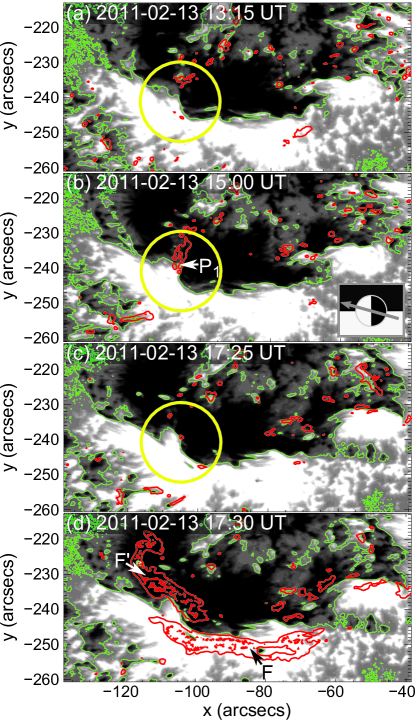
Figure 7: Onset processes for solar flares in AR NOAA 11158 observed by Hinode/SOT. Gray scale (black, negative; white, positive) represents the Stokes-V/I signal in the Na I 5896 Å line. Red contours indicate the emission of the Ca II H line, and green lines represent the polarity inversion line (PIL). Observation times are shown for each subset. Subset at the lower right corner of (b) illustrates the typical RS structure with counterclockwise rotating sheared field.

The second event, which can be explained by the RS-type trigger model, is the M6.6-class flare observed in AR NOAA 11158 at 17:28 UT on February 13, 2011 (Fig. 7). The vector magnetogram (SOT/SP) indicates that the magnetic field in this region was also extensively twisted (more than $75^{\circ}$) in a counterclockwise direction. This counterclockwise twist, which corresponds to the preloaded positive magnetic helicity, is consistent with the sheared structure of the flare ribbons (Fig. 7d).

Here we emphasize that an inverse S-shaped structure of the PIL, in which positive and negative polarity regions edge into each other, was formed in the region denoted by yellow circles in Figs. 7a-7c between 13:15 UT and 15:00 UT. On the center of this region, the PIL is running north-south, whereas the overall PIL generally is running east-west. Therefore, it is highly likely that magnetic field crossing the inverse S-shaped PIL is reversely directed compared with the large scale sheared magnetic field, and that the RS-type configuration is formed as illustrated in the subset at the lower right corner of Fig. 7b.

In fact, the brightening of the Ca II H line (P₁ in Fig. 7b) was observed since 15:00 UT in this area. This preflare brightening can be attributed to heating of the current sheet between the pre-existing sheared field and magnetic field of RS, which corresponds to c in Fig. 4b. Immediately after the onset of the flare, sheared ribbons F and F’ appeared as a center on the inverse S-shaped PIL (Fig. 7d). The ribbon structure is highly consistent with the simulation result such that the feet of the twisted ropes (F and F’ in Fig. 4) and post-flare arcades (R and R’) combined to create elongated sheared ribbons on both sides of the RS field region (Fig. 4h).

Furthermore, it is worthwhile to note that the preflare brightening (P₁ in Fig. 7) was weakened before the onset of the flare (see Fig. 7c). In the simulation, the electric current intensity on the current sheet c was weakened just prior to eruption of twisted ropes (see Fig. 4d). This weakening resulted from the reconnection on the current sheet v, because the reconnection ejected downward the shear-free field, which prevented contact between the pre-existing sheared field and the field of RS. The agreement of the observation and simulation results indicates that the weakening of preflare brightening on the RS-like region could be regarded as a precursor of flare onset.

From the magnetic structure and evolution of preflare and flare ribbons, we can conclude that this event is consistent with the RS-type trigger scenario. The formation process of the inverse S-shaped PIL in this region is an interesting subject and we are analyzing the cause of the strucutre. The detail results of analysis will be reported elsewhere.

5 Discussion and Conclusion

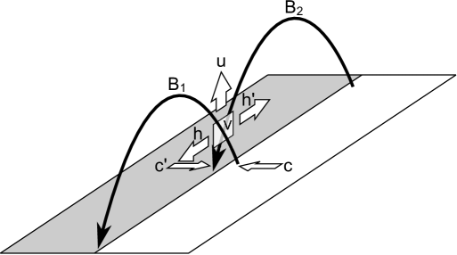
Figure 8: Illustration of the three different flows u, h-h’, and c-c’, which may cause the formation of a vertical current sheet v and magnetic reconnection between two sheared magnetic loops B₁ and B₂ on the polarity inversion line (PIL).

The results shown in the previous section indicate that events indeed occurred, which are described by the following two scenarios: Scenario 1 involves an eruption-induced reconnection process triggered by an OP-type magnetic field, and Scenario 2 is a reconnection-induced eruption process triggered by an RS-type magnetic field. Here, we examine the reason for existence of both scenarios. It is explicable in terms of the topology of the magnetic field. In both scenarios, flare reconnection on a vertical current sheet is caused by the diverging flows that remove magnetic flux and plasma from the reconnection site. This mechanism corresponds to the “pull” mode in reconnection experiments performed in laboratories (Yamada, 1999). As shown in Fig. 8, two different types of divergent flows are able to form thin current sheet v between two sheared magnetic loops B₁ and B₂. One divergent flow is a vertical (upward) flow above the PIL (u in Fig. 8), and the other is a horizontal flow along the PIL (h and h’). They correspond to the preflare flows that trigger flare reconnection in Scenarios 1 and 2, respectively. Because a divergent flow can flow either in the vertical or horizontal direction, two different scenarios exist.

On the other hand, the converging flow (c and c’) can also form a vertical current sheet and may drive flare reconnection, which corresponds to the “push” mode in reconnection experiments (Yamada, 1999). In fact, the converging flow on the solar surface is believed to play the role of a trigger in the flux cancellation (FC) model (Inhester et al., 1992; Priest et al., 1994; Amari et al., 2003a). Therefore, from the perspective of magnetic topology, we can conclude that these three scenarios (Scenarios 1 and 2 proposed in this paper as well as the reconnection scenario caused by the converging flow) can all apply to the triggering of solar flares.

The classification of the PIL morphology in flaring sites is a promising technique used to examine the applicability of each scenario because each scenario requires different structures of PIL as illustrated in Fig. 5. Scenario 1 requires an OP-type disturbance to the PIL (Fig. 5a). On the other hand, the inverse S-shaped PIL (RS+ in Fig. 5b) and the S-shaped PIL (RS$-$ in Fig. 5b) are the notable signature of the RS structures when the large-scale sheared field is positive (counterclockwise rotated) and negative (clockwise rotated), respectively, although an RS structure without a disturbed PIL is possible (Kusano et al., 2004). In fact, such types of the PIL morphology have been observed in several flare-productive active regions; e.g. ARs NOAA 6659 (Fig. 1a of Zirin & Wang (1993)) and NOAA 9026 (Fig. 4q of Kurokawa et al. (2002)) for an OP-type morphology, AR NOAA 9026 (Fig. 4k of Kurokawa et al. (2002)) for an RS-type morphology.

On the other hand, the FC model caused by the converging flow does not require any disturbances to the PIL if positive and negative magnetic fluxes cancel each other. However, because the emergence of a magnetic element in the flaring site is often associated with the cancellation of magnetic flux (Wang & Shi, 1993), we should carefully recognize the structure of flare triggering. Our analyses suggest that a high cadence (less than a couple of minutes) of preflare brightening observation in the chromospheric lines such as Ca II H is a powerful tool to recognize preflare processes. The statistical study of various solar eruptions will explain the applicability of each scenario to the onset of solar flare and CMEs.

Our study suggests that solar flares and CMEs are triggered by magnetic disturbances in regions where magnetic shear has stored free energy rather than originating in phenomena that inevitably occur as a consequence of free energy storage; i.e., both magnetic shear (or magnetic helicity) and “proper” disturbance of the magnetic field are necessary for the occurrence of solar flares and CMEs. This conclusion implies that the lead time for flare and CME forecasting is limited by the time scale of changes in small magnetic elements that work as a trigger. Our analysis of the two events suggests a lead time shorter than several hours. Longer forecasting can be difficult and may be possible only in a probabilistic manner.

While the simulations indicate that the orientation of a small magnetic element that perturbs the sheared magnetic structure is crucial for triggering flares and CMEs, it is highly likely that the size and location (displacement from PIL) of magnetic perturbation are also important. The results of more advanced simulations to determine the significance of these parameters will be published elsewhere.

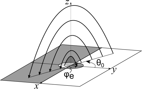
Figure 1: Illustration of simulation setup. Curved solid lines with arrows correspond to magnetic field lines in the preexisting force-free field and the small scale injected field, which rotate $\theta_{0}$ and $\varphi_{e},$ respectively, with respect to the large scale potential field. White and gray areas on the bottom surface indicate positive and negative magnetic polarity regions.

Figure 2: Summary of simulations for $B_{e}=2,$ $r_{e}=0.13,$ $\tau_{e}=20,$ $v_{e}=6.7\times 10^{-3},$ $y_{e}=0$ on parameter space of $\varphi_{e}$ and $\theta_{0}.$ Different marks (squares and diamonds) represent the types of dynamics, and contours show the maximum total kinetic energy produced by eruption ($E_{k}$). Squares indicate that no eruption has occurred at the corresponding parameter; diamonds indicate the appearance of eruptions at each parameter. Pink and blue diamonds indicate eruption-induced reconnection and reconnection-induced eruption processes, respectively. The yellow diamond corresponds to a special case in which the potential field collapses because of reconnection with the small scale injected field, which exhibits a completely antiparallel polarity compared with the initial potential field. Right hand and top subsets illustrate the initial sheared field and orientation of injected small bipole field, respectively, in which white and black areas indicate positive and negative polarity and arrows represent the horizontal component of the magnetic field.

Figure 3: Simulation result for $\varphi_{e}=180^{\circ}$ and $\theta_{0}=77.5^{\circ}$, in which the OP-type of magnetic structure causes the eruption-induced reconnection dynamics. Each subset represent a birds eye view (a, c, e-h), top view (b), and enlarged side view (d) of the magnetic field at different times. Green tubes represent magnetic field lines with connectivity that differs from the initial state. Selected magnetic fields in the initial state and those retaining the initial connectivity are plotted by blue tubes in (a) and (d), respectively. Red contours correspond to intensive current layers in which $|\nabla\times\mathbf{B}|>40.$ Gray scales (white, positive; black, negative) on the bottom plane indicate the distribution of the $z$ component of magnetic field $B_{z}.$ Other parameters are $B_{e}=2$, $r_{e}=0.13,$ $\tau_{e}=20,$ $v_{e}=6.7\times 10^{-3},$ and $y_{e}=0.$

Figure 4: Simulation result for $\varphi_{e}=270^{\circ}$ and $\theta_{0}=77.5^{\circ}$, in which the RS-type of magnetic structure causes the reconnection-induced eruption dynamics. Each subset represents a birds eye view (a, c, and e-h) and enlarged side views (b and d) of the magnetic field at different times. Green tubes represent magnetic field lines with connectivity that differs from the initial state. Selected magnetic fields in the initial state and those retaining the initial connectivity are plotted by blue tubes in (a) and blue and sky-blue tubes in (b-d), respectively. Red arrows in (b-d) represent the typical flow directions. The format and other parameters are same as those described in Fig. 3.

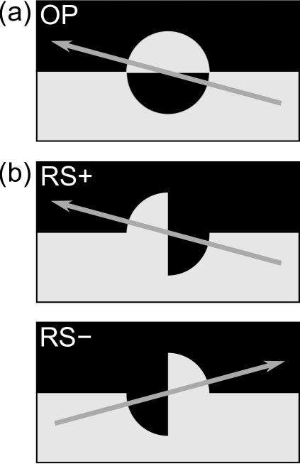
Figure 5: Schematic diagram of top view of (a) OP and (b) RS-type magnetic structures. Arrows indicate the large scale sheared magnetic field, and black and white parts correspond to the negative and positive polarity regions. The chirality of PIL disturbance in the RS-type structure is changed depending on the sign of magnetic shear; RS+ for positive shear (counterclockwise rotation) and RS$-$ for negative shear (clockwise rotation).

Figure 6: Onset processes for solar flares in AR NOAA 10930 observed by Hinode/SOT (a-c, e, g, and i), and soft X-ray images obtained with the Hinode/XRT (d, f, h, and j). Gray scale in the SOT data represents the Stokes-V/I signal of the Fe I 6302 Å line, which indicates circular polarization corresponding to the line-of-sight component of the magnetic field (black, negative; white, positive). Red contours indicate the emission of the Ca II H line. Green lines on the SOT data and gray lines on the XRT data represent the polarity inversion line (PIL) in the central region. Observation times are shown for each subset. Subset at the lower right corner of (b) illustrates the typical OP-type magnetic structure with clockwise rotating sheared field.

References

- Abramenko & Yurchyshyn (2010) Abramenko, V., & Yurchyshyn, V. 2010, ApJ, 722, 122
- Amari et al. (2003a) Amari, T., Luciani, J. F., Aly, J. J., Mikic, Z., & Linker, J. 2003, ApJ, 585, 1073
- Amari et al. (2003b) Amari, T., Luciani, J. F., Aly, J. J., Mikic, Z., & Linker, J. 2003, ApJ, 595, 1231
- Antiochos et al. (1999) Antiochos, S. K., DeVore, C. R., & Klimchuk, J. A. 1999, ApJ, 510, 485
- Archontis & Hood (2012) Archontis, V. & Hood, A. W. 2012, A&A, 537, A62
- Canfield et al. (1999) Canfield, R. C., Hudson, H. S., & McKenzie, D. E. 1999, Geophys. Res. Lett., 26, 627
- Carmichael (1964) Carmichael, H. 1964, NASA Special Publ., 50, 451
- Chandra et al. (2010) Chandra, R., Pariat, E., Schmieder, B., Mandrini, C. H., & Uddin, W. 2010, Sol. Phys., 261, 127
- Chen (1996) Chen, J. 1996, J. Geophys. Res., 101, 27499
- Chen & Shibata (2000) Chen, P. F. & Shibata, K. 2000, ApJ, 545, 524
- Cheng et al. (2010) Cheng, X., Ding, M. D., & Zhang, J. 2010, ApJ, 712, 1302
- Chifor, et al. (2007) Chifor, C., Tripathi, D., Mason, H. E., & Dennis, B. R. 2007, A&A, 472, 967
- Démoulin & Aulanier (2010) Démoulin, P., & Aulanier, G. 2010, ApJ, 718, 1388
- Fan & Gibson (2004) Fan, Y., & Gibson, S. E. 2004, ApJ, 609, 1123
- Fan & Gibson (2007) Fan, Y., & Gibson, S. E. 2007, ApJ, 668, 1232
- Feynman & Martin (1995) Feynman, J., & Martin, S. F. 1995, J. Geophys. Res., 100, 3355
- Forbes (2000) Forbes, T. G. 2000, J. Geophys. Res., 105, 23153
- Forbes & Priest (1995) Forbes, T. G. & Priest, E. R. 1995, ApJ, 446, 377
- Golub et al. (2007) Golub, L., Deluca, E., Austin, G., et al. 2007, Sol. Phys., 243, 63
- Green et al. (2011) Green, L. M., Kliem, B., & Wallace, A. J. 2011, A&A, 526, A2
- Hagyard, et al. (1984) Hagyard, M. J., Smith, Jr., J. B., Teuber, D. & Wewst, E. A. 1984, Sol. Phys., 91, 115
- Hanaoka (1997) Hanaoka, Y. 1997, Sol. Phys., 173, 319
- Heyvaerts, Priest & Rust (1977) Heyvaerts, J., Priest, E. R., & Rust, D. M., 1997, ApJ, 216, 123
- Hirayama (1974) Hirayama, T. 1974, Sol. Phys., 34, 323
- Inhester et al. (1992) Inhester, B., Birn, J., & Hesse, M. 1992, Sol. Phys., 138, 257
- Kliem & Török (2006) Kliem, B. & Török, T. 2006, Physical Review Letters, 96, 255002
- Kopp & Pneuman (1976) Kopp, R. A., & Pneuman, G. W. 1976, Sol. Phys., 50, 85
- Kosugi et al. (2007) Kosugi, T., Matsuzaki, K., Sakao, T., et al. 2007, Sol. Phys., 243, 3
- Kubo et al. (2007) Kubo, M., Yokoyama, T., Katsukawa, Y., et al. 2007, PASJ, 59, 779
- Kurokawa et al. (2002) Kurokawa, H., Wang, T., & Ishii, T. T. 2002, ApJ, 572, 598
- Kusano et al. (1995) Kusano, K., Suzuki, Y., & Nishikawa, K. 1995, ApJ, 441, 942
- Kusano et al. (2004) Kusano, K., Maeshiro, T., Yokoyama, T., & Sakurai, T. 2004, ApJ, 610, 537
- Kusano (2005) Kusano, K. 2005, ApJ, 631, 1260
- Leka & Barnes (2007) Leka, K. D. & Barnes, 2007, ApJ, 656, 1173
- Low (1977) Low, B. C. 1977, ApJ, 212, 234
- Mikic & Linker (1994) Mikic, Z., & Linker, J. A. 1994, ApJ, 430, 898
- Moore & Roumeliotis (1992) Moore, R. L. & Roumeliotis, G. 1992, IAU Colloq. 133: Eruptive Solar Flares, 399, 69
- Moore et al. (2001) Moore, R. L., Sterling, A. C., Hudson, H. S., & Lemen, J. R. 2001, ApJ, 552, 833
- Moore et al. (2011) Moore, R. L., Sterling, A. C., Gary, G. A., Cirtain, J.W., & Falconer, D. A. 2011, Space Sci. Rev., 160, 73
- Park et al. (2010) Park, S.-H., Chae, J., Jing, J., Tan, C., & Wang, H. 2010, ApJ, 720, 1102
- Priest et al. (1994) Priest, E. R., Parnell, C. E., & Martin, S. F. 1994, ApJ, 427, 459
- Priest & Forbes (2002) Priest, E. R. & Forbes, T. G. 2002, A&A Rev., 10, 313
- Romano & Zuccarello (2011) Romano, P., & Zuccarello, F. 2011, A&A, 535, A1
- Rust & Kumar (1996) Rust, D. M., & Kumar, A. 1996, ApJ, 464, L199
- Schmieder et al. (1994) Schmieder, B., Hagyard, M. J., Guoxiang, A., et al. 1994, Sol. Phys., 150, 199
- Schrijver (2007) Schrijver, C. J. 2007, ApJ, 655, L117
- Shibata & Magara (2011) Shibata, K. & Magara, T. 2011, Living Reviews in Solar Physics 8, 6
- Sterling & Moore (2004) Sterling, A. C., & Moore, R. L. 2004, ApJ, 602, 1024
- Sturrock (1966) Sturrock, P. A. 1966, Nature, 211, 695
- Titov et al. (1993) Titov, V. S., Priest, E. R., & Demoulin, P. 1993, A&A, 276, 564
- Török & Kliem (2005) Török, T., & Kliem, B. 2005, ApJ, 630, L97
- Tsuneta et al. (2008) Tsuneta, S., Ichimoto, K., Katsukawa, Y., et al. 2008, Sol. Phys., 249, 167
- van Ballegooijen & Martens (1989) van Ballegooijen, A. A., & Martens, P. C. H. 1989, ApJ, 343, 971
- Vemareddy et al. (2012) Vemareddy, P., Ambastha, A., Maurya, R. A., & Chae, J. 2012, arXiv:1202.5195, submitted to ApJ
- Wallace et al. (2010) Wallace, A. J., Harra, L. H., van Driel-Gesztelyi, L., Green, L. M., & Matthews, S. A. 2010, Sol. Phys., 267, 361
- Wang & Shi (1993) Wang, J., & Shi, Z. 1993, Sol. Phys., 143, 119
- Wang et al. (2004) Wang, J., Zhou, G., & Zhang, J. 2004, ApJ, 615, 1021
- Welsch et al. (2011) Welsch, B. T., Christe, S., & McTiernan, J. M. 2011, Sol. Phys., 274, 131
- Williams et al. (2005) Williams, D. R., Török, T., Démoulin, P., van Driel-Gesztelyi, L., & Kliem, B. 2005, ApJ, 628, L163
- Yamada (1999) Yamada, M. 1999, J. Geophys. Res., 104, 14529
- Zhang (2001) Zhang, H. 2001, ApJ, 557, L71
- Zhang et al. (2001) Zhang, J., Wang, J., Deng, Y., & Wu, D. 2001, ApJ, 548, L99
- Zirin & Wang (1993) Zirin, H., & Wang, H. 1993, Nature, 363, 426