Thermal entanglement in exactly solvable Ising-XXZ diamond chain structure

Abstract

Most quantum entanglement investigations are focused on two qubits or some finite (small) chain structure, since the infinite chain structure is a considerably cumbersome task. Therefore, the quantum entanglement properties involving an infinite chain structure is quite important, not only because the mathematical calculation is cumbersome but also because real materials are well represented by an infinite chain. Thus, in this paper we consider an entangled diamond chain with Ising and anisotropic Heisenberg (Ising-XXZ) coupling. Two interstitial particles are coupled through Heisenberg coupling or simply two-qubit Heisenberg, which could be responsible for the emergence of entanglement. These two-qubit Heisenberg operators are interacted with two nodal Ising spins. An infinite diamond chain is organized by interstitial- interstitial and nodal-interstitial (dimer-monomer) site couplings. We are able to get the thermal average of the two-qubit operator, called the reduced two-qubit density operator. Since these density operators are spatially separated, we could obtain the concurrence (entanglement) directly in the thermodynamic limit. The thermal entanglement (concurrence) is constructed for different values of the anisotropic Heisenberg parameter, magnetic field and temperature. We also observed the threshold temperature via the parameter of anisotropy, Heisenberg and Ising interaction, external magnetic field, and temperature.

I Introduction

Quantum entanglement is one of the most attractive types of correlations that can be shared only among quantum systems AmicoHorod . In recent years, many efforts have been devoted to characterize qualitatively and quantitatively the entanglement properties of condensed matter systems, which are the natural candidate to apply for quantum communication and quantum information. In this sense, it is very important to study the entanglement of solid state systems such as spin chains qubit-Heisnb . The Heisenberg chain is one of the simplest quantum systems, which exhibits entanglement; due to the Heisenberg interaction it is not localized in the spin system.

In the last decade, several diamond chain structures have been discussed. It is interesting to consider the quantum antiferromagnetic Heisenberg model on a generalized diamond chain, which describes real materials such as $\mathrm{Cu_{3}(CO_{3})_{2}(OH)_{2}}$, known as natural azurite. Honecker et al. honecker studied the dynamic and thermodynamic properties for this model. In addition, Pereira et al. Pereira08 ; pereira09 investigated the magnetization plateau of delocalized interstitial spins, as well as magnetocaloric effect in kinetically frustrated diamond chains. More recently, Lisnii lisnii studied a distorted diamond Ising-Hubbard chain, and that the model also reveals the geometrical frustration. Thermodynamics of the Ising-Heisenberg model on a diamond-like chain was widely discussed in the Refs canova06 ; vadim ; valverde ; lisnii-11 .

The motivation for the study of the Ising and anisotropic Heisenberg (Ising-XXZ) model on a diamond chain, according to experiments of the natural mineral azurite, theoretical calculations of the Ising-XXZ model, as well as the experimental result of the dimer (interstitial sites) exchange parameter is based on a number of recent works. The 1/3 magnetization plateau and the double peaks both in the magnetic susceptibility and specific heat were observed in the experimental measurements rule ; kikuchi . It should be noticed that the dimer (interstitial sites) exchange is much stronger than those nodal sites. Various types of theoretical Heisenberg-model approximate methods were proposed: renormalization of the density matrix renormalization group of the transfer matrix, density functional theory, high-temperature expansion, variational mean-field-like treatment based on the Gibbs-Bogoliubov inequality, and Lanczos diagonalization on a diamond chain to explain the experimental measurements (magnetization plateau and the double peaks) in the natural mineral azurite honecker-lauchli . The localizable entanglement (LE) has been calculated for ground states of arbitrary Hamiltonians numerically by making use of the density renormalization group formalism and exhibited characteristic features at a quantum phase transition. The LE is completely characterized by the maximal connected correlation function for ground states of spin-1/2 systems martin . All of these theoretical studies are approximate. There is another possibility. Since dimer interaction is much higher than the rest, it can be represented as an exactly solvable Ising-Heisenberg model. In addition, experimental data on the magnetization plateau coincide with the approximation Ising-Heisenberg model canova06 ; Pereira08 ; ananikian ; chakh .

Several studies have been done on the threshold temperature for the pairwise thermal entanglement in the Heisenberg model with a finite number of qubits. Thermal entanglement of the isotropic Heisenberg chain of spin has been studied in the absence wang and in the presence of an external magnetic field X-Wang ; arnesen . The pairwise thermal entanglement of nearest-neighbor qubits is independent of the sign of exchange constants and the sign of magnetic fields in the XX even-number qubit ring with a magnetic field. The thermal entanglement in Heisenberg XX decreases with increasing temperature and the threshold temperature value $T_{th}$ is independent of the external magnetic field. Although in some references the threshold temperature $T_{th}$ is called the quantum critical temperature, here we call it the threshold temperature to avoid misunderstanding with the magnetic phase transition temperature.

It is quite relevant to study the thermal entanglement of the Ising-XXZ on diamond chain, as Ananikian et al. ananikian ; chakh have discussed the thermal entanglement of the Ising-Heisenberg chain in the isotropic limit in the cluster approach. The paper is organized as follows: In Sec. II we present the Ising-XXZ model on diamond chain. We obtain the exact solution of the model via the transfer-matrix approach and its dimer (two-qubit) reduced density operator in Sec. III. In Sec. IV, we discuss the thermal entanglement of the Heisenberg reduced density operator of the model, such as concurrence and threshold temperature. Finally, concluding remarks are given in Sec. V.

II Ising-XXZ diamond Hamiltonian

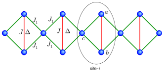
Figure 1: (Color online) Schematic representation of XXZ-Ising diamond chain. Red line represents the quantum bipartite coupling.

In this work, we study the Ising-XXZ model with mixed nodal Ising spins and interstitial anisotropic Heisenberg spins in the presence of an external magnetic field on a diamond-like chain. The thermodynamic properties were previously discussed in Refs. canova06 ; valverde ; lisnii ; vadim . A diamond-like chain is schematically illustrated in Fig 1. The Hamiltonian operator can be expressed as follows:

$$\mathcal{H}= \sum_{i=1}^{N}J\left(\boldsymbol{S}_{a,i},\boldsymbol{S}_{b,i}\right)_{\Delta}+J_{1}\left(S_{a,i}^{z}+S_{b,i}^{z}\right)\left(\mu_{i}+\mu_{i+1}\right)+$$

$$-h_{0}\left(S_{a,i}^{z}+S_{b,i}^{z}\right)-\frac{h}{2}\left(\mu_{i}+\mu_{i+1}\right),$$ (1)

where $\left(\boldsymbol{S}_{a,i},\boldsymbol{S}_{b,i}\right)_{\Delta}=S_{a,i}^{x}S_{b,i}^{x}+S_{a,i}^{y}S_{b,i}^{y}+\Delta S_{a,i}^{z}S_{b,i}^{z}$ corresponds to the interstitial anisotropic Heisenberg spins coupling ($J$ and $\Delta$), while the nodal-interstitial (dimer-monomer) spins are representing by Ising-type exchanges ($J_{1}$). The Hamiltonian also includes a longitudinal external magnetic field $h_{0}$ acting on Heisenberg spins and a magnetic $h$ acting on Ising spins. For convenience, we will consider the case $h_{0}=h$.

The quantum Heisenberg spin coupling can be expressed using matrix notation. We have

$$\left(\boldsymbol{S}_{a,i},\boldsymbol{S}_{b,i}\right)_{\Delta}=\left[\begin{array}[]{cccc}\frac{\Delta}{4}&0&0&0\\ 0&-\frac{\Delta}{4}&\frac{1}{2}&0\\ 0&\frac{1}{2}&-\frac{\Delta}{4}&0\\ 0&0&0&\frac{\Delta}{4}\end{array}\right]$$ (2)

and

$$S_{a,i}^{z}+S_{b,i}^{z}=\left[\begin{array}[]{cccc}1&0&0&0\\ 0&0&0&0\\ 0&0&0&0\\ 0&0&0&-1\end{array}\right].$$ (3)

We obtain the following eigenvalues by diagonalization of the two-qubit Heisenberg (dimer) exchange and by assuming fixed values for $\mu_{i}$ and $\mu_{i+1}$:

$$\mathcal{E}_{1}(\mu_{i},\mu_{i+1})= \frac{J\Delta}{4}+\left(J_{1}-\frac{h}{2}\right)\left(\mu_{i}+\mu_{i+1}\right)-h,$$

$$\mathcal{E}_{2}(\mu_{i},\mu_{i+1})= \frac{J}{2}-\frac{J\Delta}{4}-\frac{h}{2}\left(\mu_{i}+\mu_{i+1}\right),$$

$$\mathcal{E}_{3}(\mu_{i},\mu_{i+1})= -\frac{J}{2}-\frac{J\Delta}{4}-\frac{h}{2}\left(\mu_{i}+\mu_{i+1}\right),$$

$$\mathcal{E}_{4}(\mu_{i},\mu_{i+1})= \frac{J\Delta}{4}-\left(J_{1}+\frac{h}{2}\right)\left(\mu_{i}+\mu_{i+1}\right)+h,$$ (4)

where their corresponding eigenstate in terms of standard basis $\{|\uparrow\uparrow\rangle,|\downarrow\downarrow\rangle,|\uparrow\downarrow\rangle,|\downarrow\uparrow\rangle\}$ are given respectively by

$$|\varphi_{1}\rangle= |\uparrow\uparrow\rangle,$$ (5)

$$|\varphi_{2}\rangle= \frac{1}{\sqrt{2}}\left(|\uparrow\downarrow\rangle+|\downarrow\uparrow\rangle\right),$$ (6)

$$|\varphi_{3}\rangle= \frac{1}{\sqrt{2}}\left(|\uparrow\downarrow\rangle-|\downarrow\uparrow\rangle\right),$$ (7)

$$|\varphi_{4}\rangle= |\downarrow\downarrow\rangle.$$ (8)

In quantum information the states $|\varphi_{2}\rangle$ and $|\varphi_{3}\rangle$ are known as the "magic basis" or Bell state, where two-qubit Heisenberg are maximally entangled. These states are responsible for the rise of entanglement at finite temperature.

In order to study the two-qubit entanglement, we use the concurrence wootters ; hill , which is defined by

$$\mathcal{C}=|\langle\varphi_{i}|\tilde{\varphi}_{i}\rangle|,$$ (9)

where $|\tilde{\varphi}_{i}\rangle$ means the spin-flip state. Therefore, the concurrence $\mathcal{C}$ will be for states $|\varphi_{2}\rangle$ and $|\varphi_{3}\rangle$, which corresponds to qubits that are maximally entangled. If the states $|\varphi_{1}\rangle$ and $|\varphi_{4}\rangle$ have no concurrence ($\mathcal{C}=0$), that means the qubits are unentangled. Later we give the definition of entanglement in more detail.

II.1 Zero temperature phase diagram of entangled state

In this section we study the phase diagram of the entangled states, similar to the magnetic phase previously discussed in Refs. canova06 ; valverde , where it was observed three magnetic states, a frustrated (FRU) state, a ferrimagnetic (FIM) state, and a ferromagnetic (FM) state. Although we only have two states (entangled and unentangled), we discuss here the entangled region which is closely related to the magnetic states. It can be expressed the following states:

$$\mid ENT\rangle =\overset{N}{\underset{i=1}{\prod}}\mid\varphi_{3}\rangle_{i}\otimes\mid\mu\rangle_{i},$$ (10)

$$\mid UFI\rangle =\overset{N}{\underset{i=1}{\prod}}\mid\varphi_{1}\rangle_{i}\otimes\mid-\rangle_{i},$$ (11)

$$\mid UFM\rangle =\overset{N}{\underset{i=1}{\prod}}\mid\varphi_{1}\rangle_{i}\otimes\mid+\rangle_{i},$$ (12)

where $\mid\mu\rangle_{i}$ stands for arbitrary values ($\mu=\pm 1/2$) of the nodal spin in the $i$-th block.

According to the Bell states given in eqs.(6) and (7), at zero temperature the entangled (ENT) state is fully spanned in the frustrated state for zero magnetic field, while the ferrimagnetic and ferromagnetic state is spanned by unentangled states denoted by UFI and UFM respectively.

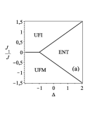
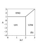
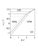
Figure 2: Phase diagrams of entangled state at zero temperature. The entangled state in frustrated phase denoted by ENT, whereas the entangled state in quantum ferrimagnetic phase we denote by ENQ. The unentangled state in ferrimagnetic phase (UFI) and unentangled ferromagnetic (UFM) states.

In Fig. 2(a) we plot the phase diagram $\Delta$ versus $J_{1}/J$ at zero temperature for $h/J=h_{0}/J=0$ , where the ground-state energy of the entangled state is $E_{ENT}=-\frac{1}{2}-\frac{\Delta}{4}$, while for the unentangled state (ferrimagnetic state) it is $E_{UFI}=-\frac{J_{1}}{J}+\frac{\Delta}{4}$, and for the unentangled state (ferromagnetic state) it is given by $E_{UFM}=\frac{J_{1}}{J}+\frac{\Delta}{4}$. The phase boundary between UFI and UFM is simply $J_{1}/J=0$, and the phase boundary between the UFI and ENT states is given by $(\frac{J_{1}}{J}=\frac{\Delta}{2}+\frac{1}{2})$, while the phase boundary between UFM and ENT (frustrated) state is given by $(\frac{J_{1}}{J}=-\frac{\Delta}{2}-\frac{1}{2})$.

In Fig. 2(b) we plot the phase diagram $\Delta$ versus $h/J$ at zero temperature for $J_{1}/J=1$ and $h/J=h_{0}/J$, where the eigenvalues for the unentangled state UFM is given by $E_{UFM}=1+\frac{\Delta}{4}-\frac{3h}{2J}$, while for the entangled state (quantum ferrimagnetic state) denoted by $\mid ENQ\rangle=\overset{N}{\underset{i=1}{\prod}}\mid\varphi_{3}\rangle_{i}\otimes\mid+\rangle_{i},$ and its eigenvalues is $E_{ENQ}=-\frac{1}{2}-\frac{\Delta}{4}-\frac{h}{2J}$. We also have the unentangled state UFI whose eigenvalue becomes $E_{UFI}=-1+\frac{\Delta}{4}-\frac{h}{2J}$. The phase boundary between UFM and UFI is given by $h/J=2$, whereas between the ENQ and UFI states it is limited by $\Delta=1$, while for the ENQ and UFM states we have $\Delta=\frac{2h}{J}-3$.

Finally, in Fig. 2(c) we illustrate the phase diagram $J_{1}/J$ versus $h/J$ at zero temperature for $\Delta=1$ and $h/J=h_{0}/J$, where the eigenvalues are given by $E_{ENQ}=-\frac{3}{4}-\frac{h}{2J}$ , $E_{UFI}=\frac{1}{4}-\frac{J_{1}}{J}-\frac{h}{2J}$ and $E_{UFM}=\frac{1}{4}+\frac{J_{1}}{J}-\frac{3h}{2J}$. The phase boundary between the ENQ and UFI states is limited by $J_{1}/J=1$, while the boundary between UFI and UFM is given by $J_{1}=h/2$, and between the ENQ and UFM states the boundary follows the curve $\frac{J_{1}}{J}=\frac{h}{J}-1$. The doted line corresponds to the phase diagram for $\Delta=0.5$, whereas the dashed line represent the phase diagram for $\Delta=1.5$.

However, entangled states will change with increasing temperature. This will be discussed in Sec. IV.

III The partition function and density operator

With the aim of studying any thermal quantities, we first need to obtain a partition function on a diamond chain. As mentioned earlier Fisher ; Syozi ; phys-A-09 , this model can be solved exactly through a decoration transformation and transfer-matrix approach baxter-book . In order to summarize this approach we will define the following operator as a function of Ising spin particles $\mu$ and $\mu^{\prime}$,

$$\varrho(\mu,\mu^{\prime})=\mathrm{e}^{-\beta H_{ab}(\mu,\mu^{\prime})},$$ (13)

where $H_{ab}(\mu,\mu^{\prime})$ corresponds to the $r$th-block Hamiltonian (1) (without summations), which depends on the neighboring Ising spins $\mu$ and $\mu^{\prime}$. Alternatively the operator (13) could be written in terms of two-qubit operator eigenvalues (4), which is

$$\varrho(\mu,\mu^{\prime})=\sum_{i=1}^{4}\mathrm{e}^{-\beta\varepsilon_{i}(\mu,\mu^{\prime})}|\varphi_{i}\rangle\langle\varphi_{i}|.$$ (14)

Straightforwardly, we can obtain the Boltzmann factor by tracing out over the two-qubit operator,

$$w(\mu,\mu^{\prime})=\mathrm{tr}_{ab}\left(\varrho(\mu,\mu^{\prime})\right)=\sum_{i=1}^{4}\mathrm{e}^{-\beta\varepsilon_{i}(\mu,\mu^{\prime})},$$ (15)

where the Ising-XXZ diamond chain partition function can be written in terms of Boltzmann factors,

$$Z_{N}=\sum_{\{\mu\}}w(\mu_{1},\mu_{2})\ldots w(\mu_{N},\mu_{1}).$$ (16)

Using the transfer-matrix notation, we can write the partition function of the diamond chain straightforwardly by $Z_{N}=\mathrm{tr}\left(W^{N}\right),$ where the transfer-matrix is expressed as

$$W=\left[\begin{array}[]{cc}w(\frac{1}{2},\frac{1}{2})&w(\frac{1}{2},-\frac{1}{2})\\ w(-\frac{1}{2},\frac{1}{2})&w(-\frac{1}{2},-\frac{1}{2})\end{array}\right],$$ (17)

where the transfer matrix elements are denoted by $w_{++}\equiv w(\frac{1}{2},\frac{1}{2})$, $w_{+-}\equiv w(\frac{1}{2},-\frac{1}{2})$ and $w_{--}\equiv w(-\frac{1}{2},-\frac{1}{2})$.

After performing the diagonalization of the transfer matrix (17), the eigenvalues are

$$\Lambda_{\pm}=\frac{w_{++}+w_{--}\pm Q}{2},$$ (18)

assuming that $Q=\sqrt{\left(w_{++}-w_{--}\right)^{2}+4w_{+-}^{2}}$. Therefore, the partition function for finite chain under periodic boundary conditions is given by

$$Z_{N}=\Lambda_{+}^{N}+\Lambda_{-}^{N}.$$ (19)

In the thermodynamic limit the partition function will be simplified, which results in $Z_{N}=\Lambda_{+}^{N}$. It is worth noticing that this result was widely used in Refs. canova06 ; valverde ; vadim ; lisnii .

III.1 Two-qubit operator

In order to calculate the two-qubit Heisenberg operator bonded by Ising particles $\mu$ and $\mu^{\prime}$, we assume that the Ising spin of the particle is fixed. Thus, the qubits operator elements in the natural basis becomes

$$\varrho=\left[\begin{array}[]{cccc}\varrho_{1,1}&0&0&0\\ 0&\varrho_{2,2}&\varrho_{2,3}&0\\ 0&\varrho_{3,2}&\varrho_{3,3}&0\\ 0&0&0&\varrho_{4,4}\end{array}\right],$$ (20)

where the elements of the two-qubit operator are given by

$$\varrho_{1,1}(\mu,\mu^{\prime})= \mathrm{e}^{-\beta\varepsilon_{1}(\mu,\mu^{\prime})},$$

$$\varrho_{2,2}(\mu,\mu^{\prime})= \frac{1}{2}\left(\mathrm{e}^{-\beta\varepsilon_{2}(\mu,\mu^{\prime})}+\mathrm{e}^{-\beta\varepsilon_{3}(\mu,\mu^{\prime})}\right),$$

$$\varrho_{2,3}(\mu,\mu^{\prime})= \frac{1}{2}\left(\mathrm{e}^{-\beta\varepsilon_{2}(\mu,\mu^{\prime})}-\mathrm{e}^{-\beta\varepsilon_{3}(\mu,\mu^{\prime})}\right),$$

$$\varrho_{4,4}(\mu,\mu^{\prime})= \mathrm{e}^{-\beta\varepsilon_{4}(\mu,\mu^{\prime})}.$$ (21)

The thermal average for each two-qubit Heisenberg operator will be used to construct the reduced density operator.

III.2 Reduced density operator and transfer matrix approach

We will perform the reduced density operator bounded by Ising particles along a diamond chain. We can proceed by tracing out over all Heisenberg spins and Ising spins except at the rth block in Heisenberg spins on a diamond chain. Using the transfer-matrix approach, we are able to write the reduced density operator by the following expression

$$\rho_{i,j}= \frac{1}{Z_{N}}\sum_{\{\mu\}}w(\mu_{1},\mu_{2})\ldots w(\mu_{r-1},\mu_{r})\varrho_{i,j}(\mu_{r},\mu_{r+1})\times$$

$$w(\mu_{r+1},\mu_{r+2})\ldots w(\mu_{N},\mu_{1}).$$ (22)

Alternatively, using the transfer-matrix notation, we can write the reduced density operator as

$$\rho_{i,j}=\frac{1}{Z_{N}}\mathrm{tr}\left(W^{r-1}P_{i,j}W^{N-r}\right)=\frac{1}{Z_{N}}\mathrm{tr}\left(P_{i,j}W^{N-1}\right),$$ (23)

where we are assuming

$$P{}_{i,j}=\left[\begin{array}[]{cc}\varrho_{i,j}(\tfrac{1}{2},\tfrac{1}{2})&\varrho_{i,j}(\tfrac{1}{2},-\tfrac{1}{2})\\ \varrho_{i,j}(-\tfrac{1}{2},\tfrac{1}{2})&\varrho_{i,j}(-\tfrac{1}{2},-\tfrac{1}{2})\end{array}\right].$$ (24)

The corresponding matrix $U$ that diagonalizes the transfer matrix $W$ can be given by

$$U=\left[\begin{array}[]{cc}\Lambda_{+}-w_{--}&\Lambda_{-}-w_{--}\\ w_{+-}&w_{+-}\end{array}\right]$$ (27)

and

$$U^{-1}=\left[\begin{array}[]{cc}\frac{1}{Q}&-\frac{\Lambda_{-}-w_{--}}{Qw_{+-}}\\ -\frac{1}{Q}&\frac{\Lambda_{+}-w_{--}}{Qw_{+-}}\end{array}\right].$$ (30)

Finally, the reduced density operator defined in eq.(22) must be expressed by

$$\rho_{i,j}=\tfrac{\mathrm{tr}\left(U^{-1}P_{ij}U\left[\begin{smallmatrix}\Lambda_{+}^{N-1}&0\\ 0&\Lambda_{-}^{N-1}\end{smallmatrix}\right]\right)}{\Lambda_{+}^{N}+\Lambda_{-}^{N}}.$$ (31)

This result is valid for arbitrary number $N$ of cells in a diamond chain, under periodic boundary conditions.

III.3 Reduced density operator in thermodynamic limit

Real systems are well represented in the thermodynamic limit ($N\rightarrow\infty$), hence, the reduced density operator elements after some algebraic manipulation becomes

$$\rho_{i,j}= \frac{1}{\Lambda_{+}}\left\{\tfrac{\varrho_{i,j}(\tfrac{1}{2},\tfrac{1}{2})+\varrho_{i,j}(-\tfrac{1}{2},-\tfrac{1}{2})}{2}+\tfrac{2\varrho_{i,j}(\tfrac{1}{2},-\tfrac{1}{2})w_{+-}}{Q}\right.$$

$$\left.+\tfrac{\left(\varrho_{i,j}(\tfrac{1}{2},\tfrac{1}{2})-\varrho_{i,j}(-\tfrac{1}{2},-\tfrac{1}{2})\right)\left(w_{++}-w_{--}\right)}{2Q}\right\},$$ (32)

where we have assumed $\left(\Lambda_{-}/\Lambda_{+}\right)^{N}\rightarrow 0$ in thermodynamic limit.

All elements of reduced density operator immersed on a diamond chain are

$$\rho=\left[\begin{array}[]{cccc}\rho_{1,1}&0&0&0\\ 0&\rho_{2,2}&\rho_{2,3}&0\\ 0&\rho_{3,2}&\rho_{3,3}&0\\ 0&0&0&\rho_{4,4}\end{array}\right].$$ (33)

It is worth noting that, this reduced density operator is the thermal average two-qubit Heisenberg operator, immersed in the diamond chain, and it can be verified that ${\rm tr}(\rho)=1$. The cluster approach ananikian becomes identical to transfer-matrix approach (the present approach) only when the magnetic field is zero. Later, in the next section (Fig. 8) we show the difference between both approaches.

IV Two-qubit Heisenberg entanglement

Quantum entanglement is a special type of correlation, which only arises in quantum systems. Entanglement reflects nonlocal distributions between pairs of particles, even if they are removed and do not directly interact with each other. In order to measure the entanglement of anisotropic Heisenberg qubits in the Ising-Heisenberg model on a diamond chain, we study the concurrence (entanglement) of the two-qubits Heisenberg (dimer), which interacts with two nodal Ising spins using the definition proposed by Wooters et al. wootters ; hill .

The concurrence could be expressed in terms of a matrix $R$,

$$R=\rho\cdot\left(\sigma^{y}\otimes\sigma^{y}\right)\cdot\rho^{*}\cdot\left(\sigma^{y}\otimes\sigma^{y}\right),$$ (34)

which is constructed as a function of the density operator $\rho$, given by Eq. (33), with $\rho^{*}$, which we represent by the complex conjugate of matrix $\rho$.

Thereafter, the concurrence of two-qubits Heisenberg coupling (bipartite) could be obtained in terms of eigenvalues of a positive Hermitian matrix $R$:

$$\mathcal{C}(\rho)=\mathrm{max}\{\sqrt{\lambda_{1}}-\sqrt{\lambda_{2}}-\sqrt{\lambda_{3}}-\sqrt{\lambda_{4}},0\},$$ (35)

with eigenvalues $\lambda_{1}\geqslant\lambda_{2}\geqslant\lambda_{3}\geqslant\lambda_{4}$. Equation (35) can be reduced to

$$\mathcal{C}(\rho)=2\mathrm{max}\{\rho_{2,3}-\sqrt{\rho_{1,1}\rho_{4,4}},0\}.$$ (36)

IV.1 Concurrence

As presented above the entanglement can be studied in terms of concurrence defined by Eq. (36), as a function of Hamiltonian parameters defined in Eq. (1), as well as temperature and external magnetic field.

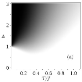
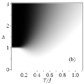
Figure 3: Density plot of concurrence $\mathcal{C}$ as function of $T/J$ and $\Delta$. Black color corresponds to the maximally entangled region, while by white color is the unentangled region, the gray region means the entanglement with degrees of different intensity. In (a) we display $\mathcal{C}$ for absence of the magnetic field and in (b) we display $\mathcal{C}$ for $h/J=1$.

In Fig. 3 we illustrate the density plot of concurrence $\mathcal{C}$ as a function of $T/J$ and $\Delta$ for a fixed value of $J_{1}/J$=1. Black corresponds to the maximum entangled region ($\mathcal{C}=1$), while white is the unentangled region ($\mathcal{C}=0$). Gray means the different degrees of entanglement ($0<\mathcal{C}<1$). After that we use this representation for the concurrence $\mathcal{C}$, depending on the parameters of the Hamiltonian (1). The entangled region represented by different gray intensities depends also on the temperature. For high temperature the fuzzy region increases, while for the low-temperature phase between the entangled region and the unentangled region the boundary becomes sharper. In Fig. 3(a) it is shown that the model is maximally entangled only for $\Delta\geqslant 1$ in the absence of the magnetic field, while the concurrence $\mathcal{C}$ is always less than 1 for $\Delta<1$ . The concurrence $\mathcal{C}$ becomes smaller with increasing temperature and the entanglement disappears at high temperatures. In Fig. 3(b) we display $\mathcal{C}$ for $h/J=1$, where the concurrence behaves similar to Fig. 3(a). But there is the maximum entangled region Fig. 3(b) for $\Delta\geqslant 1.0$ and at temperatures less than $T/J\thickapprox 0.2$.

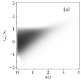
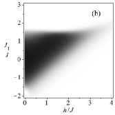
Figure 4: Density plot of concurrence $\mathcal{C}$ as function of $h/J$ and $J_{1}/J$ . In (a) we display of $\Delta=1.0$ and (b) is for $\Delta=2.0$. The black (white) region corresponds to $\mathcal{C}=1(0)$, and by gray regions we indicate a concurrence $0<\mathcal{C}<1$.

The density plot of concurrence $\mathcal{C}$ as a function of magnetic field $h/J$ and $J_{1}/J$ is shown in FIG.4 . To represent the concurrence we use the same representation as in Fig. 3, for a fixed value of $T/J=0.3$. In Fig. 4(a) we display $\mathcal{C}$ for a $\Delta=1.0$; thus, we can show that the concurrence is always less than $\mathcal{C}\lesssim 0.5$. The largest entanglement occurs for small $|J_{1}/J|\lesssim 1$ and small magnetic field $h/J\lesssim 2$. Whereas in Fig. 4(b) we display $\mathcal{C}$ for $\Delta=2.0$, and the entanglement becomes stronger than for $\Delta=1$, but the concurrence is still limited to the regions $|J_{1}/J|\lesssim 1.5$ and $h/J\lesssim 3$.

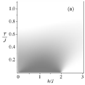
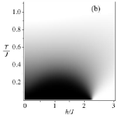
Figure 5: Density plot of concurrence $\mathcal{C}$ as a function of $h/J$ and $T/J$: In (a) we display $\mathcal{C}$ for a $\Delta=1$ and in (b) we display $\mathcal{C}$ for $\Delta=1.5$. The black (white) region corresponds to $\mathcal{C}=1(0)$, and by gray regions we indicate a concurrence $0<\mathcal{C}<1$.

Another case is shown in Fig. 5 for the density plot of concurrence $\mathcal{C}$ as a function of $h/J$ and $T/J$, at a fixed value of $J_{1}/J=1$. Black (white) region indicates the entangled (unentangled) region, while the gray region corresponds to $0<\mathcal{C}<1$. The concurrence is not very significant for $\Delta=1$, as shown in Fig. 5(a). For values of $0\leqslant h/J\lesssim 2$ the entanglement becomes $\mathcal{C}\lesssim 0.25$ at small temperatures, while at higher temperatures it disappears. For $\Delta=1.5$ the situation has changed; we observe the maximally entangled region for values of $0\leqslant h/J\lesssim 2.3$ and $T/J\lesssim 0.2$, as shown in Fig. 5 (b), and at higher temperatures and a strong magnetic field entanglement vanishes asymptotically.

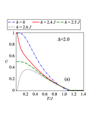
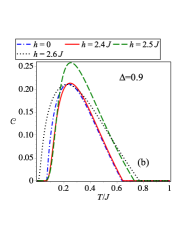
Figure 6: (Color online) Concurrence as a function of temperature for a fixed value of $J_{1}/J$=1: In (a) we displays concorrence for $\Delta=2$ and (b) displays concorrence for $\Delta=0.9$.

The concurrence as a function of temperature $T/J$ for fixed values of $J_{1}/J=1$ is shown in Fig. 6, for several values of the magnetic field. First of all, we illustrate the concurrence for $\Delta=2$ in Fig. 6(a). The concurrence reaches its maximum value $\mathcal{C}=1$ in the absence of magnetic field and at low temperature, whereas at high temperature entanglement disappears, the threshold temperature occurs at $T/J\approx 1.1$, which is represented by a dash-dotted line. The behavior of the concurrence varies in a strong magnetic field, and the entanglement curve in most cases is lower than in the absence of a magnetic field. In the case of $h/J=2.4$ (solid line), the maximum value of concurrence $\mathcal{C}=1$ is only achieved at very low temperature $T/J$, although the threshold temperature $T/J$ is slightly larger than that in the absence of a magnetic field. In the case of the magnetic field be $h/J=2.5$ (dashed line), the concurrence achieves the highest value around $\mathcal{C}=0.5$ at zero temperature. While for $h/J=2.6$ (dotted line), the system becomes unentangled at zero temperature, but at low temperatures near $T/J\thickapprox 0.3$ it reaches its maximum value around $\mathcal{C}\thickapprox 0.38$. Second, in Fig. 6(b) the behavior of the concurrence for a fixed value of the anisotropic parameter $\Delta=0.9$, and for different magnetic field values are shown. Now, the behavior of concurrence decreases with different values of the magnetic field and has a peak near $T/J\thickapprox 0.3$. The concurrence for all of these magnetic fields are unentangled at zero temperature and there is a temperature threshold near to $T_{th}/J\thickapprox 0.64$ for $0\leqslant h/J\lesssim 2.4$, while for $h/J\gtrsim 2.5$ the threshold temperature jumps to $T_{th}/J\gtrsim 0.75$.

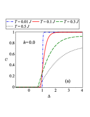
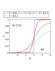
Figure 7: (Color online) Concurrence as a function of anisotropic parameter $\Delta$:(a) $h/J=0$ and (b) $h/J=2.5$ with different fixed values of temperature.

In Fig. 7(a) the concurrence as a function of the anisotropy parameter $\Delta$ in the absence of a magnetic field for various fixed temperatures is plotted. For $\Delta\lesssim 1$ the system is unentangled, and for $\Delta\gtrsim 1$ the system becomes entangled. The maximum of the entangled region is achieved for larger anisotropic parameters, but when the temperature increases the entanglement decreases. The concurrence as a function of the anisotropy parameter $\Delta$, and for a fixed magnetic field $h/J=2.5$ is plotted in Fig. 7(b), for the same set of temperatures as shown in Fig. 7(a). Here we can observe the influence of the magnetic field for the concurrence; at low temperature ($T/J=0.01$) the system is entangled for the values around of $\Delta\thickapprox 2$, whereas for higher temperature a small entanglement appears even for $\Delta<1$.

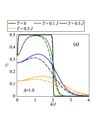
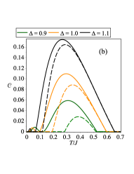
Figure 8: (Color online) (a) Concurrence against external magnetic field, for different values of temperature with anisotropic parameter $\Delta=1$. (b) Concurrence as a function of temperature assuming fixed values of the anisotropic parameter and a fixed magnetic field $hJ=0.2$. By the solid lines we represent the cluster-approach results ananikian whereas by the dashed lines we represent our result.

Finally, in Fig. 8(a) we display the concurrence as a function magnetic field, assuming a fixed value of the anisotropy parameter $\Delta=1$. In this plot the difference between the cluster approach ananikian and the transfer-matrix approach used here is also shown. By the solid lines we represent the transfer-matrix approach, while with dashed lines we denote the cluster approach ananikian . While, in Fig. 8(b) the concurrence as a function of temperature ($T/J$) is illustrated, by the continuous line we observe the cluster approach, and by the dashed line we represent our current result. For the anisotropic parameter $\Delta=1.1$ and for fixed magnetic field $h/J=0.2$. Clearly, the cluster approach shows a double peak (solid line), whereas by dashed lines we represent our current approach discussed here. Therefore, we can conclude that the small peak is absorbed due to the Ising coupling of the diamond chain structure. However, the small peak is rather irrelevant since the concurrence maximum value is around $\mathcal{C}\thickapprox 0.01$.

The difference between both approaches is consistent, since the entanglement on the diamond chain must be lower than for the cluster approach, where only the nearest Ising spins are considered, and we ignored the remaining diamond blocks coupling contributions, so the cluster approach is equivalent to infinite uncoupled diamond blocks.

IV.2 Entanglement threshold temperature

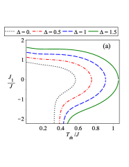
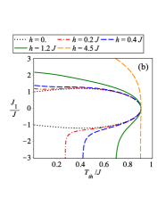
Figure 9: (Color online) Phase diagram, of Ising coupling parameter $J_{1}/J$ as a function threshold temperature $T_{th}/J$. (a) For several values of anisotropy parameter $\Delta$. (b) For several values of external magnetic field $h/J$.

In Fig. 9(a) we display the phase diagram of the entangled region and the untangled region, as a function of the Ising coupling parameter $J_{1}/J$ against threshold temperature for a fixed values of magnetic field $h/J=0.1$, and for several anisotropy parameters. For each curve the left side ($T/J<T_{th}/J)$ of this region corresponds to the entangled state, while for right side ($T/J>T_{th}/J$) the system becomes an unentangled region. The entangled region depends of the anisotropy parameter $\Delta$; as long as the anisotropy parameter increases the entangled region increases, too. For a large negative value of $J_{1}/J<0$, the unentangled region is limited around $T_{th}/J\gtrsim 0.3$, whereas, for $T_{th}/J\lesssim 0.3$ we still have an entangled region, although this entanglement leads to a weakly entangled region for large negative value of $J_{1}/J$, even for small a anisotropy parameter $\Delta$. However, for large positive value of $J_{1}/J$ the system becomes a fully unentangled region, but for large values of anisotropy parameter $\Delta$ tries to enhance the entanglement, although it always becomes an unentangled region for $J_{1}/J$ large enough. In Fig. 9(b) we display the phase diagram of entangled region and untangled region as a function of the Ising coupling parameter $J_{1}/J$ against threshold temperature for a fixed value of the anisotropy parameter $\Delta=1$, and for several values of magnetic field. For null magnetic field the entangled region is limited by the dotted curve, (the upper and lower side of this curve are symmetric), but as soon as the magnetic field is turned on, this symmetry is broken even for a low magnetic field like $h/J=0.2$ (described by the dash-dotted line), the system will always be entangled for $J_{1}/J\lesssim-1.5$ and $T_{th}/J\lesssim 0.28$. For a stronger magnetic field this limit increases until it achieves the asymptotic limit $T_{th}/J\approx 0.910239$. The largest value of threshold temperature $T_{th}/J\approx 0.910239$ occurs when $J_{1}/J=0$ and for arbitrary values of magnetic field. Of course, this limiting threshold temperature also depends on the magnitude of anisotropic parameters, as we can verify in Fig. 9(a).

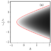
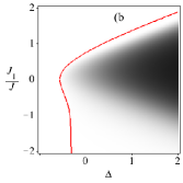
Figure 10: (Color online) Density plot concurrence $\mathcal{C}$ as function of $\Delta$ versus $J_{1}/J$. In (a) we display $\mathcal{C}$ for a null magnetic field and in (b), we display $\mathcal{C}$ $\mathcal{C}$ for $h/J=1$.

Other important density plots, are displayed in Fig. 10, for the concurrence $\mathcal{C}$ as a function of $\Delta$ against $J_{1}/J$, assuming a fixed temperature $T/J=0.3$. This density plots follow same pattern (definition) as those illustrated in Fig. 3; the black (white) region corresponds to $\mathcal{C}=1(0)$, while a gray region corresponds to $0<\mathcal{C}<1$. In Fig. 10(a) the maximally entangled region only appears for $\Delta>1$; we can also verify that the illustration is symmetric [($\mathcal{C}(J_{1}/J)=\mathcal{C}(-J_{1}/J))$] only when $h=0$. However, when the external magnetic field is turned on [i.e., ($h/J=1$)], the symmetry $J_{1}/J\leftrightarrow-J_{1}/J$ is broken as shown in Fig. 10(b). When $J_{1}/J>0$ the boundary between the entangled region and the unentangled region is sharper, while for $J_{1}/J<0$ the boundary between the entangled region and the unentangled region becomes less pronounced. The maximally entangled region becomes stronger for a large value of the anisotropy parameter $\Delta>1$ compared to the entanglement without magnetic field. This result is similar to the previous result discussed by Zhou et al. Zhou , when they studied the anisotropy effect of a two-qubit Heisenberg model with external magnetic field, although they discussed only one-couple qubits. The red solid line is used to represent the boundary between the entangled region and the unentangled region. This curve is also known as the threshold-temperature curve; clearly for null magnetic field the threshold temperature rounds symmetrically the entangled region-this is not so evident when external magnetic field is switched on. Even for a rather weak external magnetic field, the entangled region spreads out for $J_{1}/J<0$. The entanglement emerge for $J_{1}/J<-1$, [Fig. 10(b)], despite the concurrence being tiny and at first glance the concurrence still looks like in Fig. 10(a), but the threshold temperature is highly different compared to that without magnetic field, such as there is no threshold temperature for $J_{1}/J<-1$ and $\Delta\gtrsim-0.3$.

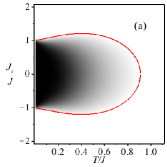
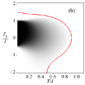
Figure 11: (Color online) Density plot concurrence $\mathcal{C}$ as function of $T/J$ versus $J_{1}/J$. In (a) we display $\mathcal{C}$ for a $h/J=0$ and in (b) we display $\mathcal{C}$ for $h/J=1$.

The density plot of concurrence $\mathcal{C}$ as a function of $T/J$ versus $J_{1}/J$ is depicted in Fig. 11, for a fixed value of $\Delta=1.0$. We show again that the maximally entangled region vanishes for higher temperature $T/J\approx 0.3$. In Fig. 11(a) the density plot of concurrence $\mathcal{C}$ is displayed for $h/J=0$, and the maximally entangled region is limited by $|J_{1}/J|\lesssim 1$, following the same kind of density plot as in Fig. 10, by the solid red line we represent the threshold temperature limiting the entangled region. Whereas for $h/J=1$, as displayed in Fig. 11(b), the maximally entangled region shrunk to $-0.5\lesssim J_{1}/J\lesssim 1$, despite the entangled region spread out with weakly entangled region for $J_{1}/J<0$ and $T_{d}/J\lesssim 0.5$, consequently the symmetry in $J_{1}/J\leftrightarrow-J_{1}/J$ is broken, this is better illustrated as a function of the threshold temperature curve described by the red solid line.

V Conclusions

In general most of the quantum entanglement studied of an infinite chain is a cumbersome issue, motivated by this fact we investigate the quantum entanglement of the Ising-XXZ diamond chain. Even when Ising coupling does not contribute directly in quantum entanglement, we discuss the Heisenberg two-qubit entanglement effect on Ising-Heisenberg diamond chain structure. First we obtain the Heisenberg dimer operators immersed in a diamond chain with Ising coupling. Using this result we are able to obtain the average of the two-qubit operator. Thereafter, the concurrence is obtained straightforwardly in terms of the reduced density matrix operator elements. Using the concurrence, we study the entanglement of the Ising-XXZ diamond chain as a function of Hamiltonian parameters, such as temperature as well as external magnetic field.

Usually the entangled region vanishes when the temperature increases; in some cases [see for instance Figs. 10(b) and 11(b)] the entanglement vanishes asymptotically when the external magnetic field is switched on. The entangled region is limited by the so-called threshold temperature, but for some other parameters [like in Figs. 10(b) and 11(b)] the threshold temperature only occurs in the asymptotic limit. From our result we conclude that there is no double peak in the concurrence as a function of temperature, such as that obtained by the use of the cluster approachananikian [see Fig. 8(b)]; the disappearance of the tiny peak can be understood as a dissipation due to the qubits are inmerse in diamond chain structure. However this small peak is irrelevant, since, the degree of entanglement is rather small: $\mathcal{C}=0.01$.

It would be interesting also in the future to consideration, the case of tripartite entanglement for Heisenberg coupling of an Ising-Heisenberg chain instead of bipartite Heisenberg coupling. Somewhat similar to that considered by Tsomokos et al. Tsomokos where the tripartite coupling was studied at the zero temperature.

References

- (1) L. Amico, R. Fazio, A. Osterloh and V. Vedral, Rev. Mod. Phys. 80, 517 (2008); R. Horodecki et al., Rev. Mod. Phys. 81, 865(2009); O. Gühne and G. Tóth, Phys. Rep. 474 1 (2009).
- (2) K. M. O’Connor and W. K. Wootters, Phys. Rev. A 63, 052302 (2001); Y. Sun, Y. Chen and H. Chen, Phys. Rev. A 68, 044301 (2003); G. L. Kamta and A. F. Starace, Phys. Rev. Lett. 88, 107901 (2002).
- (3) A. Honecker, S. Hu, R. Peters J. Ritcher, J. Phys.: Condens. Matter 23, 164211 (2011).
- (4) M. S. S. Pereira, F. A. B. F. de Moura, M. L. Lyra, Phys. Rev. B 77, 024402 (2008).
- (5) M. S. S. Pereira, F. A. B. F. de Moura, M. L. Lyra, Phys. Rev. B 79, 054427 (2009).
- (6) B. M. Lisnii, Low Temp. Phys. 37, 296 (2011).
- (7) L. Canova, J. Strečka, M. Jascur, J. Phys.: Condens. Matter 18, 4967 (2006).
- (8) O. Rojas, S.M. de Souza, V. Ohanyan, M. Khurshudyan, Phys. Rev. B 83 , 094430 (2011).
- (9) J.S. Valverde, O. Rojas, S.M. de Souza, J. Phys. Condens. Matter 20, 345208 (2008); O. Rojas, S.M. de Souza, Phys. Lett. A 375, 1295 (2011).
- (10) B. M. Lisnii, Ukrainian Journal of Physics 56, 1237 (2011).
- (11) K. C. Rule et al., Phys. Rev. Lett. 100, 117202 (2008).
- (12) H. Kikuchi et al., Phys. Rev. Lett. 94, 227201 (2005); H. Kikuchi et al., Prog. Theor. Phys. Suppl. 159, 1 (2005).
- (13) A. Honecker and A. Lauchli, Phys. Rev. B 63, 174407 (2001); B. Gu and G. Su, Phys. Rev. B 75, 174437 (2007); H. Jeschke et al., Phys. Rev. Lett. 106, 217201 (2011); J. Kang et al., J. Phys. Condens. Matter 21, 392201(2009); K Takano, K Kubo and H Sakamoto, J. Phys.: Condens. Matter 8, 6405 (1996); N. Ananikian, H. Lazaryan, and M. Nalbandyan, Eur. Phys. J. B 85, 223(2012); K Takano, K Kubo and H Sakamoto, J. Phys.: Condens. Matter 15, 5979 (2003).
- (14) F. Verstraete, M.A. Martin-Delgado, J.I. Cirac, Phys. Rev. Lett.92, 087201 (2004); M. Popp, F. Verstraete, M. A. Martin-Delgado, J. I. Cirac, Phys. Rev. A 71, 042306 (2005);
- (15) N. S. Ananikian, L. N. Ananikyan, L. A. Chakhmakhchyan and O. Rojas, J. Phys.: Condens. Matter 24, 256001 (2012).
- (16) L. Chakhmakhchyan, N. Ananikian, L. Ananikyan and C. Burdik, J. Phys: Conf. Series 343, 012022 (2012).
- (17) X. Wang, Phys. Rev. A 66, 044305 (2002).
- (18) Xiaoguang Wang, Phys. Rev. A 66, 034302 (2002)
- (19) M. C. Arnesen, S. Bose and V. Vedral, Phys. Rev. Lett. 87, 017901 (2001).
- (20) W. K. Wootters, Phys. Rev. Lett. 80, 2245 (1998).
- (21) S. Hill and W.K. Wootters, Phys. Rev. Lett. 78, 5022 (1997).
- (22) M. Fisher, Phys. Rev. 113, 969 (1959).
- (23) I. Syozi, Prog. Theor. Phys. 6, 341 (1951).
- (24) O. Rojas, J. S. Valverde, S. M. de Souza, Physica A 388, 1419 (2009); O. Rojas, S. M. de Souza, J. Phys. A: Math. Theor. 44, 245001 (2011).
- (25) J Strečka, Phys. Lett. A 374, 3718 (2010).
- (26) R.J. Baxter, Exactly Solved Models in Statistical Mechanics, (Academic Press, New York, 1982).
- (27) L. Zhou, H. S. Song, Y. Q. Guo and C. Li, Phys. Rev. A 68, 024301 (2003).
- (28) D. I. Tsomokos, J. J. Garcia-Ripoll, N. R. Cooper, and J. K. Pachos, Phys. Rev. A 77, 012106 (2008).