The Sub-Surface Structure of a Large Sample of Active Regions

Abstract

We employ ring-diagram analysis to study the sub-surface thermal structure of active regions. We present results using a large number of active regions over the course of Solar Cycle 23. We present both traditional inversions of ring-diagram frequency differences, with a total sample size of 264, and a statistical study using Principal Component Analysis. We confirm earlier results on smaller samples that sound speed and adiabatic index are changed below regions of strong magnetic field. We find that sound speed is decreased in the region between approximately $r=0.99\,R_{\odot}$ and $r=0.995\,R_{\odot}$ (depths of 3 Mm to 7 Mm), and increased in the region between $r=0.97\,R_{\odot}$ and $r=0.985R_{\odot}$ (depths of 11 Mm to 21 Mm). The adiabatic index [$\Gamma_{1}$] is enhanced in the same deeper layers that sound-speed enhancement is seen. A weak decrease in adiabatic index is seen in the shallower layers in many active regions. We find that the magnitudes of these perturbations depend on the strength of the surface magnetic field, but we find a great deal of scatter in this relation, implying other factors may be relevant.

1 Introduction

sec:intro Measurements of the thermal structure beneath active regions using the techniques of local helioseismology are of substantial interest in solar physics. An increasingly wide variety of sophisticated models of the structure of sunspots and active regions are becoming available, and helioseismology can be used to test the validity of these models. In this work, we use ring diagrams to study a large number of active regions from Solar Cycle 23.

The use of ring diagrams (Hill, 1988) to study the near-surface acoustic properties, dynamics, and thermal structure of the Sun is by now well established (e.g. review by Gizon and Birch, 2005). In previous works, inversions of ring-diagram frequencies for structure have been performed on small numbers of active regions (Basu, Antia, and Bogart, 2004; Bogart et al., 2008) to determine the changes in sound speed and adiabatic index. In these works, sound speed and adiabatic index were found to be enhanced in the layers between approximately $0.975\,R_{\odot}$ and $0.985\,R_{\odot}$, and depressed in the shallower layers between $0.99\,R_{\odot}$ and $0.998\,R_{\odot}$.

In this work, we study the sub-surface structure of a much larger sample of active regions than have previously been examined. We proceed in two ways: i) we simply extend the work of Basu, Antia, and Bogart (2004) and Bogart et al. (2008), performing structure inversions on ring-diagram data in the same manner as these earlier studies, and ii) in order to better take advantage of the large data set that we have, we perform a Principal Component Analysis (PCA) and study the resulting principal components. In Section sec:data we introduce the ring-diagram data sets that we use in this work and discuss the differences between the sample that we use for individual inversions and the sample that we use in our PCA. In Section sec:pca, we describe the use of Principal Component Analysis to study the ring-diagram mode parameters. In Section sec:inv, we present the inversions of both a large number of individual rings and of the principal components from Section sec:pca. We summarize our findings in Section sec:conc.

2 Data

sec:data

2.1 Ring Diagrams

Ring diagrams are three-dimensional power spectra of localized regions on the Sun. In this work, the data are resolved line-of-sight Doppler measurements (“Dopplergrams”) taken with the Michelson Doppler Imager (MDI) instrument on the Solar and Heliospheric Observatory (SOHO). In order to achieve sufficiently high spatial frequency and sufficient signal-to-noise, we use only full-disk Dopplergrams, and require a duty cycle greater than 80%. Because full-disk data are an MDI high-rate data product, sufficient data coverage is only available during yearly Dynamics campaigns, which are typically two or three months long. The data have a one-minute cadence and are tracked for 8192 minutes. The midpoint of the tracking interval coincides with the region of interest crossing the central meridian of the solar disk. The data are projected onto a rectangular grid using Postel’s projection and corrected for the distortion in the MDI optics. This process is described in more detail by Patron et al. (1997) and Basu, Antia, and Tripathy (1999).

The spectra are fit in the way described by Basu, Antia, and Bogart (2004). A model of the power spectrum with 13 free parameters is fit at constant frequency. This model accounts for advection in the zonal and meridional directions as well as asymmetry in the spatial frequency direction and azimuthally around the ring. The parameter of interest in this work is the spatial frequency [$k$], which is returned as a function of the temporal frequency [$\nu$] and the radial order [$n$]. In the plane-wave approximation the spatial frequency is related to the spherical harmonic degree [$\ell$] by $\ell=kR_{\odot}$. We interpolate the ring fits to integer values of $\ell$ and interpret them in the same way as global mode parameters. We will refer to these interpolated ring-diagram fits as “mode parameter sets”; all results in this work are based on these data sets.

The level of activity in a ring is characterized by a Magnetic Activity Index (MAI: Basu, Antia, and Bogart, 2004). This is a measure of the strong unsigned magnetic flux within the ring-diagram aperture, averaged over the tracking period.

2.2 Ring Diagram Selection

In this work, we use two different data sets to study the structure beneath active regions. The first set consists of a set of frequency differences between active regions from the NOAA catalog and nearby regions of quiet Sun, and is essentially equivalent to the data sets used in earlier works (e.g. Basu, Antia, and Tripathy, 1999; Rajaguru, Basu, and Antia, 2001; Basu, Antia, and Bogart, 2004), albeit with a much larger sample. The second set consists of mode frequencies for a set of largely non-overlapping rings, and is used for the statistical study described in Section sec:pca.

The first sample is the same sample used by Baldner, Bogart, and Basu (2011a). Regions are selected from the NOAA active-region catalog between June 1996 and April 2008. We include only NOAA active regions that are identified at disk center — in other words, we require that the active region be present through the center of the tracking interval. We require, too, sufficient data coverage as noted above. As in Basu, Antia, and Bogart (2004), we perform inversions relative to quiet-Sun ring-diagram mode parameters. The comparison ring diagrams are tracked at the same latitude as the active region that they are compared with. They are tracked across the disk in exactly the same way as the active regions, and are located within 60^∘ longitude of their active region. This is done to minimize the systematic errors in mode-parameter estimation arising from projection effects and secular changes in the instrument, as well as to minimize the effects of difficulties in modeling the near-surface layers of the solar interior. A preliminary version of this analysis was presented by Baldner, Bogart, and Basu (2011b). Although the parent active-region sample is the same in both works, the actual ring-diagram data used in the inversions have changed somewhat — in particular, the mode sets used and the comparison regions chosen. The most significant changes to the data set are improved treatment of the errors in the mode fitting and inversion, and more careful comparison region selection.

The second data set in this work is used in the PCA described in the next section. We use mode frequencies rather than frequency differences for the PCA itself. The PCA requires a filled matrix of mode parameters [$\nu_{n,\ell}$] for a set of modes common to all of the rings in the sample. A common set of [$n,\ell$] modes are chosen, and the ring-diagram fits are interpolated to these targets.

For the PCA procedure, we wish to minimize overlapping data, which could lead to some spurious statistical results. We choose only ring diagrams that were constructed from tracked data patches that do not overlap. The ring diagrams in this sample are the same size and tracking length as in the data set used for our individual inversions but are distributed somewhat differently so as to minimize spatial overlap rather than guaranteeing coverage of all NOAA active regions.

3 Principal Component Analysis

sec:pca The use of Principal Component Analysis (PCA) in the analysis of helioseismic data was described by Baldner and Basu (2008) in the context of global-mode analysis. In brief, PCA finds an efficient representation of a set of data vectors as a linear combination of orthogonal principal components. It is efficient in the sense that, when properly ordered, each principal component is responsible for less variance in the data than the one that precedes it. In many applications, the data can be adequately represented using a relatively small number of principal components. An added benefit is that errors in measurements can be greatly reduced. In this work, we are primarily interested in using PCA to separate spurious signals in the mode parameters from those actually associated with solar activity, and to parametrize the changes in solar structure around active regions in a simple manner.

We use the following notation: if the set of all $m$ frequency measurements $\nu_{j}$ for the $i$th ring diagram form the vector $\mathbf{D}_{i}=\{\nu_{0}\ldots\nu_{m}\}$, each observation $\mathbf{D}_{i}$ can be reproduced completely with the $m$ principal components $\xi_{k}$ (each a vector of length $m$) and the $m$ scaling coefficients $c_{k,i}$ associated with that measurement:

$$\mathbf{D}_{i}=\sum_{k=0}^{m}c_{k,i}\xi_{k}.$$ (1)

The principal components [$\xi_{k}$] are normalized to unity. Errors in each component of the principal components and in the scaling coefficients are computed using a Monte Carlo simulation.

The results of the PCA are shown in Figure fig:pcavec. The first component may be interpreted as the basic $\ell$ – $\nu$ diagram for a ring-diagram fit. The scaling coefficients [$c_{1}$] give the appropriate scaling for each observation, and we can see a general trend with increasing magnetic activity, although the scatter is large. The second component also has a significant dependence on magnetic activity. The following two principal components which are shown in Figure fig:pcavec and are dominated by tails at the end of each $n$ ridge. These tails arise in the fits as the signal-to-noise decreases at the high-$\ell$ end of a ridge or the ridges begin to overlap significantly at low $\ell$. In either case, the fits become less reliable. In inversions on real data, we truncate the fits as these tails become significant.

Higher-order components are not shown — they are in general dominated either by tails or by small numbers of outliers. Most of these components are significant only in one or at most a small number of rings. Some components show dependence on latitude (for example, $\xi_{5}$ and $\xi_{12}$) or on epoch ($\xi_{7}$). By choosing to neglect these components when reconstructing the data sets, we remove many small systematic effects and errors from the frequency measurements.

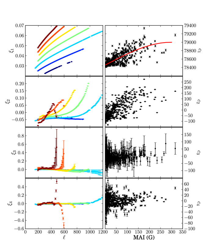
Figure 1.: The first four principal components and the associated scaling coefficients. The first four principal components ($\xi_{1}$ through $\xi_{4}$) are shown in the left-hand panels as a function of degree [$\ell$]. Each order [$n$] is shown in a different color. The right-hand panels show the scaling coefficients for each ring as a function of the ring’s MAI. The red line in the top-right panel is a smoothed fit to the scaling coefficients.fig:pcavec

Given the apparent dependence of the scaling coefficients $c_{1}$ and $c_{2}$ on magnetic activity, it is desirable to reduce these coefficients to simple functions of MAI. In Figure fig:pcavec, we show a smoothed fit using B-splines to the $c_{1}$ coefficients as a function of MAI. These may be used to approximate the dependence of these coefficients on magnetic activity. Since $c_{1}$ and $c_{2}$ both depend on MAI, we examine in Figure fig:coef their dependence on each other. It is clear that they are tightly correlated. Thus, for a given $c_{1}$, which we can relate approximately to MAI, we can determine $c_{2}$ fairly accurately. The scaling coefficients $c_{3}$ for the third principal component do not correlate well with $c_{1}$ or $c_{2}$, or with any other quantity that we examined.

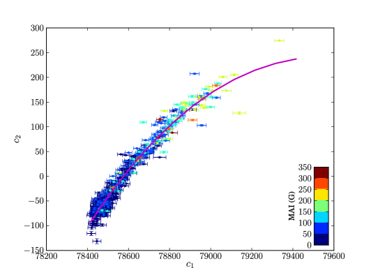
Figure 2.: The second principal component scaling coefficients as a function of the first. The points are color-coded by MAI. The magenta line is a smoothed B-spline fit to the points.fig:coef

It is important to know how well we can reproduce the actual ring-diagram mode parameters with a small number of vectors. In Figure fig:resid we plot the residuals between the reconstruction using three principal components of three randomly selected rings, and the actual ring data. We find that, especially for low MAIs, the agreement is fairly good. At the edges of ridges there are discrepancies, but as noted above, the spectrum fits tend to become unreliable at either end of the power ridges.

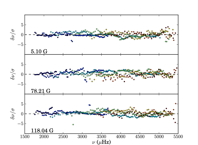
Figure 3.: The difference between frequencies obtained from three ring diagrams and their representations using the first two principal components. The residuals are divided by their errors. The MAIs of the three rings are shown in the lower right. As in Figure fig:pcavec, different orders $n$ are plotted in different colors.fig:resid

4 Inversions for Structure

sec:inv To determine the structure of the solar layers beneath active regions (or, in general, regions of high surface magnetic field), we invert frequency differences for sound speed or for the first adiabatic index [$\Gamma_{1}$]. The treatment of this problem as a linear inversion is by now well established both in global and in local seismology. In this work, we use Subtractive Optimally Localized Averages (SOLA: Pijpers and Thompson, 1992, 1994) to perform the inversions.

In our SOLA inversion, there are four free parameters: the error suppression parameter ($\mu$), the cross-term trade-off parameter [$\beta$], the width of the target kernel [$\Delta_{A}$], and the number of B-splines used to remove the surface term [$\Lambda$]. The selection of these parameters has been described in earlier works, e.g. Rabello-Soares, Basu, and Christensen-Dalsgaard (1999).

4.1 Inversions of Individual Rings

The principal difficulty in performing an inversion for structure from helioseismic data is in choosing the appropriate inversion parameters, which has limited earlier works. Baldner, Bogart, and Basu (2011b) found that a few combinations of inversion parameters worked well on a small subset of the active regions in our sample that was studied in detail. In this work, we again performed a thorough exploration of the parameter space on a small subset of the rings, including comparisons to rings published in earlier works. We find that the inversion results are not strongly dependent on the choice of surface term, so long as a surface term is used. When the surface term is not included in the inversions, very large perturbations are returned by the perturbations which are almost certainly spurious. We restrict ourselves to $\Lambda=4$. In exploring the effects of the target kernel width, we find smaller values of $\Delta(r_{0})$ tend to cause oscillatory solutions to many inversions. Since we have not found any particularly sharp features in our inversions, we use a fairly large value of $\Delta(r_{0})=0.055$, which suppresses some oscillatory behavior in certain inversions, and does not overly smooth actual structure in better inversions.

Finally, for the choices of the error suppression term and the trade-off parameter, we have found that the values of these parameters for acceptable inversions in the rings we have examined carefully fall in a fairly narrow range. For the full sample, then, we run a batch of inversions for each region over the sample. Examining the inversions for each region can then be done fairly quickly and the best set of inversion parameters selected. We reject regions with unstable inversions — that is, regions whose inversion results are very strongly dependent on the choice of inversion parameters. What remains comprises our sample of sound speed and adiabatic index inversions.

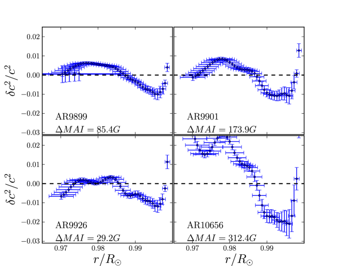
Figure 4.: Examples of inversions for adiabatic squared sound speed [$c^{2}$] for four active regions. The sense of the inversions is active minus quiet. The plotted horizontal error bars are the distance between the first and third quartile points of the inversion averaging kernels, and represent the resolution of the inversion. The vertical error bars are the formal errors in the inversions.fig:c2ex

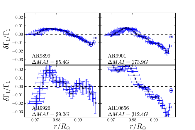
Figure 5.: Examples of inversions for adiabatic index [$\Gamma_{1}$] for four active regions. The regions shown are the same as those in Figure fig:c2ex.fig:g1ex

Inversions for the difference in squared sound speed [$c^{2}$] and adiabatic index [$\Gamma_{1}$] were performed for all regions in the sample with $\Delta$ MAI $>$ 40 G. Figure fig:c2ex shows example sound-speed inversions for four different rings with a range of active-region strengths as a function of depth. Figure fig:g1ex shows inversions for adiabatic index for the same regions.

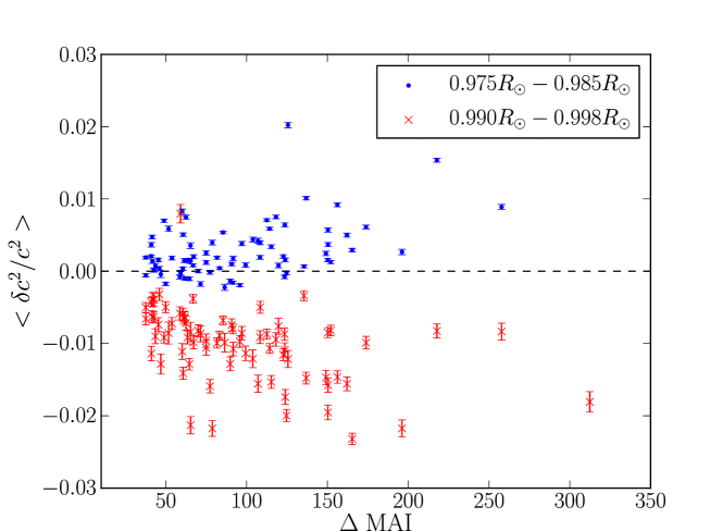
Figure 6.: Averages of inversions for $c^{2}$ over two depth ranges are shown, plotted as a function of $\Delta$ MAI. Blue points are averages of inverted sound speed between $0.975\,R_{\odot}$ and $0.985\,R_{\odot}$; red crosses are averages of inverted sound-speed difference between $0.99\,R_{\odot}$ and $0.998\,R_{\odot}$.fig:c2

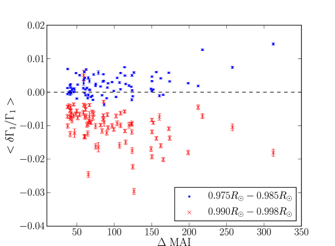
Figure 7.: Averages of inversions for differences in $\Gamma_{1}$ over two depth ranges are shown, plotted as a function of $\Delta$ MAI. Blue points are averages of inverted sound speed between $0.975\,R_{\odot}$ and $0.985\,R_{\odot}$; red crosses are averages of inverted sound speed between $0.99\,R_{\odot}$ and $0.998\,R_{\odot}$.fig:g1

Figure fig:c2 shows averages of the inverted sound speed for all regions in our sample for different depth ranges. For sound speed averaged between $0.975R_{\odot}$ and $0.985R_{\odot}$, sound speeds are generally enhanced in the presence of magnetic fields, while in the region from $0.99R_{\odot}$ to $0.998R_{\odot}$, sound speeds decrease. In both regions, the magnitude of the change tends to increase with magnetic-field strength, although the relationship seems to be more of an envelope than a linear relation. Further, there seems to be some saturation of the effect at very high magnetic-field strengths.

In the shallowest layers ($r>0.998\,R_{\odot}$), the sound-speed inversion results show a sharp positive change. This feature is present in every inversion in our sample. Caution should be used in interpreting this, however, as the averaging kernels become strongly asymmetric near the surface and the cross-term contributions begin to become significant. Examples of this sharp feature can be seen in the inversions in Figure fig:c2ex.

We have also inverted for the first adiabatic index. In Figure fig:g1, we show the same averages as Figure fig:c2, but for the $\Gamma_{1}$ inversions. In general, $\Gamma_{1}$ is an easier quantity to invert for (in the sense that the inversions tend to be less sensitive to the inversion parameters), and so we include a larger number of inversions for $\Gamma_{1}$ than we could for $c^{2}$.

We find that, as for the $c^{2}$ results, there is a depression in $\Gamma_{1}$ in the shallower layers that we invert (above $r=0.99\,R_{\odot}$), and that, in many cases, there is a corresponding enhancement below approximately $r=0.98\,R_{\odot}$, as was found in earlier works. We find that the deeper enhancement is, for most rings, much less pronounced than for the $c^{2}$. For some regions, in fact, we do not see any positive perturbation at all, and in general we find only a weak correlation with magnetic activity.

The depth ranges of the negative and positive perturbations are found to be relatively constant. In Figure fig:crossc2, we plot the depths at which our inversion results change from negative to positive. We find that, at lower activity levels, there is greater variance in the depths of the perturbations, but this can be explained by lower signal-to-noise in the inversions. Beyond that, we do not find any significant change in the depth ranges of the perturbations.

  

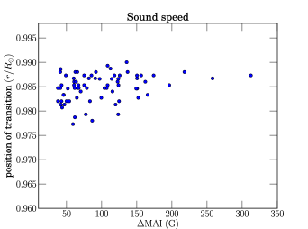
Figure 8.: Position of transition, in fractional radius, between the negative (shallower) inversion results and the deeper (positive) perturbations in the inversion results, plotted as a function of $\Delta$ MAI. At left, the sound speed results are shown, at right are the results for adiabatic index. These transition points are found by treating the inversion points as a continuous curve and finding the zero-crossing point.fig:crossc2

4.2 Inversions of PCA Data

sec:invpca In this section we use the PCA reconstruction of ring-diagram mode parameters described in Section sec:pca to perform inversions for structure. As discussed earlier, the advantages of using PCA on this data set are reduced errors in the reconstructed data set and removal of certain systematic effects in parameter estimation due to secular changes in the MDI instrument over time and projection effects. In addition, because we may reduce the data to a number of linearly independent vectors, we substantially reduce the number of inversions that need to be done.

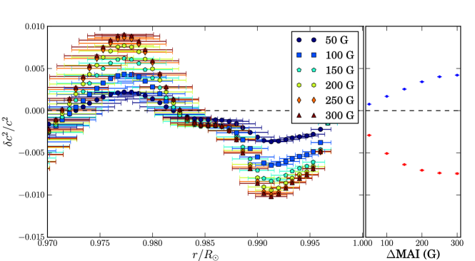
Figure 9.: Inversion of the first two principal components at different MAIs for $c^{2}$. The scaling coefficients are chosen as discussed in the text. The left-hand panel shows individual inversions as a function of radius. As in Figure fig:c2ex, the horizontal error bars are the difference between the first and third quartile points of the averaging kernels, and represent the resolution of the inversion. The vertical error bars are the formal errors in the inverted quantities. The latter are generally smaller than the points. The right-hand panel shows the average of the inversion results over the same depth ranges as Figure fig:c2 as a function of MAI.fig:pcacsq

Most of the variation in the ring-diagram mode parameter sets are spanned by the first two principal components (see Figure fig:resid). Furthermore, as the coefficients $c_{1}$ are relatively well correlated with MAI, and $c_{2}$ is tightly correlated with $c_{1}$, we can reconstruct ring-diagram frequencies as a function of MAI. We then compute frequencies [$\nu_{n,\ell}$], the difference in frequency [$\delta\nu_{n,\ell}$] between the target MAI and zero MAI, and the error in $\delta\nu_{n,\ell}$. With these quantities, we may perform a SOLA inversion in the same manner as in the previous section.

The inversion results for six target MAIs between 50 G and 300 G are shown in Figure fig:pcacsq. As in the inversions of individual rings, the inversions of the PCA reconstructions show a distinctive two-layer structure with a shallow negative perturbation and a deeper positive perturbation. In addition, the magnitudes of these perturbations scale with MAI, and the saturation effect hinted at in the results in Figure fig:c2 is clearly present here.

While most of the variation is spanned by $\xi_{1}$ and $\xi_{2}$, there remains significant signal in subsequent components. We are interested to know, then, what effects these higher components have on inversions for structure, and so we invert components separately. It must be noted, however, that inversion results from different components, each with different errors, cannot be simply combined together linearly. With that in mind, we proceed to invert various principal components separately.

In Figure fig:vecinv, we show inversions for sound speed for principal components $\xi_{2}$ through $\xi_{5}$. Because it is not clear how to parametrize the scaling coefficients for any of the components except $\xi_{2}$, we simply scale the component by the largest coefficient for that component, and perform the inversion. We invert the components themselves, not explicit differences — thus the inverted sound speeds are the difference between a ring with a large coefficient $c_{i}$ and a ring without any contribution from that component at all. We see that $\xi_{3}$ and $\xi_{4}$ do return changes in structure, but $\xi_{5}$ is consistent with no change.

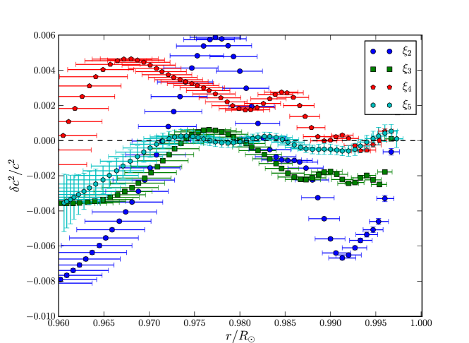
Figure 10.: Inversion of the $\xi_{2}$ through $\xi_{5}$ principal components individually. Each component $\xi_{i}$ is scaled by the largest associated coefficient $c_{i}$ in our data set. The base frequencies are the same as the base frequencies used in Figure fig:pcacsq.fig:vecinv

We also invert for adiabatic index. Figure fig:pcag1 shows inversions for the first two principal components at various MAIs between 50 G and 300 G. We find general consistency with the individual ring-diagram inversions: a shallow negative and deeper positive perturbation. The correlation with MAI in the shallow layer is very weak, and in some rings there is no negative perturbation at all. We find that the boundary between the negative and positive perturbations is somewhat deeper than in the individual inversion for $\Gamma_{1}$, occurring between $0.975\,R_{\odot}$ and $0.98\,R_{\odot}$. This discrepancy does not appear to arise from the choice of modes used in the inversion, nor does it depend on the choice of inversion parameters. One possibility is that the contributions from other principal components may shift the boundary upward, which would in turn imply a dependence of $\Gamma_{1}$ on something other than MAI. This is in fact what we find. On examination, the $\xi_{4}$ principal component returns a positive perturbation in the region we expect, and little signal elsewhere. The magnitude of the $\xi_{4}$ component (the $c_{4}$ coefficients from Figure fig:pcavec) show a large scatter at low MAI values, but a pronounced bump above approximately 150G. This is broadly consistent with the individual inversion results shown in Figure fig:g1, where many of the regions with $\Delta$ MAI $<$ 150G do not show positive perturbations.

We have explored the first ten principal components in some detail and not found evidence of this, however.

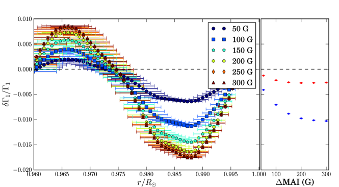
Figure 11.: Inversion of the first two principal components at different MAIs for adiabatic index [$\Gamma_{1}$]. The data are the same as those inverted in Figure fig:pcacsq. The left hand panel shows the individual inversions, the right hand panel shows averages over the same depth ranges as Figure fig:g1 as a function of MAI.fig:pcag1

5 Conclusions

sec:conc In this work, we have presented inversions for structure of a large number of active regions, and used Principal Component Analysis to parametrize more accurately these inversion results. We confirm earlier results using ring-diagram analysis (Basu, Antia, and Bogart, 2004; Bogart et al., 2008), as well as high-degree global-mode analysis (Rabello-Soares, 2012) that finds a two-layer thermal structure beneath surface magnetic activity. We find a shallow negative sound speed perturbation and a somewhat deeper positive perturbation, with a similar structure in the adiabatic index. The magnitudes of these perturbations generally increase with the magnitude of the surface magnetic field.

Bogart et al. (2008) found a linear correlation between magnitude of the sound-speed change and strength of the active region. We find a similar relation, but with substantial scatter in our inversions of individual rings. It is perhaps more correct to say that we find an “envelope” related to MAI than a real correlation. Further, we find that the correlation appears to saturate at high field strengths. We find that the positive perturbation in $\Gamma_{1}$ is much weaker than in $c^{2}$, and that the correlation with magnetic activity is much less significant. We find consistent values for the strength of the perturbations in the shallower layers with Basu, Antia, and Bogart (2004) and with Bogart et al. (2008), but we find consistently smaller values for the deeper, positive perturbations than those found in the previous works. The choices of inversion parameters and mode sets can have some effect on the magnitudes of the inversions. In Basu, Antia, and Bogart (2004), RLS inversions tended to return slightly larger perturbations than the SOLA inversions, which we employ in this work. The most significant effect on our results appears to be our decision to neglect the $f$-mode in our inversions, which, as noted above, made our inversion results more stable. It also appears to have decreased the magnitude of the sound-speed change in the deeper layers.

Bogart et al. (2008) also reported that the depths of the positive perturbations in $\Gamma_{1}$ were deeper than those in the $c^{2}$ inversions. We find this unambiguously in the PCA inversion results (Figure fig:pcag1), and it is also consistent with the inversions of individual rings.

Interpreting these results is not straightforward. The inversions that we perform in this work are, strictly speaking, only valid in a spherically symmetric, non-magnetized star. Clearly, neither of these conditions is satisfied in active regions. In the presence of magnetic fields, wave propagation is affected both by the direct effect of the Lorentz force, and by the effects of magnetic fields on the thermal structure. At some point — at some minimum field strength or field configuration — the entire linearized inversion becomes meaningless, as the contributions from magnetic fields to the wave propagation (which is, among other problems, no longer insensitive to direction) become significant.

In some studies, the choice is made to interpret the inferred change in sound speed as a change in the local wave speed, as was done in Gizon et al. (2009) and Moradi et al. (2010), rather than interpreting it as the effects of a thermal perturbation as we do here. In these works, significant disagreement was found when ring-diagram inversions were compared to time–distance inversions for the same solar data. The resolution of this discrepancy remains unclear. If we do in fact measure a wave speed perturbation in this work, Lin, Basu, and Li (2009) have claimed that the magnetic effect can be disentangled from the thermal effect. In the case of time–distance analysis, Braun et al. (2012) have shown that travel-time shifts determined from a model sunspot match neither what the thermal perturbation should give nor what they would expect from the magnetoacoustic fast mode speed. The implication of this work is that, in the case of time–distance analysis, at least, it is not correct to interpret inversion results as either changes in the thermal sound speed or as local wave speed perturbations. Equivalent work has not yet been done for ring-diagram analysis, but must be done to determine the extent to which the assumptions we have made are valid.

In studying our sample of rings using PCA, we have decomposed the ring diagram frequency measurements into a set of linearly independent components. The dependence of the first two of these on magnetic activity allows us to parametrize most of the frequency variance across our sample of rings as a function of MAI, and to determine what changes in sound speed and adiabatic index could give rise to these changes. We find that both sound speed and adiabatic index have a dependence on MAI that is consistent with what has been found in individual rings.

There is further variance in the ring-diagram frequency measurements, however, and MAI alone does not adequately parametrize the ring-diagram frequencies, as can be seen in Figure fig:pcavec. Many of these changes are due to errors in the ring fitting and systematic effects due to projection effects and secular changes in the MDI instrument, but some of the more significant principal components may represent changes that are solar in origin and that may be associated with thermal changes below the solar surface, as shown in Figure fig:vecinv.

We have demonstrated that PCA can be a useful tool in ring-diagram analysis and structure inversion. The large volume of data being returned from the Helioseismic and Magnetic Imager (HMI) on the Solar Dynamics Observatory (SDO) spacecraft represents a significant data analysis challenge — it is possible that this technique might prove a feasible alternative to attempting inversions on every ring diagram produced by HMI.

Acknowledgements

This work was partially supported by a NASA Earth and Space Sciences fellowship NNX08AY41H to CSB. CSB and RSB are currently supported by NASA grant NAS5-02139 to Stanford University. SB acknowledges support from NASA grant NNX10AE60G. This work utilizes data from the Solar Oscillations Investigation/Michelson Doppler Imager (SOI/MDI) on the Solar and Heliospheric Observatory (SOHO). SOHO is a project of international cooperation between ESA and NASA. MDI is supported by NASA grant NNX09AI90G to Stanford University.

References

- Baldner and Basu (2008) Baldner, C.S., Basu, S.: 2008, Solar Cycle Related Changes at the Base of the Convection Zone. ApJ 686, 1349 – 1361. doi:10.1086/591514.
- Baldner, Bogart, and Basu (2011a) Baldner, C.S., Bogart, R.S., Basu, S.: 2011a, Evidence for Solar Frequency Dependence on Sunspot Type. ApJ 733, 5. doi:10.1088/2041-8205/733/1/L5.
- Baldner, Bogart, and Basu (2011b) Baldner, C.S., Bogart, R.S., Basu, S.: 2011b, The thermal structure of sunspots from ring diagram analysis. J. Phys. Conf. Ser. 271(1), 012006. doi:10.1088/1742-6596/271/1/012006.
- Basu, Antia, and Bogart (2004) Basu, S., Antia, H.M., Bogart, R.S.: 2004, Ring-Diagram Analysis of the Structure of Solar Active Regions. ApJ 610, 1157 – 1168. doi:10.1086/421843.
- Basu, Antia, and Tripathy (1999) Basu, S., Antia, H.M., Tripathy, S.C.: 1999, Ring Diagram Analysis of Near-Surface Flows in the Sun. ApJ 512, 458 – 470. doi:10.1086/306765.
- Bogart et al. (2008) Bogart, R.S., Basu, S., Rabello-Soares, M.C., Antia, H.M.: 2008, Probing the Subsurface Structures of Active Regions with Ring-Diagram Analysis. Sol. Phys. 251, 439 – 451. doi:10.1007/s11207-008-9213-9.
- Braun et al. (2012) Braun, D.C., Birch, A.C., Rempel, M., Duvall, T.L.: 2012, Helioseismology of a Realistic Magnetoconvective Sunspot Simulation. ApJ 744, 77. doi:10.1088/0004-637X/744/1/77.
- Gizon and Birch (2005) Gizon, L., Birch, A.C.: 2005, Local Helioseismology. Living Reviews in Solar Physics 2, No.1 (http://www.livingreviews.org/lrsp-2005-6)
- Gizon et al. (2009) Gizon, L., Schunker, H., Baldner, C.S., Basu, S., Birch, A.C., Bogart, R.S., Braun, D.C., Cameron, R., Duvall, T.L., Hanasoge, S.M., Jackiewicz, J., Roth, M., Stahn, T., Thompson, M.J., Zharkov, S.: 2009, Helioseismology of Sunspots: A Case Study of NOAA Region 9787. Space Sci. Rev. 144, 249 – 273. doi:10.1007/s11214-008-9466-5.
- Hill (1988) Hill, F.: 1988, Rings and trumpets - Three-dimensional power spectra of solar oscillations. ApJ 333, 996 – 1013. doi:10.1086/166807.
- Lin, Basu, and Li (2009) Lin, C.-H., Basu, S., Li, L.: 2009, Interpreting Helioseismic Structure Inversion Results of Solar Active Regions. Sol. Phys. 257, 37 – 60. doi:10.1007/s11207-009-9332-y.
- Moradi et al. (2010) Moradi, H., Baldner, C., Birch, A.C., Braun, D.C., Cameron, R.H., Duvall, T.L., Gizon, L., Haber, D., Hanasoge, S.M., Hindman, B.W., Jackiewicz, J., Khomenko, E., Komm, R., Rajaguru, P., Rempel, M., Roth, M., Schlichenmaier, R., Schunker, H., Spruit, H.C., Strassmeier, K.G., Thompson, M.J., Zharkov, S.: 2010, Modeling the Subsurface Structure of Sunspots. Sol. Phys. 267, 1 – 62. doi:10.1007/s11207-010-9630-4.
- Patron et al. (1997) Patron, J., Gonzalez Hernandez, I., Chou, D.-Y., Sun, M.-T., Mu, T.-M., Loudagh, S., Bala, B., Chou, Y.-P., Lin, C.-H., Huang, I.-J., Jimenez, A., Rabello-Soares, M.C., Ai, G., Wang, G.-P., Zirin, H., Marquette, W., Nenow, J., Ehgamberdiev, S., Khalikov, S., TON Team: 1997, Comparison of Two Fitting Methods for Ring Diagram Analysis of Very High L Solar Oscillations. ApJ 485, 869. doi:10.1086/304469.
- Pijpers and Thompson (1992) Pijpers, F.P., Thompson, M.J.: 1992, Faster formulations of the optimally localized averages method for helioseismic inversions. A&A 262, L33 – L36.
- Pijpers and Thompson (1994) Pijpers, F.P., Thompson, M.J.: 1994, The SOLA method for helioseismic inversion. A&A 281, 231 – 240.
- Rabello-Soares (2012) Rabello-Soares, M.C.: 2012, Solar-cycle Variation of Sound Speed near the Solar Surface. ApJ 745, 184. doi:10.1088/0004-637X/745/2/184.
- Rabello-Soares, Basu, and Christensen-Dalsgaard (1999) Rabello-Soares, M.C., Basu, S., Christensen-Dalsgaard, J.: 1999, On the choice of parameters in solar-structure inversion. MNRAS 309, 35 – 47. doi:10.1046/j.1365-8711.1999.02785.x.
- Rajaguru, Basu, and Antia (2001) Rajaguru, S.P., Basu, S., Antia, H.M.: 2001, Ring Diagram Analysis of the Characteristics of Solar Oscillation Modes in Active Regions. ApJ 563, 410 – 418. doi:10.1086/323780.