A Yang-Mills Type Gauge Theory of Gravity and the Dark Matter and Dark Energy Problems

Abstract

A Yang-Mills type gauge theory of gravity is shown to have a structure richer than that of the Einstein’s General Theory of Relativity. This new structure can give an explanation of the form of the galactic rotation curves, of the amount of intergalactic gravitational lensing, and of the accelerating expansion of the Universe.

1 Introduction

In the past decades, many new discoveries in astronomy that might have something to do with gravity are coming in. For example, stellar objects at the spiral arms of galaxies are rotating at faster speeds than that can be explained by the Keplerian motions. To overcome this difficulty, people assume that some extra matter, not visible to us, is giving an extra pull on these stellar objects. Extra light deflections, as observed in the intergalactic gravitational lensing, are also ascribed to the existence of this extra matter. This is as known as the Dark Matter problem. An equally well known fact is that the Universe is accelerating in its expansion. This is in contrast to our expectation that the Universe should be decelerating, unless some extra energy is kept pumping into the Universe. This is the so called the Dark Energy problem

The expected Keplerian motions of stellar objects in the galactic spiral arms and the expected decelerating expansion of the Universe are something that are predicted by solving the Einstein Field Equation of General Relativity under the visibly observed mass-energy distributions in the spiral galaxies and in the Universe. The deviations from these expectations are attributed to, by most people, the existence of dark matter and dark energy. But it could well happen that the General Theory of Relativity is not sophisticated enough to explain all these observed phenomena in gravity. Here we are taking this point of view, and are proceeding to see if we can obtain an explanation of these anomalous astronomical phenomena by going beyond Einstein’s General Theory of Relativity.

2 A Yang-Mills type gauge theory of gravity

There, by now, exist many modifications to Einstein’s General Theory of Relativity so as to tackle gravity. Given the great success of the Yang-Mills way of describing the electroweak and the strong interactions, we believe that the Yang-Mills way could also be a good approach to describe the gravitational interaction.

The Yang-Mills type of action that describes gravitation will be taken to be the form of

$${\rm S_{YM}}\left[g,\Gamma,\partial\Gamma\right]=\int\sqrt{-g}d^{4}xg^{\mu\mu^{\prime}}g^{\nu\nu^{\prime}}(R^{\lambda}_{\ \sigma\mu\nu}R^{\sigma}_{\ \ \lambda\mu^{\prime}\nu^{\prime}}),$$ (1)

where $g^{\mu\nu}$ is the metric and $\Gamma^{\lambda}_{\sigma\nu}$ are the connections, and the Riemann curvature tensor is constructed out of the connections by

$$R^{\lambda}_{\ \sigma\mu\nu}=\partial_{\mu}\Gamma^{\lambda}_{\sigma\nu}-\partial_{\nu}\Gamma^{\lambda}_{\sigma\mu}+\Gamma^{\lambda}_{\kappa\mu}\Gamma^{\kappa}_{\sigma\nu}-\Gamma^{\lambda}_{\kappa\nu}\Gamma^{\kappa}_{\sigma\mu}.$$ (2)

This form of the gravitational action has presented itself many times in the history of the development of the theory of gravity, but is, in fact, carrying very different information at each one of the presentations. The point of focus is on the relation between the metric and the connections.

In its very early version, as proposed by Hermann Weyl ref:1 , the connections that appear in the theory are nothing but the Christoffel symbols which are of first derivatives in the metric. This will result into a theory in which the metric is the only dynamical variable, and the variation with respect to the metric will give an equation of motion of higher order derivatives. It is well known that such a theory will possess runaway solutions.

Later Yang ref:2 , also regarded the connections as the Christoffel symbols at the start, but varied the connections instead in order to get the equation of motion. The final result is, again, an equation of higher derivatives in the metric.

Stephenson ref:3 , put the anti-symmetric parts of the connections equal to zero, and regarded the symmetric parts of the connections and the metric as independent variables. And he obtained two equations of motion by varying both the metric and symmetric parts of the connections independently.

On the other hand, some people identify the symmetric parts of the connections as the Christoffel symbols and regard the anti-symmetric parts and the metric as independent variables. Those people working on the Poincar$\acute{e}$ Gauge Theory of Gravity are taking this point of view ref:4 .

For us, we shall regard the full connections, both the symmetric and the anti-symmetric parts, as well as the metric as independent variables. The reason for us to take such a position is because the action in Eq. 1, with full symmetric and full anti-symmetric parts, is the Yang-Mills action for the $GL(4\ R)$ gauge group in the presence of a background metric ref:5 . In this chosen theory of gravity, the connections are just the transformed $GL(4\ R)$ Yang-Mills vector potentials $A^{m}_{n\mu}$, and can be taken as being independent of $g_{\mu\nu}$.

Here let us make a recapitulation on how we arrive at the action given in Eq. 1. We are considering the Yang-Mills gauge theory for $GL(4\ R)$ which has 16 generators $M_{a}^{\ b}$ obeying the commutation relation of

$$[M_{a}^{\ b},M_{c}^{\ d}]=i\delta^{b}_{c}M_{a}^{\ d}-i\delta^{d}_{a}M_{c}^{\ b}.$$ (3)

The Yang-Mills gauge potentials are

$$A_{\mu}=A^{m}_{\ n\mu}M_{m}^{\ n},$$ (4)

the Yang-Mills field strength tensor is

$$F_{\mu\nu} = \partial_{\mu}A_{\nu}-\partial_{\nu}A_{\mu}-i\left[A_{\mu},A_{\nu}\right]$$ (5)

$$\equiv F^{m}_{\ n\mu\nu}M_{m}^{\ n}.$$

and the Yang-Mills Lagrangian is

$$\mathcal{L}_{\rm YM}=\frac{1}{2}{\rm Tr}F_{\mu\nu}F^{\mu\nu}.$$ (6)

A careful calculation of the trace of the products of the generators with a judicious choice of their dilation parts will give us an action with one and only one term, namely

$${\rm S_{YM}}\left[g,A,\partial A\right]=\kappa\int\sqrt{-g}d^{4}xg^{\mu\mu^{\prime}}g^{\nu\nu^{\prime}}(\delta_{a}^{d}\delta_{c}^{b})F^{a}_{\ b\mu\nu}F^{c}_{\ d\mu^{\prime}\nu^{\prime}},$$ (7)

The metric $g^{\mu\mu^{\prime}}$ (with the corresponding vierbein $e^{m}_{\ \rho}$) is taken as a non-dynamical background metric for our spacetime.

Variable substitution of $A^{m}_{\ n\mu}$ by $\Gamma^{\rho}_{\tau\mu}$ through

$$A^{m}_{\ n\mu}=e^{m}_{\ \rho}e_{n}^{\ \tau}\Gamma^{\rho}_{\tau\mu}+e^{m}_{\ \tau}\partial_{\mu}e_{n}^{\ \tau},$$ (8)

will cast the action given in Eq. 7 into the action given in Eq. 1 with $R^{\lambda}_{\ \rho\mu\nu}$ defined in Eq. 2. The reader is referred to Ref. ref:5 for more details.

The different choices of the content coded in the Riemann curvature tensor give different stories for physics. For example, for the Weyl theory, the metric is the only dynamical variable, and hence the action will contain kinetic terms that have derivatives that are of orders higher than two. And when we look for the possible propagation modes in the theory, which can be obtained by looking at the inverse of the kinetic term, we will find that there will be propagators having the wrong signs, which will correspond to unphysical states called the ghosts or tachyons, and will end up into an unstable theory with the so called Ostrogradski instability ref:6 .

For our choice, the metric is a non-dynamical background field ref:5 , and the only dynamical variables are the connections which obey an equation of second order in space and time derivatives. The propagating modes are the 16 vector bosons and nothing else. And hence our chosen theory will contain no ghost and no Ostrogradski instability.

3 Two legitimate solutions

The variation of the action given in Eq. 1 with respect to $g_{\theta\tau}$ will give the so called Stephenson Equation ref:3

$$H_{\theta\tau}\equiv R_{\ \sigma\theta\rho}^{\lambda}R_{\ \lambda\tau}^{\sigma\ \ \ \rho}-\frac{1}{4}g_{\theta\tau}R^{\lambda\ \xi\rho}_{\ \sigma}R_{\ \lambda\xi\rho}^{\sigma}=\frac{1}{2\kappa}T_{\theta\tau},$$ (9)

which as we can see, has an algebraic expression for the various components of the Riemann curvature tensor on the left-hand-side of the equation.

The variation of the same action with respect to the connections will give the so called Stephenson-Kilmister-Yang equation ref:2 ; ref:3 ; ref:8

$$\nabla_{\rho}(\Gamma)(\sqrt{-g}R^{\ \beta\rho\lambda}_{\sigma})=\frac{1}{\kappa}\sqrt{-g}S^{\ \beta\lambda}_{\sigma}.$$ (10)

The $T_{\theta\tau}$ and $S^{\ \beta\lambda}_{\sigma}$ are respectively the metric energy-momentum tensor and the gauge current tensor of the source and the test object, coming from varying the matter part of the action with respect to the metric and the connections. $\nabla_{\rho}(\Gamma)$ here denotes covariant differentiation with the connections $\Gamma$.

If we choose to describe gravity with the above action, then it is mandatory for us to seek for all the possible simultaneous solutions to Eq. 9 and Eq. 10. These are complex equations, but we are fortunate enough to locate two spherically symmetric vacuum ($T_{\theta\tau}$ = 0 and $S^{\ \beta\lambda}_{\sigma}$ = 0) solutions in the literatures. They are both asymptotically Minkowskian and singular at $r$ = 0 (where the source of the gravity is supposed to sit at). In these two solutions, the anti-symmetric parts of the connections are zero (torsion free) and the symmetric parts happen to be the same as the Christoffel symbols calculated from their respective metrics. These metrics are the Schwarzschild metric

$$ds^{2}=(1-\frac{2GM}{r})dt^{2}-(1-\frac{2GM}{r})^{-1}dr^{2}-r^{2}d\Omega^{2},$$ (11)

and the Thompson-Pirani-Pavelle-Ni (TPPN) metric ref:7 ; ref:9

$$ds^{2}=(1+\frac{G^{\prime}M^{\prime}}{r})^{-2}dt^{2}-(1+\frac{G^{\prime}M^{\prime}}{r})^{-2}dr^{2}-r^{2}d\Omega^{2},$$ (12)

where $GM$ and $G^{\prime}M^{\prime}$ are the integration constants for the solutions.

In these two solutions, the metrics happen to be compatible with their respective connections. But we have to bear in our mind that we have not assumed metric compatibility, as a priori, in our formulation of the theory. The existence of some solutions which are metric compatible does not mean that the theory is a higher derivative theory.

The TPPN solution was first discovered as a solution to the vacuum Eq. 10, with symmetric connections and with no reference to Eq. 9. It was later shown by Baekler, Yasskin, Ni, and Fairchild ref:9 , and by Hsu and Yeung ref:10 that this solution satisfies vacuum Eq. 10 for the full connections. It is also easy to see that these metrics will also satisfy the vacuum Eq. 9 ref:9 ; ref:10 . In fact, it was shown ref:9 ; ref:10 that the Schwarzschild and the TPPN solutions are the only two possible simultaneous solutions to vacuum Eq. 9 and vacuum Eq. 10 for spherical symmetric situation under the compatibility ansatz.

The most straight forward way to show the validity of the solution given in Eq. 11 and Eq. 12 is to cast vacuum Eq. 9 and vacuum Eq. 10 in their spherical symmetric forms. In the Appendix, we will give vacuum Eq. 9 and vacuum Eq. 10 in their spherical symmetric forms, and we can see that both solutions satisfy the equations.

We don’t know whether there exist solutions to our theory that have anti-symmetric components in the connections, or whether there exist solutions in which the metric is not compatible with the connections. But we shall assume that these yet undiscovered solutions will play no role in the discussions of the following physical phenomena.

4 Interpretation of these two legitimate solutions

Though the Schwarzschild metric has already found a lot of applications in the studies of various gravitational phenomena, the TPPN metric was dismissed by its discoverers soon after its discovery because it failed to reproduce the classical tests that are so successfully predicted by the Schwarzschild metric. And this leads, subsequently by many people, to the conclusion that the Yang-Mills type gauge theory is not a viable physical theory.

Here we want to show that a suitable interpretation of the above two metrics can save this situation. And will reproduce nicely both the galactic rotation curves and the amounts of intergalactic lensing, if Nature follows our following postulate.

We postulate that if Nature is going to make use of the Yang-Mills type theory of gravity, matter will then be endowed with either one of these two metrics. Matter endowed with the first metric ($\bar{g}$, metric given in Eq. 11) will be called the regular matter, and matter endowed with the second metric ($g^{\prime}$, metric given in Eq. 12) will be called the primed matter. Both the regular matter and the primed matter were produced during the creation of the Universe, though in different amounts, probably because of the difference in the requirements of energy in producing them.

There might possibly be other particles endowed with some yet undiscovered metric solutions. These particles are assumed to be too heavy to be produced in an amount large enough to be noticeable in the present day astronomical observations. In other words, we will suffice ourselves by considering the physics played by these two gravitational copies of matter.

The immediate question is: how do we know that there exist solution to Eq. 11 and Eq. 12 that describe the co-existence of the regular matter $M$ and primed matter $M^{\prime}$ as the source of the gravitational field?

The gravitational field equations are highly nonlinear, a rigorous solution for a source with both regular matter $M$ and primed matter $M^{\prime}$ is hard to find, but we can infer the existence of such a solution by forming a linear superposition of

$$g=\frac{M}{M+M^{\prime}}\bar{g}+\frac{M^{\prime}}{M+M^{\prime}}g^{\prime}.$$ (13)

This linearly superposed metric is asymptotically Minkowskian. As we are going to explain in the Appendix, the fact that $M$ and $M^{\prime}$ are integration constants for the solutions, they do not appear in the equations that embody the solutions. In the limit of $\frac{M}{M^{\prime}}\to 0$ (or $\frac{M^{\prime}}{M}\to 0$), $g$ is getting closer and closer to be a solution. The deviations of $g$ from a solution will be proportional to $\frac{M}{M^{\prime}}$ or its higher orders as $\frac{M}{M^{\prime}}\to 0$ (or to $\frac{M^{\prime}}{M}$ or its higher orders as $\frac{M^{\prime}}{M}\to 0$). Note that $\frac{M}{M+M^{\prime}}$ signifies the significance of the Schwarzshild component in $g$ while $\frac{M^{\prime}}{M+M^{\prime}}$ signifies the significance of the TPPN metric in $g$. More details on this can be found in the Appendix.

The next question is: how does a test particle, which is either a regular matter of mass $m$ or a primed matter of mass $m^{\prime}$ reacts to the gravitational field which is produced by a mixture of $M$ and $M^{\prime}$?

The energy-momentum tensor $T_{\theta\tau}(g)$ is a functional of the metric. It is natural to assume that when it is evaluated at $\bar{g}$, it will be the energy-momentum tensor for the regular matter. And when it is evaluated at $g^{\prime}$, it will be the energy-momentum tensor for the primed matter. So we have

$${\rm energy{\textrm{-}}momentum\ tensor\ for\ the\ regular\ matter}=T_{\theta\tau}(\bar{g}),$$

$${\rm energy{\textrm{-}}momentum\ tensor\ for\ the\ primed\ matter}=T_{\theta\tau}(g^{\prime}).$$ (14)

It was explicitly pointed out by Stephenson ref:3 that when we use the full connections (these connections are having both the symmetric and the anti-symmetric parts) as dynamical variables, then the Bianchi identities and vacuum Eq. 10 together will imply a local covariant conservation law for the metric energy-momentum tensor

$$\nabla^{\theta}(\Gamma)H_{\theta\tau}=\nabla^{\theta}(\Gamma)T_{\theta\tau}(g)=0.$$ (15)

This is valid for any generic metric and connections which satisfy vacuum Eq. 10. In particular when the metric is $\bar{g}$ (or $g^{\prime}$) with corresponding connection $\bar{\Gamma}$ (or $\Gamma^{\prime}$), we will have two separate conservations laws

$$\nabla^{\theta}(\bar{\Gamma})T_{\theta\tau}(\bar{g})=0,$$

$$\nabla^{\theta}(\Gamma^{\prime})T_{\theta\tau}(g^{\prime})=0.$$ (16)

Eq. 4 and Eq. 4 together will mean that the regular matter and the primed matter are separately conserved. Therefore, in our postulate, a regular (primed) particle at $x$ will mean an energy-momentum tensor that is localized at $x$ and satisfies the first (second) conservation law.

By integrating over a small spacetime region surrounding the test particle, a local covariant conservation law can be translated into an equation of motion for the test object which shares the same $T_{\theta\tau}$ with the source but not affecting the metric ref:11 . Eq. 4 and Eq. 4 will mean that the regular (primed) matter will move under the influence of the regular (primed) metric which is generated by regular (primed) matter. In other words the regular (primed) matter will interact only with the regular (primed) matter gravitationally.

A little care should be paid in the situation of a source of a mixture of $M$ and $M^{\prime}$: In the presence of a metric given in Eq. 13, a regular test particle will have an energy-momentum tensor of the form of $T_{\theta\tau}(\frac{M}{M+M^{\prime}}\bar{g})$. Because either $\bar{g}$ or $\frac{M}{M+M^{\prime}}\bar{g}$ gives the same $\bar{\Gamma}$ ($\bar{\Gamma}$ won’t change under a constant scaling of the metric), $T_{\theta\tau}(\frac{M}{M+M^{\prime}}\bar{g})$ will obey the same local covariant conservation law as $T_{\theta\tau}(\bar{g})$. Similar situation holds for a primed test particle.

Other than gravitational interactions, the regular matter and the primed matter are assumed to be identically the same in all other interactions.

The geodesic equations are equivalent to the acceleration equations under the respective metric. And the respective acceleration produced by these metrics, when the speed of motion is small compared with the speed of light, can be calculated from

$$\frac{d^{2}r}{dt^{2}}=\frac{1}{2}g^{rr}\frac{\partial g_{00}}{\partial r},$$ (17)

and are respectively $-\frac{GM}{r^{2}}$ and $-\frac{G^{\prime}M^{\prime}}{r^{2}}(1+\frac{G^{\prime}M^{\prime}}{r})^{-1}$.

The $G^{\prime}$ and $M^{\prime}$ are introduced in order to make a parallel comparison between the Newtonian gravitational force and the new gravitational force. We will call $G^{\prime}$ the primed gravitational constant, and $M^{\prime}$ the primed gravitational mass. This new Gravitational force is attractive when $G^{\prime}M^{\prime}$ is positive.

Let us now consider the interesting situation in which a regular matter of mass $m$ is sticking together with a primed matter of mass $m^{\prime}$ through non-gravitational interactions, and in which they are moving together in a circular motion of radius $r$ under the influence of a gravitation field produced by a source consisting of a regular mass $M$ and a primed $M^{\prime}$.

Note that even though the regular matter and the primed matter may be very close together, they nevertheless occupy different spacetime points and hence their energy-momenta will not overlap, and hence they will interact with their own gravitational forces, and the centrifugal force will balance the combined gravitational forces

$$(m+m^{\prime})\frac{v^{2}}{r}=\frac{GM}{r^{2}}m+\frac{G^{\prime}M^{\prime}}{r^{2}}(1+\frac{G^{\prime}M^{\prime}}{r})^{-1}m^{\prime},$$ (18)

and then we will arrive at a relationship holding between the rotation speed $v$ with the distance $r$,

$$v^{2}=\frac{GM}{r}\frac{m}{m+m^{\prime}}+\frac{G^{\prime}M^{\prime}}{r+G^{\prime}M^{\prime}}\frac{m^{\prime}}{m+m^{\prime}}.$$ (19)

5 Predictions of the Universal rotation curves for spiral galaxies

There is an immediate application of Eq. 19 to describe the kinematics of a stellar object which is made up of the regular matter $m$ and the primed matter $m^{\prime}$, and is moving at a distance $r$ from the center of a spiral galaxy. This spiral galaxy whose disk is assumed to be composed of solely of regular matter of mass $M$, and whose halo is assumed to be composed of a uniformly distributed matter with a contamination of the primed matter of mass density $\rho^{\prime}$. Because of

$$M^{\prime}=\frac{4\pi}{3}r^{3}\rho^{\prime},$$ (20)

where $M^{\prime}$ is the total primed mass inside $r$, and because the arm structure of the regular matter presents its contribution in modified Bessel functions form ref:12 , the total contributions to $v^{2}$ by the spiral arms and the halo will sum up to

$$v^{2} = v^{2}_{d}(\frac{m}{m+m^{\prime}})+\frac{G^{\prime}\frac{4\pi}{3}\rho^{\prime}r^{3}}{r+G^{\prime}\frac{4\pi}{3}\rho^{\prime}r^{3}}(\frac{m^{\prime}}{m+m^{\prime}})$$ (21)

$$= 4\pi G\Sigma_{0}hy^{2}[I_{0}(y)K_{0}(y)-I_{1}(y)K_{1}(y)]\times(\frac{m}{m+m^{\prime}})+\frac{G^{\star}r^{3}}{r+G^{\star}r^{3}}(\frac{m^{\prime}}{m+m^{\prime}}),$$

where $I_{i}$, $K_{i}$ are modified Bessel functions of the first and second kinds. The $v_{d}^{2}$ is the speed coming from the Newtonian force of the disk with $y=\frac{r}{2h}$ ref:12 .

We will see immediately that this agrees exactly with the empirical formula given by Salucci $et$ $al$ ref:13 who analyzed a large number of spiral galaxies and drew up a formula to describe their rotation curves. We have also extracted the values of $G^{\star}$ (which is the product of the primed gravitational constant and the primed matter density in the halo) and $m^{\prime}/m$ (which is the ratio of the primed mass density to the regular mass density in the halo) by fitting some well-known galaxies ref:14 ; ref:15 ; ref:16 ; ref:17 ; ref:18 , and it is amazing to find that a universal value of $G^{\star}\approx 10^{-2}\ \mathrm{kpc^{-2}}$ and a universal ratio of $\frac{m^{\prime}}{m}\approx\ 2\times 10^{-9}$ fit very well with the observed results when $r$ ranges from 3 kpc to 30 kpc. Note also that the value of $G\Sigma_{0}$ and $h$ are more or less the same as those observed. The results are shown in Fig. 1 and Table 1.

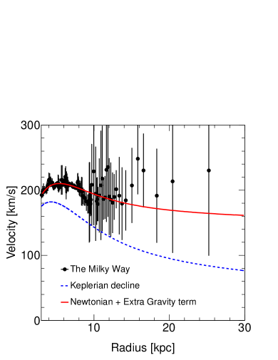
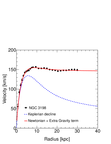
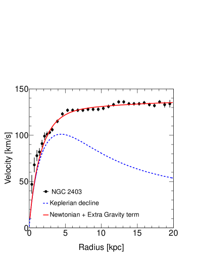
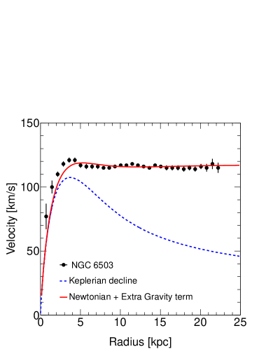
Figure 1: The predicted relationship between the galactic rotation speed $v$ and the distance $r$ from a combined influence of the Newtonian force and the new gravitational force: 1The Milky Way, 1NGC 3198, 1NGC 2403 and 1NGC 6503.

	The Milky Way	NGC 3198	NGC 2403	NGC 6503
$G\Sigma_{0}$ [$km^{2}s^{-2}kpc^{-1}$]	$6.8\times 10^{3}$	$2.8\times 10^{3}$	$2.1\times 10^{3}$	$2.8\times 10^{3}$
h [kpc]	2.0	2.63	2.05	1.72
$G^{\star}$ [kpc-2]	$5.0\times 10^{-2}$	$9.2\times 10^{-3}$	$1.4\times 10^{-2}$	$1.3\times 10^{-2}$
$\frac{m^{\prime}}{m}$	$2.3\times 10^{-9}$	$2.2\times 10^{-9}$	$2.0\times 10^{-9}$	$1.4\times 10^{-9}$

Table 1: The fitting parameters for some galaxies.

We also have to check for the influence of this diffuse halo medium on the motion of the planets in our solar system. With the values of the $G^{\star}$ and $m^{\prime}/m$ given in the above, the observed rotation speeds of the planets fit well with the predictions of Eq. 21. Figure 2 gives the planetary motions for various values of $G^{\star}$ and $m^{\prime}/m$.

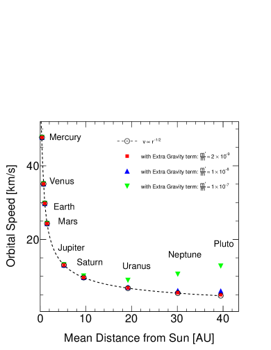
Figure 2: The orbital speeds of the planets in the solar system predicted by Eq. 21 with different $m^{\prime}/m$ values. $2\times 10^{-9}$, $1\times 10^{-8}$ and $1\times 10^{-7}$ are for red, blue and green points respectively.

The alert reader may find that, in the above discussions, we have already made the assumption that the stellar objects in the galaxies are composed solely of regular matter. This assumption can be understood in the following way. The primed matter always respond to the primed gravitational pull with a high rotation speed even when they are bound with some regular matter and hence are far harder for them to condense gravitationally into a star.

Though the stars contain no primed matter, the stars that are rotating at the outskirt of a spiral galaxy are, in fact, embedded in pockets of halo media and are rotating around the galaxy all together.

The amount of regular matter in the halo is small when compared with that in the galactic bulge and spiral arms, and is thus neglected in the above discussions.

6 Right amounts of intergalactic gravitational lensing

Next, let us turn to see what the primed matter does in explaining the large light deflections that are observed in intergalactic gravitational lensing. We shall take the galaxy cluster Abell 1689 as our illustration. We shall regard Abell 1689 as a cluster consisting of galaxies which are carrying their own individual halos with them. And this collection of galactic halos forms the halo of the cluster. Since the galactic halos are always regarded as having a size of the order of 30 kpc, the size of the cluster will be very close to its halo size which is taken to be 300 kpc.

The azimuthal angle swept by the light, when it travels from point $R$ to the point of closest approach $r_{0}$, under the influence of gravity described by the metric

$$ds^{2}=B(r)dt^{2}-A(r)dr^{2}-r^{2}d\Omega^{2},$$ (22)

is given by ref:19

$$\Delta\varphi\equiv\varphi(r_{0})-\varphi(R)=\int^{R}_{r_{0}}A^{\frac{1}{2}}(r)[(\frac{r}{r_{0}})^{2}\frac{B(r_{0})}{B(r)}-1]^{-\frac{1}{2}}\frac{dr}{r}.$$ (23)

In the case of the TPPN metric for a point source of primed mass $M^{\prime}$, the angle swept is

$$\Delta\varphi=\int^{R}_{r_{0}}\frac{(r_{0}+G^{\prime}M^{\prime})dr}{(r+G^{\prime}M^{\prime})[(r+G^{\prime}M^{\prime})^{2}-(r_{0}+G^{\prime}M^{\prime})^{2}]^{\frac{1}{2}}},$$ (24)

which can be readily integrated to give

$$\Delta\varphi=\sec^{-1}\frac{1+\beta R}{1+\beta r_{0}},$$ (25)

with $\beta$ = $\frac{1}{G^{\prime}M^{\prime}}$.

We will immediately notice that the angle change will be $\frac{\pi}{2}$ when $R$ goes to infinity. That means no deflection for the light by a point source of the primed matter when it comes from infinity and then goes back to infinity. Things will be different when we deal with a distributed source of the primed matter as we are going to show in the following.

Let $R$ be the radius of the halo of Abell 1689 and $r_{0}$ be the closest approach from the cluster center. The light will see a point source of the primed matter of constant mass $M^{\prime}$ when it is moving beyond the halo. And it will see a point source of diminishing mass (i.e. increasing $\beta$) when it enters the halo because it sees only the mass that lies inside $r$.

We claim that the deflection by a point source of mass $M^{\prime}$ is smaller than that by a uniformly distributed halo which has a total mass of $M^{\prime}$, if the light penetrates into the halo during some time in its journey. The above claim is obvious by noting that

$$\frac{d(\Delta\varphi)}{d\beta}>0.$$ (26)

So if the light penetrates into the cluster halo, the total azimuthal angle change will be greater than $\frac{\pi}{2}$, and we will see light deflectng towards the center of the cluster.

The actual angle swept, when light comes from the infinity, enters the halo at $R$ and reaches the point of closest approach at $r_{0}$ is given by

$$\frac{\pi}{2}+(\Delta\varphi|_{\rm{halo}}-\Delta\varphi|_{\rm{point\ source}}).$$ (27)

The second term in the bracket in Eq. 27 comes from the fact that we have to take out a $\frac{\pi}{2}$ in calculating the angle of deflection. The quantity inside the bracket of Eq. 27 can be regarded as a change $\delta(\Delta\varphi)$ in $\Delta\varphi$ due to a change $\delta M^{\prime}$ in $M^{\prime}$, and we get

$$\Delta\varphi|_{\rm{halo}}-\Delta\varphi|_{\rm{point\ source}}$$

$$=\delta(\Delta\varphi)$$

$$=\frac{\partial(\Delta\varphi)}{\partial M^{\prime}}\delta M^{\prime}$$ (28)

$$=\frac{\partial}{\partial M^{\prime}}[\sec^{-1}\frac{1+\beta R}{1+\beta r_{0}}]\delta M^{\prime}$$

$$=\frac{3}{\sqrt{2}}(R-r_{0})^{\frac{3}{2}}G^{\star-\frac{1}{2}}R^{-\frac{5}{2}}.$$

A plug in the data of $R$ = 300 kpc, $(R-r_{0})$ = 30 kpc and $G^{\star}$ = $10^{-2}$ $\mathrm{kpc^{-2}}$, will give us an angle of deflection, which is 2$\delta(\Delta\varphi)$, a value of $4\times 10^{-3}$, which is many times of that expected from General Relativity.

Note that the value of $G^{\star}$ that we used in calculating the Abell 1689 light deflection comes from the curve fittings of galactic rotations. Again there seems to be a universal value for $G^{\star}$, as it should be.

We should also note that the sun and the planets in the solar system aren’t contaminated with the primed matter as we have explained in the above. The fundamental tests on General Relativity will hence remain intact.

7 Primordial torsion and the accelerating expansion of the Universe

There is another nice feature of the Yang-Mills type gauge theory of gravity, when we use it to study the Universe as a whole. This theory was shown to admit a cosmological solution of the form ref:20 ; ref:21

$$ds^{2}=-dt^{2}+r_{0}^{2}e^{2\xi t}(dr^{2}+r^{2}d\theta^{2}+r^{2}\sin^{2}\theta d\phi^{2}),$$ (29)

with primordial local torsion compoments,

$$\tau_{\hat{0}\hat{1}\hat{1}}=\tau_{\hat{0}\hat{2}\hat{2}}=\tau_{\hat{0}\hat{3}\hat{3}}=\frac{\xi}{2}.$$ (30)

The $r_{0}$ and $\xi$, with $\xi>0$ are integration constants arising from the integration of the equation of motion. We can interpret this solution as representing an expanding and accelerating Universe when the influence of gravity dominates over the influence of matter and radiation. The role played by the primordial torsion is crucial here: the stretching on the Universe by the metric is compensated by the twisting by the torsion. And from the metrical point of view, we look like living in a Universe with a cosmological constant $\xi$. And interesting enough, our torsion selects the spatially flat metric ($\kappa$ = 0) as the only accompanying metric ref:20 ; ref:21 . The spatially flat geometry of the Universe is confirmed by WMAP. For more information on the predictions of the Yang-Mills type gauge theory of gravity on the evolution of the primordial Universe, the reader is referred to Ref. ref:22 .

8 Conclusion

The Yang-Mills type gauge theory of gravity has a richer structure than that of Einstein’s General Theory of Relativity. Its richer number of solutions, both in the absence and in the presence of torsion allow us to describe more physical phenomena with it. The recently observed astronomical Dark Matter and Dark Energy phenomena seems to show that Nature is enjoying the full use of the Yang-Mills type gauge theory of gravity.

Appendix A Superposition of two metrics

In this appendix we will cast the Stephenson Equation and the Stephenson-Kilmister-Yang Equation in static spherical symmetric forms. The metric is taken to be the form of Eq. 22, namely

$$ds^{2}=B(r)dt^{2}-A(r)dr^{2}-r^{2}d\Omega^{2}.$$ (1)

There are three independent, non-vanishing components for the left-hand-side of Eq. 9. They are, the $tt$ component,

$$8r^{2}A^{2}B^{2}B^{\prime 2}+r^{4}(A^{\prime}B^{\prime}B-AB^{\prime 2}-2AB^{\prime\prime}+2AB^{\prime 2})^{2}$$

$$-16A^{2}B^{4}(A-1)^{2}-8r^{2}A^{\prime 2}B^{4}=0,$$ (2)

the $rr$ component:

$$8r^{2}A^{\prime 2}B^{4}+r^{4}(A^{\prime}B^{\prime}B-AB^{\prime 2}-2ABB^{\prime\prime}+2AB^{\prime 2})^{2}$$

$$-16A^{2}B^{4}(A-1)^{2}-8r^{2}A^{2}B^{2}B^{\prime 2}=0,$$ (3)

the $\theta\theta$ component (same as the $\phi\phi$ component),

$$r^{4}(A^{\prime}B^{\prime}B-AB^{\prime 2}-2ABB^{\prime\prime}+2AB^{\prime 2})^{2}$$

$$-16A^{2}B^{4}(A-1)^{2}=0.$$ (4)

There are two independent components for the left-hand-side of Eq. 10. They are ref:7

$$r^{2}(2A^{2}B^{2}B^{\prime\prime\prime}-4A^{2}B^{\prime\prime}B^{\prime}B-3AA^{\prime}B^{2}B^{\prime\prime}+2A^{2}B^{\prime 3}$$

$$+2AA^{\prime}BB^{\prime 2}-AA^{\prime\prime}B^{2}B^{\prime}+2A^{\prime 2}B^{2}B^{\prime})$$

$$+2rAB(2ABB^{\prime\prime}-AB^{\prime 2}-A^{\prime}BB^{\prime})-4A^{2}B^{2}B^{\prime}$$

$$=0,$$ (5)

$$r^{2}(2AA^{\prime\prime}B^{2}+AA^{\prime}BB^{\prime}-4A^{\prime 2}B^{2})-4A^{2}B^{2}(A-1)=0.$$ (6)

Note that all these equations contain terms that are polynomials in $A$ and $B$.

Subtracting Eq. A from Eq. A will give

$$8r^{2}A^{2}B^{2}B^{\prime 2}-8r^{2}A^{\prime 2}B^{4}=8r^{2}A^{\prime 2}B^{4}-8r^{2}A^{2}B^{2}B^{\prime 2}$$ (7)

and will lead to

$$\frac{B^{\prime}}{B}=\pm\frac{A^{\prime}}{A}.$$ (8)

The primes appearing as suffices in Eq. 1 to Eq. 8 signify differentiations with respect to $r$.

Eq. 8 are the two solutions for the Schwarzchild metric and the TPPN metric, respectively. When we form the superposition of

$$g=\frac{M}{M+M^{\prime}}\bar{g}+\frac{M^{\prime}}{M+M^{\prime}}g^{\prime},$$ (9)

and if we use $B(r)$ and $A(r)$ to denote their $tt$ and $rr$ components of their metric then

$$B(r)=\bar{B}+\frac{M^{\prime}}{M}B^{\prime}$$

$$A(r)=\bar{A}+\frac{M^{\prime}}{M}A^{\prime}$$ (10)

in the limit of $\frac{M^{\prime}}{M}\to 0$. The bars and primes here are used to label the regular matter and the primed matter as we have mentioned in the article. Note that the above equations of Eq. 1 to 6 do not have $M$ and $M^{\prime}$, which appear in Eq. 9, as their coefficients because $M$ and $M^{\prime}$ are integration constants of the solutions. Substituting Eq. A into Eq. A, A, A, A and 6, and if we remember that $\bar{B}$ and $\bar{A}$ satisfy the original equations, then the left-hand-side of Eq. A, A, A, A and 6 will contain only terms that are proportional to $\frac{M^{\prime}}{M}$ or it higher orders. What that means is that for some given $M$ and $M^{\prime}$, and some given $\bar{B}$ and $\bar{A}$ satisfying the original equations, $B(r)$ and $A(r)$ will satisfy the equations approximately as far as $\frac{M^{\prime}}{M}$ is very small. That means the superposition given in Eq. 9 is an approximate solution to the equations as far as $\frac{M^{\prime}}{M}$ is very small. Similar arguments apply to the case when $\frac{M}{M^{\prime}}$ is very small.

- (1) H. Weyl, Ann. Phys. (Leipzig) 59, 101 (1919).
- (2) C. N. Yang, Phys. Rev. Lett. 33, 445 (1974).
- (3) G. Stephenson, Nuovo Cimento IX, 263 (1958).
- (4) F. W. Hehl, Erice Lecture 1979, Plenum Press, New York (1979).
- (5) Y. Yang and W. B. Yeung, arXiv:1205.2690 (2012).
- (6) For an analysis on the occurrence of unphysical states in gravity theories with torsion, see H. J. Yo and J. M. Nester, Int. J. Mod. Phys, D 747 (2002), and references therein.
- (7) A. H. Thomspson, Phys. Rev. Lett. 34, 507 (1975); R. Pavelle , Phys. Rev. Lett. 34, 1114 (1975).
- (8) C. Lanczos, Rev. Mod. Phys.21, 497 (1949); C. W. Kilmister Les Theories Relativistes de la Gravitation (Paris) (1962).
- (9) P. Baekler, P. Yasskin, General Relativity and Gravitation, 16 1135 (1984); W-T Ni, Phys. Rev. Lett. 35 319 (1975); erratum 35 1748 (1975); E. E. Fairchild, Jr., Phys. Rev. D, 384 (1976).
- (10) R. R. Hsu and W. B. Yeung, Chinese J. Phys.(Taiwan), 25 463 (1987).
- (11) A. Einstein, L. Infeld and B. Hoffmann, Ann. Math. 41, 455 (1940).
- (12) A. Toomre, Astrophys. J 138, 385 (1963).
- (13) P. Salucci, A. Lapi, C. Tonini, G. Gentile, I. Yegorova and U. Klein, Mon. Not. R. Astron. Soc. 378, 41 (2007) and references therein.
- (14) Y. Sofue, http://www.ioa.s.u-tokyo.ac.jp/~sofue/htdocs/2012DarkHalo/Table_GrandRC.dat.
- (15) R. Bottena, J. Gerritsen, Mon. Not. R. Astron Soc. 000 1 (1997).
- (16) Y. M. Lee, M. S. Chun, The J. of the Korean Astron Soc. 22 31 (1989).
- (17) M. E. Bacon, A. Sharrar, Eur. J. Phys. 31 479 (2010).
- (18) S. McGaugh, The Astro. J. 683 137 (2008).
- (19) S. Weinberg, Gravitation and Cosmology, John Wiley & Sons. Inc (1972).
- (20) H. H. Chen, R. R. Hsu and W. B. Yeung, Class. Quantum Grav. 2, 927 (1985). Simple inspection on the equations list in this paper will reveal that a = , h = k = and f = g = 0 readily solves the equations.
- (21) M. Q. Chen, D. C. Chen, R. R. Hsu and W. B. Yeung, Proceedings of the Nat. Sc. Council (Taiwan) 9, 10 (1985).
- (22) Y. Yang and W. B. Yeung, arXiv:1303.3801 (2013).