Analytic Investigation of the Branch Cut of the Green Function in Schwarzschild Space-time

Abstract

The retarded Green function for linear field perturbations in Schwarzschild black hole space-time possesses a branch cut in the complex-frequency plane. This branch cut has remained largely unexplored: only asymptotic analyses either for small-frequency (yielding the known tail decay at late times of an initial perturbation of the black hole) or for large-frequency (quasinormal modes close to the branch cut in this regime have been linked to quantum properties of black holes) have been carried out in the literature. The regime along the cut inaccessible to these asymptotic analyses has so far remained essentially unreachable. We present a new method for the analytic calculation of the branch cut directly on the cut for general-spin fields in Schwarzschild space-time. This method is valid for any values of the frequency on the cut and so it provides analytic access to the whole branch cut for the first time. We calculate the modes along the cut and investigate their properties and connection with quasinormal modes. We also investigate the contribution from these branch cut modes to the self-force acting on a point particle on a Schwarzschild background space-time.

I Introduction

The study of spin-field perturbations of black holes is important for many reasons. Classically they are important, for example, for investigating the classical stability of black holes, for the detection of field waves emitted by black holes and for the calculation of the self-force on a point particle moving in a black hole background space-time (which serves to model a black hole inspiral in the extreme mass ratio). Black hole perturbations are also important for understanding the quantum properties of black holes.

A crucial object for the study of Schwarzschild black hole perturbations is the retarded Green function of the wave equations they obey. These equations may be separated by performing a Fourier transform in time and a multipole decomposition in the angular separation of the spacetime points. Thus, the calculation of black hole perturbations is reduced to that of the Fourier modes in the complex-frequency ($\omega$) plane followed by a sum/integral of the modes. Leaver Leaver (1986a, 1988) deformed the Fourier integral along the real-frequency axis into the complex-frequency plane, thus picking up the singularities of the Fourier modes of the Green function. These modes possess two types of singularities as functions of complex frequency: an infinite number of simple poles (the so-called quasinormal mode frequencies) and a branch cut (BC) which lies on the negative-imaginary axis (NIA). Leaver showed that the two main contributions to the Green function then come from a series of modes (quasinormal modes, QNMs) at the poles and an integral of modes around the branch cut, which we shall refer to as BC modes. While QNMs have been extensively studied (see, e.g., Berti et al. (2009) for a review), very little is so far known about the BC modes.

To date, only the leading asymptotic behaviour of the BC modes for small frequencies along the NIA has been studied at length in the literature. This small-frequency regime in the BC is known to yield a leading power-law tail decay at late times of an initial black hole perturbation (see, e.g., the pioneering work by Price Price (1972a, b), details of the tail at large radius in Leaver (1986a) and details at arbitrary radius as well as a higher-order logarithmic behaviour in Casals and Ottewill (2012a); Casals and Ottewill ). The BC modes for large frequencies along the cut have only been studied by Maassen van den Brink Maassen van den Brink (2004) and by the authors Casals and Ottewill (2012b). In Casals and Ottewill (2012b) it was shown that the BC modes at large frequencies lead to a divergence in the BC contribution to both the Green function at ‘very early’ times as well as to the black hole response to a noncompact Gaussian distribution as initial data (it is expected these divergences in the BC contributions are cancelled by similar divergences in the QNM contributions). The fact that highly-damped QNMs approach the BC enabled Casals and Ottewill (2012a); Casals and Ottewill ; Maassen van den Brink (2004) to apply the large-frequency asymptotic analyses of the BC to the calculation of highly-damped QNMs. These modes have been associated to quantum properties of black holes (e.g., see Maggiore (2008) in relation to black hole area quantization and Keshet and Neitzke (2008) in relation to Hawking radiation in the case of rotating black holes).

To the best of our knowledge, the only investigations of the BC modes for frequencies which are neither asymptotically large nor small (we will refer to this regime as the ‘mid’-frequency regime) are the following ones, which were carried out in the gravitational case only. The BC in the Green function modes is due to a corresponding BC of a particular solution, $g_{\ell}(r,\omega)$, of the radial equation, Eq.(4) below. In Leung et al. (2003a, b) the authors obtained the radial solution $g_{\ell}(r,\omega)$ for frequencies near, but off, the NIA via a numerical integration of the radial equation. They thus calculated the radial solution on both sides of – but away from – the NIA, evaluated the difference and then extrapolated it onto the NIA, thus obtaining the BC ‘strength’. This is a rather tricky numerical evaluation, since the difference in values of $g_{\ell}$ between the two sides of the NIA becomes exponentially-small as the frequency approaches the NIA. The only other investigation of BC modes in the ‘mid’-frequency regime on the NIA was carried out by Maassen van den Brink who, in a different and impressive work Maassen van den Brink (2000), performed an asymptotic analysis of the BC modes about the so-called algebraically-special frequency $\omega_{AS}$ Wald (1973); Chandrasekhar (1984); Maassen van den Brink (2000).

The algebraically special frequency lying within the ‘mid’-frequency regime on the NIA occurs only for the case of field perturbations of spin $s=2$ (axial gravitational) and correspondingly the rest of this paragraph applies to this case only. The BC modes have a distinct ‘dipole-like’ behaviour near $\omega_{AS}$, unlike at other frequencies Leung et al. (2003a, b). The algebraically special frequency, though not a QNM itself for axial gravitational perturbations (it is a QNM for polar gravitational perturbations) Maassen van den Brink (2000) is intimately linked to QNMs: the dipole-like behaviour of the BC modes may be explained in terms of poles in the ‘unphysical’ complex-frequency Riemann sheet Leung et al. (2003a, b). Furthermore, a QNM frequency very close to (or exactly equal to) $\omega_{AS}$ marks the start of the highly-damped region of QNMs (e.g., Berti et al. (2009)). As the rotation of the black hole is increased from zero (i.e., the Schwarzschild case studied in this paper), multiplets of QNMs emerge from – exactly at or very near to, depending on the azimuthal angular number – the algebraically special frequency $\omega_{AS}$ Leung et al. (2003a, b); Berti et al. (2003), at least in the case of the lowest multipole angular momentum number $\ell=s=2$.

No analytic method exists so far for calculating the BC of the Green function in the ‘mid’-frequency regime (except, as mentioned above, near $\omega_{AS}$ for $s=2$). However, the above works (see Ref.18 in Leung et al. (2003a) and Sec.VI Maassen van den Brink (2000)) suggest the tantalizing possibility of calculating the BC by expressing the BC ‘strength’ via a convergent series of irregular confluent hypergeometric functions evaluated directly on the NIA, so that no extrapolation onto the NIA would be required. In this paper we take up this suggestion. Thus, we provide a new method for calculating analytically the BC modes for general integral spin directly on the NIA for arbitrary values of the frequency. We prove that our new series for the BC modes is convergent for any values of the frequency along the NIA, thus providing analytic access for the first time to the whole ‘mid’-frequency regime. We note that our method is also valid in the small- and large- frequency regimes, but it is not useful there since convergence becomes slower as the frequency becomes small while, for large-frequencies, the BC modes grow and oscillate for fixed radii. Asymptotic analyses are therefore necessary in practise in these regimes.

We calculate the BC modes using our new method and we investigate their properties and connection with QNMs. We also re-analyze the so-called Jaffé series (which is a series representation of the radial solution which is purely ingoing into the event horizon and possesses no BC) and, in particular, the behaviour of the Jaffé coefficients. Finally, we apply our calculation of the BC modes to investigate their contribution to the self-force (see, e.g., Poisson et al. (2011)) acting on a point particle moving on a Schwarzschild background space-time. In Casals and Ottewill (2012a) we ‘sketched out’ the main idea for our new method for the calculation of the BC modes for arbitrary frequency, in this paper we ‘flesh out’ the details. We note that the method we present here provided the results for the plots of quantities in the ‘mid’-frequency regime in Casals and Ottewill (2012b), where it was shown that these ‘mid’-frequency results overlap with the large-frequency asymptotics presented there. In Casals and Ottewill we will present a thorough small-frequency analysis of the BC modes and we will show that these ‘mid’-frequency results also overlap with that analysis in the small-frequency regime.

In Sec.II we introduce the main perturbation equations and expressions for the Green function modes. In Sec.III we present the various series representations which we use for the calculation of the BC modes; in particular, Eq.(17) is the new series that we derive and use for the calculation of the pivotal quantity, the BC ‘strength’. In Sec.IV we analyse the so-called Jaffé coefficients $a_{n}$ (in particular, we correct the large-$n$ asymptotics of these coefficients given in the literature), which are fundamental in the calculation of all the series representations we use. In Secs.V–VIII we calculate the various quantities required for the BC modes and these modes themselves. In Sec.IX we investigate the contribution of the BC modes to the self-force. Finally, in Appendix A we give some properties of the irregular confluent hypergeometric function, which we require for the calculation of the BC modes in the main body of the paper.

In this paper we take units $c=G=1$. We will frequently use a bar over a quantity to indicate that it has been made dimensionless via the introduction of an appropriate factor of the radius of the event horizon, $r_{h}=2M$, where $M$ is the mass of the black hole.

II Branch Cut

After a Fourier-mode decomposition in time $t$ and a multipole-$\ell$ decomposition in the angular distance $\gamma$, the retarded Green funcction for linear field perturbations in Schwarzschild space-time is expressed as

$$G_{ret}(x,x^{\prime})=\frac{1}{r\cdot r^{\prime}}\sum_{\ell=0}^{\infty}(2\ell+1)P_{\ell}(\cos\gamma)G^{ret}_{\ell}(r,r^{\prime};t),\quad G^{ret}_{\ell}(r,r^{\prime};t)\equiv\frac{1}{2\pi}\int_{-\infty+ic}^{\infty+ic}d\omega\ G_{\ell}(r,r^{\prime};\omega)e^{-i\omega t},$$ (1)

where $c>0$ and the Fourier modes of the Green function are given by

$$G_{\ell}(r,r^{\prime};\omega)=\frac{f_{\ell}(r_{<},\omega)g_{\ell}(r_{>},\omega)}{W\left(\omega\right)},$$ (2)

where $r_{>}\equiv\max(r,r^{\prime}),\ r_{<}\equiv\min(r,r^{\prime})$ and $r$ is the Schwarzschild radial coordinate. The function

$$W\left(\omega\right)\equiv W\left[g_{\ell}(r,\omega),f_{\ell}(r,\omega)\right]=g_{\ell}f_{\ell}^{\prime}-f_{\ell}g_{\ell}^{\prime},$$ (3)

where a prime indicates a derivative with respect to $r_{*}$, is the Wronskian of two solutions $f_{\ell}(r,\omega)$ and $g_{\ell}(r,\omega)$ of the following second order radial ODE:

$$\left[\frac{d^{2}}{dr_{*}^{2}}+\omega^{2}-V(r)\right]u_{\ell}(r,\omega)=0$$ (4)

$$V(r)\equiv\left(1-\frac{r_{h}}{r}\right)\left[\frac{\ell(\ell+1)}{r^{2}}+\frac{r_{h}(1-s^{2})}{r^{3}}\right]$$

where $r_{*}\equiv r+r_{h}\ln\left(\frac{r}{r_{h}}-1\right)$ is the radial ‘tortoise coordinate’, $r_{h}\equiv 2M$ is the radius of the event horizon and $M$ is the mass of the Schwarzschild black hole. For $\omega\in\mathbb{R}$, the solutions $f_{\ell}$ and $g_{\ell}$ obey the ‘physical’ boundary conditions of, respectively, purely-ingoing waves into the black hole

$$f_{\ell}(r,\omega)\sim e^{-i\omega r_{*}}, \bar{r}_{*}\to-\infty,$$ (5)

$$f_{\ell}(r,\omega)\sim A^{out}_{\ell,\omega}e^{+i\omega r_{*}}+A^{in}_{\ell,\omega}e^{-i\omega r_{*}}, \bar{r}_{*}\to+\infty$$ (6)

and purely-outgoing waves out to radial infinity,

$$g_{\ell}(r,\omega)\sim e^{+i\omega r_{*}},\quad\ \bar{r}_{*}\to\infty$$ (7)

The complex-valued coefficients $A^{in}_{\ell,\omega}$ and $A^{out}_{\ell,\omega}$ are, respectively, incidence and reflection coefficients and it is straight forward to check that $W=-2i\omega A^{in}_{\ell,\omega}$. The boundary conditions (5) and (7) also define, respectively, the radial solutions $f_{\ell}$ and $g_{\ell}$ unambiguously for $\text{Im}(\omega)\geq 0$ when $r_{*}\in\mathbb{R}$. In $\text{Im}(\omega)<0$, with $r_{*}\in\mathbb{R}$ , the solution $g_{\ell}$ must be defined by analytic continuation.

The parameter $s=0,1,2$ in the potential in Eq.(4) is the helicity of the field perturbation, to which, with an abuse of language, we will refer to as ‘spin’: $s=2$ corresponds to axial – also called ‘odd’ – gravitational perturbations (in which case Eq.(4) becomes the Regge-Wheeler equation Regge and Wheeler (1957)), $s=1$ to electromagnetic perturbations Wheeler (1955) and $s=0$ to scalar perturbations Price (1972a, b). Polar – or ‘even’ – gravitational perturbations obey the Zerilli equation Zerilli (1970a, b) and solutions to this equation can be obtained from the solutions, and their radial derivatives, to the Regge-Wheeler equation Chandrasekhar (1983). At the algebraically special frequency $\omega_{AS}$ Wald (1973); Chandrasekhar (1984); Maassen van den Brink (2000), however, this relationship between solutions to the Zerilli equation and solutions to the Regge-Wheeler equation becomes singular. In Fig.1 we plot the potential $V(r)$ for some token values of spin $s$ and multipole number $\ell$.

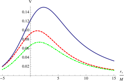
Figure 1: Radial potential Eq.(4) as a function of $r_{*}/M$. Continuous blue curve: $s=2$, $\ell=2$; dot-dashed green curve: $s=1$, $\ell=1$; dashed red curve: $s=0$, $\ell=1$.

It can be shown Leaver (1986b) that the radial solution $f_{\ell}$ has no branch cut in the complex-frequency plane whereas $g_{\ell}$ has a branch cut down the negative imaginary axis NIA (see, e.g., Eq.(13) below). This BC in $g_{\ell}$ can be explained Ching et al. (1995a, b) in terms of the radial potential (minus the centrifugal barrier) falling off slower than exponentially at radial infinity. On the other hand, the exponential decay with $r_{*}$ of the potential near the horizon leads to a series of poles in $f_{\ell}$ down in the NIA (see Sec.V below). We note that the Wronskian $W$ ‘inherits’ the BC from $g_{\ell}$ and the poles in the NIA from $f_{\ell}$. We define $\Delta A(\nu)\equiv A_{+}(-i\nu)-A_{-}(-i\nu)$ for any function $A=A(\omega)$ possessing a BC along the NIA, where $A_{\pm}(-i\nu)\equiv\lim_{\epsilon\to 0^{+}}A(\pm\epsilon-i\nu)$, with $\nu>0$. We will equally refer to both quantities $\omega$ and $\nu\equiv i\omega$ as ‘frequencies’; we note that $\nu>0$ along the NIA.

We note the symmetries

$$g_{\ell}(r,\omega)=g_{\ell}^{*}(r,-\omega^{*}),\quad f_{\ell}(r,\omega)=f_{\ell}^{*}(r,-\omega^{*}),\quad W(\omega)=W^{*}(-\omega^{*})\quad\text{if}\quad r_{*}\in\mathbb{R}$$ (8)

which follow from the radial ODE (4) and the boundary conditions (5) and (7). These symmetries lead to $g_{\ell-}=g_{\ell+}^{*}$ and $W_{+}=W_{-}^{*}$ if $r_{*}\in\mathbb{R}$, so that the branch cuts of $g_{\ell}(r,\omega)$ and $W$ along the NIA are only in their imaginary parts, their real parts having no branch cut. In particular, then, the absolute value of the Wronskian, $|W|$, has no BC.

The Fourier integral along the real frequency line in Eq.(1) can be deformed into the complex-frequency plane Leaver (1986a, 1988). The two main contributions to $G^{ret}_{\ell}$ are, then, a series over the residues at the poles of the Fourier modes $G_{\ell}(r,r^{\prime};\omega)$ (the QNM frequencies, which are located at the zeros of the Wronskian $W$) and an integral around the BC. The branch cut contribution $G^{BC}$ to the retarded Green function is given by

$$G^{BC}(r,r^{\prime};\gamma;t)=\frac{1}{r\cdot r^{\prime}}\sum_{\ell=0}^{\infty}(2\ell+1)P_{\ell}(\cos\gamma)G^{BC}_{\ell}(r,r^{\prime};t),\quad G_{\ell}^{BC}(r,r^{\prime};t)\equiv-\frac{i}{2\pi}\int_{0}^{-\infty}d\nu\ \Delta G_{\ell}(r,r^{\prime};\nu)e^{-\nu t},$$ (9)

where the BC modes $\Delta G_{\ell}$ can be expressed as Casals and Ottewill (2012b); Leung et al. (2003a)

$$\Delta G_{\ell}(r,r^{\prime};\nu)=-2i\nu f_{\ell}(r,-i\nu)f_{\ell}(r^{\prime},-i\nu)\frac{q(\nu)}{|W|^{2}},\quad r_{*}\in\mathbb{R}$$ (10)

We denote the function $q(\nu)$ as the branch cut ‘strength’ as it is defined via the equation

$$\Delta\tilde{g}_{\ell}(r,\nu)=iq(\nu)g_{\ell}(r,+i\nu).$$ (11)

where, here, $\Delta\tilde{g}_{\ell}(r,\nu)\equiv g_{\ell+}(r,-i\nu)-g_{\ell-}(r,-i\nu)$ (the extra tilde in the notation is justified in the next section). From the symmetries (8) and the fact that $g_{\ell}(r,+i\nu)$ (that is, $g_{\ell}$ evaluated on the positive-imaginary axis) is real-valued it follows that $q(\nu)$ is also a real-valued quantity. We note that ‘$-iq$’ here corresponds to the quantity ‘$K$’ in Eq.31 Leaver (1986a).

As mentioned in the Introduction, we will use a bar over a quantity to indicate that it has been made dimensionless via the introduction of an appropriate factor $r_{h}$, e.g., $\bar{r}\equiv r/r_{h}$, $\bar{\omega}\equiv\omega r_{h}$, $\bar{\nu}\equiv\nu r_{h}$, etc.

III Series representations for the radial solutions

If one tried to find the radial solution $f_{\ell}$ or $g_{\ell}$ in the region $\text{Im}(\omega)<0$ by naïvely solving numerically the radial Eq.(4) and imposing the ‘boundary conditions’ (5) and (7), respectively, one would run into computational problems. The reason is that these ‘boundary conditions’ are exponentially dominant over the other, linearly independent solution at the radial endpoint where the condition is imposed (that is, at $\bar{r}_{*}\to-\infty$ for $f_{\ell}$ and at $\bar{r}_{*}\to+\infty$ for $g_{\ell}$). Therefore, if one tried to numerically integrate the radial ODE starting with the ‘boundary condition’ at one endpoint towards the other endpoint, any accidental inclusion – no matter how small – of the other, wrong solution would grow exponentially and so would the numerical error. There are various methods around this problem. For example, one could solve the radial equation in the region $\text{Im}(\omega)\geq 0$, where the boundary conditions are well-posed, and then analytically continue onto the region $\text{Im}(\omega)<0$. Also, Leaver’s Eqs.32–36 Leaver (1986a) provides a framework for calculating the BC contribution to the retarded Green function. However, this method is rather difficult to implement (except in the asymptotic small-$\bar{\nu}$ regime) due to the presence of Leaver’s ‘phase parameter’, which is required because of the use of a particular series representation for $g_{\ell}$ in terms of Coulomb wave functions. In this paper we choose to use certain series representations for $f_{\ell}$ and $g_{\ell}$ which do not involve Leaver’s ‘phase parameter’ and which we show are convergent in the desired region on the frequency plane.

Leaver Leaver (1986b) provides various series representations for the radial solutions $f_{\ell}$ and $g_{\ell}$. All calculations of the BC modes in this paper are carried using a specific choice of series representation for each one of the two solutions, which we give in Secs.III.1 and III.2. However, while the new series representation for $\Delta\tilde{g}_{\ell}$ (and therefore for the BC ‘strength’ $q(\nu)$) which we present in Sec.III.3 is fundamentally based on our choice of series representation for $g_{\ell}$, our calculation of the BC modes does not depend in an important way on the specific choice of series for calculating $f_{\ell}$: one could just as well use any different method valid in the ‘mid’-frequency regime for calculating $f_{\ell}$. We present the various series that we use in the following subsections and we investigate their convergence properties in the following sections.

III.1 Series for $f_{\ell}$

In order to calculate the radial function $f_{\ell}$, we will use the well-known Jaffé series Leaver (1986b)

$$f_{\ell}(r,\omega)=\left(\bar{r}-1\right)^{-i\bar{\omega}}\bar{r}^{2i\bar{\omega}}e^{i\omega r}J_{\ell}(r,\omega),$$ (12)

$$J_{\ell}(r,\omega)\equiv\sum_{n=0}^{\infty}J_{n,\ell}(\omega),\quad J_{n,\ell}\equiv a_{n}(\omega)\left(1-\frac{1}{\bar{r}}\right)^{n}$$

We will refer to the complex-valued coefficients $a_{n}(\omega)$ as the Jaffé series coefficients, even though they also appear as coefficients in the series representation that we will use for $g_{\ell}$, Eq.(13) below. The Jaffé series coefficients are functions of the series index $n$, the frequency $\omega$ and, although not indicated explicitly, the multipole number $\ell$ and the spin value $s$. The Jaffé series coefficients satisfy a 3-term recurrence relation which we give and analyze in the following section. The initial value $a_{0}$ remains undetermined by the recurrence relation; the specific value $a_{0}=e^{-2i\bar{\omega}}$ yields the desired normalization (5) for $f_{\ell}$ and, therefore, this will always be our choice of value for $a_{0}$ when using the Jaffé series for $f_{\ell}$.

III.2 Series for $g_{\ell}$

Our choice of series representation for $g_{\ell}$ is also given in Leaver (1986b):

$$g_{\ell}(r,\omega)=\bar{r}^{1+s}\left(\bar{r}-1\right)^{-i\bar{\omega}}e^{i\omega r}h_{\ell}(r,\omega),\quad h_{\ell}(r,\omega)\equiv\sum_{n=0}^{\infty}h_{n,\ell}(\omega),\qquad h_{n,\ell}\equiv\tilde{a}_{n}(\omega)T_{n}^{(-)}$$ (13)

$$T_{n}^{(-)}\equiv(-2i\bar{\omega}+1)_{n}\ U(s+1-2i\bar{\omega}+n,2s+1,-2i\omega r),$$

where $\tilde{a}_{n}(\omega)$ satisfy the same recurrence relations as the Jaffé series coefficients $a_{n}$ in Eq.(12) but it is $\tilde{a}_{0}\neq a_{0}$ – that is, $\tilde{a}_{n}$ and $a_{n}$ only differ by an overall normalization factor which we give below. The series (13) has been broadly ignored in the literature, possibly due to the fact that the irregular confluent hypergeometric $U$-functions are rather hard to manage. We will refer to Eq.(13) as the ‘Leaver-$U$ series’.

It is clear from the Leaver-$U$ series Eq.(13) and the properties of the irregular confluent hypergeometric function bk: that the radial solution $g_{\ell}(r,\omega)$ has a branch cut running along the line $\omega r:0\to-\infty\cdot i$. If $r>0$, then $g_{\ell}(r,\omega)$ has a branch cut along the NIA, $\omega:0\to-\infty\cdot i$.

The principal branch of $U(a,b,z)$ is given by $\arg(z)\in(-\pi,+\pi]$. Therefore, we can evaluate directly on the NIA the confluent hypergeometric $U$-function appearing in Eq.(13) and calculate the corresponding $T_{n}^{(-)}$ via Eq.(13). That is, $T_{n}^{(-)}$ may be evaluated on the NIA and its value will correspond to the principal branch value, i.e., to the limiting value as the frequency $\omega$ approaches the NIA from the third quadrant in the complex-frequency plane. The corresponding value of $g_{\ell}$ will then give $g_{\ell+}$ provided that the series Eq.(13) converges. It will be understood, when we do not say it explicitly, that any quantities possessing a BC along the NIA which are evaluated on the NIA via the use of Eq.(13) will correspond to their limiting value approaching the NIA from the third quadrant.

In order to check what boundary condition the Leaver-$U$ series (13) satisfies for $r\to\infty$, we use Eq.13.5.2 Abramowitz and Stegun (1972) and we obtain

$$g_{\ell}(r,\omega)\sim\bar{r}^{1+s}\left(\bar{r}-1\right)^{-i\bar{\omega}}(-2i\omega r)^{-s-1+2i\bar{\omega}}\tilde{a}_{0}e^{+i\omega r}\quad\text{for}\ |\omega r|\to\infty\ \text{and}\ |\pi/2-\arg(\omega)-\arg(r)|<3\pi/2$$ (14)

Therefore, when $r>0$, the Leaver-$U$ series yields the asymptotics

$$g_{\ell}(r,\omega)\sim(-2i\bar{\omega})^{-s-1+2i\bar{\omega}}\tilde{a}_{0}e^{+i\omega r_{*}}\quad\text{for}\ r\to\infty\ \text{and}\ |\pi/2-\arg(\omega)|<3\pi/2,\quad r>0$$ (15)

We note that Eq.(15) does not agree with Eq.75 Leaver (1986b); we believe that Eq.75 Leaver (1986b) is missing the first factor on the right hand side of Eq.(15).

With the specific normalization choice of $\tilde{a}_{0}=(-2i\bar{\omega})^{+s+1-2i\bar{\omega}}$ the function $g_{\ell}$ calculated using the Leaver-$U$ series satisfies the desired normalization Eq.(7); therefore, this will always be our choice (different from the choice $a_{0}=e^{-2i\bar{\omega}}$ above for the Jaffé series for $f_{\ell}$) when using the Leaver-$U$ series for $g_{\ell}$. We note that $\tilde{a}_{n}$ themselves have a branch cut along the NIA (this was already noted in Ref.18 of Leung et al. (2003a)), as we have

$$\Delta\tilde{a}_{n}=\left[e^{-4\pi\bar{\omega}}-1\right]\tilde{a}_{n-}=\left[e^{4\pi\bar{\omega}}+1\right]\tilde{a}_{n+}$$ (16)

where $\tilde{a}_{n\pm}\equiv\lim_{\epsilon\to 0^{+}}\tilde{a}_{n}(\omega=\pm\epsilon-i\nu)$ and where we have assumed $s\in\mathbb{Z}$.

III.3 Series for $\Delta\tilde{g}_{\ell}$

From Eqs.(13) and (39) it follows that

$$\Delta\tilde{g}_{\ell}(r,\nu)\equiv g_{\ell+}(r,-i\nu)-g_{\ell-}(r,-i\nu)=\bar{r}^{1+s}\left(\bar{r}-1\right)^{-\bar{\nu}}e^{\nu r}\Delta\tilde{h}_{\ell}(r,\nu),\quad\Delta\tilde{h}_{\ell}(r,\nu)=\sum_{n=0}^{\infty}\Delta\tilde{h}_{n,\ell}$$ (17)

$$\Delta\tilde{h}_{n,\ell}\equiv\frac{2\pi ie^{-2\nu r}e^{\pi i(s+1-2\bar{\nu})}}{\Gamma(1-2\bar{\nu})}\tilde{a}_{n-}\cdot T_{n}^{(0)},\quad T_{n}^{(0)}\equiv\frac{(-1)^{n}\Gamma(1+n-2\bar{\nu})U(s-n+2\bar{\nu},2s+1,2\nu r)}{\Gamma(1+s+n-2\bar{\nu})\Gamma(1-s+n-2\bar{\nu})}$$

This is a series for calculating $\Delta\tilde{g}_{\ell}$ by evaluating quantities directly on the NIA. The principal branch is to be taken for the confluent hypergeometric $U$-function in Eq.(17).

III.4 Series for $\Delta g_{\ell}$

The series in this subsection, which we denote by $\Delta g_{\ell}$, would correspond to $\Delta\tilde{g}_{\ell}$ if the coefficients $\tilde{a}_{n}$ did not have a branch cut; specifically, we may view $\Delta g_{\ell}$ as the discontinuity of $g_{\ell}$ across the NIA if we replace $\tilde{a}_{n}$ by $a_{n}$ in Eq.(13). Since that is not actually the case, we will not be using the series for $\Delta g_{\ell}$ anywhere. However, we include it here for completeness, as the factors $T_{n}^{(+)}$ in the terms of this series satisfy the same recurrence relation (Eq.(26) below) as the factors $T_{n}^{(-)}$ and $T_{n}^{(0)}$ introduced above for $g_{\ell}$ and $\Delta\tilde{g}_{\ell}$ respectively. The solution $T_{n}^{(+)}$ to the recurrence relation Eq.(26) is linearly independent from the solutions $T_{n}^{(-)}$ and $T_{n}^{(0)}$. If we replace $\tilde{a}_{n}$ by $a_{n}$ in Eq.(13), we can calculate the discontinuity across the NIA of the resulting quantity as:

$$\Delta g_{\ell}(r,\nu)\equiv g_{\ell+}(r,-i\nu)\frac{a_{{n}+}}{\tilde{a}_{n+}}-g_{\ell-}(r,-i\nu)\frac{a_{{n}-}}{\tilde{a}_{n-}}=\bar{r}^{1+s}\left(\bar{r}-1\right)^{-\bar{\nu}}e^{+\nu r}\Delta h_{\ell}(r,\nu),\quad\Delta h_{\ell}(r,\nu)=\sum_{n=0}^{\infty}\Delta h_{n,\ell}$$ (18)

$$\Delta h_{n,\ell}\equiv\frac{(-1)^{2s}2\pi ia_{n}}{\Gamma(1+2s)\Gamma(1-2\bar{\nu})}T_{n}^{(+)},\quad T_{n}^{(+)}\equiv\frac{\Gamma(1-2\bar{\nu}+n)M(1-2\bar{\nu}+n+s,2s+1,-2\nu r)}{\Gamma(1-2\bar{\nu}+n-s)}$$

where we have used Eq.13.1.6 in Abramowitz and Stegun (1972). We note the appearance of the regular confluent hypergeometric (Kummer) function $M$ in (18) for $\Delta g_{\ell}$, as opposed to the irregular confluent hypergeometric function $U$ in Eq.(17) for $\Delta\tilde{g}_{\ell}$.

III.5 Series for the radial derivatives

An expression for calculating the $r_{*}$-derivative of the radial solution $f_{\ell}$ follows straightforwardly from Eq.(12):

$$\frac{df_{\ell}}{dr_{*}}=\left(\bar{r}-1\right)^{1-\bar{\nu}}\bar{r}^{2\bar{\nu}-1}e^{\nu r}\left[\frac{dJ_{\ell}}{dr}+\nu\frac{(\bar{r}^{2}-2)}{\bar{r}(\bar{r}-1)}J_{\ell}\right]$$ (19)

$$\frac{dJ_{\ell}}{dr}=\frac{1}{r_{h}\bar{r}^{2}}\sum_{n=0}^{\infty}(n+1)a_{n+1}\left(1-\frac{1}{\bar{r}}\right)^{n}$$

In order to obtain an expression for the $r_{*}$-derivative of $g_{\ell}$ we use Eqs.4.22–4.24 Liu (1997):

$$\frac{dg_{\ell}}{dr_{*}}=\left(1-\frac{1}{\bar{r}}\right)\left[\left(\frac{1+s}{r}-\frac{\bar{\nu}}{r-r_{h}}+\nu\right)g_{\ell}+\frac{g_{\ell}}{h_{\ell}}\frac{dh_{\ell}}{dr}\right]$$ (20)

$$\frac{dh_{\ell}}{dr}=\sum_{n=0}^{\infty}\tilde{a}_{n}\frac{dT_{n}^{(-)}}{dr},\quad\frac{dT_{n}^{(-)}}{dr}=\frac{s+1-2\bar{\nu}+n}{r}\left[\frac{-2\bar{\nu}+n+1-s}{-2\bar{\nu}+n+1}T_{n+1}^{(-)}-T_{n}^{(-)}\right]$$

IV Jaffé series coefficients

Both the series coefficients $a_{n}(\omega)$ appearing in the Jaffé series Eq.(12) for $f_{\ell}$ and the series coefficients $\tilde{a}_{n}(\omega)$ appearing in the Leaver-$U$ series Eq.(13) for $g_{\ell}$ satisfy the following 3-term recurrence relation,

$$\alpha_{n}a_{n+1}+\beta_{n}a_{n}+\gamma_{n}a_{n-1}=0,\quad n=1,2,\dots$$ (21)

with $a_{n}=0$ for $n<0$ and where

$$\alpha_{n} \equiv(n+1)(n-2\bar{\nu}+1)$$

$$\beta_{n} \equiv-[2n^{2}+(2-8\bar{\nu})n+8\bar{\nu}^{2}-4\bar{\nu}+\ell(\ell+1)+1-s^{2}]$$ (22)

$$\gamma_{n} \equiv n^{2}-4\bar{\nu}n+4\bar{\nu}^{2}-s^{2}$$

We note that although in this section we use the notation $a_{n}$ to indicate a solution of Eq.(21) the results in this section apply equally to the coefficients $\tilde{a}_{n}$ since these results are independent of the specific choice of the $n=0$ coefficient.

IV.1 Singularities of $a_{n}$

From Eq.(21) it follows that, in principle, the coefficients $a_{n}$ will have a simple pole where $\alpha_{n-1}=0$, i.e., at $n-2\bar{\nu}=0$. Therefore, if $\bar{\nu}=k/2$ for some $k\in\mathbb{N}$ then $a_{n}$ will have a simple pole $\forall n\geq k$ (see, e.g., App.B Leung et al. (2003a)). However, such a pole will not occur if at the same time it happens that $\beta_{k-1}a_{k-1}+\gamma_{k-1}a_{k-2}=0$. This occurs for $s=2$ at the algebraically-special frequency $\bar{\omega}_{AS}=-i\bar{\nu}_{AS}$, where $\bar{\nu}_{AS}\equiv(\ell-1)\ell(\ell+1)(\ell+2)/6$ Maassen van den Brink (2000). Therefore, the coefficients $a_{n}$ do not have a pole at $\bar{\nu}=\bar{\nu}_{AS}$ for $s=2$ while they do have a simple pole there for $s=0,1$.

Suppose that $\left\{b_{n}\right\}$ and $\left\{c_{n}\right\}$ are two sets of solutions to a recurrence relation, then, if $\lim_{n\to\infty}b_{n}/c_{n}=0$ it is said that $b_{n}$ are minimal and $c_{n}$ are dominant. If the solution one seeks is dominant, then one can find the desired solution by solving the recurrence relation using standard forward recursion. However, if one wants to obtain a minimal solution, using forward recursion would be unstable and one must resort to finding the desired solution using, e.g., Miller’s algorithm of backward recursion (see, e.g., Gautschi (1961)). In order to investigate whether the solutions to the recurrence relation Eq.(21) are minimal, dominant or neither, we require the large-$n$ behaviour of the coefficients $a_{n}$. We also require the large-$n$ behaviour of $a_{n}$ in order to study the convergence properties of any series involving these coefficients.

IV.2 Large-$n$ asymptotics

In order to obtain the large-$n$ asymptotics of the coefficients $a_{n}$ we follow App.B Wimp (1984). We thus express the asymptotic behaviour as the so-called Birkhoff series

$$a_{n}=e^{\mu_{0}n\ln n+\mu_{1}n}n^{\zeta_{0}}e^{\sum_{j=0}^{I}\zeta_{j+1}n^{\beta-j/\rho}+O\left(n^{\beta-(I+1)/\rho}\right)}$$ (23)

for a certain chosen value of $I\in\mathbb{N}$, where $\beta\in[0,1)$, $\zeta_{1}\neq 0$, $\rho\in\mathbb{Z}$, $\rho\geq 1$ and $\mu_{j},\zeta_{j}\in\mathbb{C}$ for all $j$. Substituting this expression into the recurrence relation (21) we obtain

$$a_{n}=n^{-\bar{\nu}-3/4}e^{\pm 2\sqrt{2\bar{\nu}n}i+\sum_{j=1}^{I}\zeta_{j+1}n^{1/2-j/2}+O\left(n^{1/2-(I+1)/2}\right)}$$ (24)

$$\zeta_{3}=\frac{i(-9-48\ell-48\ell^{2}-48\bar{\nu}+64\bar{\nu}^{2})}{48\sqrt{2}\sqrt{\bar{\nu}}}$$

$$\zeta_{4}=\frac{3+16\ell+16\ell^{2}-48\bar{\nu}+64s^{2}\bar{\nu}+128\bar{\nu}^{2}+128\bar{\nu}^{3}}{128\bar{\nu}}$$

$$\zeta_{5}=$$

$$\frac{i}{30720\sqrt{2}\bar{\nu}^{3/2}}\left[315-1280\ell^{4}-2560\ell^{3}+160\ell^{2}+1440\ell+\left(7680\ell^{2}+7680\ell+13728\right)\bar{\nu}+\right.$$

$$\left.\left(-30720\ell^{2}-30720\ell-3200\right)\bar{\nu}^{2}-10240\bar{\nu}^{3}\right]$$

$$\zeta_{6}=$$

$$\frac{1}{24576\bar{\nu}^{2}}\left[-81+768\ell^{4}+1536\ell^{3}+480\ell^{2}-288\ell+\left(-1536\ell^{2}-1536\ell-288\right)\bar{\nu}+\left(6144\ell^{2}+6144\ell+1152\right)\bar{\nu}^{2}+\right.$$

$$\left.\left(24576s^{2}-16384\right)\bar{\nu}^{3}+24576\bar{\nu}^{4}+16384\bar{\nu}^{5}\right]$$

The coefficients $\zeta_{j}$ are real for $j$ even and they are purely imaginary for $j$ odd . We note that the spin dependence does not appear until the term $\zeta_{6}$. The coefficient $\zeta_{2}$ corresponds to an undetermined overall normalization and the ‘$\pm$’ sign corresponds to the two linearly independent solutions of the recurrence relation. Since the recurrence relation (21) is unchanged under $n\to ne^{2\pi i}$, one solution can be obtained from the other under this change; this is essentially equivalent to changing the sign of $\zeta_{j+1}$ for $j$ even in (24). On the NIA, where $\bar{\nu}>0$, the two solutions behave similarly (that is, no solution is dominant over the other) and an appropriate linear combination of them should be taken. Off the NIA, if $\omega$ is not a QNM frequency then the $a_{n}$ are dominant Leaver (1986a) and they are generated by forward recursion; whereas if $\omega$ is a QNM frequency then the $a_{n}$ are minimal and they can be generated by Miller’s algorithm of backward recursion. Indeed, requiring for the solutions $a_{n}$ to be minimal has become a widely used, successful method for finding QNM frequencies of black holes Leaver (1985).

Finally, we note that the leading order of Eq.(24) differs from Eq.46 Leaver (1986b) in having a power of $n$ equal to ‘$-\bar{\nu}-3/4$’ instead of ‘$-2\bar{\nu}-3/4$’; we have checked numerically for specific values of the parameters (both for $\omega$ on and off the NIA) that Eq.(24) gives the correct asymptotic behaviour.

IV.3 Plots

In Fig.2 we show that the large-$n$ asymptotics given in Eq.(24) match the exact solution to the recurrence relation (21). We note the appearance of a ‘pulse’, after which the values of $a_{n}$ decay rapidly. Fig.3 is a 3D-plot of $a_{n}$ as a function of both $n$ and $M\nu$. We have only included plots for $s=2$ as representative of the behaviour of the coefficients $a_{n}$, as the behaviour is similar for other spins. The behaviour is also similar at the algebraically-special frequency $\omega_{AS}$. At the poles described in Sec.IV.1 the behaviour of ‘$\sin(2\pi\bar{\nu})a_{n}$’ is also similar, except that the first $n<2\bar{\nu}$ terms are exactly zero.

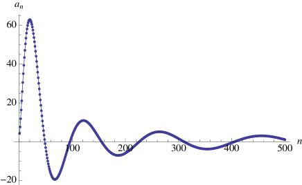
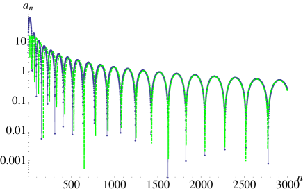
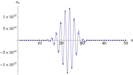
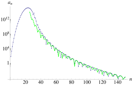
Figure 2: Jaffé coefficient $a_{n}$ as a function of $n$ for $s=2$, $\ell=2$. Figs.(a) and (b) are for $\bar{\nu}=0.2$ and figs.(c) and (d) for $\bar{\nu}=15.4$. Figs. (b) and (d) are log-plot versions of (a) and (c) respectively. Blue dots: exact solution $a_{n}$ to the recurrence relation (21) with $a_{0}=1$; the continuous blue curve is an interpolation of the blue dots. Dashed green curve: large-$n$ asymptotics Eq.(24) where we have taken a linear combination of the two linearly independent asymptotic solutions such that the linear combination matches the exact value of $a_{n}$ at both $n=1000$ and $n=2000$ for $\bar{\nu}=0.2$, and at $n=145$ and $n=150$ for $\bar{\nu}=15.4$. We note the ‘pulse’ centered around $n=25$ in the case $\bar{\nu}=15.4$ (the equivalent ‘pulse’ in the case $\bar{\nu}=0.2$ is centered around its first peak at $n\approx 20$); the coefficient $a_{n}$ reaches its maximum magnitude at the ‘pulse’ and then the magnitude decays rapidly with $n$.

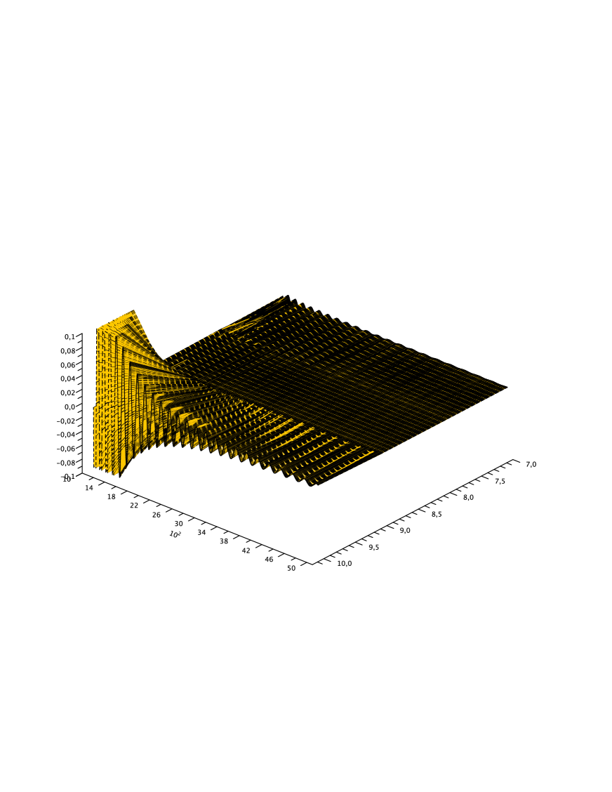
Figure 3: Exact solution $a_{n}$ to the recurrence relations with $s=0$, $\ell=2$ as a function of both $M\nu:7.1001\to 10.1001$ and $n=1000\to 5000$.

V Calculation of $f_{\ell}(r,\omega)$

We calculate the radial solution $f_{\ell}$ using the Jaffé series Eq.(12). As shown by Leaver in Sec.IV.A Leaver (1986b), the Jaffé series is absolutely convergent $\forall\omega\in\mathbb{C}$ and for any $r\in[r_{h},\infty)$, since then: $\lim_{n\to\infty}\left|a_{n+1}(1-1/\bar{r})^{n+1}/(a_{n}(1-1/\bar{r})^{n})\right|=|1-1/\bar{r}|<1$. By the same argument the Jaffé series is uniformly convergent on $r\in[r_{h},r_{max}]$ for any finite $r_{max}$ but will generally not be so at radial infinity, provided the coefficients are not singular (see below). However, as shown by Leaver, the Jaffé series is uniformly convergent – including radial infinity – if $\sum_{n}a_{n}$ is finite, which is guaranteed if the sequence $\{a_{n}\}$ is minimal and this occurs at the QNM frequencies. At these frequencies it is $A^{in}_{\ell,\omega}=0$ and $A^{out}_{\ell,\omega}=e^{-2i\bar{\omega}}\sum_{n}a_{n}$.

As shown in Sec. IV.1, $a_{n}$ have simple poles $\forall n\geq k$ when $\bar{\nu}=k/2$ for some $k\in\mathbb{N}$. The exception is the case $\nu=\nu_{AS}\equiv i\omega_{AS}$ for $s=2$, which is not a pole. These poles carry over to $f_{\ell}$ so that this radial solution has simple poles at $\bar{\nu}=k/2$ (these poles of $f_{\ell}$ were shown in Jensen and Candelas (1986, 1987) using a different method, namely, a Born series), except at $\bar{\nu}_{AS}$ when $s=2$. However, the BC modes $\Delta G_{\ell}$ are independent of the normalization of $f_{\ell}$, and so it is useful to define

$$\hat{a}_{0}\equiv-a_{0}\sin(2\pi i\bar{\omega})$$ (25)

with $a_{0}=e^{-2i\bar{\omega}}$. We denote the corresponding quantities $a_{n}$, $J_{n,\ell}$, $J_{\ell}$, $f_{\ell}$ and $W$ obtained using this normalization by $\hat{a}_{n}$, $\hat{J}_{n,\ell}$, $\hat{J}_{\ell}$, $\hat{f}_{\ell}$ and $\hat{W}$ respectively. We note that at the pole $\bar{\nu}=k/2$, the first nonzero value of $\hat{a}_{n}$ will be for $n=k$. Therefore, at $\bar{\nu}=k/2$ it is $\hat{f}_{\ell}\sim e^{+i\omega r_{*}}$ as $r_{*}\to-\infty$ and so $\hat{f}_{\ell}(r,\omega)\propto\hat{f}_{\ell}(r,-\omega)$ Maassen van den Brink (2000). In the particular case of the algebraically special frequency $\bar{\nu}_{AS}$, exact solutions to the radial equation have been found Chandrasekhar (1984).

Therefore, as a function of $\omega\in\mathbb{C}$, the radial solution $f_{\ell}$ only has singularities at the simple poles $\bar{\omega}=-ik/2$, $k\in\mathbb{N}$, on the NIA (except at $\bar{\nu}_{AS}$ for $s=2$) while $\hat{f}_{\ell}$ is analytic in the whole frequency plane.

In Fig.4 we illustrate, for frequencies on the positive-imaginary axis (PIA) of the complex-frequency plane, the convergence properties of the Jaffé series and we plot $f_{\ell}$ (there is no need to calculate $\hat{f}_{\ell}$ on the PIA since $f_{\ell}$ has no poles there) as a function of $|\bar{\nu}|$. In Fig.5 we do similarly but for $\hat{f}_{\ell}$ on the NIA instead of $f_{\ell}$ on the PIA. In this case we do not plot the partial term $\hat{J}_{n,\ell}$ since the behaviour is essentially the same as that of $a_{n}$ in Fig.2(d). The radial derivative of $\hat{f}_{\ell}$ as a function of the frequency has a similar behaviour to that of $\hat{f}_{\ell}$. In Fig.6 we plot, on the NIA, $\ln|\hat{f}_{\ell}|$ and $\ln|d\hat{f}_{\ell}/dr_{*}|$ as functions of the radius: for some values of $\bar{\nu}$ the solution $\hat{f}_{\ell}$ has a zero and for other values of $\bar{\nu}$ it does not. We note that in Figs.4–6 we only include plots for $s=2$ as the behaviour for other spins is very similar. In Casals and Ottewill we show that the Jaffé series for $\hat{f}_{\ell}$ agrees well with a small-$\bar{\nu}$ series expansion.

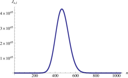
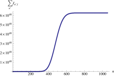
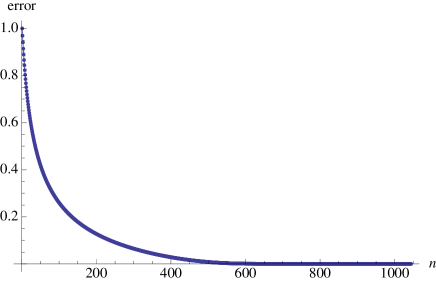
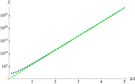
Figure 4: Construction of $f_{\ell}(r,\omega)$ on the PIA using Eq.(12) for $s=2$, $\ell=2$, $r=10M$. Plots (a)–(c) are with $a_{0}=1$, for the value $\bar{\omega}=9.8002i$ and with $n$ on the x-axis. (a) Partial term $J_{n,\ell}$. (b) Partial sum $\sum_{n^{\prime}=0}^{n}J_{n^{\prime},\ell}$. (c) Partial error $\left|J_{n,\ell}/\sum_{n^{\prime}=0}^{n}J_{n^{\prime},\ell}\right|$. (d) Log-plot of $f_{\ell}(r,\omega)$ using Eq.(12) (blue dots interpolated by the continuous blue curve) as a function of $|\bar{\omega}|$ and log-plot of $\left(e^{i\omega r_{*}}+e^{-i\omega r_{*}}\right)$ (dashed green curve), which corresponds to the asymptotics of Eq.(6) ignoring the incidence and reflection coefficients.

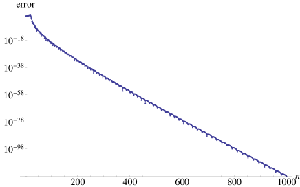
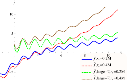
Figure 5: Construction of $\hat{f}_{\ell}$ on the NIA using Eq.(12) for $s=2$, $\ell=2$. (a) Partial error $\left|\hat{J}_{n,\ell}/\sum_{n^{\prime}=0}^{n}\hat{J}_{n^{\prime},\ell}\right|$ as a function of $n$ with $a_{0}=1$ for $\bar{\nu}=9.8002$ and $r=10M$. (b) $\hat{f}_{\ell}$ from Eq.(12) as a function of $\bar{\nu}$. The continuous blue and dotted red curves are calculated using the Jaffé series Eq.(12) for $r_{*}=0.2M$ and $r_{*}=0.4M$ respectively. Note that they are both zero at $\bar{\nu}=\bar{\nu}_{AS}$ because of the fact that, for $s=2$, $\bar{\nu}_{AS}$ is not a pole of $\hat{f}_{\ell}$. The dashed green and dot-dashed brown curves are the large-$\bar{\nu}$ asymptotics in Casals and Ottewill (2012b) for $r_{*}=0.2M$ and $r_{*}=0.4M$ respectively.

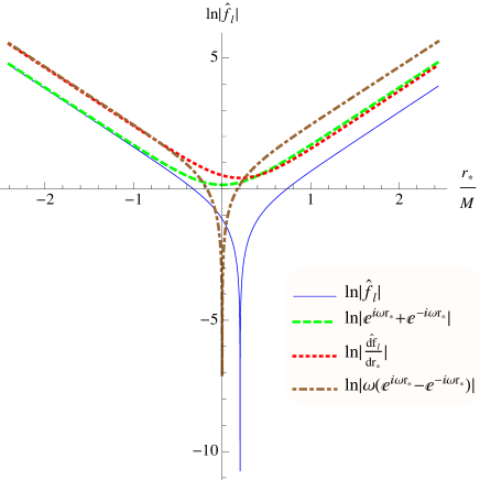
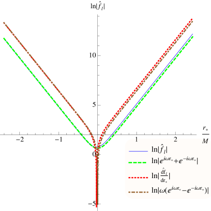
Figure 6: Plots of $\ln|\hat{f}_{\ell}|$ as a function of $r_{*}/M$ for $s=2$, $\ell=2$ and (a) $\bar{\nu}=4.4002$, (b) $\bar{\nu}=9.8002$. Continuous blue curve: $\ln|\hat{f}_{\ell}|$ obtained using Eq.(12). Dashed green curve: $\ln\left|e^{i\omega r_{*}}+e^{-i\omega r_{*}}\right|$. Dotted red curve: $\ln|d\hat{f}_{\ell}/dr_{*}|$ obtained using Eq.(19). Dot-dashed brown curve: $\ln\left|\omega(e^{i\omega r_{*}}+e^{-i\omega r_{*}})\right|$. The curves for $\ln\left|e^{i\omega r_{*}}+e^{-i\omega r_{*}}\right|$ and its radial derivative only serve as very crude approximations to the large-$r$ asymptotics of $\hat{f}_{\ell}$ in Eq.(5).

VI Calculation of $g_{\ell}$ and the BC ‘strength’

VI.1 Recurrence relation

The terms in the series Eq.(13) for $g_{\ell}$, Eq.(17) for $\Delta\tilde{g}_{\ell}$ and Eq.(18) for $\Delta g_{\ell}$ all consist on the coefficient $a_{n}$ times a factor, which we denote by $T_{n}^{(-)}$, $T_{n}^{(0)}$ and $T_{n}^{(+)}$, respectively (times a factor independent of $n$). All three factors, $T_{n}^{(-)}$, $T_{n}^{(0)}$ and $T_{n}^{(+)}$, satisfy the same, following recurrence relation Temme (1983); bk: ; Liu (1997):

$$(n+1-2\bar{\nu})(n-2\bar{\nu})T_{n-1}-(n+1-2\bar{\nu})(2n+1-4\bar{\nu}-2\nu r)T_{n}+(n+1-2\bar{\nu}+s)(n+1-2\bar{\nu}-s)T_{n+1}=0$$ (26)

where $T_{n}$ denotes any of $T_{n}^{(-)}$, $T_{n}^{(0)}$ and $T_{n}^{(+)}$.

In the subsections below we will show the following. On the NIA, all three factors, $T_{n}^{(-)}$, $T_{n}^{(0)}$ and $T_{n}^{(+)}$, have the same leading-order behaviour $O(n^{-1/4}e^{-2i\sqrt{2\nu rn}})$ for large-$n$ – see, respectively, Eqs.(27), (28) and (30) below. The solution $T_{n}^{(-)}$ and either the solution $T_{n}^{(0)}$ or $T_{n}^{(+)}$ of the recurrence relation Eq.(26) are linearly independent . We show that, when solving the recurrence relation (26) for $\omega$ anywhere except on the NIA, $T_{n}^{(-)}$ is a subdominant solution and $T_{n}^{(0)}$ and $T_{n}^{(+)}$ are dominant solutions. In this case of $\omega\notin\text{NIA}$, if one wishes to find $T_{n}^{(-)}$, one expects that forward recurrence will be unstable in that the dominant solution will ‘creep in’ as $n$ is increased. One should then use instead Miller’s algorithm of backward recursion Liu (1997). On the other hand, when solving the recurrence relation (26) on the NIA there are no dominant nor subdominant solutions, all solutions asymptoting like $O(n^{-1/4})$. In this case of $\omega\in\text{NIA}$, there is no danger of a dominant solution ‘creeping in’ and so there is no need for using Miller’s algorithm of backward recursion for finding any of the three solutions.

VI.2 Calculation of $g_{\ell}$

We need a method for calculating the radial solution $g_{\ell}$ on the PIA, as required by $q(\nu)$ in Eq.(11), as well as on the NIA, as required by the Wronskian Eq.(3). We will calculate $g_{\ell}$ directly on the NIA, as well as on the PIA, using the Leaver-$U$ series Eq.(13). As mentioned in Sec. III.2, the Leaver-$U$ series allows us to calculate $g_{\ell}$ directly on the NIA, specifically as the limit from the third quadrant, i.e., $g_{\ell+}$. The advantage of evaluating $g_{\ell}$ on the NIA is twofold. First, no extrapolating procedure $\epsilon\to 0^{+}$ onto the NIA is then needed. Secondly, on the NIA there are no dominant/subdominant solutions to the recurrence relation (26) and so there is no need for Miller’s algorithm of backward recursion.

The confluent hypergeometric $U$-functions, however, are notoriously difficult to evaluate. We have three options in order to calculate the factors $T_{n}^{(-)}$ in the Leaver-$U$ series: (1) from their definition (13) and using the in-built $U$-function in Mathematica, (2) from their definition (13) and using the integral representation Eq.(36) for the $U$-function, and (3) from the above recurrence relation Eq.(26). We note that method (1) is highly unstable, whereas it is a lot more stable to calculate $T_{n}^{(-)}$ using method (2) (see Eq.4.16 Liu (1997), App.B Leung et al. (1999), Temme (1983)).

VI.2.1 Large-$n$ asymptotics

We obtain the large-$n$ behaviour of the terms in the Leaver-$U$ series Eq.(13) in order to investigage its convergence properties. From Eq.(13) and (38), we have

$$T_{n}^{(-)}\sim\frac{e^{-\nu r}}{\Gamma(1-2\bar{\nu})(2|\nu|r)^{s}}\sqrt{\frac{\pi}{\sqrt{2|\nu|r}}}e^{-i\chi(s+1/4)}n^{-1/4}e^{-2\sqrt{2|\nu|rn}e^{i\chi/2}},\quad n\to\infty,\quad s\leq 0,\ \chi\equiv\arg(-\nu)\in(-\pi,+\pi],\ r>0$$ (27)

agreeing with Eq.4.19 Liu (1997). It follows from Eq.(27) that the series for $\tilde{h}_{n,\ell}$ is absolutely convergent everywhere except, maybe, on the NIA.

The convergence properties of the series $h_{\ell}=\sum_{n}h_{n,\ell}$ on the NIA (which would yield $g_{\ell+}$) is the same as that for $\Delta\tilde{h}_{\ell}=\sum_{n}\Delta\tilde{h}_{n,\ell}$ in Sec.VI.3.2 and as that for $\Delta h_{\ell}=\sum_{n}\Delta h_{n,\ell}$ in Sec.VI.4.1, and so we refer the reader to this latter section.

VI.2.2 Results

In Fig.7 we plot $g_{\ell+}$ as a function of the frequency on the NIA. Since $g_{\ell}\to e^{\nu r}\in\mathbb{R}$ for large $r$ and the asymptotic series for $g_{\ell}$ for large $r$ contains only real coefficients (e.g., Sec.B.1 Liu (1997)), one would expect that $|\text{Im}(g_{\ell+})|\ll|\text{Re}(g_{\ell+})|$, especially as $\bar{\nu}$ increases - this is indeed what happens in Fig.7. Fig.7 shows that $\text{Im}(g_{\ell+})$ becomes round-off error at some stage . In Fig.2 Casals and Ottewill (2012b) we show similar plots for $s=0$.

When calculating the terms in the series Eq.(13) for $g_{\ell+}(r,-i\nu)$ in practise using Mathematica, the first two terms $T_{n=0}^{(-)}$ and $T_{n=1}^{(-)}$ on the NIA we calculate using Eq.(36) and a particular splitting of some expression for the $U$-function instead of obtaining it using Mathematica’s in-built HypergeometricU function.

In Fig.8 we plot both the radial function $g_{\ell+}$ and its radial derivative as functions of the radius. The radial derivative as a function of the frequency has a very similar behaviour to that of $g_{\ell+}$ in Fig.7.

On the PIA, as noted in Sec.VI.2.1, solving the recurrence relation Eq.(26) to obtain $g_{\ell}$ is unstable since it corresponds to the subdominant solution and the dominant solution would be ‘creeping in’. One option is to obtain $g_{\ell}(r,+i\nu)$ using Eqs.(13) and (38). In Fig.9 we show that using the recurrence relation is unstable whereas the latter option does well. The following is the method we follow: when calculating the terms in the series Eq.(13) for $g_{\ell}(r,+i\nu)$ in practise in Mathematica, we use a numerical evaluation of the integral representation Eq.(36) in order to calculate $T_{n}^{(-)}$, $\forall n$, on the PIA instead of obtaining it by solving the recurrence relation that it satisfies.

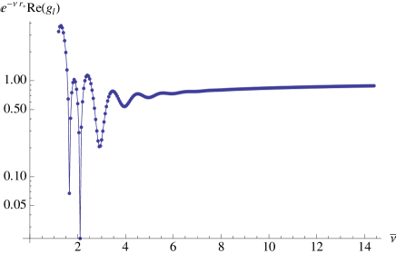
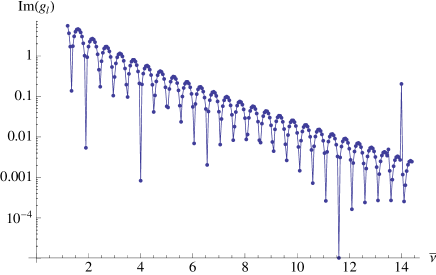
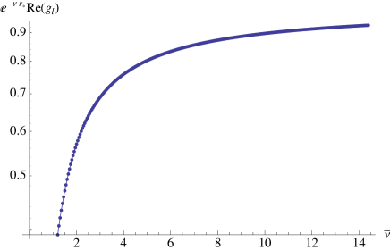
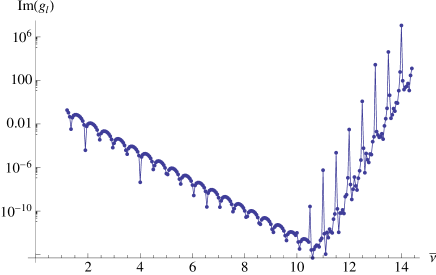
Figure 7: Log-plots of the radial solution $g_{\ell+}$ as a function of $\bar{\nu}$ for $s=2$, $\ell=2$. Top plots (a) and (b) are for $r=2.8M$ and bottom plots (c) and (d) are for $r=5M$. Left plots (a) and (c) are $e^{-\nu r_{*}}\text{Re}(g_{\ell+})$ and right plots (b) and (d) are $\text{Im}(g_{\ell+})$, all obtained using Eq.(13) and finding $T_{n}^{(-)}$ by solving the recurrence relation (26) with $T_{0}^{(-)}$ and $T_{1}^{(-)}$ calculated using Mathematica’s in-built HypergeometricU function. Cf. Fig.2 Casals and Ottewill (2012b). A similar behaviour is exhibited by the radial derivative $dg_{\ell+}/dr_{*}$.

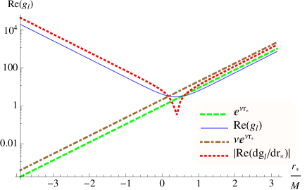
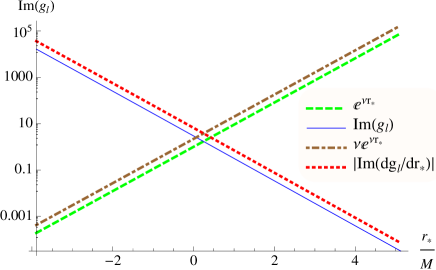
Figure 8: Log-plots of $g_{\ell+}$ and $dg_{\ell+}/dr_{*}$ as functions of $r_{*}/M$ for $s=2$, $\ell=2$, $\bar{\nu}=4.4002$. These radial functions are obtained using Eqs.(13) and (20) and finding $T_{n}^{(-)}$ by solving the recurrence relation (26) with $T_{0}^{(-)}$ and $T_{1}^{(-)}$ calculated using Mathematica’s in-built HypergeometricU function. (a) Continuous blue curve: $\text{Re}(g_{\ell})$; dashed green curve: large-$r$ asymptotics $g_{\ell}\sim e^{\nu r_{*}}$; dotted red curve: $\left|\text{Re}(dg_{\ell+}/dr_{*})\right|$; dot-dashed brown curve: large-$r$ asymptotics $dg_{\ell+}/dr_{*}\sim\nu e^{\nu r_{*}}$. (b) Similar as (a) but the continuous blue curve and the dotted red curve here correspond to the imaginary – instead of real – part of $g_{\ell+}$ and $dg_{\ell+}/dr_{*}$ respectively. We note that for $\bar{\nu}=9.8002$ the calculation of the imaginary part using the method as in these plots becomes unstable for $r_{*}\gtrapprox 8M$.

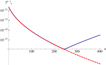
Figure 9: Radial solution $g_{\ell}$ on the PIA for $s=2$, $\ell=2$, $r=5M$. (a) Continuous blue curve: $T_{n}^{(-)}$ in Eq.(13) as a function of $n$ for $\bar{\omega}=4.4002i$ obtained using Mathematica’s HypergeometricU function (a similar curve is obtained by solving the recurrence relation Eq.(26)); this curve shows how the dominant solution ‘creeps in’ in the solution of the recurrence relation. Dashed red curve: similar to the continuous blue curve but $T_{n}^{(-)}$ is obtained using Eq.(36). (b) $g_{\ell}(r,+i\nu)$ as a function of $|\bar{\omega}|$ on the PIA obtained by numerically evaluation the numerical representation Eq.(36): convergence is achieved up to large values of $|\bar{\omega}|$ whereas using the recurrence relation Eq.(26) the series coincides with the curve plotted up to $|\bar{\omega}|\approx 14$ but ceases to converge after that value.

VI.3 Calculation of $\Delta\tilde{g}_{\ell}$

From Eq.13.4.15 Abramowitz and Stegun (1972) and the property $\Gamma(z+1)=z\Gamma(z)$ we easily see that $T_{n}^{(0)}$ satisfy the recurrence relation Eq.(26). In Fig. 10 we plot $e^{13M\nu}\Delta\tilde{g}_{\ell}(r,\nu)$ as a function of $\bar{\nu}$ obtained with Eq.(17). Note that, when carried out in practise in Mathematica, it is better to numerically evaluate the integration representation Eq.(36) instead of using Mathematica’s in-built HypergeometricU function in order to calculate the two initial values $T_{n=0}^{(0)}$ and $T_{n=1}^{(0)}$.

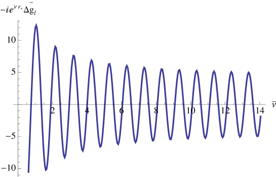
Figure 10: Plot of ‘$-ie^{\nu r_{*}}\Delta\tilde{g}_{\ell}$’ as a function of $\bar{\nu}$ for $s=2$, $\ell=2$, $r=10M$. We have obtained $\Delta\tilde{g}_{\ell}$ from Eq.(17) by solving the recurrence relation Eq.(26) with $T_{0}^{(0)}$ and $T_{1}^{(0)}$ calculated using Mathematica’s in-built HypergeometricU function. We have removed from $\Delta\tilde{g}_{\ell}$ the large-$r$ behaviour of Eq.(11): $g_{\ell}(r,+i\nu)\sim e^{-\nu r_{*}}$. The zeros of the curve occur at $\bar{\nu}$-steps of approximately $1/2$, agreeing with the large-$\bar{\nu}$ asymptotics of $q(\nu)$ in Eq.38 Casals and Ottewill (2012b).

VI.3.1 Zeros and singularities of $\Delta\tilde{h}_{n,\ell}$

Any possible zeros and singularities of the terms $\Delta\tilde{h}_{n,\ell}$ in Eq.(17) may only come from the $\tilde{a}_{n}$, the $U$-function and the four $\Gamma$-functions. The $U$-function has no singularities other than its branch point, and the $\Gamma$-function has no zeros. We do not know analytically the possible zeros of $\tilde{a}_{n}$ nor of the $U$-function, so we can only determine some of the zeros of $\Delta\tilde{h}_{n,\ell}$, and we cannot be sure that any of the poles we might find are not actually cancelled out by zeros of $\tilde{a}_{n}$ and/or the $U$-function.

From Sec.IV.1 we know that $a_{n}$ have simple poles $\forall n\geq k$ if $\bar{\nu}=k/2$ for some $k\in\mathbb{N}$ (with the exception of $\nu=\nu_{AS}$ when $s=2$). The function $\Gamma(z)$ has simple poles at $z\in\mathbb{Z}^{-}$. Let us distinguish two cases:

• Case $1-2\bar{\nu}\notin\mathbb{Z}^{-}\cup{0}$

  Neither $a_{n}$ nor the $\Gamma$-functions have any pole. So $\Delta\tilde{h}_{n,\ell}$ has no zeros (other than any coming from $a_{n}$ or the $U$-function) and it has no poles.

• $1-2\bar{\nu}\equiv-k\in\mathbb{Z}^{-}\cup{0}$

  In the numerator, $a_{n}$ has simple poles (except if $\nu=\nu_{AS}$ when $s=2$) at $n=k,k+1,k+2,\dots$ and $\Gamma(1+n-2\bar{\nu})$ at $n=0,1,2,\dots,k$. In the denominator, $\Gamma(1+s+n-2\bar{\nu})\Gamma(1-s+n-2\bar{\nu})$ has double poles at $n=0,1,2,\dots,k-|s|$ and simple poles at $n=k-|s|+1,k-|s|+2,\dots,k+|s|$. Also in the denominator, $\Gamma(1-2\bar{\nu})$ has a simple pole $\forall n\in\mathbb{N}$. Therefore, $\Delta\tilde{h}_{n,\ell}$ has no poles. Regarding the zeros (other than any coming from $a_{n}$ or the $U$-function), if $n\neq k$, $\Delta\tilde{h}_{n,\ell}$ has double zeros at $n=0,1,2,\dots,k-|s|$ and simple zeros at $n=k-|s|+1,k-|s|+2,\dots,k+|s|$; the term $n=k$ is not a zero if $s\neq 0$ and it is just a simple zero if $s=0$.

  In the particular case $\nu=\nu_{AS}$ for $s=2$, $a_{n}$ does not have a pole for any $n\in\mathbb{N}$. In this case, a similar analysis to the one in the above paragraph indicates that $\Delta\tilde{h}_{n,\ell}$ has a zero there. .

VI.3.2 Large-$n$ asymptotics

Using Eq.(37) and Eq.5.11.3 bk: we obtain

$$T_{n}^{(0)}\sim\frac{e^{\nu r}(2\nu r)^{-s-1/4}}{\sqrt{\pi}}(-1)^{n}n^{-1/4}\cos\left(\sqrt{4\nu r\left(2n-4\bar{\nu}+1\right)+\pi\left(2\bar{\nu}-n-\frac{1}{4}\right)}\right),\quad n\to\infty,\quad\text{if }s\geq 0\ \text{and}\ \nu r>0$$ (28)

Finally, together with the large-$n$ asymptotics (24) for $a_{n}$ we can obtain the large-$n$ asymptotics of the terms in the series for $\Delta\tilde{h}_{\ell}$:

$$\Delta\tilde{h}_{n,\ell}\sim\tilde{C}(\nu,r)(-1)^{n}n^{-\bar{\nu}-1}e^{\pm 2\sqrt{2n\bar{\nu}}i}\cos\left(\sqrt{4\nu r\left(2n-4\bar{\nu}+1\right)+\pi\left(2\bar{\nu}-n-\frac{1}{4}\right)}\right),\quad n\to\infty,\quad\text{if }s\geq 0\ \text{and}\ \nu r>0$$ (29)

$$\tilde{C}(\nu,r)\equiv\frac{2\sqrt{\pi}ie^{-\nu r}e^{\pi i(s+1-2\bar{\nu})}(-2\bar{\nu})^{s+1-2\bar{\nu}}(2\nu r)^{-s-1/4}}{\Gamma(1-2\bar{\nu})}$$

for fixed $\nu$. The modulus of the large-$n$ asymptotics of $\Delta\tilde{h}_{n,\ell}$ in Eq.(29) is basically the same as that for $\Delta h_{n,\ell}$ in Eq.(31) below. Therefore the conclusions below Eq.(31) regarding the convergence of the series $\Delta h_{\ell}=\sum_{n}\Delta h_{n,\ell}$ apply equally to the series $\Delta\tilde{h}_{\ell}=\sum_{n}\Delta\tilde{h}_{n,\ell}$.

VI.4 Calculation of $\Delta g_{\ell}$

From Eq.13.4.1 Abramowitz and Stegun (1972) and the property $\Gamma(z+1)=z\Gamma(z)$ we easily find that the $T_{n}^{(+)}$ satisfy the same recurrence relation Eq.(26) as the $T_{n}^{(-)}$ in the series for $g_{\ell}$ and the $T_{n}^{(0)}$ in the series for $\Delta\tilde{g}_{\ell}$ – see Liu (1997); Temme (1983). To investigate the convergence properties of this series, we require the large-$n$ asymptotics of its terms.

VI.4.1 Large-$n$ asymptotics

From Eqs.13.1.27 and 13.5.14 Abramowitz and Stegun (1972) we obtain

$$T_{n}^{(+)}\sim\pi^{-1/2}e^{-\nu r}\Gamma(2s+1)\left(2\nu r\right)^{-1/4-s}n^{-1/4}\cos\left(\sqrt{\left(1-4\bar{\nu}+2n\right)4\nu r}-\frac{\pi(4s+1)}{4}\right),\quad n\to\infty,$$ (30)

which is valid for $(n-2\bar{\nu}-s)\to+\infty$, $s$ bounded and $\nu r\in\mathbb{R}$. This agrees with Eq.4.20 Liu (1997) (except for a typo they have in the sign of $s$ inside the $\Gamma$-function ). [Note: Eq.(30) differs from Eq.12 in Sec.6.13.2 of Erdelyi et al. (1953) in having an extra factor $1/2$ and also a power ‘$-1/4-s$’ instead of a ‘$+1/4-s$’. We have, however, checked with Mathematica for certain values of the parameters that Eq.(30) is the correct expression.]

From Eq.(30) and the large-$n$ asymptotics (24) for $a_{n}$ we can now obtain the large-$n$ asymptotics of the terms in the series for $\Delta g_{\ell}$:

$$\Delta h_{n,\ell}\sim C(\nu,r)\left(n-2\bar{\nu}+\frac{1}{2}\right)^{-\bar{\nu}-1}e^{\pm 2\sqrt{-2n\bar{\nu}}}\cos\left(\frac{\pi(4s+1)}{4}-2\sqrt{\left(n-2\bar{\nu}+\frac{1}{2}\right)2\nu r}\right),\quad n-2\bar{\nu}\gg 1,$$ (31)

$$C(\nu,r)\equiv\frac{(-1)^{2s}2\sqrt{\pi}i\left(2\nu r\right)^{-1/4-s}e^{-\nu r}}{\Gamma(1-2\bar{\nu})}$$

The ratio test yields $\left|\Delta h_{n+1,\ell}/\Delta h_{n,\ell}\right|\to 1$ as $n\to\infty$, and so it is inconclusive. However, we may apply the integral test as follows. For $\bar{\nu}>0$, the function $k(n)\equiv\left|C(\nu,r)\right|n^{-\bar{\nu}-1}=|k(n)|$ is positive and monotone decreasing with $n$ and it satisfies

$$\int_{1}^{\infty}dn|k(n)|=\left|C(\nu,r)\right|\int_{1}^{\infty}dn\ n^{-\bar{\nu}-1}=\frac{\left|C(\nu,r)\right|}{\bar{\nu}}\left[1-\lim_{n\to\infty}n^{-\bar{\nu}}\right]<\infty,\qquad\text{if}\quad\bar{\nu}>0.$$ (32)

Therefore $|k(n)|$ satisfies the integral test and so the series $\sum_{n}k(n)$ is absolutely convergent for $\bar{\nu}>0$. Since $\left|\Delta h_{n,\ell}\right|<|k(n)|$ for sufficiently large $n$, from the comparison test we have that $\sum_{n}\Delta h_{n,\ell}$ is also absolutely convergent for $\bar{\nu}>0$. Indeed, in our calculations, the series has converged for arbitrary values of $\bar{\nu}$. However, while the series is fast convergent for large $\bar{\nu}$ the speed of convergence becomes slower for smaller values $\bar{\nu}$.

VI.5 Calculation of $q(\nu)$

We calculate the BC ‘strength’ $q(\nu)$ using Eq.(11), where we calculate $\Delta\tilde{g}_{\ell}$ using the method described in Sec.VI.3 and $g_{\ell}(r,+i\nu)$ on the PIA using Eq.(13) with $\nu\to-\nu$ everywhere. We note that an alternative method, which we have not explored, for calculating $g_{\ell}(r,+i\nu)$ might be to use Eq.74 Leaver (1986b). In Fig. 11 we plot $q(\nu)$ as a function of $\bar{\nu}$. This figure is to be compared with Fig.2 Leung et al. (2003a) (also Fig.2. Leung et al. (2003b)).

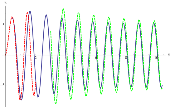
Figure 11: BC ‘strength’ $q(\nu)$ of Eq.(11) as a function of $\bar{\nu}$ for $s=2$, $\ell=2$. Continuous blue curve: $q(\nu)$ obtained using Eq.(11) with the value $r=5M$ and $g_{\ell}(r,+i\nu)$ obtained using Eq.(36). Dashed green curve: large-$\bar{\nu}$ asymptotics of Eq.38 Casals and Ottewill (2012b) (see Fig.5 Casals and Ottewill (2012b) for a better agreement for larger values of $\bar{\nu}$). Dot-dashed red curve: small-$\bar{\nu}$ asymptotics of Eqs.2.2 and 2.5 Leung et al. (2003a) (we note that the small-$\bar{\nu}$ asymptotics in Leung et al. (2003a) do not work well for other spins; see Casals and Ottewill for better agreement for small-$\bar{\nu}$ for any spin). Cf. Fig.2 Leung et al. (2003a) (also Fig.2. Leung et al. (2003b)). We note that when $g_{\ell}(r,+i\nu)$ is obtained using the recurrence relation Eq.(26) instead of Eq.(36), the result for $q(\nu)$ is incorrect from $\bar{\nu}\approx 11$ - see Fig.9(a).

VII Calculation of the Wronskian

We calculate, on the NIA, the Wronskian $\hat{W}_{+}$ of the radial solutions $\hat{f}_{\ell}\equiv-\sin(2\pi i\bar{\omega})f_{\ell}$ and $g_{\ell+}$ using the methods described in the previous sections: the Jaffé series Eq.(12) for $f_{\ell}$, Eq.(19) for $df_{\ell}/dr_{*}$, the Leaver-$U$ series Eq.(13) for $g_{\ell+}$ and Eq.(20) for $dg_{\ell+}/dr_{*}$.

In Figs.5–8 we plot, on the NIA, the radial solutions $\hat{f}_{\ell}(r,-i\nu)$ and $g_{\ell+}(r,-i\nu)$ and their radial derivatives, which are required for the Wronskian.

Let us define $\hat{W}_{1}\equiv g_{\ell+}\hat{f}_{\ell}^{\prime}$ and $W_{2}\equiv\hat{f}_{\ell}g_{\ell+}^{\prime}$, so that $\hat{W}_{+}=\hat{W}_{1}-\hat{W}_{2}$. Figs.12(a) and (b) show that the magnitudes of the two contributions $\hat{W}_{1}$ and $\hat{W}_{2}$ are very close for all $r_{*}$ except near $r_{*}=0$. Therefore, the computation of $\hat{W}=\hat{W}_{1}-\hat{W}_{2}$ would require the knowledge of these two contributions to very high accuracy away from this ‘window’ near $r_{*}=0$. We note that for the imaginary part, for $r_{*}\geq 0$ the two contributions $\hat{W}_{1}$ and $\hat{W}_{2}$ actually add up and so there is no computational difficulty there either. Figs.12(c) shows that, indeed, there is a ‘window’ near $r_{*}=0$ where the calculation of the absolute value of the Wronskian is reliable. We note that in this ‘window’ it is $\text{Im}(\hat{W})\gg\text{Re}(\hat{W})$, so the imaginary part dominates but, for accuracy, the real part cannot be neglected. We have checked that a similar ‘window’ near $r_{*}=0$ occurs for different values of the spin, the multipole number $\ell$ and the frequency on the NIA.

In Figs.13 we plot $\hat{W}_{1}$, $\hat{W}_{2}$ and $\hat{W}$ at $r=2.8M$ as functions of $\bar{\nu}$. Fig.13(c), together with Figs.7–9 Casals and Ottewill (2012b) where these ‘mid’-frequency results are compared to large-$\bar{\nu}$ asymptotics, show that the calculation of the Wronskian at this value of the radius yields a reliable result. In Casals and Ottewill we show that the ‘mid’-frequency results for the Wronskian agree well with small-$\bar{\nu}$ asymptotics. Fig.13(c) also shows – for the particular value $\ell=2$ – that for $s=2$ the Wronskian $\hat{W}_{+}\equiv W[g_{\ell+},\hat{f}_{\ell}]$ has a zero of order one at $\nu=\nu_{AS}$. This is as expected because of the definition $\hat{f}_{\ell}\equiv-\sin(2\pi i\bar{\omega})f_{\ell}$ and the fact that $\bar{\nu}=\bar{\nu}_{AS}$ is not a pole of $f_{\ell}$ for $s=2$ and it agrees with  Leung et al. (2003a).

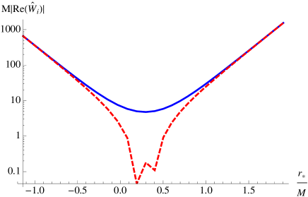
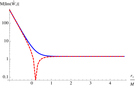
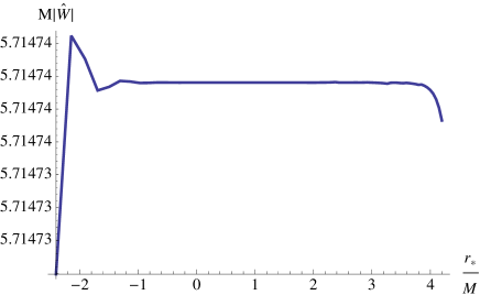
Figure 12: Wronskian $\hat{W}_{+}\equiv W[g_{\ell+},\hat{f}_{\ell};\omega]=\hat{W}_{1}-\hat{W}_{2}$ as a function of $r_{*}/M$ for $s=2$, $\ell=2$ and $\bar{\nu}=4.4002$. Figs.(a) and (b): log-plots of the absolute values of, respectively, the real and imaginary parts of $M\cdot\hat{W}_{1}\equiv Mg_{\ell+}\hat{f}_{\ell}^{\prime}$ (continuous blue curve) and $M\cdot\hat{W}_{2}\equiv M\hat{f}_{\ell}g_{\ell+}^{\prime}$ (dashed red curve). Fig.(c): Log-plot of $M|\hat{W}|$.

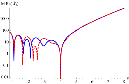
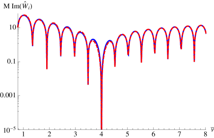
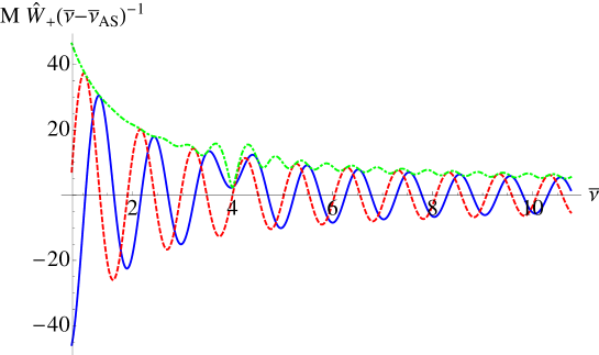
Figure 13: Wronskian $\hat{W}\equiv W[g_{\ell},\hat{f}_{\ell};\omega]=\hat{W}_{1}-\hat{W}_{2}$ as a function of $\bar{\nu}$ for $s=2$, $\ell=2$, $r=2.8M$ ($r_{*}\approx 0.97M$). (a) and (b): log-plots of, respectively, the real and imaginary parts of both $M\hat{W}_{1}$ (continuous blue curve) and $M\hat{W}_{2}$ (dashed red curve). (c) Plot of the real part (continuous blue curve), imaginary part (dashed red curve) and absolute value (dot-dashed green curve) of $M\hat{W}_{+}/(\bar{\nu}-\bar{\nu}_{AS})$. We note the zero of order one of $|\hat{W}_{+}|$ at the algebraically special frequency $\bar{\nu}=\bar{\nu}_{AS}$.

VIII Calculation of BC modes

We obtain the branch cut modes $\Delta G_{\ell}(r,r^{\prime};\nu)$ by calculating the different quantities in Eq.(10) using the methods described in the previous sections. In particular, for the calculation of the Wronskian we have evaluated the radial functions $\hat{f}_{\ell}$ and $g_{\ell}$ at $r=2.8M$ while for the branch cut ‘strength’ $q(\nu)$ we have evaluated the radial functions at $r=5M$. In Fig.14 we plot $\Delta G_{\ell}$ as a function of $\bar{\nu}$ for different spins. In the spin-2 case the plot is to be compared with Fig.3 Leung et al. (2003a) (also Fig.3 Leung et al. (2003b)). From Figs.5, 11, 13(c) respectively, the radial solution $\hat{f}_{\ell}$, the BC ‘strength’ $q$ and the absolute value of the Wronskian $|\hat{W}|$ all have a simple zero at $\bar{\nu}=\bar{\nu}_{AS}$ in the case $\nu=\nu_{AS}$ and $s=\ell=2$. From Eq.(10) it then follows that $\Delta G_{\ell}$ has a simple zero at that frequency, as Fig.14(c) reflects. In Fig.15 we plot again $\Delta G_{\ell}(r,r^{\prime};\nu)$ but in this case for larger values of the radius $r^{\prime}$: the magnitude of $\Delta G_{\ell}$ increases rapidly with the radius, as expected from Fig.5(b).

The spin-$2$ case is quite distinct due to the algebraically special frequency $\bar{\nu}_{AS}$ ($=4$ when $\ell=2$): while the branch cut mode $\Delta G_{\ell}$ is zero at $\bar{\nu}=\bar{\nu}_{AS}$, $\Delta G_{\ell}$ is particularly large for frequencies near $\nu_{AS}$. This behaviour is explained, in the case $\ell=2$ and $r^{\prime}_{*}\to-\infty$ and $r_{*}\to\infty$, as arising from nearby ‘unconventional damped modes’, that is a pair of poles in the unphysical Riemann sheet. The imaginary part of the QNM frequencies is negative and increases in magnitude as the overtone number $n$ increases, so that $n$ is an index for the speed of damping of the mode with time. For spin-2, QNM frequencies approach the algebraically special frequency as $n$ is increased from the lowest damped mode, $n=0$, until a certain value of $n$, say $n_{M}$, whose QNM frequency is very close to $\bar{\omega}_{AS}$; for $\ell=2$ it is $n_{M}=9$. As $n$ is further increased from $n_{M}$, the real part of the spin-2 QNM frequencies in the 3rd quadrant increases monotonically. Therefore, in a certain sense, the algebraically special frequency marks the start of the highly-damped asymptotic regime for QNMs.

In Fig.16 we plot the radius-independent quantity ‘$|2\nu q/(M\hat{W}^{2})|$’, which is the branch cut mode $\Delta G_{\ell}$ of Eq.(10) but without the $f_{\ell}$ factors. The zeros of this radius-independent quantity correspond to the zeros of $q(\nu)$. Fig.16 shows that, for the cases with $s=1$ and $2$, these zeros occur with a period in $\bar{\nu}$ close to that of the increment in the imaginary part of the QNM frequencies $\bar{\omega}_{QNM}$ at consecutive overtone numbers. For $s=2$, (minus) the imaginary part of the QNM frequencies lie close to the zeros of $q(\nu)$. For $s=1$, for which the QNM frequencies approach the NIA particularly fast Casals and Ottewill (2012b), (minus) the imaginary part of the QNM frequencies lie close to the maxima points of ‘$|2\nu q/(M\hat{W}^{2})|$’ which are directly related to nearby zeros of $\hat{W}$, i.e., the QNM frequencies by definition. For $s=0$, on the other hand, the periods of the zeros of $q(\nu)$ and of $\text{Im}(\bar{\omega}_{QNM})$ differ slightly for mid-$\bar{\nu}$ while, for large-$\bar{\nu}$, ‘$-\text{Im}(\bar{\omega}_{QNM})$’ tend to lie somewhere in-between the zeros of $q(\nu)$ and the maxima points of ‘$|2\nu q/(M\hat{W}^{2})|$’. For all spins in the large-$\bar{\nu}$ asymptotic regime, the separation of the zeros of $q(\nu)$ approaches $1/2$, which coincides with the separation in the imaginary part of highly-damped QNM frequencies for consecutive overtone numbers (see, e.g., Casals and Ottewill (2012b) for the asymptotic expressions).

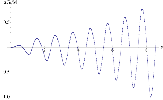
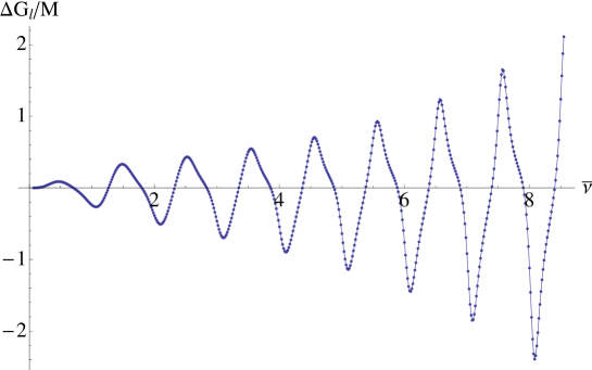
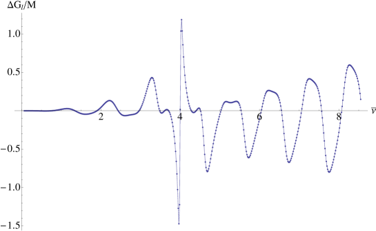
Figure 14: Branch cut mode $\Delta G_{\ell}/M$ of Eq.(10) as a function of $\bar{\nu}$ for $r_{*}=0.2M$ and $r^{\prime}_{*}=0.4M$. The Wronskian has been calculated at $r=2.8M$ while $q(\nu)$ has been calculated with functions at $r=5M$. (a) $s=0$, $\ell=1$. (b) $s=1$, $\ell=1$. (c) $s=2$, $\ell=2$ – cf. Fig.3 Leung et al. (2003a) (also Fig.3 Leung et al. (2003b)).

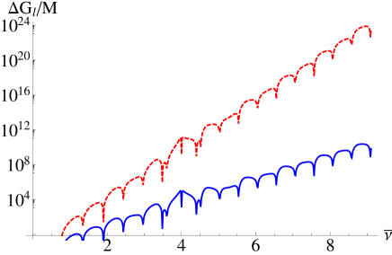
Figure 15: Same as Fig.14(c), i.e., $\Delta G_{\ell}/M$ as a function of $\bar{\nu}$ for $s=2$, $\ell=2$ and $r_{*}=0.2M$ but here it is with $r^{\prime}_{*}=r_{*}(r=5M)$ in the continuous blue curve and $r^{\prime}_{*}=r_{*}(r=10M)$ in the dashed red curve.

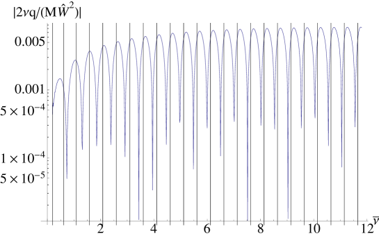
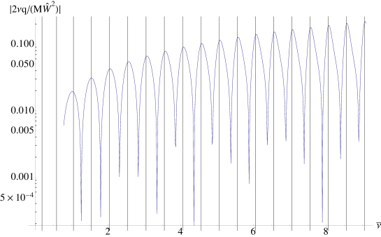
Figure 16: Log-plot of ‘$|2\nu q/(M\hat{W}^{2})|$’ (this is the branch cut mode $\Delta G_{\ell}$ of Eq.(10) but without the $\hat{f}_{\ell}$ factors) as a function of $\bar{\nu}$. The vertical lines are located at the values of (minus) the imaginary part of the QNM frequencies – obtained from QNM for the cases $s=1$ and $s=2$ and using Dolan and Ottewill for $s=0$. The Wronskian $\hat{W}$ and the BC ‘strength’ $q(\nu)$ have been calculated by evaluating the radial solutions at, respectively, $r=2.8M$ and $r=5M$. (a) $s=0$, $\ell=1$. (b) $s=1$, $\ell=1$. (c) $s=2$, $\ell=2$: in this case we log-plot ‘$|2\nu q(\bar{\nu}-\bar{\nu}_{AS})^{2}M/\hat{W}^{2}|$’, i.e, we include an extra factor $|\bar{\nu}-\bar{\nu}_{AS}|^{2}$ to account for the double zero of $|\hat{W}|^{2}$ at $\bar{\nu}=\bar{\nu}_{AS}$).

IX Self-force

The motion of a (non-test) point particle moving on a background space-time deviates from geodesic motion of that space-time due to a self-force (see, e.g., Poisson et al. (2011) for a review). The self-force may be calculated via an integration of the covariant derivative of the retarded Green function integrated over the whole past worldline of the particle. In particular, for a scalar charge $q$ moving on Schwarzschild background space-time, the $\mu$-component of the self-force is given by

$$f_{\mu}(\tau)=q\int_{-\infty}^{\tau^{-}}d\tau^{\prime}\ \nabla_{\mu}G_{ret}(z(\tau),z(\tau^{\prime}))$$ (33)

where $z(\tau)$ is the worldline of the particle and $\tau$ is its proper time. In the rest of this section we will deal with the case of a scalar charge ($s=0$) only, although the self-force in the cases of an electromagnetic charge ($s=1$) and of a point mass ($s=2$) also involve the integration of the Green function in a similar way. We will investigate the contribution to the scalar self-force from a single BC multipole mode $G_{\ell}^{BC}(r,r^{\prime};t)$ in the case of a particle on a worldline at constant radius. .

In Fig.17 we construct the mode $\ell=1$ of the retarded Green function, $G^{ret}_{\ell}(r,r^{\prime};t)$, in the scalar case $s=0$ at the radii $r=r^{\prime}=10M$. We plot: (1) the BC contribution to $G^{ret}_{\ell}$, i.e., $G_{\ell}^{BC}$, (2) the sum of $G_{\ell}^{BC}$ and the QNM contribution to $G^{ret}_{\ell}$ (taking into account the QNMs for the first 24 overtones), and (3) the full ‘exact’ $G^{ret}_{\ell}$. We calculate $G_{\ell}^{BC}$ by integrating over the frequency the BC modes $\Delta G_{\ell}$ obtained using two different methods in the ‘mid’-frequency and large-frequency regimes - in this case, the crossover frequency is at $\bar{\nu}=50$ . In the ‘mid’-frequency regime, we interpolate the values of the BC modes $\Delta G_{\ell}$ obtained as described in the previous section. In the large-frequency regime we use the asymptotics of Casals and Ottewill (2012b) for the BC modes. We calculate the QNM contribution to $G^{ret}_{\ell}$ using the method in Dolan and Ottewill . We obtain the ‘exact’ $G^{ret}_{\ell}$ by numerically integrating the (1+1)-dimensional partial differential equation $\left(-\partial^{2}_{t}+\partial^{2}_{r_{*}}-V\right)\phi_{\ell}(r,t)=0$ (with the potential $V$ given by Eq.(4)) for the $\ell$-mode $\phi_{\ell}$ of the field using the following initial data. We choose zero data for the inital value of the $\ell$-mode of the field. For the initial value of the time-derivative of the $\ell$-mode of the field, on the other hand, we choose a Gaussian distribution in $r_{*}$ ‘peaked’ at a certain value $r_{*0}$. From the Kirchhoff integral representation for the field (e.g., Leaver (1986a)), the solution $\phi_{\ell}(r,t)$ thus obtained should approximate the $\ell$-mode of the retarded Green function, $G^{ret}_{\ell}(r,r_{0};t)$, where $r_{0}\equiv r(r_{*0})$ . We used a Gaussian width of approximately $0.2M$ and we checked that the change in the numerical solution obtained by using smaller values of the width was negligible for our purposes. For the numerical integration of the (1+1)-dimensional partial differential equation we used Wardell’s C-code available in Wardell . A slightly different version of this numerical approach using a Gaussian distribution (though using it as the source, rather than as initial data) has recently been successfully applied in Zenginoglu and Galley (2012) in the full (3+1)-dimensional case. We observe from Fig.17 that the BC contribution becomes most significant for small values of the ‘time’ $T\equiv t-|r_{*}|-|r^{\prime}_{*}|$ but, in the regime plotted, the BC contribution is always subdominant to the QNM contribution. The matching between the numerical solution and the sum of $G_{\ell}^{BC}$ plus QNM series is excellent. For $T<0$ neither the QNM series nor the BC integral is expected to converge separately Casals and Ottewill (2012b).

Let us now define the ‘$\ell$-mode of the partial field’ as

$$\phi_{\ell}^{partial}(r)\equiv\int_{2|r_{*}|}^{\infty}dt\ G^{ret}_{\ell}(r,r^{\prime}=r;t)$$ (34)

The contribution to the radial component of the self-force per unit charge in the case of a particle at constant radius from the $\ell$-mode of the Green function from the segment of the worldline lying between $t=2|r_{*}|$ and $t\to\infty$ is then obtained as:

$$\frac{f_{\ell,r}^{partial}(r)}{q}\equiv\frac{(2\ell+1)}{r^{2}}P_{\ell}(\cos\gamma)\frac{d\tau}{dt}\left[\frac{d\phi_{\ell}^{partial}}{dr}-\frac{\phi_{\ell}^{partial}}{r}\right]$$ (35)

This clearly only yields a partial contribution to the self-force from the $\ell$-mode since we are integrating from $t=2|r_{*}|$ instead of from $t=0^{+}$, as required in order to obtain the self-force. Because of the divergence of the BC and QNM contributions for $T<0$, in order to obtain the contribution from the worldline segment for $t:0^{+}\to 2|r_{*}|$ we require a different method for calculating the Green function, such as a quasi-local series (see, e.g., Casals et al. (2009a)). The BC contribution to $\phi_{\ell}^{partial}$ is obtained by inserting $G_{\ell}^{BC}$ in the place of $G^{ret}_{\ell}$ in Eq.(34). In Fig.18(a) we plot this contribution and its $r_{*}$-derivative (evaluated using a central difference scheme) as functions of the radius in the case $s=0$ and $\ell=1$. In Fig.18(b) we plot the corresponding BC contribution to $f_{\ell,r}^{partial}(r)/q$ in the static case $\gamma=0$ and $d\tau/dt=(1-2M/r)^{1/2}$.

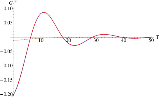
Figure 17: Mode $\ell=1$ of the retarded Green function, i.e., $G^{ret}_{\ell}(r,r^{\prime};t)$, for $s=0$ and $r=r^{\prime}=10M$ as a function of the ‘time’ $T\equiv t-|r_{*}|-|r^{\prime}_{*}|$. Continuous blue curve: ‘exact’ numerical solution $G^{ret}_{\ell}$ obtained using Wardell . Dashed black curve: $G_{\ell}^{BC}$ of Eq.(9). Dot-dashed red curve (overlapping with the continuous blue curve): $G_{\ell}^{BC}$ plus the corresponding QNM series contribution (summing overtone numbers $n:0\to 23$) obtained using the method in Dolan and Ottewill . The matching between the numerical solution and the sum of $G_{\ell}^{BC}$ plus QNM series is excellent.

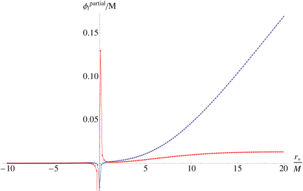
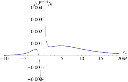
Figure 18: ‘Partial’ BC contribution to the $\ell$-mode for the radial component of the self-force for $s=0$ and $\ell=1$ as a function of $r_{*}$. (a) Continuous blue curve: BC contribution to the ‘$\ell$-mode of the partial field’ $\phi_{\ell}^{partial}/M$ of Eq.(34). Continuous red curve: its $r_{*}$-derivative. (b) $f_{\ell,r}^{partial}(r)/q$ of Eq.(35) in the static case (i.e., $\gamma=0$ and $d\tau/dt=(1-2M/r)^{1/2}$).

X Discussion

In this paper we have presented the first analytic method for calculating the branch cut modes in the non-asymptotic, ‘mid’-frequency regime in Schwarzschild space-time for fields of any integral spin. We have investigated their properties, in particular regarding their relation to quasinormal mode frequencies and around the algebraically special frequency. We have applied our calculation of the BC modes to investigate their partial (i.e., from $t>2|r_{*}|$) contribution for one $\ell$-mode to the self-force on a scalar charge moving on Schwarzschild background at constant radius. We have found that, for the particular case investigated, the BC contribution becomes larger as $t$ approaches $2|r_{*}|$ (where the high-frequency asymptotics of the BC modes become important) but the QNM contribution dominates the self-force at most times.

In Casals et al. (2009b) the first successful application of the so-called method of matched expansions for the calculation of the self-force was achieved. This method consists on calculating the Green function at ‘early times’ using a quasilocal expansion and in the ‘distant past’ using a Fourier mode and multipole decomposition of the Green function as in Eq.(1). In Casals et al. (2009b) the method was applied to the specific case of a black hole toy model space-time, namely the Nariai space-time, where the Green function possesses QNMs but not a BC and so the Green function in the ‘distant past’ is fully determined by the QNM series. In Schwarzschild space-time, on the other hand, the QNM series must be complemented by a BC integral. In Dolan and Ottewill (2011) the QNM series was calculated for large-$\ell$ and it was shown that it yields an interesting global singularity structure of the Green function. In this paper we have presented a method for calculating the BC integral and we have applied it to one $\ell$-mode. In Casals et al. we plan to apply a calculation of the BC integral for all $\ell$-modes, add it to a similar calculation of the QNM series and supplement it with a quasilocal expansion at ‘early times’ in order to calculate the full self-force in Schwarzschild space-time using the method of matched expansions.

Another situation where it is important to investigate the contribution of the BC is that of the response of a black hole to an initial perturbation. In this case, we expect that the BC contributes at ‘early’ times (that is, for $t$ close to $|r_{*}|+|r_{*}|$) as well as at late times (where a logarithmic behaviour precedes the known power-tail decay Casals and Ottewill (2012a)). We investigate the latter in depth in Casals and Ottewill .

On the quantum side, the asymptotically constant spacing in the imaginary part of the highly-damped QNM frequencies led to suggestions of a link with the quantization of the black hole area Hod (1998); Maggiore (2008). In Casals and Ottewill (2012b) we showed that, in the large-$\bar{\nu}$ regime, the spacing in the imaginary part of the QNM frequencies asymptotically equals that of the zeros of the BC modes for all spins $s=0,1$ and $2$. In this paper we have shown that, in the ‘mid’-frequency regime, these two spacings also remain very close in the cases $s=1$ and $2$ studied, while they differ more significantly in the case $s=0$. Intriguingly, the algebraically special frequency for gravitational perturbations plays a special rôle in the connection between QNMs and the BC, not only harbouring in its neighbourhood an almost purely imaginary QNM frequency but also marking the onset of the highly-damped regime for QNMs. In a different work, highly-damped QNMs in Kerr space-time have been interpreted as semiclassical bound states along a specific contour in the complex-$r$ plane and have been linked to Hawking radiation Keshet and Neitzke (2008). The least-damped QNMs have also been linked to Hawking radiation York Jr. (1983). Given that QNM frequencies, particularly in the spin-1 case, ‘approach’ the branch cut Casals and Ottewill (2012b) in the high-damping limit and that a connection with the branch cut also appears to exist in the ‘mid’-frequency regime, it would be interesting to investigate whether branch cut modes may play any rôle in the quantum properties of black holes.

An impending generalization of our current results in Schwarzschild is that to a rotating, Kerr black hole space-time. In principle, our method is readily generalizable to the rotating case, since Leaver’s series representations for the radial solutions are already valid in Kerr Leaver (1986b). Immediately, however, some significant differences appear with respect to the non-rotating Schwarzschild case. For example, the corresponding symmetry (8) in Kerr also involves a change in the sign of the azimuthal angular number, on which the radial solutions depend in the rotating case. As a consequence, the radial solution $f_{\ell}$ is not necessarily real along the branch cut and the discontinuity of $g_{\ell}$ across the branch cut is generally not only in its imaginary part but also in its real part, and so the BC ‘strength’ $q(\nu)$ is not necessarily real-valued. To further spice up the analysis in Kerr, the angular eigenvalue has various branch points in the complex-frequency plane (see, e.g., Barrowes et al. (2004)). This intricate and delicate structure of the modes in Kerr has various physical manifestations. We plan to investigate these issues in a future publication.

Appendix A Irregular confluent hypergeometric $U$-function

In this appendix we give some properties of the irregular confluent hypergeometric $U$-function, which we have used in the main body of the paper.

A useful integral representation of the $U$-function is given in, e.g., Eq.13.4.4 bk: :

$$U(a,b,z)=\frac{1}{\Gamma(a)}\int_{0}^{\infty}dt\ e^{-zt}t^{a-1}(1+t)^{b-a-1},\quad\text{Re}(a)>0,|\text{ph}(z)|<\pi/2$$ (36)

We require asymptotics for large values of the first argument of the $U$-function. For large, negative values of the first argument we use Eqs.13.8.10 and 10.17.3 bk: to obtain

$$U(a,b,x)\sim\Gamma\left(\frac{b}{2}-a+\frac{1}{2}\right)e^{x/2}x^{1/4-b/2}\left(\frac{\sqrt{2}}{\pi\sqrt{b-2a}}\right)^{1/2}\cos\left(\sqrt{2x(b-2a)}+\pi\left(a-\frac{b}{2}+\frac{1}{4}\right)\right),\quad a\to-\infty,b\geq 1,x>0$$ (37)

For large, positive values of the first argument we use Eqs.13.8.8 and 10.25.3 bk: to obtain

$$U(a,b,x)\sim\frac{e^{x/2}}{\Gamma(a)}\left(\sqrt{\frac{|x|}{a}}e^{i\psi/2}\right)^{1-b}\sqrt{\frac{\pi}{\sqrt{|x|a}e^{i\psi/2}}}e^{-2\sqrt{|x|a}e^{i\psi/2}},\quad a\to+\infty,\ b\leq 1,\ \psi\equiv\arg(x)\in(-\pi,+\pi]$$ (38)

.

Finally, from Eqs.13.2.4 and 13.2.41 bk: we obtain the following expression for the discontinuity across the branch cut of the $U$-function,

$$\left(ze^{-2\pi i}\right)^{a}U(a,b,ze^{-2\pi i})-z^{a}U(a,b,z)=\frac{2\pi ie^{z}(-z)^{a}}{\Gamma(a)\Gamma(1+a-b)}U(b-a,b,-ze^{-2\pi i})$$ (39)