“Pull moves” for rectangular lattice polymer models are not fully reversible

Abstract

“Pull moves” is a popular move set for lattice polymer model simulations. We show that the proof given for its reversibility earlier is flawed, and some moves are irreversible, which leads to biases in the parameters estimated from the simulations. We show how to make the move set fully reversible.

“Pull moves” for rectangular lattice polymer models are not fully reversible

Dániel Györffy, Péter Závodszky and András Szilágyi

©2012 IEEE. Personal use of this material is permitted. Permission from IEEE must be obtained for all other uses, in any current or future media, including reprinting/republishing this material for advertising or promotional purposes, creating new collective works, for resale or redistribution to servers or lists, orreuse of any copyrighted component of this work in other works.

This paper has been accepted for publication in IEEE/ACM Transactions on Computational Biology and Bioinformatics. The manuscript was first submitted on March 29, 2012, revised August 5, 2012, accepted September 29, 2012.

1 Introduction

Lattice polymer models have long been used for theoretical studies of various aspects of polymer behavior [1, 2]. In the HP lattice model of proteins [3], a chain is represented as a self-avoiding walk on a rectangular (square or cubic) lattice and the sequence space is reduced to two types of beads: a hydrophilic one (denoted as P) and a hydrophobic one (denoted as H). Analyses carried out on HP lattice protein models provided the foundations of the modern theory of protein folding [4].

For short polymers, exhaustive enumeration can be carried out, but for longer chains, excessive computational requirements permit only sampling the conformational space. Several efficient sampling methods have been developed such as the Metropolis–Hastings Monte Carlo method [5], equi-energy sampling [6] and Wang–Landau sampling [7, 8]. The main goal of the sampling may be finding the conformation with the lowest energy, generating a canonical ensemble of conformations, or estimating various parameters such as the density of states, free energies, thermodynamic averages, etc.

Figure 1: An example for an irreversible pull move. Conformation (a) is a chain with a straight end. A particular end move results in a hook at the end of the chain, conformation (b). But a reverse move is not possible because pulling the chain in the other direction results in a chain with a bent end (c) instead of a straight end. Excluding the move from (a) to (b) will not affect ergodicity because it remains possible to get from (a) to (b) by two moves, through (c). Note that the figure only shows an example; all end moves that result in a hooked end are irreversible.

All of these sampling methods require a mutation step. For rectangular lattice models, several move sets have been developed to serve as a mutation operator. In pivot moves [9, 10], one of the beads serves as a pivot point and a symmetry operation is carried out. Pivot moves are ergodic but due to the significant change in conformation, the acceptance rate is very low for compact conformations [10, 11]. In the class of k-bead moves, a predefined number (k) of contiguous beads are relocated [2], but these moves are not ergodic for longer chains [12]. A fundamentally different method is bond-rebridging [13], which provides a high acceptance rate at the cost of not being ergodic [14, 11].

Lesh and coworkers introduced a new local move set, called pull moves [15], and provided proof that the move set is ergodic and reversible. There are two types of pull moves. In one type, a four-bead loop is formed and the chain is pulled until the end is reached or an existing loop is straightened. To ensure reversibility, another move type was introduced where one end of the chain is pulled until a loop is eliminated [15, 6]. “Pull moves” has become a popular and commonly used move set for lattice polymer simulations. It has been used in replica exchange Monte Carlo simulations [16] and applications of equi-energy [6] and Wang–Landau sampling [8, 14, 17, 11] and tabu search [15, 18]. It has been adapted for triangular and hexagonal lattice polymers [19, 20].

2 Results

Applications of pull moves have been implemented assuming that the move set is reversible (i.e. that the reverse of each valid move from state A to state B is also a valid move from B to A), based on the proof of reversibility given by Lesh et al. [15]. However, examining the proof, we noticed that it contains a flaw as it overlooks the fact that one type of end move is actually not reversible. (The irreversibility does not affect pull moves on triangular and hexagonal lattices.)

Here, we provide a proof that one type of end pull moves is irreversible. Let us number the beads of the chain from $1$ to $n$. The irreversibility affects those end moves that result in a hook at the end of the chain as shown in Figure 1(b). By this move, both beads $1$ and $2$ move to a new location such that bead $1$ will be adjacent to the old location of bead $2$. According to the rules of pull moves described in Lesh et al. [15], this move can be reversed by pulling the chain in the other direction until a valid conformation is reached. However, when we try to perform this reverse move, bead $2$ will return to its original position, but because this position is adjacent to the new location of bead $1$, the chain will be in a valid conformation without moving bead $1$. Thus, bead $1$ is not returned to its original position. The same reasoning applies to beads $n$ and $n-1$. Figure 1 shows one example of the irreversibility where, starting from a chain with a straight end, one move results in a hook at the end of the chain, but the supposed reverse move produces a chain with a bent end.

For a 2D chain with length $L$, the maximum number of possible internal and end pull moves is $4(L-2)$ and $18$, respectively; for 3D chains, the corresponding numbers are $8(L-2)$ and $25$. Four of the $18$ end pull moves in 2D, and $8$ of the $25$ end pull moves in 3D are irreversible. We calculated that $15\ \%$ of edges in the transition graph of a 2D 10-bead chain represent an irreversible transition.

Monte Carlo sampling schemes, including Wang–Landau sampling, rely on the principle of detailed balance which requires microscopic reversibility. When microscopic reversibility is violated, cycles of microstates will arise, and statistical weights derived from the simulations will be incorrect.

Fortunately, the irreversibility can easily be fixed by simply excluding the irreversible moves, i.e. those moves that produce a hook at the end of the chain like that depicted in Figure 1. This new, reduced move set preserves ergodicity; this is easily seen in Figure 1 as direct moves from (a) to (c) and (c) to (a) are both allowed.

If the sampling algorithms are implemented without simplifications, the irreversible moves will never be accepted, leading only to a waste of CPU time. However, implementations often use the assumption of reversibility to introduce simplifications, leading to irreversible moves being accepted, and thus, a bias in the sampling.

In Monte Carlo samplings, such as e.g. Wang–Landau sampling, the transition probability is proportional to the rates of the a priori probabilities of the transition from one state to the other and vice versa:

$$p\left(A\rightarrow B\right)\propto\frac{p_{ap}\left(B\rightarrow A\right)}{p_{ap}\left(A\rightarrow B\right)}.$$ (1)

The a priori probability of a transition is

$$p_{ap}\left(A\rightarrow B\right)=\frac{n\left(A\rightarrow B\right)}{n\left(A\right)}$$ (2)

where $n\left(A\rightarrow B\right)$ is the number of transitions from the state $A$ to state $B$ and $n\left(A\right)$ is the number of transitions originating from $A$. If a move is irreversible such that $n(B\rightarrow A)=0$ (as is the case for the irreversible end moves), then $p(A\rightarrow B)$ will be zero and this move will never be accepted during the simulation. Thus, CPU time will be wasted but the sampling will be correct.

However, when implementing the sampling algorithm, a simplified expression for $p(A\rightarrow B)$ may be used instead of Equation (1). If the move set is assumed reversible then

$$n\left(A\rightarrow B\right)=n\left(B\rightarrow A\right),$$ (3)

and we can simplify Equation (1) so that

$$p\left(A\rightarrow B\right)\propto\frac{n\left(A\right)}{n\left(B\right)}.$$ (4)

With an irreversible move set, Equation (3) is not valid and Equation (4) yields nonzero probabilities even for irreversible moves. This leads to accepting irreversible moves and, consequently, incorrect sampling.

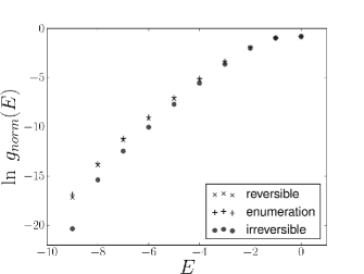
Figure 2: Logarithm of the normalized density of states ($g_{norm}\left(E\right)$) for the 2D 20mer HPHPPHHPHPPHPHHPPHPH, also investigated in [21], from Wang–Landau simulations (50 runs averaged) with reversible and irreversible pull moves, and from exhaustive enumeration. Wang–Landau sampling was stopped when the logarithm of the modification factor fell below $10^{-8}$. The flatness criterion was chosen to be $p=0.8$

To investigate the effect of neglecting the irreversibility, we estimated the density of states of a 2D 20mer by Wang–Landau simulations [7] using both the original (irreversible) and the fixed (reversible) move set (applying the simplification in Equation (4)), and compared them with the exact values obtained by exhaustive enumeration (Figure 2). As the figure shows, by using the irreversible moves, the density of states is significantly underestimated for most energy levels, especially for the lowest ones. We obtained similar but less marked differences for a 2D 64mer, a 3D 103mer, and a 18mer homopolymer also investigated previously [21, 17, 22].

3 Discussion

We have shown that some end pull moves are irreversible, and ignoring the irreversibility may lead to inaccurate sampling. Whether and to what extent this irreversibility affected the results of earlier studies is an open question. Although we cannot rule out the possibility that some authors recognized the irreversibility and excluded the irreversible moves, all papers we examined state that pull moves are reversible and we found no mention of excluding any moves. Even if irreversible moves were not explicitly excluded in a study, this may not have had a noticeable effect on the results for several reasons: (i) the study only used pull moves for finding the ground state, so the irreversibility did not affect it [15, 16, 18]; (ii) the authors may have used the full formula (Equation (1)) to calculate transition probabilities, thus the irreversible moves were tried but always rejected; (iii) the study was done on long chains where end moves represent only a small fraction of all moves, thus their irreversibility only had a small effect.

In many cases, studies do not provide enough details on the implementation of the used algorithm and their results to allow us an assessment of whether and how irreversibility may have affected the results. A few studies [6, 8, 22] provide an accuracy analysis, comparing the density of states obtained from the simulations with that from exact enumeration [6, 8], and they only find small differences from the exact values. However, they do not state whether they used the full formula (Equation (1)) or its simplified form (Equation (4)); only the simplified form leads to inaccuracies. On the other hand, studies that explicitly state that they used the simplified formula (Equation (4)) [17, 14] do not provide an accuracy analysis (e.g. because of working with long chains where enumeration is not possible), so it is impossible to judge the accuracy of their results. An exception is the study of Swetnam and Allen [22], which both calculates accuracy and states that the simplified formula (Equation (4)) was used. However, their calculations are for a 18mer homopolymer where, according to our own calculations, the difference caused by the irreversibility is small. Besides, they use various algorithms with varying results, and we are unable to directly compare their results with ours. Thus, we cannot determine with certainty whether potential irreversibility affected their results.

There is a publicly available software package, LatPack [23], that implements pull moves. We tested the program and found that it fails to exclude the irreversible end pull moves.

4 Conclusion

As our demonstrations indicate, accurate calculations in the future should be based on simulations using the fixed version of pull moves as described in the present article. The simple recipe is that all end pull moves that result in a hook at the end of the chain should be excluded.

References

- [1] P. H. Verdier and W. H. Stockmayer, “Monte Carlo calculations on the dynamics of polymers in dilute solution,” J Chem Phys, vol. 36, pp. 227–235, 1962.
- [2] O. J. Heilmann and J. Rotne, “Exact and Monte Carlo computations on a lattice model for change of conformation of a polymer,” J Stat Phys, vol. 27, pp. 19–35, 1982.
- [3] K. F. Lau and K. A. Dill, “A lattice statistical mechanics model of the conformational and sequence spaces of proteins,” Macromolecules, vol. 22, pp. 3986–3997, 1989.
- [4] K. A. Dill, S. Bromberg, K. Yue, K. M. Fiebig, D. P. Yee, P. D. Thomas, and H. S. Chan, “Principles of protein folding–a perspective from simple exact models.” Protein Sci, vol. 4, pp. 561–602, 1995.
- [5] W. K. Hastings, “Monte Carlo sampling methods using Markov chains and their applications,” Biometrika, vol. 57(1), pp. 97–109, 1970.
- [6] S. C. Kou, J. Oh, and W. H. Wong, “A study of density of states and ground states in hydrophobic-hydrophilic protein folding models by equi-energy sampling.” J Chem Phys, vol. 124, p. 244903, 2006.
- [7] F. Wang and D. P. Landau, “Efficient, multiple-range random walk algorithm to calculate the density of states.” Phys Rev Lett, vol. 86, pp. 2050–3, 2001.
- [8] T. Wüst and D. P. Landau, “The HP model of protein folding: a challenging testing ground for Wang-Landau sampling,” Computer Physics Communications, vol. 180, pp. 475–9, 2008.
- [9] M. Lal, “’Monte Carlo’ computer simulation of chain molecules I.” Molecular Physics, vol. 17(1), pp. 57–64, 1969.
- [10] N. Madras and A. D. Sokal, “The pivot algorithm: a highly efficient Monte Carlo method for the self-avoiding walk,” J Stat Phys, vol. 50, pp. 109–186, 1988.
- [11] T. Wüst, Y. W. Li, and D. P. Landau, “Unraveling the beautiful complexity of simple lattice model polymers and proteins using Wang–Landau sampling,” J Stat Phys, vol. 144, pp. 638–51, 2011.
- [12] N. Madras and A. D. Sokal, “Nonergodicity of local, length-conserving Monte Carlo algorithms for the self-avoiding walk,” J Stat Phys, vol. 47, pp. 573–595, 1987.
- [13] J. M. Deutsch, “Long range moves for high density polymer simulations,” J Chem Phys, vol. 106, pp. 8849–8854, 1997.
- [14] T. Wüst and D. P. Landau, “Versatile approach to access the low temperature thermodynamics of lattice polymers and proteins,” Phys Rev Lett, vol. 102(17), p. 178101, 2009.
- [15] N. Lesh, M. Mitzenmacher, and S. Whitesides, “A complete and effective move set for simplified protein folding,” in Proceedings of the seventh annual international conference on Research in computational molecular biology, ser. RECOMB ’03. New York, NY, USA: ACM, 2003, pp. 188–195. [Online]. Available: http://doi.acm.org/10.1145/640075.640099
- [16] C. Thachuk, A. Shmygelska, and H. H. Hoos, “A replica exchange Monte Carlo algorithm for protein folding in the HP model.” BMC Bioinformatics, vol. 8, p. 342, 2007.
- [17] A. D. Swetnam and M. P. Allen, “Improved simulations of lattice peptide adsorption.” Phys Chem Chem Phys, vol. 11, pp. 2046–55, 2009.
- [18] J. Błazewicz, P. Lukasiak, and M. Miłostan, “Application of tabu search strategy for finding low energy structure of protein.” Artif Intell Med, vol. 35, pp. 135–45, 2005.
- [19] H.-J. Böckenhauer, A. Dayem Ullah, L. Kapsokalivas, and K. Steinhöfel, “A local move set for protein folding in triangular lattice models,” in Algorithms in Bioinformatics, ser. Lecture Notes in Computer Science, K. Crandall and J. Lagergren, Eds. Springer Berlin / Heidelberg, 2008, vol. 5251, pp. 369–381.
- [20] M. Jiang and B. Zhu, “Protein folding on the hexagonal lattice in the HP model.” J Bioinform Comput Biol, vol. 3, pp. 19–34, 2005.
- [21] R. Unger and J. Moult, “Genetic algorithms for protein folding simulations.” J Mol Biol, vol. 231, pp. 75–81, 1993.
- [22] A. D. Swetnam and M. P. Allen, “Improving the Wang–Landau algorithm for polymers and proteins.” J Comput Chem, vol. 32, pp. 816–21, 2011.
- [23] M. Mann, D. Maticzka, R. Saunders, and R. Backofen, “Classifying proteinlike sequences in arbitrary lattice protein models using LatPack.” HFSP J, vol. 2, pp. 396–404, 2008.