Irregularities and Scaling in Signal and Image Processing: Multifractal Analysis

Abstract:

B. Mandelbrot gave a new birth to the notions of scale invariance, selfsimilarity and non-integer dimensions, gathering them as the founding corner-stones used to build up fractal geometry. The first purpose of the present contribution is to review and relate together these key notions, explore their interplay and show that they are different facets of a same intuition. Second, it will explain how these notions lead to the derivation of the mathematical tools underlying multifractal analysis. Third, it will reformulate these theoretical tools into a wavelet framework, hence enabling their better theoretical understanding as well as their efficient practical implementation. B. Mandelbrot used his concept of fractal geometry to analyze real-world applications of very different natures. As a tribute to his work, applications of various origins, and where multifractal analysis proved fruitful, are revisited to illustrate the theoretical developments proposed here.

Keywords: Scaling, Scale Invariance, Fractal, Multifractal, Fractional dimensions, Hölder regularity, Oscillations, Wavelet, Wavelet Leader, Multifractal Spectrum, Hydrodynamic Turbulence, Heart Rate Variability, Internet Traffic, Finance Time Series, Paintings

1 Introduction

As many students, before and after us, we first met Benoît Mandelbrot through his books [127, 128]; indeed, they were scientific bestsellers, and could be found in evidence in most scientific bookshops. A quick look was sufficient to realize that Benoît was an unorthodox scientist; these books radically differed from what we were used to, and were trespassing several taboos of the time: First, they could not be straightforwardly associated with any of the standardly labelled fields of science, which had been taught to us as separate subjects. This could already be inferred from their titles: The fractal geometry of nature [128] constitutes a statement that mathematics and natural sciences are intrinsically mixed, and that the purpose will not be to disentangle them artificially, but rather to explore their interactions. The contents of these books confirmed this first feeling: Though they contained a large proportion of very serious mathematics, they did not follow the old definition-theorem-proof articulation we were used to. The focus was directly on the observation of figures and on their pertinence for modeling; the mathematics were there to help and comfort the deep geometric intuition that Benoît had developed. This does not mean that he considered mathematics as an ancillary discipline. To the contrary, many testimonies confirm how enthusiastic he was when one of his mathematical intuitions was proven correct, and how he immediately incorporated the new mathematical methods in his own toolbox, which then helped him to sharpen his intuition and go further.

Another revolutionary point was that these books reversed the classical focusses: While one did find familiar mathematical objects (the nowhere differentiable Weierstrass functions, or the devil’s staircase had been encountered before), the role he made them play was radically different: So far, they had only been counterexamples, or pathological objects pedagogically used to shed light on possible pitfalls; instead of this restrictive role, Benoît used them as the key examples and cornerstones to found a new geometry based on roughness and selfsimilarity. These books were opening a subject, and drawing tracks through a new territory; their purpose was not to give the usual polished, final description of a well understood area, but to open windows on how science advances, and they had a strong influence on our vocations to research.

Later, personal meetings played a decisive role; let us only mention one such occasion: At the end of his PhD, one of us (S. J.) met Benoît who was visiting Ecole Polytechnique. Benoît had heard of wavelets, which, at the time, were a new tool still in infancy, and immediately envisaged possible interactions between wavelets and fractal analysis. A key feature of fractals is scaling invariance, and, because wavelets can be deduced one from the others by translations and dilations of a given function, their particular algorithmic structure should reveal the scaling invariance properties of the analyzed objects. Driven by his insatiable curiosity, Benoît wanted to learn everything about wavelets (which was actually not so much at the time!) and then, with his characteristic generosity, he shared with this student he barely knew his intuitions on the subject. Thus, the present contribution can be read as a tribute to some of the scientific lines Benoît had dreamed about at the time: It will show how and why wavelet techniques yield powerful tools for analyzing fractal properties of signals and images, and thus supply new collections of tools for their classification and modeling.

1.1 Scale invariance and self similarity

Exact (or deterministic) self similarity.  Fractal analysis can roughly be thought of as a way to characterize and investigate the properties of irregular sets. Note that irregularity is a negatively defined word; the description of the scientific domain it covers is therefore not clearly feasible, and had not been tried before B. Mandelbrot developed the concepts of fractal geometry. One of his leading ideas was a notion of regularity in irregularity or selfsimilarity: The object is irregular, but there is some invariance in its behavior across scales. For some sets, the notion of selfsimilarity replaces the notion of smoothness. For instance, the triadic Cantor set is selfsimilar, in the sense that it is made of two pieces which are the same as the whole set is shrunk by a factor 3. The purpose of multifractal analysis is to transpose this idea from the context of geometrical sets to that of functions. Sometimes, this transposition can be directly achieved, when the geometrical set consisting of the graph of the function also displays some selfsimilarity. Consider the example of the Weierstrass-Mandelbrot functions (a slight variant of the famous Weierstrass functions, see [128] pp. 388-390):

$${\cal W}_{a,H}(x)=\sum_{n=-\infty}^{+\infty}\frac{\sin(a^{n}x)}{a^{Hn}}\hskip 42.67912pt\mbox{for}\hskip 17.07164pta>1\hskip 17.07164pt\mbox{and }\hskip 17.07164ptH\in(0,1)$$ (1)

(note that the series converges when $n\rightarrow+\infty$ because $a>1$ and when $n\rightarrow-\infty$ because $|\sin(a^{n}x)|\leq|a^{n}x|$ and $H<1$). Those functions clearly satisfy the exact selfsimilarity relationship

$$\forall x\in{\mathbb{R}},\hskip 17.07164pt{\cal W}_{a,H}(ax)=a^{H}{\cal W}_{a,H}(x).$$ (2)

Note that selfsimilar functions associated with a selfsimilarity exponent $H>1$ can be obtained using slight variants: For instance, the function

$$\sum_{n=-\infty}^{+\infty}\frac{\cos(a^{n}x)-1}{a^{Hn}}\hskip 42.67912pt\mbox{for}\hskip 17.07164pta>1\hskip 17.07164pt\mbox{and }\hskip 17.07164ptH\in(0,2)$$

is selfsimilar with a selfsimilarity exponent $H$, which can go up to 2; and the function

$$\sum_{n=-\infty}^{+\infty}\frac{\sin(a^{n}x)-a^{n}x}{a^{Hn}}\hskip 42.67912pt\mbox{for}\hskip 17.07164pta>1\hskip 17.07164pt\mbox{and }\hskip 17.07164ptH\in(1,3)$$

is selfsimilar with a selfsimilarity exponent $H$ which can go up to 3. Note that this “renormalization technique” can be pushed further to deal with higher and higher values of $H$, yielding smoother and smoother functions: One thus obtains functions that are everywhere $C^{[H]}$ and nowhere $C^{[H]+1}$.

Random (or statistical) self similarity.  Functions satisfying (2) are very rare; therefore the notion of exact selfsimilarity can be considered too restrictive for real world data modeling. Fruitful generalizations of this concept can be developed into several directions. A first possibility lies in weakening the exact deterministic relationship (2) into a probabilistic one: The (random) functions $a^{H}f(ax)$ do not coincide sample path by sample path, but share the same statistical laws. A stochastic process $X_{t}$ is said to be selfsimilar, with selfsimilarity exponent $H$ iff

$$\forall a>0,\;\;\;\{X_{at},\;t\in{\mathbb{R}}\}\;\stackrel{{\scriptstyle{\cal L}}}{{=}}\{a^{H}X_{t},\;t\in{\mathbb{R}}\}$$ (3)

(see Definition 5 where the precise definition of equality in law of processes is recalled).

The first example of such selfsimilar processes is that of fractional Brownian motion (hereafter referred to as fBm), introduced by Kolmogorov [105]. Its importance for the modeling of scale invariance and fractal properties in data was made explicit and clear by Mandelbrot and Van Ness in [138]. This article is characteristic of Mandelbrot’s genius, which could perceive similarities between very distant disciplines: Motivations simultaneously rose from hydrology (cumulated water flow), economic time series and fluctuations in solids. Notably, B. Mandelbrot explained that fBm (with $0.5<H<1$) was well-suited to model long term dependencies, or long memory effects, in data, a property he liked to refer to as the Joseph effect in a colorful and self-speaking metaphoric comparison to the character of the Bible (cf. e.g., [139]). Selfsimilar processes have since been the subject of numerous exhaustive studies, see for instance the books [4, 55, 65, 168]. Note also that B. Mandelbrot put selfsimilarity (which he actually more accurately called selfaffinity) as a central notion in the study stochastic processes in views of applications, see [136] for a panorama of his works in this direction.

1.2 Selfsimilarity and Wavelets

Let us now briefly come back to B. Mandelbrot’s intuition and see how wavelet analysis can reveal relationships such as (2) or (3), as well as other important probabilistic properties of stochastic processes. In its simplest form, an orthonormal wavelet basis of $L^{2}({\mathbb{R}})$ is defined as the collection of functions

$$2^{j/2}\psi(2^{j}x-k),\;\;\mbox{ where}\;\;j,k\in{\mathbb{Z}},$$ (4)

and the wavelet $\psi$ is a smooth, well localized function. Wavelet coefficients are further defined by

$${c_{j,k}=2^{j}\int f(x)\;\psi(2^{j}x-k)\;dx.}$$

A $L^{1}$-normalization is used (rather than the classical $L^{2}$-normalization), as it is better suited to express scale invariance relationships, as shown in (5) below.

Let $f$ denote a function satisfying (2) with $a=2$, i.e. such that

$$\forall x\in{\mathbb{R}},\hskip 17.07164ptf(2x)=2^{H}f(x);$$

then, clearly, its wavelet coefficients satisfy

$$\forall j,k,\hskip 22.76219ptc_{j,k}=2^{H}c_{j+1,k}.$$

Similarly, in the probabilistic setting, if (3) holds, then the (infinite) sequences of random vectors ${\cal C}_{j}\equiv(2^{Hj}c_{j,k})_{k\in{\mathbb{Z}}}$ satisfy the following property:

$$\{{\cal C}_{j}\}_{j\in{\mathbb{Z}}}\hskip 11.38109pt\mbox{ share the same law.}$$ (5)

Other probabilistic properties have simple wavelet counterparts; let us mention a few of them.

Let $X_{t}$ be a Markov process, i.e. a stochastic process satisfying the property

$$\mbox{ $\forall s>0$, $X_{t+s}-X_{t}$ is independent of the $(X_{u})_{u\leq t}$ };$$

typical examples of Markov processes are supplied by Brownian motion, or, more generally, by Lévy processes, i.e. processes with stationary and independent increments. Because wavelets have vanishing integrals, the Markov property implies that, if the supports of the $\psi(2^{j}x-k)$ are disjoint, then the corresponding coefficients $c_{j,k}$ are independent random variables.

Recall that a stochastic process $X_{t}$ has stationary increments iff

$$\mbox{ $\forall s>0$, $X_{t+s}-X_{t}$ has the same law as $X_{s}$ };$$

typical examples are fractional Brownian motions, or Lévy processes. If $X_{t}$ has stationary increments, then

$$\forall j,\;\;\mbox{ the random variables }\;(c_{j,k})_{k\in{\mathbb{Z}}}\;\mbox{ share the same law. }$$ (6)

Note that this property holds for each given $j$, but implies no relationship between wavelet coefficients at different scales; however, if $X_{t}$ is a selfsimilar process of exponent $H$ with stationary increments, then it follows from (5) and (6) that the random variables $2^{Hj}c_{j,k}$ all share the same law (for all $j$ and $k$).

A random variable $X$ has a stable distribution iff

$$\forall a,b\geq 0,\;\;\exists c>0\;\mbox{ and}\;d\in{\mathbb{R}}\;\;\;\mbox{ such that }\;\;\;\;\;aX_{1}+bX_{2}\stackrel{{\scriptstyle{\cal L}}}{{=}}cX+d$$

where $X_{1}$ and $X_{2}$ are independent copies of $X$. A random process is stable if all linear combinations of the $X(t_{i})$ are stable. This property implies that the wavelet coefficients of a stable process are stable random variables. Further, it can actually be shown that any finite collection of wavelet coefficients forms a stable vector (cf. e.g., [7, 162, 163, 175]).

Finally, if $X_{t}$ is a Gaussian process, then any finite collection of its wavelet coefficients is a Gaussian vector. Note however a common pitfall: Unless some additional stationarity property holds, the sole Gaussianity hypothesis for the marginal distribution of the process does not imply that the empirical distributions of the coefficients $(c_{j,k})_{k\in{\mathbb{Z}}}$ are close to Gaussian: It can only be said that they will consist of Gaussian mixtures (which can strongly depart from a Gaussian distribution). The statistical properties of wavelet coefficients of fBm were studied in depth in the seminal works of P. Flandrin [71, 72] that significantly contributed to the popularity of wavelet transforms in the analysis of scale invariance.

Among the results that we mentioned above, it is important to draw a difference between those that are a consequence of the sole fact that wavelet coefficients are defined as a linear mapping, and therefore would hold for any other basis (Gaussianity and stability) and those that are the consequence of the particular algorithmic nature of wavelets (selfsimilarity and stationarity). These (rather straightforward) results are either implicit or explicit in the literature concerning wavelet analysis of stochastic processes; however, in order to give a flavor of the ideas and methods involved, we give a proof of (5) at the end of Section 4.1.

Further, let us mention that all these wavelet properties do not constitute exact characterizations of the probabilistic properties of the corresponding processes, but only implications, because of a deficiency of wavelet expansions that will be explained in Section 4.1.

1.3 Beyond selfsimilarity: Multifractal analysis

Beyond selfsimilarity.  An obvious drawback of using exact probabilistic properties, such as selfsimilarity, or independence of increments is that, though they can relevantly model physical properties of the underlying data, they usually do not hold exactly for real-life signals. Two limitations of selfsimilarity can classically be pointed out. First, the scaling properties may not hold for all scales (as required by the mathematical definition of selfsimilarity). This may be due to noise corruption or it may also result from the fact that the physical phenomena implying those properties intrinsically act over a finite range of scales only. Second, the appealing property of selfsimilarity (the sole selfsimilarity parameter $H$ contains the essence of the model) may also constitute its limitation: Can one really expect that the complexity of real-world data can be accurately encapsulated in one single parameter only? Let us examine such issues.

Multiplicative Cascades.  As mentioned above, B. Mandelbrot coined fBm as one of the major candidates to model scale invariance. However, combining selfsimilarity and stationary increments implies that all finite moments of the increments of fBm (and of any process whose definition gathers these two properties) verify, for all $p$s such that ${\hbox{I\kern-1.99997pt\hbox{E}}}(|X(1)|^{p})<\infty$ [168, 65],

$$\forall\tau\in{\mathbb{R}},\hskip 17.07164pt{\hbox{I\kern-1.99997pt\hbox{E}}}(|X(t+\tau)-X(t)|^{p})={\hbox{I\kern-1.99997pt\hbox{E}}}(|X(1)|^{p})\;|\tau|^{pH}.$$ (7)

Though very powerful, this result can also be regarded as a severe limitation for applications, where empirical estimates of moments, $\int|X(t+\tau)-X(t)|^{p}dt$, computed on the data assuming ergodicity, may instead behave as: $\int|X(t+\tau)-X(t)|^{p}dt=\tau^{\zeta(p)}$, for a range of $\tau$, and where $\zeta(p)$ is, by construction, a concave function, but is not necessarily linear. This is notably the case when analyzing velocity or dissipation fields in the study of hydrodynamic turbulence where strictly concave scaling functions were obtained (cf. e.g., [76] for a review of experimental results). This was justified by a celebrated argument due to Kolmogorov and Obukhov in 1962 [108, 149, 186]: Navier-Stokes equation, governing fluid motions, implies that the (third power of the) gradient of the velocity $u(x+r)-u(x)$ is proportional to the mean of the local energy $\epsilon_{r}$ dissipated into a bulk of size $r$: ${\hbox{I\kern-1.99997pt\hbox{E}}}(u(x+r)-u(x))^{3}\propto{\hbox{I\kern-1.99997pt\hbox{E}}}(\epsilon_{r})\cdot r$. If $\epsilon_{r}$ is constant, then any power scales as ${\hbox{I\kern-1.99997pt\hbox{E}}}(u(x+r)-u(x))^{p}\propto\epsilon_{r}^{p}r^{p/3}$. But, in turbulence, $\epsilon_{r}$ is not constant over space and should rather be regarded as a random variable, hence implying: ${\hbox{I\kern-1.99997pt\hbox{E}}}(u(x+r)-u(x))^{p}\propto{\hbox{I\kern-1.99997pt\hbox{E}}}(\epsilon_{r}^{p})\;r^{p/3}$ which naturally implies a general scaling of the form $\sim{\hbox{I\kern-1.99997pt\hbox{E}}}(u(x+r)-u(x))^{p}\propto r^{\zeta(p)}$, with $\zeta(p)$ which is likely to depart from the linear behavior $pH$ which is implied by the selfsimilarity hypothesis.

To account for this form of observed scale invariance, new stochastic models have been proposed: Multiplicative cascades. Numerous declinations of cascades were proposed in the literature of hydrodynamic turbulence to model data, see e.g., [76] (on the mathematical side, see the book [26] for a detailed review, and also the contribution of J. Barral and J. Peyrière [32] in the present volume, for a lighter introduction). For the sake of simplicity, the simplest (1D) formulation is presented here; however, it contains the key ingredients present in all other more general cascade models. Starting from an interval (arbitrarily chosen as the unit interval), a cascade is constructed as the repetition of the following procedure ($c$ being an arbitrary integer): At iteration $j$, each of the $c^{j-1}$ sub-intervals $\{I_{j-1,k},k=0,\ldots c^{j-1}-1\}$, obtained at iteration $j-1$, is split into $c$ intervals of the same length $c^{-j}$; a mean-$1$ positive random variable $w_{j,k}$ (drawn independently and with identical distribution) is associated with each $\{I_{j,k},k=0,\ldots c^{j}-1\}$. After an infinite number of iterations, the cascade $W$ is defined as the limit (in the sense of measures) of the finite products

$$W_{J}(x)dx=\displaystyle\prod_{j\leq J,\;x\in I_{j,k}}w_{j,k}\;dx.$$

Mathematically, this sequence of measures converges under mild conditions on the distribution of the multipliers $w$ (cf. [103]). Such constructions and variations have been massively used to model the Richardson energy cascade implied by the Navier-Stokes equation [164] (cf. [76] for a review of such models). One of the major contributions of B. Mandelbrot to the field of hydrodynamic turbulence was proposed in [124], where he presented the themes and variations on multiplicative cascades in a single framework and studied their common properties, notably in terms of scale invariance. This celebrated contribution paved the way towards the creation of the word multifractal, to the notions of multifractal processes and multifractal analysis, where multi here refers to the fact that instead of a single scaling exponent $H$, a whole family of exponents $\zeta(p)$ are needed for a better description of the data. B. Mandelbrot also discussed the importance of the distribution of the multipliers and how multiplicative cascades may significantly depart from log-normal statistics that could be obtained from a simplistic argument:

$$\Pi w_{j,k}=\Pi e^{\log(w_{j,k})}=e^{\sum\log w_{j,k}},$$

where $\sum\log w_{j,k}$ tends to a normal distribution, hence $e^{\sum\log w_{j,k}}$ should tend to a log-normal distribution (cf. [132, 123], and also [186]). This opened many research tracks proposing alternatives to the log-normal model, the most celebrated one being the log-Poisson model [172]. This will be further discussed in Section 6.1. Much later, multiplicative cascades were connected to Compound Poisson cascades and further to Infinitely Divisible Distributions (cf. e.g., [148]). Mandelbrot himself contributed to these latter developments with the earliest vision of Compound Poisson Cascades [30] and also with his celebrated fBm in multifractal time [135], which will be considered in Section 6.2. This gave birth to multiple constructions of processes with multifractal properties (cf. e.g., [19, 23, 24, 33, 34, 48, 49]).

Compared with the concept of selfsimilarity (and in particular fBm), which is naturally related to random walks and hence to additive constructions, cascades are, by construction, tied to a multiplicative structure. This deep difference in nature explains why practitioners, for real-world applications, are often eager to distinguish between these two classes of models. This distinction is however often misleadingly confused with the opposition of mono- versus multi-fractal processes. This will be further discussed in Section 5.4.

Scaling functions and scaling exponents.  The empirical observations of strictly concave scaling exponents, made on hydrodynamic turbulence data, led to the design of a new tool for analysis: Scaling functions. Let $f:{\mathbb{R}}^{d}\rightarrow{\mathbb{R}}$. The Kolmogorov scaling function of $f$ (see [107]) is the function $\eta_{f}(p)$ implicitly defined by the relationship

$$\forall p\geq 1,\hskip 22.76219pt\int|f(x+h)-f(x)|^{p}dx\quad\sim\quad|h|^{\eta_{f}(p)},$$ (8)

the symbol $\sim$ meaning that

$$\eta_{f}(p)=\lim_{|h|\rightarrow 0}\frac{\log\left(\displaystyle\int|f(x+h)-f(x)|^{p}dx\right)}{\log|h|}.$$ (9)

Note that this limit does not necessarily always exist; when it does, it reflects the fact that $f$ shows clear scaling properties (and it is needed to hold in order to numerically compute scaling functions). However, we are not aware of any simple and general mathematical assumption implying that it does; therefore, it is important to formulate a mathematical and slightly more general definition of the scaling function, which is well defined for any function $f\in L^{p}$:

$$\forall p\geq 1,\hskip 17.07164pt\eta_{f}(p)=\liminf_{|h|\rightarrow 0}\frac{\log\left(\displaystyle\int|f(x+h)-f(x)|^{p}dx\right)}{\log|h|}.$$ (10)

It is important to note that, if data are smooth (i.e., if one obtains that $\eta_{f}(p)\geq p$), then one has to use differences of order 2 or more in (9) and (10) in order to define correctly the scaling function.

For application to real-world data, which are only available with a finite time or space resolution, (9) can be interpreted as a linear regression of the log of the left hand side of (8) vs. $\log(|h|)$. The same remark holds for the other scaling functions that we will meet.

Multifractal analysis.  In essence, multifractal analysis consists in the determination of scaling functions (variants to the original proposition of Kolmogorov $\eta_{f}$ will be considered later). Such scaling functions can then be involved into classification or model selection procedures. Scaling functions constitute a much more flexible analysis tool than the strict relation (2). For many different real-world data stemming from applications of various natures, relationships such as (8) are found to hold, while this is usually not the case for (2), see Section 6 for illustrations on real world data.

An obvious key advantage of the use of the scaling function $\eta_{f}(p)$ is that its dependence in $p$ can take a large variety of forms, hence providing versatility in adjustment to data. Therefore, multifractal analysis, being based on a whole function (the scaling function $\eta_{f}(p)$, or some of its variants introduced below), rather than on the single selfsimilarity exponent, yields much richer tools for classification or model selection. The scaling function however satisfies a few constraints, for example, it has to be a concave non-decreasing function (cf. e.g., [99, 183]).

Another fundamental difference between the selfsimilarity exponent and the scaling function lies in the fact that, for stochastic processes, the selfsimilarity exponent is, by definition, a deterministic quantity, whereas the scaling function is constructed for each sample path, and therefore is a priori defined as a random quantity. And, indeed, even if the limit in (10) turns out to be deterministic for many examples of stochastic processes (such as fBm, Lévy processes, or multiplicative cascades, for instance), it is not always the case, as shown, for instance, by the example of fairly general classes of Markov processes, such as the ones studied in [27]. Note that, if a stationarity assumption can be reasonably assumed, then one can define a deterministic quantity by taking an expectation instead of a space average in (10), which leads to a definition of the scaling function through moments of increments. Under appropriate ergodicity assumptions, time (or space) averages can be shown to coincide with ensemble averages, and, in this case, both approaches lead to the same scaling functions, see [165] for a discussion (checking such ergodicity assumptions for experimental data does, however, not seem feasible and can become an intricate issue, cf. [112]).

1.4 Data analysis and Signal Processing

In its early ages, the concept of scale invariance has been deeply tied to that of $1/f$-processes, that is, to second order stationary random processes whose power spectral density behave as a power law with respect to frequency over a broad range of frequencies: $\Gamma_{X}(f)\sim C|f|^{-\beta}$, where the frequency $f$ satisfies $f_{m}\leq f\leq f_{M}$, with $f_{M}/f_{m}\gg 1$. From that starting point, spectrum analysis was regarded as the natural tool to analyze scale invariance and estimate the corresponding scaling parameter $\beta$. In that context, the contribution of B. Mandelbrot and J. Van Ness [138] can be regarded as seminal since, elaborating on [85], it put forward fBm, and its increment process, fractional Gaussian noise (fGn), as a model that extends and encompasses $1/f$-processes: fGn is a $1/f$-process, with $\beta=2H-1$, fBm is a non-stationary process that shares the same scale invariance intuition. This change of paradigm immediately raised the need for new and generic estimation tools for measuring the parameter $H$ from real world data, which were no longer based on classical spectrum estimation. Relying strongly on the intuitions beyond selfsimilarity and long memory (a concept deeply tied with selfsimilarity, cf. e.g. [36]), the R/S estimator (for Range-Scale Statistics) has been the first such tool proposed in the literature, to the study of which B. Mandelbrot also contributed [134, 139, 140]. The R/S estimator has notably been used in finance and economy, in particular by D. Strauss-Kahn and his collaborators, (see e.g., [82, 157]). Later, in the 90s, with the advent of wavelet transforms, seminal contributions studied the properties of the wavelet coefficients of fBm [71, 72, 177] and opened avenues towards accurate and robust wavelet-based estimations of the selfsimilarity parameter $H$ [3, 8, 179, 180].

To some extent, the present contribution can be read as a tribute to ideas and tracks originally addressed by B. Mandelbrot (and others) aiming at estimating the parameters characterizing scale invariance in real world data: The wavelet based formulations of multifractal analysis (i.e., of the estimation from data of scaling functions and multifractal spectra) devised in Sections 4 and 5 can be read as continuations and extensions of these pioneering works towards richer models and refined variations on the characterization of scale invariance.

1.5 Goals and Outline

In Section 2, it is explained how various paradigms pertinent in fractal geometry, such as selfsimilarity or fractal dimension, can be shifted to the setting of functions, thus leading to the introductions of several scaling functions. In Section 3, it is shown how such scaling functions can be reinterpreted in terms of function space regularity: On one hand, it allows to derive some of their properties; on other hand, it paves the way towards equivalent formulations that will be derived later. Section 4 introduces wavelet techniques, which allow to reformulate these former notions in a more efficient setting, from both a theoretical and pratical point of view. Section 5 introduces the multifractal formalism, which offers a new interpretation for scaling functions in terms of fractal dimensions of the sets of points where the functions considered has a given pointwise smoothness. Applications of the tools and techniques developed here will be given in Section 6, aiming at illustrating the various aspects of multifractal analysis addressed in the course of this contribution. Such applications are chosen either because B. Mandelbrot significantly contributed to their analysis and/or because they illustrate particularly well some concepts which will be developed here. The selected applications stem from widely different backgrounds, ranging from Turbulence to Internet, Heart Beat Variability and Finance (in 1D), and from natural textures to paintings by famous masters (in 2D), thus showing the extremely rich possibilities of these new techniques.

2 From fractals to multifractals

2.1 Scaling and Fractals

Dynamics versus Geometry.  One of the major contributions of B. Mandelbrot has been to understand the benefits of using mathematical tools and objects already defined in earlier works but regarded as incidental, such as fractal dimensions, in order to explore the world of irregular sets, to classify them and to study their properties. A key example is supplied by the Von Koch curve (cf. e.g., [155, 170] and Fig. 1). The important role that B. Mandelbrot gave to this curve is typical of his way of diverting a mathematical object from its initial purpose and of making it fit to his own views; indeed, it was initially introduced as an example of the graph of a continuous, nowhere differentiable function (see the book by G. Edgar [64], which made available many classic articles of historical importance in fractal analysis). B. Mandelbrot shifted the status of this curve from a peripherical example of strange set to a central element in the construction of his theory, and he baptized it the Von Koch snowflake, a typical example of the poetic accuracy that B. Mandelbrot displayed for coining new names (other examples, being the devil’s staircase, Lévy flights, Noah or Joseph effects,…). This example will be revisited below in Section 4.2 to validate a numerical method for multifractal analysis.

Two features — dynamics and geometry — are intimately tied into the Von Koch snowflake: It is constructed from (and hence invariant under) a dynamical system consisting of the iterative repetition of a split and reproduce procedure (highly reminiscent of the split and multiply procedure entering the definition of multiplicative cascades, cf. Section 1.3 earlier); the resulting geometrical set has well defined geometrical properties that can be put into light through the determination of its box dimension, whose definition we now recall.

Dimensions.

Definition 1

Let $A$ be a bounded subset of ${\mathbb{R}}^{d}$; if $\varepsilon>0$, let $N_{\varepsilon}(A)$ be the smallest number such that there exists a covering of $A$ by $N_{\varepsilon}(A)$ balls of radius $\varepsilon$.

The upper and lower box dimension of $A$ are respectively given by

$$\overline{dim}_{B}(A)=\limsup_{\varepsilon\rightarrow 0}\frac{\log N_{\varepsilon}(A)}{-\log\varepsilon},\hskip 14.22636pt\mbox{and}\hskip 22.76219pt\underline{dim}_{B}(A)=\liminf_{\varepsilon\rightarrow 0}\frac{\log N_{\varepsilon}(A)}{-\log\varepsilon}.$$ (11)

When both limits coincide (as it is the case for the Von Koch snowflake), they are referred to as the box dimension of the set $A$:

$${dim}_{B}(A)=\lim_{\varepsilon\rightarrow 0}\frac{\log N_{\varepsilon}(A)}{-\log\varepsilon}.$$ (12)

This implies that $N_{\varepsilon}(A)$ displays an approximate power-law behavior with respect to scales:

$$N_{\varepsilon}(A)\sim\varepsilon^{-{dim}_{B}(A)},$$ (13)

a major feature that makes the box dimension useful for practical applications, as it can be computed through a linear regression in a log-log plot.

The strong similarity (in a geometric setting) between the box dimension and the Kolmogorov scaling function (10) can now clearly be seen. The latter is also defined as a linear regression in log-log plots (log of the $p$-th moments vs. the log of the scales): Both objects hence fall under the general heading of scale invariance.

This relationship between geometric and analytic quantities is not only formal: On one hand, the determination of scaling functions has important consequences in the numerical determination of the fractal dimensions of graphs, and related quantities, such as the $p$-variation, see Section 2.2 ; on other hand, the multifractal formalism, exposed in Section 5, allows to draw relationships between scaling functions and the dimensions of other types of sets, defined in a different way: They are the sets of points where the function considered has a given pointwise smoothness (see Definition 3). Note however that the notion of dimension used in the context of the multifractal formalism differs from the box dimension: One has to use the Hausdorff dimension which is now defined (see [66]).

Definition 2

Let $A$ be a subset of ${\mathbb{R}}^{d}$. If $\varepsilon>0$ and $\delta\in[0,d]$, let

$$M^{\delta}_{\varepsilon}=\inf_{R}\;\left(\sum_{i}|A_{i}|^{\delta}\right),$$

where $R$ is an $\varepsilon$-covering of $A$, i.e. a covering of $A$ by bounded sets $\{A_{i}\}_{i\in{\mathbb{N}}}$ of diameters $|A_{i}|\leq\varepsilon$. (The infimum is therefore taken on all $\varepsilon$-coverings.)

For any $\delta\in[0,d]$, the $\delta$-dimensional Hausdorff measure of $A$ is

$$mes_{\delta}(A)=\displaystyle\lim_{\varepsilon\rightarrow 0}M^{\delta}_{\varepsilon}.$$

One can show that there exists $\delta_{0}\in[0,d]$ such that

$$\begin{array}[]{l}\forall\delta<\delta_{0},\;\;\;mes_{\delta}(A)=+\infty\\ \forall\delta>\delta_{0},\;\;\;mes_{\delta}(A)=0.\end{array}$$

This critical $\delta_{0}$ is called the Hausdorff dimension of $A$, and is denoted by $\dim(A)$.

An important convention, in view of the use of these dimensions in the context supplied by the multifractal formalism, is that, if $A$ is empty, then $\dim\,(\emptyset)=-\infty$.

In contradistinction with the box dimension, the Hausdorff dimension is not obtained through a regression on log-log plots of quantities that are computable on real-life data; therefore it is fitted to theoretical questions and can not be used directly in signal or image processing; however, we will see that the multifractal formalism allows to bypass this problem by supplying an indirect way to compute such dimensions.

Scaling, dimensions and dynamics.  The discussions in this section aimed at illustrating the interplay between three different notions: The signal processing notion of scaling, or scale invariance, the geometrical notion of dimension and the dynamic notion of constructive split/multiply or split/reproduce procedures. Note that the relationships between fractals and dynamics have been investigated by B. Mandelbrot, see [137] for a panorama. The dynamic constructive procedures of geometrical sets (e.g., Von Koch snowflake) or of functions (e.g., multiplicative cascades) result in geometrical properties of the constructed object. These geometrical properties can be theoretically characterized using dimensions. These dimensions can be measured practically if they additionally imply the existence of power law behaviours (or scaling) (such as those reported in (13) or (8)). When the constructive procedure underlying the geometrical sets or functions analyzed are known and parametrized, the measure of geometrical dimension may enable to recover the corresponding dynamic parameters. However this is certainly no more true outside of a parametric model: Many different dynamic constructions may yield the same dimensions. Therefore, the inverse problem of identifying the nature of the dynamic or even its existence from the sole measure of dimensions is ill-posed and can not be achieved in general. Specifically, a concave scaling function, that hence departs from linearity in $p$, does not prove the existence of an underlying cascade mechanism in data.

2.2 From graph box-dimensions to $p$-variation: The oscillation scaling function

From graphs to functions.  For data analysis purposes, an obvious difference between the determination of the fractal dimension of a set $A$ and the scaling function $\eta_{f}(p)$ of a function $f$ has already been pointed out: While the former reduces to a single number, the latter consists of a whole function of the variable $p$, hence yields a much richer tool for classification and identification. However, the gap can easily be bridged in the case where the geometrical set $A$ consists of the graph, denoted ${\cal G}r(f)$, of the function $f$. Let us examine how a slight extension of the notion of box dimension of a graph allows to introduce a dependency on a variable $p$, and hence a family of exponents whose definition bears some similarity with the Kolmogorov scaling function.

Oscillations.  Let $f:[0,1]^{d}\rightarrow{\mathbb{R}}$ be a continuous function (the set $[0,1]^{d}$ plays no specific role and is taken here just to fix ideas). If $A\subset[0,1]^{d}$, let $Os_{f}(A)$ denote the oscillation of $f$ on the set $A$, i.e.

$$Os_{f}(A)=\sup_{A}f-\inf_{A}f.$$

Note that this notion defines only first order oscillation; if $A$ is a convex set, second order oscillation (which has to be used for smooth functions) is defined as

$$Os_{f}(A)=\sup_{x,y\in A}\left|f(x)-2f\left(\frac{x+y}{2}\right)+f(y)\right|$$

(and so on for higher order oscillation). Let $\lambda_{j}(x_{0})$ denote the dyadic cube of width $2^{-j}$ that contains $x_{0}$; $\Lambda_{j}$ will denote the set of such dyadic cubes $\lambda\subset{\mathbb{R}}^{d}$ of width $2^{-j}$. Let now $p$ be given. The $p$-oscillation at scale $j$ of $f$ is defined as

$$R_{f}(p,j)=2^{-dj}\sum_{\lambda\in\Lambda_{j}}(Os_{f}(\lambda))^{p}.$$ (14)

This quantity allows to define the oscillation scaling function of $f$ as

$$O_{f}(p)=\displaystyle\liminf_{j\rightarrow+\infty}\;\;\frac{\log\left(R_{f}(p,j)\right)}{\log(2^{-j})}.$$ (15)

Box dimension of graphs versus the oscillation scaling function.  Since $f$ is continuous, the graph of $f$ is a bounded subset of ${\mathbb{R}}^{d+1}$. First, note that, in the definition of the upper box dimension (11), one can rather consider coverings by dyadic cubes of side $2^{-j}$; indeed each optimal ball of width $\varepsilon$ used in the covering is included in at most $4^{2d}$ dyadic cubes of width $2^{-j}=[\log_{2}(\varepsilon)]$; and, in the other way, a dyadic cube is contained in the ball of same center and width $\sqrt{d}\cdot 2^{-j}$. Therefore using dyadic cubes (instead of optimally positioned balls) only changes prefactors in $N_{\varepsilon}({\cal G}r(f))$ and not scaling exponents.

Let us now consider the dyadic cubes used in the covering of the graph of $f$ and which stand above a dyadic cube $\lambda$ of dimension $d$ and width $2^{-j}$ included in $[0,1]^{d}$. Their number $N(\lambda)$ clearly satisfies:

$$2^{j}\left(\sup_{\lambda}f-\inf_{\lambda}f\right)\leq N(\lambda)\leq 2^{j}\left(\sup_{\lambda}f-\inf_{\lambda}f\right)+2.$$

This, together with the definition of the oscillation scaling function, implies that for $p=1$,

$$\overline{dim}_{B}({\cal G}r(f))=\max(d,d+1-O_{f}(1)).$$

However, the oscillation scaling function can be used for other (positive) values of $p$, and therefore yields a classification tool with similar potentialities as those offered by the Kolmogorov scaling function. We will see an example of its use in finance, in order to estimate quadratic variations, see Section 6.2. An extension of the oscillation scaling function will be defined later, defined through wavelet quantities: The leader scaling function, cf. Section 4.4.

Box dimension and selfsimilarity exponent.  For some selfsimilar functions and processes, a direct relationship between the box dimension of their graphs and their selfsimilarity exponent can be drawn. For instance, one-dimensional fBm of selfsimilarity index $H$ has a graph of box dimension $2-H$, and the same result holds in a deterministic setting for the graphs of the Weierstrass-Mandelbrot functions, which have box dimension $2-H$ (see [67, 68] where similar results can also be found for Hausdorff dimensions of graphs). Note that B. Mandelbrot himself had already drawn connections between selfsimilarity and fractal dimension (cf. e.g., [129, 130, 131]).

3 Geometry vs. Analysis

The shift from fractal geometry to multifractal analysis essentially consists in replacing the study of selfsimilarity, and of geometric properties of sets, by the study of analytic properties of functions. This shift has several facets: First, in Section 3.1, we will explore relationships between selfsimilarity and pointwise regularity, two concepts which are often confused, and actually have subtle interplays which are far from being fully understood today. Second, in Section 3.2, we will give the interpretation of scaling functions in terms of function space regularity, which allows to use the full apparatus of functional analysis. Finally, in Section 5, the multifractal formalism is introduced: It allows to interpret the (Legendre transform of the) scaling function in terms of dimensions of sets of points where $f$ has a given pointwise Hölder regularity.

3.1 Pointwise Hölder regularity

Hölder exponent.  Selfsimilarity of either deterministic functions or stochastic processes is intimately related with their local regularity. Before explaining these relationships, let us start by recalling the notion of pointwise Hölder regularity (alternative notions of pointwise regularity, have also been considered, allowing to deal with functions that are not locally bounded, see [95, 96, 97, 102]).

Definition 3

Let $f:\;{\mathbb{R}}^{d}\rightarrow{\mathbb{R}}$ be a locally bounded function, $x_{0}\in{\mathbb{R}}^{d}$ and let $\gamma\geq 0$; $f$ belongs to $C^{\gamma}(x_{0})$ if there exist $C>0$, $R>0$ and a polynomial $P$ of degree less than $\gamma$ such that

$$\mbox{ if}\;\;|x-x_{0}|\leq R,\;\;\mbox{ then}\hskip 22.76219pt|f(x)-P(x-x_{0})|\leq C|x-x_{0}|^{\gamma}.$$

The Hölder exponent of $f$ at $x_{0}$ is

$$h_{f}(x_{0})=\sup\left\{\gamma:\;\;f\;\;\mbox{ is }\;\;C^{\gamma}(x_{0})\right\}.$$

When Hölder exponents lie between $0$ and $1$, the Taylor polynomial $P(x-x_{0})$ boils down to $f(x_{0})$ and the definition of the Hölder exponent heuristically means that,

$$|f(x)-f(x_{0})|\sim|x-x_{0}|^{h_{f}(x_{0})}.$$

For these cases, a relationship can be drawn with the local oscillation considered in Section 2.2. Indeed, let $\lambda_{j}(x_{0})$ denote the dyadic cube of width $2^{-j}$ that contains $x_{0}$, and $3\lambda_{j}(x_{0})$ the cube of same center and 3 times wider (it therefore contains $3^{d}$ dyadic cubes of width $2^{-j}$). One easily checks that, if $0<h_{f}(x_{0})<1$, then

$$h_{f}(x_{0})=\displaystyle\liminf_{j\rightarrow+\infty}\;\;\frac{\log\left(Os_{f}(3\lambda_{j}(x_{0}))\right)}{\log(2^{-j})}.$$ (16)

This formula puts into light the fact that the Hölder exponent can theoretically be obtained through linear regressions on log-log plots of the oscillations $Os_{f}(3\lambda)$ versus the log of the scale. However, in practice, this formula has found little direct applications for two reasons: One is that alternative formulas based on wavelet leaders (cf. Section 4.4) are numerically more stable, and the other is that many types of signals display an extremely erratic Hölder exponent, so that the instability of its determination is intrinsic, no matter which method is used. We will see in Section 4.4 how to turn this deeper obstruction.

Implications of selfsimilarity on regularity and dimensions.  The Hölder exponent sometimes coincides with the selfsimilarity exponent, hence resulting in a confusing identification of the two quantities. This is the case for two frequently used examples: Weierstrass-Mandelbrot functions and fBm sample paths have everywhere the same and constant Hölder exponent, $\forall x:\,h_{f}(x)=H$. The theoretical definition of such examples essentially relies on a single parameter, and therefore it comes as no surprise that, for such simple functions with a constant Hölder exponent, both their selfsimilarity and their local regularity are governed by this sole parameter (and coincide). Similarly, their scaling functions are linear in $p$, and therefore are governed by one parameter only, the slope of this linear function, which, for these two examples, is $H$.

However, one should not infer hasty conclusions from these examples: Selfsimilar processes with stationary increments do not always possess a single Hölder exponent that corresponds to the selfsimilarity exponent, as shown by the example of stable Lévy processes: These processes are selfsimilar of exponent $H=1/\alpha$, where $\alpha$ is the stability parameter. In addition, their scaling function is linear in $p$ only for $p$ small enough:

$$\begin{array}[]{rll}\eta_{f}(p)&=\displaystyle H{p}&\mbox{ if}\;\;0\leq p\leq\frac{1}{H}\\ &\\ &=1&\mbox{ if}\;\;p>\frac{1}{H}.\end{array}$$

This is intimately related with the fact that their Hölder exponent is not constant: Sample paths of a stable Lévy process have, for each $h\in[0,H]$, a dense set of points where their Hölder exponent takes the value $h$ (cf. [91] for Lévy processes, and [63] for Lévy sheets indexed by ${\mathbb{R}}^{d}$). Thus, their Hölder exponents jump in a very erratic manner from point to point, as a consequence of the high variability of the increments: Indeed, their distributions only have power-law decay, and therefore (in strong contradistinction with Gaussian variables) can take extremely large values with a relatively large probability; the importance of this phenomenon in applications was largely undervalued in the past, until B. Mandelbrot pointed out its possibly dramatic consequences, referring to them in a colorful way as Noah’s effect.

Let us now be more explicit concerning the relationships between selfsimilarity and Hölder regularity. A first result relates selfsimilarity with uniform regularity of sample paths.

Proposition 1

Assume that $X_{t}$ is a selfsimilar process of exponent $H$, with stationary increments, and such that ${\mathbb{E}}(|X_{1}|^{\alpha})<\infty$ for some $\alpha>0$. Then,

$$\forall h<H-{1}/{\alpha},\;\;\mbox{ a.s. }\;\exists C,\;\;\forall t,s,\hskip 28.45274pt|X_{t}-X_{s}|\leq C|t-s|^{h}$$ (17)

The proof follows directly from the Kolmogorov-Chentsov theorem: Recall that this theorem asserts that, if $X_{t}$ is a random process satisfying

$$\forall t,s,\hskip 28.45274pt{\mathbb{E}}(|X_{t}-X_{s}|^{\alpha})\leq C|t-s|^{1+\beta}$$

then,

$$\forall h<\beta/{\alpha},\;\mbox{ a.s. }\;\exists C,\;\;\forall t,s,\hskip 14.22636pt|X_{t}-X_{s}|\leq C|t-s|^{h}$$

(see [55]). But, if $X$ is selfsimilar, then

$${\mathbb{E}}(|X_{t}-X_{s}|^{\alpha})=|t-s|^{H\alpha}{\mathbb{E}}(|X_{1}|^{\alpha}),$$ (18)

and the proposition follows.

We will reinterpret this result in Section 4.3 when the uniform Hölder exponent will be introduced. The following result goes in the opposite direction: It relates selfsimilarity with irregularity of sample paths.

Proposition 2

Let $X_{t}$ be a selfsimilar process of exponent $H$, with stationary increments, and which satisfies ${\mathbb{P}}(\{X_{1}=0\})=0$, i.e. the law of $X$ at time $t=1$ (or at any other time $t>0$) does not contain a Dirac mass at the origin. Then

$$\mbox{ a.s. }\;\;\mbox{ a.e. }\hskip 14.22636pth_{X}(t)\leq H.$$ (19)

Proof: We first prove the result for $t=0$. The assumption ${\mathbb{P}}(\{X_{1}=0\})=0$ implies the existence of a decreasing sequence $(\delta_{n})_{n\in{\mathbb{N}}}$ which converges to 0 and satisfies

$${\mathbb{P}}(|X_{1}|\leq\delta_{n})\leq\frac{1}{n^{2}}.$$

Let $l_{n}=\exp(-1/\delta_{n})$. Then $X_{l_{n}}\;\stackrel{{\scriptstyle{\cal L}}}{{=}}\;(l_{n})^{H}X_{1}$. Therefore

$${\mathbb{P}}\left(|X_{l_{n}}|\leq\frac{(l_{n})^{H}}{\log(1/l_{n})}\right)={\mathbb{P}}(|X_{1}|\leq\delta_{n})\leq\frac{1}{n^{2}}.$$

The Borel-Cantelli lemma implies that a.s. a finite number of these events happens, and therefore $h_{X}(0)\leq H$. By the stationarity of increments, this argument holds the same at each $t$, i.e.

$$\forall t\;\;\mbox{ a.s.}\hskip 14.22636pth_{X}(t)\leq H;$$

and Fubini’s theorem allows to conclude that (19) holds.

In particular, assume that $X_{t}$ satisfies the assumptions of Proposition 2, and also of Proposition 1 for any $\alpha>0$. Then, both results put together show that, in this case, (17) is optimal. Relationships between selfsimilarity and Hölder exponents for selfsimilar processes will be further investigated in Section 5.4.

Note that, without additional assumptions, one can not expect results more precise than those given by Propositions 1 and 2, as shown by the subcase of stable, selfsimilar processes with stationary increments, see [109, 168]: Let $H$ denote the selfsimilarity index of such a process, and $\alpha$ its stability index. First, note that there is no direct relationship between $\alpha$, $H$ and Hölder regularity: They always satisfy

$$0<\alpha<2\;\;\mbox{ and }\;\;H\leq\max(1,1/\alpha);$$

the case of fBm is misleadingly simple since it satisfies

$$\alpha=2\;\;\mbox{ and }\;\;\forall x,\;\;h_{B_{H}}(x)=H\in(0,1);$$

however Lévy processes satisfy $H=1/\alpha$ and $h_{f}(x)$ takes all values in $[0,H]$. Finally, Lévy fractional stable processes have nowhere locally bounded stable sample paths if $H<1/\alpha$, and continuous sample paths if $H>1/\alpha$ (see Section 4.3 for a more precise result). Sample paths of selfsimilar processes (with stationary increments) together with their scaling functions (and multifractal spectra) are illustrated in Fig. 2 in Section 5.2.

Let us now mention a few results concerning the relationship between selfsimilarity and fractional dimensions. We start with fBm which again is the simplest and best understood case. Such results are of two types:

• Dimensions of the graph of sample paths: Box and Hausdorff dimensions coincide and take the value $2-H$, see [67, 68].

• Relationship between the Hausdorff dimension of a set $A$ and of its image $X(A)$ (see see [173] and references therein)

  $$\mbox{ a.s., for any Borel set, }\;A\subset{\mathbb{R}},\hskip 17.07164pt\dim X(A)=\min(1,\dim(A)/H).$$ (20)

We will see that this second result has important consequences for the multifractal analysis of some finance models proposed by L. Calvet, A. Fisher, and B. Mandelbrot, see (51). Partial results of these two types also hold for other selfsimilar processes, see [173].

Regularity versus dimension: The mass distribution principle.  The example of stable Lévy processes suggests that the most fruitful connection to be drawn does not involve the notion of selfsimilarity, but rather should connect scaling functions with pointwise regularity. This is precisely what the multifractal formalism performs, as it establishes a relationship between scaling functions and the Hausdorff dimensions of the isohölder sets of $f$ defined by

$$E_{f}(h)=\{x_{0}:\hskip 14.22636pth_{f}(x_{0})=h\}.$$ (21)

The multifractal formalism will be detailed in Section 5. A clue which shows that such relationships are natural can however be immediately given, via the mass distribution principle which goes back to Besicovitch (see Proposition 3 below). This principle establishes a connection between the dimension of a set $A$ and the regularity of the measures that this set can carry. The motivation for it stems from the following remark. Mathematically, it is easy to obtain upper bounds for the Hausdorff dimension of a set $A$: Indeed, any well chosen sequence of particular $\varepsilon$-coverings (for a sequence $\varepsilon_{n}\rightarrow 0$) yields an upper bound. To the opposite, obtaining a lower bound by a direct application of the definition is more difficult, since it requires to consider all possible $\varepsilon$-coverings of $A$. The advantage of the mass distribution principle is that it allows to obtain lower bounds of Hausdorff dimensions by just constructing one measure carried by the set $A$. Recall that a measure $\mu$ is carried by $A$ if $\mu(A^{c})=0$. Note, however, that a set $A$ satisfying such a definition is not unique; In particular, this notion should not be mistaken with the more usual one of support of the measure, which is uniquely defined as the intersection of all closed sets carrying $\mu$. For example, consider the measure

$$\mu=\sum_{p/q\in[0,1],p\wedge q=1}\frac{1}{q^{3}}\delta_{p/q}$$

(where $\delta_{a}$ denotes the Dirac mass at the point $a$). The support of this measure is the interval $[0,1]$, but it is (also) carried by the (much smaller) set $A={\mathbb{Q}}\cap[0,1]$.

Proposition 3

Let $\mu$ be a probability measure carried by $A$. Assume that there exists $\delta\in[0,d]$, $C>0$ and $\varepsilon>0$ such that, for any ball $B$ of diameter less than $\varepsilon$, $\mu$ satisfies the following uniform regularity assumption

$$\mu(B)\leq C|B|^{\delta}.$$

Then the $\delta$-dimensional measure of $A$ satisfies: $mes_{\delta}(A)\geq{1}/{C}$, and therefore $\dim(A)\geq\delta$.

Proof: Let $\{B_{i}\}_{i\in{\mathbb{N}}}$ be an arbitrary $\varepsilon$-covering of $A$. Then

$$1=\mu(A)=\mu\left(\bigcup B_{i}\right)\leq\sum\mu(B_{i})\leq C\sum|B_{i}|^{\delta}.$$

The result follows by passing to the limit when $\varepsilon\rightarrow 0$.

3.2 Scaling functions vs. function spaces

From scaling functions to function spaces.  Kolmogorov scaling function $\eta_{f}(p)$ (as defined by (10)) receives a function space interpretation, which is important for several reasons. On one hand, it allows to derive a number of its mathematical properties, and on other hand, it points towards variants and extensions of this scaling function, yielding sharper information on the singularities existing in data, and therefore offering a deeper understanding of the multifractal formalism.

Function space interpretation.  The function space interpretation of the Kolmogorov scaling function can be obtained through the use of the spaces $\mbox{Lip}(s,L^{p})$ defined as follows.

Definition 4

Let $s\in(0,1)$, and $p\in[1,\infty]$; $f\in\mbox{Lip}(s,L^{p}({\mathbb{R}}^{d}))$ if $\int|f(x)|^{p}dx<\infty$ and

$$\exists C>0,\;\;\forall h>0,\hskip 17.07164pt\int|f(x+h)-f(x)|^{p}dx\leq C|h|^{sp}.$$ (22)

Note that larger smoothness indices $s$ are reached by replacing in the definition the first-order difference $|f(x+h)-f(x)|$ by higher and higher order differences: $|f(x+2h)-2f(x+h)+f(x)|$,… (which is coherent with the remark just after the introduction of Kolmogorov scaling function (10), where, there too, higher order differences have to be introduced in order to deal with smooth functions $f$).

It follows from (8) and (22) that,

$$\forall p\geq 1,\hskip 17.07164pt\eta_{f}(p)=\sup\{s:f\in\mbox{Lip}(s/p,L^{p}({\mathbb{R}}^{d}))\}.$$ (23)

In other words, the scaling function allows to determine within which spaces $\mbox{Lip}(s,L^{p})$ data are contained, for $p\in[1,\infty]$. The reformulation supplied by (23) has several advantages: It will lead to a better numerical implementation, based on wavelet coefficients, and it will have the additional advantage of yielding a natural extension of these function spaces to $p\in(0,1)$; this, in turn, will lead to a scaling function also defined for $p\in(0,1)$, therefore supplying a more powerful tool for classification, see Section 4.2. Note that the reason why Kolmogorov scaling function cannot be directly extended to $p<1$ is that $L^{p}$ spaces and the spaces which are derived from them (such as $\mbox{Lip}(s,L^{p})$) do not make sense for $p<1$; indeed Definition 4 for $p<1$ leads to mathematical inconsistencies (spaces of functions thus defined would not necessarily be included in spaces of distributions).

Another advantage of the function space interpretation of the scaling function is that it allows to draw relationships with areas of modeling where the a priori assumptions which are made are function space regularity assumptions. Let us mention two famous examples, which will be further used as illustrations for the wavelet methods developed in the next section: Bounded Variations (BV) modeling in image processing (cf. Section 4.2), and bounded quadratic variation hypothesis in finance (cf. Sections 4.4 and 6.2, this latter case being related with the determination of the oscillation scaling functions (15)).

Bounded variations and image processing.  A function $f$ belongs to the space BV, i.e., has bounded variation, if its gradient, taken in the sense of distributions, is a finite (signed) measure. A standard assumption in image processing is that real-world images can be modeled as the sum of a function $u\in BV$ which models the cartoon part, and another term $v$ which accounts for the noise and texture parts (for instance, the first “$u+v$ model”, introduced by Rudin, Osher and Fatemi in 1992 ([111]) assume that $v\in L^{2}$, see also [129, 130]). The BV model is motivated by the fact that if an image is composed of smooth parts separated by contours, which are piecewise smooth curves, then its gradient will be the sum of a smooth function (the gradient of the image inside the smooth parts) and Dirac masses along the edges, which are typical finite measures. On the opposite, characteristic functions of domains with fractal boundaries usually do not belong to BV, see Fig. 1 for an illustration). Therefore, a natural question in order to validate such models is to determine whether an image (or a portion an image) actually belongs to the space BV or not. We will see in Section 4.2 how this question can be given a sharp answer using a direct extension of Kolmogorov scaling function.

Bounded quadratic variations.  Another motivation for function space modeling is supplied by the finite quadratic variation hypothesis in finance. In contradistinction with the previous image processing example, this hypothesis is not deduced from a plausible intrinsic property of financial data, but rather constitutes an ad hoc regularity hypothesis which (considering the actual state of the art in stochastic analysis) is required in order to use the tools of stochastic integration. There exist several slightly different formulations of this hypothesis. One on them, which we consider here, is that the $2$-oscillation is uniformly bounded at all scales. This means that $f$, assumed to be defined on $[0,1]^{d}$, satisfies

$$\exists C,\;\;\forall j\geq 0,\hskip 28.45274pt2^{dj}R_{f}(2,j)=\sum_{\lambda\in\Lambda_{j}}(Os_{f}(\lambda))^{2}\leq C$$

(where $R_{f}(p,j)$ was defined by (14)). The definition of the oscillation scaling function (15) shows that, if $O_{f}(2)>d$, then $f$ has finite quadratic variation, and if $O_{f}(2)<d$, then this hypothesis is not valid. This will be further discussed in Section 4.2 and illustrated in Section 6.2 and Fig. 7.

4 Wavelets: A natural tool to measure global scale invariance

The general considerations developed in Section 3.2 emphasized the importance of scaling functions as a data analysis tool. To further develop this program, reformulations of scaling functions which are numerically more robust than the Kolomogorov and oscillation scaling functions introduced so far are of both practical and theoretical interests. Motivations for introducing wavelet techniques for this purpose were already mentioned in Section 1.2. We now introduce these techniques in a more detailed way, and develop and explain the benefits of rewriting scaling functions in terms of wavelet coefficients.

4.1 Wavelet bases

Orthonormal wavelet bases on ${\mathbb{R}}^{d}$ exist under two slightly different forms. First, one can use $2^{d}-1$ functions $\psi^{(i)}$ with the following properties: The functions

$$2^{dj/2}\psi^{(i)}(2^{j}x-k),\hskip 14.22636pt\mbox{ for}\hskip 8.53581pti=1,\cdots 2^{d}-1,\hskip 8.53581ptj\in{\mathbb{Z}}\hskip 8.53581pt\mbox{ and}\hskip 8.53581ptk\in{\mathbb{Z}}^{d}$$ (24)

form an orthonormal basis of $L^{2}({\mathbb{R}}^{d})$. Therefore, $\forall f\in L^{2}$,

$$f(x)=\sum_{j\in{\mathbb{Z}}}\sum_{k\in{\mathbb{Z}}^{d}}\sum_{i}c^{i}_{j,k}\psi^{(i)}(2^{j}x-k),$$ (25)

where the $c^{i}_{j,k}$ are the wavelet coefficients of $f$, and are given by

$$c^{i}_{j,k}=2^{dj}\int_{{\mathbb{R}}^{d}}f(x)\psi^{(i)}(2^{j}x-k)dx.$$ (26)

Note that, in practice, discrete wavelet transform coefficients are generally not computed through the integrals (26), but instead using the discrete time convolution filter bank based pyramidal and recursive algorithm (cf. [120]), referred to as the Fast Wavelet Transform (FWT).

However, the use of such bases rises several difficulties as soon as one does not have the a priori information that $f\in L^{2}$. For instance, if the only assumption available is that $f$ is a continuous and bounded function, then one can still compute wavelet coefficients of $f$ using (26) (indeed, these integrals still make sense), however, the series at the right-hand side of (25) may converge to a function which differs from $f$. This is due to the fact that certain special functions (which do not belong to $L^{2}$) have all their wavelet coefficients that vanish, and therefore, such possible components of functions will always be missed in the reconstruction formula (25). These special functions always include polynomials, however, in the case of Daubechies compactly supported wavelets, other fractal-type functions also have this property, see [167]. This explains why, at the end of Section 1, we mentioned that the properties of wavelet coefficients of certain processes that we obtained were not characterizations: Indeed information on these special functions, as possible components of the processes, is systematically missed, whatever the information on the wavelet coefficients is. However, this drawback can be turned by using a slightly different basis, which we now describe.

The alternative wavelet bases that will systematically be used from now on are of the following form: There exists a function $\varphi(x)$ and $2^{d}-1$ functions $\psi^{(i)}$ with the following properties: The functions

$$\varphi(x-k) k\in{\mathbb{Z}}^{d})\hskip 14.22636pt \hskip 14.22636pt2^{dj/2}\psi^{(i)}(2^{j}x-k) k\in{\mathbb{Z}}^{d}, j\geq 0$$ (for and ( for and ) (27)

form an orthonormal basis of $L^{2}({\mathbb{R}}^{d})$. In practice, we will use Daubechies compactly supported wavelets [56], which can be chosen arbitrarily smooth. Since these functions form an orthonormal basis of $L^{2}$, it follows, as previously, that

$$\forall f\in L^{2},\hskip 17.07164ptf(x)=\sum_{k\in{\mathbb{Z}}^{d}}C_{k}\varphi(x-k)+\sum_{j=0}^{\infty}\sum_{k\in{\mathbb{Z}}^{d}}\sum_{i}c^{i}_{j,k}\psi^{(i)}(2^{j}x-k);$$ (28)

the $c^{i}_{j,k}$ are still given by (26) and

$$C_{k}=\int_{{\mathbb{R}}^{d}}f(x)\varphi(x-k)dx.$$ (29)

This choice of basis enables to answer the following important data analysis questions (which was not permitted by the previous choice (24)): In real-world data, the a priori assumption that $f\in L^{2}$ does not need to hold (for instance, the sample paths of standard models, such as Brownian motion, do not belong to $L^{2}({\mathbb{R}})$). As already mentioned, the sole information that the series of coefficients of a function $f$ on an orthonormal basis is square summable, does not imply that $f\in L^{2}$ (consider the example of $f=1$ and the basis (24)). However, for the alternative basis given by (27), the following property now holds: Assume that $f$ is a function in $L^{1}_{loc}$ with slow growth, i.e. satisfies

$$\exists C,A>0:\hskip 56.9055pt\int_{B(0,R)}|f(x)|dx\leq C(1+R)^{A},$$ (30)

where $B(x,R)$ denotes the ball of center $x$ and radius $R$; then the wavelet expansion (28) of $f$ converges to $f$ almost everywhere. Additionally, if the wavelet coefficients of $f$ are square summable, then $f\in L^{2}$ (in contradistinction with what happens when using the basis (24)). Note that the slow growth assumption is a very mild one, since it is satisfied by all standard models in signal processing, and actually is necessary, in order to remain in the mathematical setting supplied by tempered distributions.

Note that one can even go further: (26) and (29) make sense even if $f$ is not a function; indeed, if one uses smooth enough wavelets, these formulas can be interpreted as a duality product between smooth functions (the wavelets) and tempered distributions. This rises the problem of determining if the series (28) converges in other functional settings, and it is indeed one of the most remarkable properties of wavelet expansions that it is very often the case. Wavelet characterizations of function spaces are detailed in [143]. Let us mention a property which is particularly useful, and shows that convergence properties of wavelet expansions are “as good as possible”: Suppose that $f$ is continuous with slow growth, i.e. that it satisfies

$$\exists C,N>0,\;\;\forall x\in{\mathbb{R}}^{d},\hskip 28.45274pt\left|\,f(x)\,\right|\leq C(1+|x|)^{N};$$ (31)

then the wavelet expansion of $f$ converges uniformly on every compact set.

However, while the differences that we pointed out between the two types of wavelet bases are important for reconstruction, they are not for the type of analysis that we will perform: Indeed, properties will be deduced from the inspection of asymptotic behaviors of wavelet coefficients at small scale, where both bases (24) and (27) coincide.

As an example of the fruitful interplay between the algorithmic structure of wavelet bases and the concept of selfsimilarity, we now prove (5). We start by recalling the definition of equality in law of stochastic processes.

Definition 5

Two vectors of ${\mathbb{R}}^{l}$: $(X_{1},\cdots X_{l})$ and $(Y_{1},\cdots Y_{l})$ share the same law if, for any Borel set $A\subset{\mathbb{R}}^{l}$, ${\mathbb{P}}(\{X\in A\})={\mathbb{P}}(\{Y\in A\})$.

Two processes $X_{t}$ and $Y_{t}$ share the same law if, $\forall l\geq 1$, for any finite set of time points $t_{1},\cdots t_{l}$, the vectors of ${\mathbb{R}}^{l}$

$$(X_{t_{1}},\cdots X_{t_{l}})\hskip 28.45274pt\mbox{ and}\hskip 28.45274pt(Y_{t_{1}},\cdots Y_{t_{l}})$$

share the same law.

We apply this definition to the two processes $X_{at}$ and $a^{H}X_{t}$ (such as stated in (3)), which are assumed to share the same law. Taking for $A$ the domain between two parallel hyperplanes, this, in turns, implies that any finite linear combinations

$$\sum_{i=1}^{l}\alpha_{i}X_{t_{i}}\hskip 17.07164pt\mbox{ and}\hskip 17.07164pt\sum_{i=1}^{l}\alpha_{i}Y_{t_{i}}$$

share the same law. Therefore, if $X_{t}$ is a selfsimilar process of exponent $H$, then (3) means that

$$\forall t_{1},\cdots t_{l},\hskip 28.45274pt\sum_{i=1}^{l}\alpha_{i}X_{at_{i}}\hskip 17.07164pt\mbox{ and}\hskip 17.07164pt\sum_{i=1}^{l}\alpha_{i}a^{H}X_{t_{i}}\hskip 28.45274pt\mbox{ share the same law.}$$ (32)

Assume now that for almost every $\omega\in\Omega$, the sample path of $X_{t}$ is Riemann integrable. The coefficient

$$c_{j,k}=\int 2^{j}X_{t}\psi(2^{j}t-k)dt$$

is a limit of the Riemann sums

$$\sum_{i}(t_{i+1}-t_{i})2^{j}X_{t_{i}}\psi(2^{j}t_{i}-k);$$ (33)

using (32), it follows that (33) has the same law as

$$\sum_{i}(t_{i+1}-t_{i})2^{-H}2^{j}X_{2t_{i}}\psi(2^{j}t_{i}-k)$$

which, writing $u_{i}=2t_{i}$, can be written

$$\sum_{i}(u_{i+1}-u_{i})2^{-H}2^{j-1}X_{u_{i}}\psi(2^{j-1}u_{i}-k),$$

which is a Riemann sum of the integral

$$\int 2^{-H}2^{j-1}X_{u}\psi(2^{j-1}u-k)du=2^{-H}c_{j-1,k}.$$

Passing to the limit when the largest spacing between sampling points $t_{i}$ (and therefore $u_{i}$) tends to 0, we obtain that

$$c_{j,k}\stackrel{{\scriptstyle{\cal L}}}{{=}}2^{-H}c_{j-1,k}.$$

The argument that we developed for one coefficient can be reproduced similarly for an arbitrary vector of coefficients, hence (5) holds.

4.2 Wavelet Scaling Function

We now investigate properties which arise as consequences of the wavelet characterizations of function spaces.

Notations.  Compact notations are used for indexing wavelets. Instead of the three indices $(i,j,k)$, dyadic cubes are used: $\lambda\;(=\lambda(j,k))\;=\displaystyle\frac{k}{2^{j}}+\left[0,\displaystyle\frac{1}{2^{j}}\right)^{d}$. In order to keep notations as simple as possible, the index $i$ is dropped in formulas and notations, with the implicit convention that sums or suprema over indices are also taken on the index $i$. Accordingly, $c_{\lambda}=c^{i}_{j,k}$ and $\psi_{\lambda}(x)=\psi^{(i)}(2^{j}x-k)$. The wavelet $\psi_{\lambda}$ is localized near the cube $\lambda$: Since we use Daubechies compactly supported wavelets, $\exists C>0$ such that $\forall i,j,k,$ $supp\left(\psi_{\lambda}\right)\subset C\cdot\lambda$ (where $C\cdot\lambda$ denotes the cube of same center as $\lambda$ and $C$ times wider). Finally, let $\Lambda_{j}$ denote the set of dyadic cubes $\lambda$ which index a wavelet of scale $j$, i.e. wavelets of the form $\psi_{\lambda}(x)=\psi^{(i)}(2^{j}x-k)$ (note that $\Lambda_{j}$ is a subset of the dyadic cubes of size $2^{j+1}$), and $\Lambda$ will denote the union of the $\Lambda_{j}$ for $j\geq 0$.

Wavelet scaling function.  A key property of wavelet expansions is that many function spaces have a simple characterization by conditions bearing on wavelet coefficients. This property has a direct consequence on the determination of the Kolmogorov scaling function. Let

$$S_{f}(p,j)=2^{-dj}\displaystyle\sum_{\lambda\in\Lambda_{j}}|c_{\lambda}|^{p}.$$ (34)

Classical embeddings between function spaces imply that, if the wavelets are smooth enough, then the Kolmogorov scaling function can be re-expressed as (cf. [88])

$$\forall p\geq 1,\hskip 17.07164pt\eta_{f}(p)=\displaystyle\liminf_{j\rightarrow+\infty}\;\;\frac{\log\left(S_{f}(p,j)\right)}{\log(2^{-j})},$$ (35)

This formulation, which, again, yields the scaling function through linear regressions in log-log plots, has several advantages when compared to the earlier version (10). First, it allows to extend the Kolmogorov scaling function to the range $0<p\leq 1$; it will be shown in Section 4.4 how to go even further and define scaling functions for negative $p$s (see also [100] for an extension of $\eta_{f}(p)$ to $p<0$). We will call this extension of the Kolmogorov scaling function the wavelet scaling function, but we will keep the same notation. By construction, $\eta_{f}(p)$ is a concave increasing function, of derivative at most $d$, see [99].

Wavelet regularity.  Let us say a few words about the required smoothness of wavelets. The rule of thumb is that wavelets should be smoother and have more vanishing moments than the regularity index appearing in the definition of the function space. In signal processing, one is not necessarily aware beforehand of the regularity of the data. In practice, one uses smoother and smoother wavelets, and when the results do not vary, this means that smooth enough wavelets are used. (Note that this is reminiscent of the definition of the Kolmogorov scaling function where, in theory, one has to use higher and higher order differences and stop when the results are numerically stabilized.) In the following we will never specify the required smoothness, and always assume that smooth enough wavelets are used (the minimal regularity required being always easy to infer).

Note that, in the wavelet setting, one should also draw a difference between (35), which allows to define the wavelet scaling function of any function $f$, and its use in data analysis, where scaling properties need to hold to enable measurements based on linear regressions in log-log plots.

Function space interpretation.  Let us examine how the wavelet scaling function can be used in order to validate the function space assumptions discussed in Section 3.2. For instance, regarding the $u+v$ model, where $u\in BV$ and $v\in L^{2}$, the values taken by wavelet scaling function at $p=1$ and $p=2$ allow practitioners to determine if data belong to $BV$ or $L^{2}$:

• If $\eta_{f}(1)>1$, then $f\in BV$, and if $\eta_{f}(1)<1$, then $f\notin BV$

• If $\eta_{f}(2)>0$, then $f\in L^{2}$ and if $\eta_{f}(2)<0$, then $f\notin L^{2}$.

Thus wavelet techniques allow to check if the function space assumptions which are made, e.g., in certain denoising algorithms relying on then $u+v$ model, are valid.

Examples of synthetic and natural images are shown in Fig. 1, together with the corresponding measures of $\eta_{f}(1)$ and $\eta_{f}(2)$. The image consisting of a simple discontinuity along a circle and no texture, (i.e., a typical cartoon part of the image in the $u+v$ decomposition) is in BV, while the image of textures or discontinuities existing on a complicated support (such as the Von Koch snowflake) are not. Y. Gousseau and J.-M. Morel were the first authors to rise the question of finding statistical tests to verify if natural images belong to BV [77]. Our results confirm that the BV requirement is seldom met; actually, images often turn out not to be even in $L^{2}$, as illustrated in Fig. 1 (bottom row).

Figure 1: Image processing. Different images (synthetic, $3$ top rows, and natural, $2$ bottom rows) together with log-log plots of their wavelet coefficients based $S_{f}(1,j)$ (as defined in (34)) (middle column) and their wavelet scaling functions $\eta_{f}(p)$ (as defined in (35)) (right column). From the wavelet scaling function, we obtain the very accurate estimate $\hat{D}=1-\eta_{f}(1)\approx 1.25$ for the fractal dimension of the Von Koch snowflake (given by $D={\log(4)}/{\log(3)}\approx 1.26$). Furthermore, we recover that the image of the simple disk discontinuity is just in BV and not smoother since $\eta_{f}(1)\gtrsim 1$, while the Von Koch snowflake and the superimposition of disk and fBm texture are not. Both natural images are not in BV, and the one at bottom row is not even in $L^{2}$.

4.3 Uniform Hölder exponent

It has been shown in the previous section that the Kolmogorov scaling function can be rewritten and extended as a wavelet coefficient based version. It is hence natural to ask whether the same can be performed for the oscillation scaling function (15). Because oscillations are defined only if $f$ is locally bounded, this condition needs to be checked in practice. This test can be performed using the uniform Hölder exponent, which constitutes the subject of this subsection. However, before entering technicalities, the following general question concerning function space modeling needs to be addressed.

Function space modeling.  The issue of determining whether experimental data, acquired by a physical device, can be modeled by a bounded function, or not, may appear meaningless at first sight. Indeed, data can be collected only with finite size and resolution, and hence consist of finite, and thus bounded, sequences. For images, a common pitfall is to conclude that images are grey-levels, so that they necessarily take values in $[0,1]$, and, therefore, by construction, are appropriately modeled by bounded functions. The issue is even more general regarding the whole strategy of functional space modeling: Given any finite resolution and size sequence of data practically available, they can always be extrapolated by a $C^{\infty}$ function, that thus belongs to any possible function space. The resolution of this paradox requires the use of the notion of scale invariance. Let us consider again the example of image modeling and address the issue of deciding whether a digital image can be modeled by a bounded function or not: It is clear that if the image is analyzed only at its finest scale, then the answer is positive. However, following the point of view that we developed until now, the problem can be reinterpreted in terms of analysis of scaling properties, over a range of available scales, and will therefore amount to determine whether an observed scaling exponent fits with those that are compatible with bounded functions, or not. The uniform Hölder exponent, which will be considered in this section, answers this question.

More generally, numerical results, obtained from finite resolution and size data, leading to conclude that data belong to certain function spaces and not to others, should actually be understood in the following way: The function space regularity thus determined holds under the hypothesis that scaling that are observed on the range of available scales would continue to hold at finer scales if they were available.

Uniform Hölder exponent: Definition.  The mathematical idea behind testing whether data are locally bounded or not is to consider boundedness as a particular case in the whole range of Lipschitz spaces, which corresponds to the regularity exponent $s=0$. Let us be more specific.

The Lipschitz spaces $C^{s}_{sg}({\mathbb{R}}^{d})$ are defined for $0<s<1$ by the conditions :

$$\exists C,N,\;\;\;\;\forall x,y\in{\mathbb{R}}^{d},\hskip 28.45274pt|f(x)|\leq C(1+|x|)^{N}.$$

and

$$\exists C,N,\;\;\;\;\forall x,y\in{\mathbb{R}}^{d},\hskip 28.45274pt|f(x)-f(y)|\leq C|x-y|^{s}(1+|x|+|y|)^{N}.$$

If $s>1$, they are then defined by recursion on $[s]$ by the condition: $f\in C^{s}_{sg}({\mathbb{R}}^{d})$ if $f\in L^{\infty}$ and if all its partial derivatives (taken in the sense of distributions) ${\partial f}/{\partial x_{i}}$ (for $i=1,\cdots d$) belong to $C^{s-1}_{sg}({\mathbb{R}}^{d})$. If $s<0$, then the $C^{s}_{sg}$ spaces are composed of distributions, also defined by recursion on $[s]$ as follows: $f\in C^{s}_{sg}({\mathbb{R}}^{d})$ if $f$ is a finite sum of partial derivatives (in the sense of distributions) of order 1 of elements of $C^{s+1}_{sg}({\mathbb{R}}^{d})$. This allows to define the $C^{s}_{sg}$ spaces for any $s\notin{\mathbb{Z}}$ (note that a consistent definition using the Zygmund classes can also be supplied for $s\in{\mathbb{Z}}$, see [143], however we will not need to consider these specific values in the following). We can now define the parameter that we will use for determining boundedness.

Definition 6

The uniform Hölder exponent of a tempered distribution $f$ is

$${h^{min}_{f}}=\sup\{s:\;f\in C^{s}_{sg}({\mathbb{R}}^{d})\}.$$ (36)

This definition does not make any a priori assumption: The uniform Hölder exponent is defined for any tempered distribution, and it can be positive and negative. Note that we have already met this notion: Proposition 1 can be reinterpreted as stating that, if $0<H-{1}/{\alpha}<1$, then $h^{min}_{X}\geq H-{1}/{\alpha}$. In particular the remark following the proof of Proposition 2 allows to recover the fact that, for fBm, ${h^{min}_{f}}=H$; additionally, it yields that the same result holds for the Rosenblatt process (see [160, 159] for the definition and the properties of the wavelet expansion of this process).

The values taken by the uniform Hölder exponent have the following interpretation:

• If ${h^{min}_{f}}>0$, then $f$ is a locally bounded function,

• if ${h^{min}_{f}}<0$, then $f$ is not a locally bounded function.

Typical examples are supplied by Lévy fractional stable processes which already appeared in Section 3.1; they satisfy ${h^{min}_{f}}=H-1/\alpha$, and therefore (as already mentioned) they have nowhere locally bounded stable sample paths if $H<1/\alpha$, and continuous sample paths if $H>1/\alpha$.

The importance of this exponent lies in the fact that it does not only play the role of a prerequisite (i.e., a parameter whose value has to be positive if one wants to determine the oscillation scaling function), but also that it turns out to be a very efficient parameter for discrimination. As will be illustrated later (cf. Section 6), the classification of several types of data can actually be based on the determination of their uniform Hölder exponent.

Uniform Hölder exponent and wavelets.  In practice, ${h^{min}_{f}}$ can be derived directly from the wavelet coefficients of $f$ through a simple regression in a log-log plot; indeed, it follows from the wavelet characterization of the spaces $C^{s}_{sg}$ that:

$${h^{min}_{f}}=\liminf_{j\rightarrow+\infty}\;\;\;\;\frac{\log\left(\displaystyle\sup_{\lambda\in\Lambda_{j}}|c_{\lambda}|\right)}{\log(2^{-j})}.$$ (37)

This estimation procedure has been studied in more detail in [97].

The exponent ${h^{min}_{f}}$ can also be derived from the wavelet scaling function, [97],

$${h^{min}_{f}}=\lim_{p\rightarrow+\infty}\frac{\eta_{f}(p)}{p}=\lim_{p\rightarrow+\infty}{{\eta^{\prime}}_{f}(p)}.$$

Uniform Hölder exponent and applications.  In Section 6, which reviews a number of real-world applications, we will see that ${h^{min}_{f}}$ can be found either positive or negative depending on the nature of the application. For instance, velocity turbulence data (cf. 6.1 and Fig. 6, middle row, left plot) and price time series in finance (cf. 6.2 and Fig. 7, 2nd and 3rd row row, second plots and bottom row, first plot) are found to always have ${h^{min}_{f}}>0$, while aggregated count Internet traffic time series always have ${h^{min}_{f}}<0$ (cf. 6.4 and Figs. 10 and 11, top row, left plots). For biomedical applications (cf. e.g., fetal hear rate variability as in Section 6.3 and Fig. 8, 3rd row), as well as for image processing (cf. Section 6.5 and Fig. 12, 4th column), ${h^{min}_{f}}$ can commonly be found either positive or negative. For these last two examples, ${h^{min}_{f}}$ is found to be a highly relevant parameter for classication purposes (cf. Fig. 8, bottom row, and Fig. 12, bottom row, respectively).

Functions that are not locally bounded and fractional integration.  The examples listed above indicate that it is not uncommon in real-world application to find that ${h^{min}_{f}}<0$. However, this does not imply that further analyses which require that ${h^{min}_{f}}>0$ (and will be described in the following) are impossible and should be discarded. Indeed, fractional integration offers a one to one way to associate with any distribution $f$ (with potentially negative ${h^{min}_{f}}$) a function $f^{(-s)}$, whose exponent $h^{min}_{f^{(-s)}}$ is positive, and therefore classification can then be operated on this new function $f^{(-s)}$ rather than on the initial data $f$. We now expose this procedure, both from a theoretical and a practical point of view. Note that there exist many variants of the definition of fractional integration, which would however all lead to the same definition for the exponents used here, see [161] for a discussion of fractional integration, especially in the context of stochastic processes.

Definition 7

Let $f$ be a tempered distribution. Fractional integral of order $s$ of $f$, denoted by $f^{(-s)}$, is defined as convolution operator $(Id-\Delta)^{-s/2}$ which, in the Fourier domain, is the multiplication by the function $(1+|\xi|^{2})^{-s/2}$.

Numerically, fractional integration is intricate to perform (because of finite size and border effect issues). However, for our purpose here, these difficulties can be circumvented by instead using pseudo-fractional integration, defined as follows.

Definition 8

Let $s>0$, let $\psi_{\lambda}$ be a wavelet basis whose elements belong to $C^{r}$ with $r>s+1$; let $f$ be a function, or a distribution, with wavelet coefficients $c_{\lambda}$. The pseudo-fractional integral (in the basis $\psi_{\lambda}$) of $f$ of order $s$, denoted by ${I}^{s}(f)$, is the function whose wavelet coefficients (on the same wavelet basis) are

$$c^{s}_{\lambda}=2^{-sj}c_{\lambda}.$$

This operation is numerically straightforward, and the following result shows that it retains the same pointwise and multifractal properties as exact fractional integration, see [97, 98, 99, 113].

Proposition 4

Let $f$ be a tempered distribution; then

$$\forall s\in{\mathbb{R}},\left\{\begin{array}[]{l}\forall p>0,\hskip 8.53581pt\eta_{f^{(-s)}}(p)=\eta_{{I}^{s}(f)}=\eta_{f}(p)+sp,\\ \\ \displaystyle h^{min}_{f^{-s}}=h^{min}_{I^{s}(f)}={h^{min}_{f}}+s.\end{array}\right.$$

Additionally, the pointwise Hölder exponents satisfy

$$\forall s>-{h^{min}_{f}},\;\;\forall x\in{\mathbb{R}}^{d},\hskip 17.07164pth_{f^{(-s)}}(x)=h_{{I}^{s}(f)}(x).$$

This last property also holds for the leader scaling functions which will be introduced in Section 4.4 (under the same condition $s>-{h^{min}_{f}}$, so that those quantities are well defined). Therefore, in practice, for multifractal analysis, pseudo-fractional integration is preferred to exact fractional integration. These results point toward a natural strategy in order to perform the multifractal analysis of a function which is not locally bounded (or of a distribution): First determine its exponent ${h^{min}_{f}}$; then, if ${h^{min}_{f}}<0$, perform a pseudo-fractional integration of order $s>-{h^{min}_{f}}$; it follows that the uniform regularity exponent of $I^{s}(f)$ is positive, and therefore that it is a bounded function, to which multifractal analysis can be applied. Yet, this strategy rises an important problem: There is no canonical choice for the fractional integration order, and the shape of the wavelet leader scaling function (see Definition 10 below) obtained after fractional integration may depend on this choice. In practice, when multifractal properties of a collection of data have to be studied, one follows the following strategy: One first determines the exponent ${h^{min}_{f}}$ of each signal in the database; if some of them have negative ${h^{min}_{f}}$, one picks an exponent $s$ such that ${h^{min}_{f}}+s$ is positive for all signals. Under these constraints, $s$ should be picked as small as possible, so that data are modified by a fractional integration of order as small as possible. The rule of thumb practically used is to select $s$ as the smallest multiple of $0.5$ ensuring that ${h^{min}_{f}}+s$ is positive for all signals and to perform a pseudo-fractional integration of the same order $s$ for all signals.

4.4 Wavelet leaders

From oscillations to wavelet leaders.  Our purpose is now to obtain a wavelet reformulation of the oscillation scaling function (15) (in the same way as the wavelet scaling function is the wavelet reformulation of the Kolmogorov scaling function). This requires the introduction of wavelet leaders, which are local suprema of wavelet coefficients. Let us start with a heuristic argument showing that they are natural candidates to estimate oscillation. Recall that, if $\lambda$ denotes a dyadic cube, then $3\lambda$ denotes the cube with same center and three times wider.

Definition 9

Let $f$ be a locally bounded function satisfying (31). The wavelet leaders of $f$ are the coefficients

$$d_{\lambda}=\sup_{\lambda^{\prime}\subset 3\lambda}|c_{\lambda^{\prime}}|.$$ (38)

The fact that the supremum in (38) is finite is a consequence of the boundedness assumption for $f$. Therefore, checking that ${{h^{min}_{f}}}>0$ is an absolute prerequisite prior to computing leaders.

Let us now sketch the reason why wavelet leaders allow to estimate the oscillation. Consider a wavelet coefficient $c_{\lambda}$. Since we use compactly supported wavelets,

$$c_{\lambda}=2^{dj}\int_{C\lambda}f(x)\psi^{(i)}(2^{j}x-k)dx$$

Since wavelets have vanishing integral,

$$\begin{array}[]{rl}|c_{\lambda}|&=\left|2^{dj}\displaystyle\int_{C\lambda}(f(x)-f(k2^{-j})\psi^{(i)}(2^{j}x-k)dx\right|\\ &\\ &\leq 2^{dj}\displaystyle\int_{C\lambda}\left|f(x)-f(k2^{-j})\right||\psi^{(i)}(2^{j}x-k)|dx\\ &\\ &\leq 2^{dj}Os_{f}(C\lambda)\displaystyle\int_{C\lambda}\left|\psi^{(i)}(2^{j}x-k)dx\right|\\ &\\ &=C\cdot Os_{f}(C\lambda).\end{array}$$

Consider now a given cube $K$; this argument works for any wavelet whose support is included in $K$, so that each wavelet coefficient is bounded by $COs_{f}(C\lambda)\leq COs_{f}(K)$. This explains why wavelet leaders are bounded by the local oscillation.

Converse estimates follow form the following argument: From (25), we get

$$f(x)-f(y)=\sum_{j,k}c^{(i)}_{j,k}\left(\psi^{(i)}(2^{j}x-k)-\psi^{(i)}(2^{j}y-k)\right)$$

Let $j_{0}$ be such that $2^{-j_{0}}\sim|x-y|$. The low frequency terms ($j\leq j_{0}$) are estimated using the smoothness of the wavelets, which makes the difference $\psi^{(i)}(2^{j}x-k)-\psi^{(i)}(2^{j}y-k)$ small. The terms such that $j_{0}\leq j\leq Aj_{0}$ (where $A$ has to be chosen correctly) are estimated using the bound of the wavelet coefficients supplied by the wavelet leader. Finally, high frequency terms ($j\geq Aj_{0}$) are estimated using the uniform regularity of $f$. This allows to obtain the required converse estimates. Note that subtle relationships between oscillations and wavelet coefficients have recently been obtained by M. Clausel and her collaborators, see e.g. [54] and references therein.

Leader scaling function.  The previous heuristic argument motivates the introduction of a new scaling function, constructed on the model of the wavelet scaling function, but replacing wavelet coefficients by wavelet leaders.

Definition 10

Let $f$ be a locally bounded function with slow growth (i.e. satisfying (31)), and let

$$T_{f}(p,j)=2^{-dj}\displaystyle\sum_{\lambda\in\Lambda_{j}}|d_{\lambda}|^{p}.$$ (39)

The leader scaling function $\zeta_{f}(p)$ is given by

$$\forall p\in{\mathbb{R}},\hskip 17.07164pt\zeta_{f}(p)=\displaystyle\liminf_{j\rightarrow+\infty}\;\;\frac{\log(T_{f}(p,j))}{\log(2^{-j})}\;.$$ (40)

The relationship between the leader scaling function and the oscillation scaling function is very similar to the one mentioned to exist between the wavelet scaling function and the Kolmogorov scaling function: They coincide when $p\geq 1$; therefore the former extends the later for $p<1$, see [93].

Let us discuss two consequences of this result: First, the fact that they coincide for $p=1$ implies that, if ${h^{min}_{f}}>0$, then the upper box dimension of the graph of $f$ can be derived from the leader scaling function, see [90]:

$$\overline{dim}_{B}({\cal G}r(f))=\max(d,d+1-\zeta_{f}(1)).$$

Second, when ${h^{min}_{f}}>0$, one can determine whether $f$ has bounded quadratic variation or not by inspecting its leader scaling function for $p=2$, indeed:

• If $\zeta_{f}(2)>d$, then $f$ has bounded quadratic variation,

• if $\zeta_{f}(2)<d$, then the quadratic variation of $f$ is unbounded.

Discussion of the condition ${h^{min}_{f}}>0$.  One may wonder if the condition ${h^{min}_{f}}>0$ is really necessary in order to obtain such results. It is actually the case, and one can not obtain estimates of the quadratic variation (or of any $p$-variation) using wavelet methods for functions which are locally bounded but do not have some uniform smoothness for the following reason: Recall that the Hilbert transform is defined as the convolution with $p.v.(1/x)$ (or alternatively as the Fourier multiplier by the function $sign(\xi)$) and consider as an example the sawtooth function $x-[x]$ which is bounded and has discontinuities at the integers. It obviously has bounded $p$-variation for any $p$. However, after applying the Hilbert transform to it, discontinuities are transformed into logarithmic singularities, and therefore the property of bounded $p$-variation is lost for any value of $p$. Since the Hilbert transform does not modify the wavelet-based quantities that we have considered, such as ${h^{min}_{f}},\zeta_{f}(p)$, $\eta_{f}(p)$, it is clear that wavelet methods can not estimate $p$-variations of functions that have discontinuities, and therefore some uniform regularity assumption is indeed required.

In finance, for instance, checking whether ${h^{min}_{f}}>0$ is positive or not is of double importance: First, it suggests to reject jump models for price; second, it enables to probe the finiteness of quadratic variations, a requested property to validate the use of stochastic integration on such data. This is further discussed in Section 6.2 and illustrated in Fig. 7.

The bonus of negative $p$s.  The leader scaling function can also be given a function space interpretation for $p>0$ in the framework of oscillation spaces, studied in [94, 89]. In particular, embeddings between these spaces and other, more classical, function spaces (such as Besov spaces) allow to derive an important relationship between the two scaling functions constructed through wavelet coefficients, see [93].

Proposition 5

Let $f$ be a function satisfying ${h^{min}_{f}}>0$. Then

$$\forall p>0,\hskip 28.45274pt\eta_{f}(p)\geq\zeta_{f}(p).$$

Let $p_{c}$ be the “critical exponent” defined by the condition $\eta_{f}(p_{c})=d$, then

$$\forall p\geq p_{c},\hskip 28.45274pt\eta_{f}(p)=\zeta_{f}(p).$$

An important property of the leader scaling function is that it is well defined also for $p<0$, although it can no longer receive a function space interpretation. By well defined, it is meant that it has the following robustness properties if the wavelets belong to the Schwartz class (partial results still hold otherwise), see [98, 99]:

• $\zeta_{f}(p)$ is independent of the wavelet basis.

• $\zeta_{f}(p)$ is invariant under the addition of a $C^{\infty}$ perturbation.

• $\zeta_{f}(p)$ is invariant under a $C^{\infty}$ change of variable.

The invariance under a smooth change of variable is a mandatory property for texture classification: Indeed, it is needed that natural textures can be recognized even after the deformation produced by setting them on smooth surfaces.

The possibility of involving negative $p$s in analysis can turn crucial: A celebrated example is that of hydrodynamic turbulence where two multiplicative cascade models are classically in competition. Using positive $p$s only, the Kolomogorov and the wavelet scaling functions computed from experimental data fail to discriminate between the two models. However, the leader scaling function, enabling the use of negative $p$s, permits to show that one model is unambiguously preferred by data. This is discussed in Section 6.1 and illustrated in Fig. 6 (bottom row plots).

5 Beyond functional analysis: Multifractal analysis

The fact that the leader scaling function extends the analysis to negative $p$s shows that multifractal analysis allows to go beyond the scope of functional analysis. Indeed, the scaling function no longer has a function space interpretation if $p<0$. Note that this extension has some canonical character, as a consequence of its independence of the chosen wavelet basis, and also because of its robustness properties. The point made in the present section is to show that even more is true by exhibiting a natural interpretation of scaling functions, which requires both positive and negative values of $p$. This interpretation is in terms of the pointwise singularities of the function, and will be supplied by the multifractal formalism, which we now describe.

5.1 Multifractal formalism for oscillation

Multifractal spectrum versus multifractal formalism.  From now on, it is assumed that ${h^{min}_{f}}>0$, which implies that $f$ is a continuous function, and therefore that its oscillations are well defined. Recall that the notion of oscillation came up in two occurrences until now: The definition of the oscillation scaling function (15), and the characterization of the pointwise Hölder exponent (16). This points towards a possible relationship between both quantities, which can be made explicit via multifractal formalisms: Specifically, a multifractal formalism establishes a connection between the scaling functions and the spectrum of singularities (or multifractal spectrum) of $f$, which is defined as follows.

Definition 11

Let $f$ be a locally bounded function. The spectrum of singularities of $f$ is the function

$$D_{f}(h)=\dim(E_{f}(h)),$$

where we recall that $\dim$ denotes the Hausdorff dimension, and the $E_{f}(h)$ are the isohölder sets $E_{f}(h)=\{x_{0}:\hskip 8.53581pth_{f}(x_{0})=h\}.$

This definition justifies the denomination of multifractal functions: On the theoretical side, one typically considers functions $f$ that have non-empty isohölder sets for $h$ taking all values in an interval $[{h^{min}_{f}},h^{max}_{f}]$, and therefore one has to deal with potentially an infinite (and even uncountable) number of fractal sets $E_{f}(h)$ whose Hausdorff dimensions have to be determined.

Recall that $\dim(\emptyset)=-\infty$ so that $D_{f}(h)=-\infty$ if $h$ does not belong to the range of $h_{f}$. We will call support of $D_{f}$ the set

$$supp(D_{f})=\{h:\;\;D_{f}(h)\geq 0\}=\{h:E_{f}(h)\neq\emptyset\}.$$

(Note that the support of the spectrum needs not be a closed set, in contradistinction with the usual definition of the support of a function).

The initial formulation of the multifractal formalism was due to the physicists G. Parisi and U. Frisch and was based on Kolmogorov scaling function [151]. It was further grounded mathematically in [40], see also [80]. Here, the focus is on a formalism based on the oscillation scaling function, which we describe first since it paves the way towards a more satisfactory leader scaling function formulation.

Oscillation multifractal formalism.  In this paragraph, it is assumed that $h_{f}(x)$ takes on values between 0 and 1, so that (16) is valid. Since pointwise Hölder exponents can thus be derived from the quantities $Os_{f}(3\lambda)$, it is natural to consider scaling functions based on these quantities, i.e., the oscillation scaling function of $f$ defined by (15).

Let us now show how the spectrum of singularities can be obtained from the scaling function. The definition of the scaling function roughly means that the quantity $R_{f}(p,j)$ defined by (14) satisfies $R_{f}(p,j)\sim 2^{-Os_{f}(p)j}$. Let us estimate the contribution to $R_{f}(p,j)$ of the cubes $\lambda$ that cover the points of $E_{f}(h)$; (16) asserts that they satisfy $Os_{f}(3\lambda)\sim 2^{-hj}$; since we need about $2^{-D_{f}(h)j}$ such cubes to cover $E_{f}(h)$, the corresponding contribution roughly is

$$2^{-dj}2^{D_{f}(h)j}2^{-hpj}=2^{-(d-D_{f}(h)+hp)j}.$$

When $j\rightarrow+\infty$, the dominant contribution stems from the smallest exponent (the others bring contributions which are exponentially smaller), so that

$$Os_{f}(p)=\inf_{h}(d-D_{f}(h)+hp).$$ (41)

It follows from the definition of the scaling function $Os_{f}(p)$ that it is a concave function on ${\mathbb{R}}$. This is in agreement with the fact that the right-hand side of (41) necessarily is a concave function (as an infimum of a family of linear functions) no matter whether $D_{f}(h)$ is concave or not. However, if the spectrum also is a concave function, then the Legendre transform in (41) can be inverted (as a consequence of a general result on the duality of convex functions), which justifies the following definition.

Definition 12

Let $f$ be a function which satisfies ${h^{min}_{f}}>0$; $f$ follows the multifractal formalism if its spectrum of singularities satisfies

$$D_{f}(h)=\inf_{p}(d-Os_{f}(p)+hp).$$ (42)

Validity of the multifractal formalism.  The derivation exposed above is not a strict mathematical proof, but rather consists of a heuristic explanation of the relation between $D_{f}(h)$ and $Os_{f}(p)$. The determination of the range of validity of (42), or of any of its variants, is one of the main open mathematical problems in multifractal analysis. Nonetheless, let us emphasize that the cornerstone of this derivation relies heavily on (16), i.e., on the fact that the Hölder exponent of a function can be estimated from the set of values that its oscillation takes on the “enlarged” dyadic cubes $3\lambda$. In particular, the variant of this multifractal formalism based on increments (i.e., on the Kolmogorov scaling function) has a narrower range of validity, see [5, 98, 99] for a discussion.

An important remark is that, in applications, one should not focus too much on the problem of the validity of the multifractal formalism. On one side, because one can not compute directly a spectrum of singularities of experimental data, the multifractal formalism can be checked only for mathematically defined functions or processes. On other side, the purpose of multifractal analysis often is to use a spectrum as a tool for classification or model selection, and, with this respect, using a scaling function (or it Legendre transform) is a perfectly valid approach, independently of the fact that the multifractal formalism holds or not. However, Section 5.4 below details an example where the multifractal formalism allows to determine effectively the multifractal spectrum: It can be the case when it is degenerate, i.e., when $h_{f}(x)$ is a constant function (in which case $D_{f}$ is supported by only one point).

Further comments.  The formulation of the multifractal formalism given by (42) has the following advantage: The scaling function is invariant under bi-Lipschitz deformations of the function, which is a natural requirement since the spectrum of singularities possesses this invariance property (as a consequence of the assumption that the range of $h_{f}$ is included in $(0,1)$).

To this Legendre transform based multifractal formalism, initially proposed in [151] and thoroughly theoretically grounded in [93, 165], has been opposed an alternative formulation relying on the large deviation principle (cf. e.g., [165] for an early introduction and [28] for a recent version involving oscillations of order 1). However, we will not follow this track for the following reasons:

• Using oscillations restricts the possible range of Hölder exponents to $h\in[0,1]$;

• the method can not be adapted to data that are not locally bounded (which is often the case in signal and image processing).

This second drawback, as we saw, can be circumvented easily by a pseudo-fractional integration when using wavelet techniques, and this is the reason why we now turn towards these methods.

The limitation to the range $h\in[0,1]$ implied by either the use of increments of order 1 (Kolmogorov scaling function) or oscillations of order 1 (oscillation scaling function) has long been recognized and led to the pioneering contributions of A. Arneodo and collaborators promoting the use of wavelet based methods in multifractal analysis (cf. e.g., [11, 12, 146, 147] and references therein).

5.2 A fractal interpretation of the leader scaling function: The leader multifractal formalism

The introduction of wavelet leaders was motivated by the fact that they allow to estimate local oscillations, and therefore come as a natural ingredient in a wavelet reformulation of the oscillation scaling function and of pointwise Hölder regularity.

Let $x_{0}\in{\mathbb{R}}^{d}$, and recall that $\lambda_{j}(x_{0})$ denotes the dyadic cube of width $2^{-j}$ which contains $x_{0}$. If ${h^{min}_{f}}>0$, then the heuristic relationship that we gave in Section 4.4 and which related oscillations and wavelet leaders actually leads to the following result (see [93] and references therein):

$$h_{f}(x_{0})=\liminf_{j\rightarrow+\infty}\;\;\frac{{\log\left(d_{\lambda_{j}(x_{0})}\right)}}{\log(2^{-j})}.$$ (43)

The heuristic arguments that were developed above for the derivation of the oscillation multifractal formalism can be reproduced in the setting of wavelet leaders. They lead to the following reformulation of the multifractal formalism.

Definition 13

Let $f$ be a function statisfying ${h^{min}_{f}}>0$; the leader spectrum of $f$ is defined through a Legendre transform of the leader scaling function, i.e.

$$L_{f}(h)=\inf_{p\in{\mathbb{R}}}\left(d+hp-\zeta_{f}(p)\right).$$

The wavelet leader multifractal formalism holds if

$$\forall h\in{\mathbb{R}},\hskip 8.53581ptD_{f}(h)=L_{f}(h).$$ (44)

This formalism holds for large classes of models used in signal and image processing, such as fBm, lacunary and random wavelet series [17], or multiplicative cascades. In this wavelet leader setting, the justification of the derivation of (44) relies heavily on (43). In particular, multifractal formalisms based on other quantities (such as the wavelet scaling function) have a narrower range of validity, see [93] for a discussion.

The multifractal formalism does not hold in all generality, nonetheless the following upper bound does, yielding a general relation between the leader scaling function and the spectrum of singularities.

Theorem 1

If ${h^{min}_{f}}>0$, then,

$$\forall h\in{\mathbb{R}},\hskip 8.53581ptd_{f}(h)\leq L_{f}(h).$$

Examples of leader multifractal spectra $L_{f}(h)$ computed from a single realization of various processes and fields are illustrated in Figs. 2, 3 and 4, and compared with the theoretical multifractal spectra $D_{f}(h)$. It can be observed that, for all these reference processes, the leader multifractal spectra computed from a single realization very satisfactorily match the theoretical multifractal spectra $D_{f}(h)$, hence suggesting that the multifractal formalism, $L_{f}(h)=D_{f}(h)$, holds in all cases.

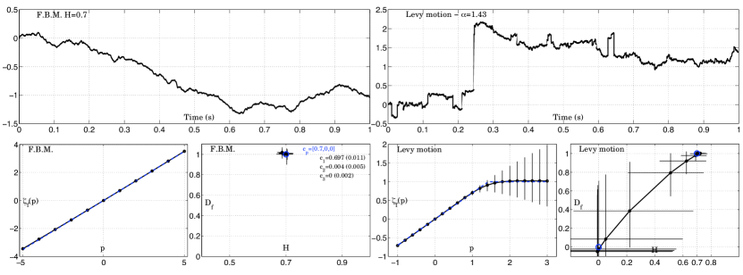
Figure 2: Selfsimilar processes. Top row: sample paths of fBm with $H=0.7$ (left) and of stable Lévy motion with $H=0.7$ (right). Bottom row: estimated wavelet leader scaling functions and Legendre spectra. Both processes have leader scaling functions that behave linearly in $p$ for $p$ close to $0$: $\zeta_{f}(p)=pH$ for fBm, $\zeta_{f}(p)=Hp$ (if $p$ is close to 0) for stable Lévy motion. These self similar processes with stationary increments are thus characterized by $c_{2}=0$. While fBm shows a linear in $p$ leader scaling function and is mono-Hölder, stable Lévy motion is multifractal and its leader scaling function is only piecewise linear (cf. discussion in Section 5.4). Confidence intervals are constructed based on the non parametric bootstrap procedure described in [183].

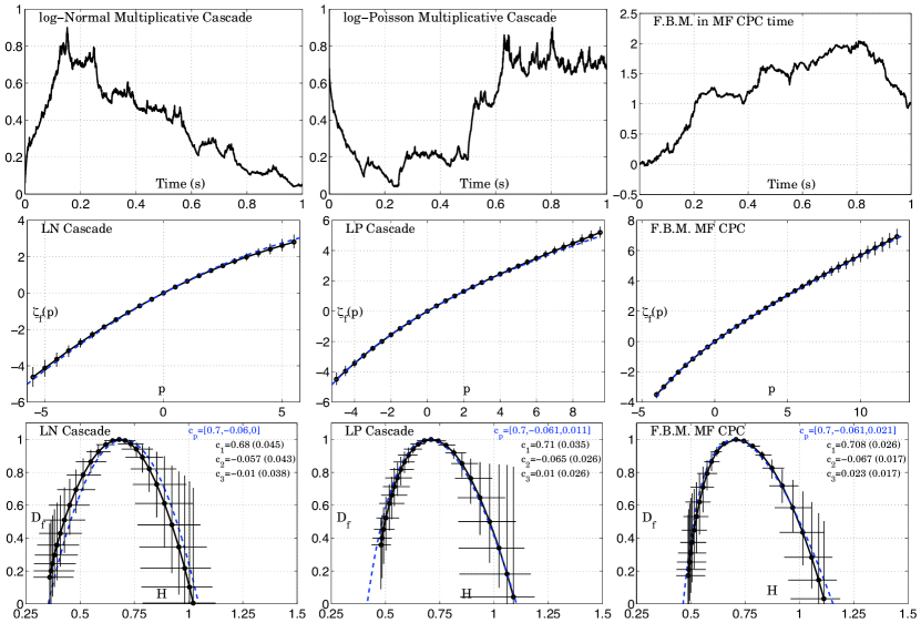
Figure 3: 1D multifractal processes. Top row: sample paths of log-normal cascade (left), log-Poisson cascade (middle), and a fBm in multifractal time (as defined in (51)) (right). 2nd and 3rd rows show the superimposition of the theoretical (blue) and estimated (black) corresponding leader scaling functions and multifractal spectra. Theory and estimation are strikingly in agreement both for positive and negative $p$s and across the entire multifractal spectra (increasing and decreasing parts). Confidence intervals are obtained by a non parametric bootstrap procedure described in [183].

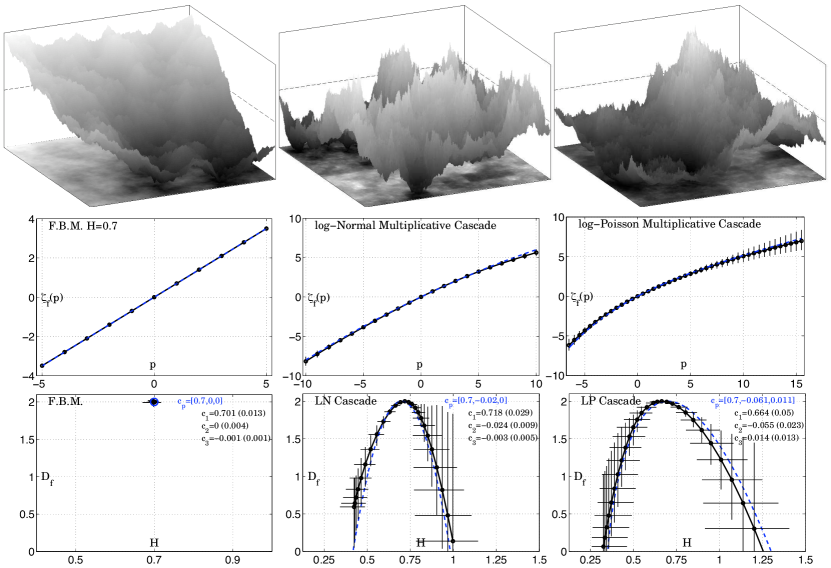
Figure 4: 2D multifractal processes. Top row: 2D realizations of fBm (left), log-normal cascade (middle), log-Poisson cascade (right). 2nd and 3rd rows show the superimposition of the theoretical (blue) and estimated (black) corresponding leader scaling functions and multifractal spectra. As in the 1D case (cf. Figs. 2 and 3), theory and estimates are strikingly in agreement both for positive and negative $p$s and across the entire multifractal spectra (increasing and decreasing parts). Confidence interval are constructed using a non parametric bootstrap procedure described in [183].

The following relationship holds for most standard models used in multifractal analysis:

$${h^{min}_{f}}=\inf(supp(D_{f})).$$ (45)

Note however that this relationship is not true in all generality; for instance the “chirp”

$$F_{\alpha,\beta}(x)=|x|^{\alpha}\sin\left(\frac{1}{|x|^{\beta}}\right)$$

(for $\alpha$ and $\beta$ positive) satisfies

$$h^{min}_{F_{\alpha,\beta}}=\frac{\alpha}{\beta+1}\hskip 8.53581pt\mbox{and }\hskip 8.53581pt\inf\left(supp\left(D_{F_{\alpha,\beta}}\right)\right)=\alpha.$$

However, we will mention a partial result confirming (45) in Section 5.3.

5.3 Local spectrum and homogeneity

So far, little attention has been paid to the region where multifractal analysis is performed, implicitly assuming that it is conducted on the entire set of data available. However, one may wonder whether multifractal analysis would yield different results when applied to different domains. The answer is often negative: Scaling functions, and spectra of singularities, when measured on a sub-part of the data (say a non-empty open subset, in order to dismiss boundary problems) do not depend on the particular open set which is chosen. When such is the case, the function analyzed is said to have homogeneous multifractal properties. It is observed that large categories of experimental data have homogeneous multifractal properties: It is for instance the case for fully developed turbulence, where analyses performed on different parts of the signal always yield the same results. However, this might not systematically be the case.

A simple cause of non-homogeneity can be that data consist of a juxtaposition of different pieces, concatenated together. This situation is commonly met in image processing: Indeed, because of occlusion effects (i.e. objects in the front of the picture partly mask objects behind), images usually appear as a patchwork of homogeneous textures. In this case, it is reasonable to isolate the different components of the data, and perform multifractal analysis over each piece independently. Scaling functions computed on the whole image simply result as the minimum of the local scaling functions, and conversely the global multifractal spectrum consists of the maximum of the local spectra. Note that such cases can lead to simple examples of (global) non-validity of the multifractal formalism. Indeed, the scaling function of the whole image remains, by construction, a concave function, whereas the spectrum, as a maximum of concave function needs no more be concave, even if each component is. Therefore, the multifractal formalism will fail, since, by construction, the right hand side of (42) always yields concave functions.

However, more intricate situations may exist, where multifractal characteristics can evolve with time (or the location, for images) in a way which is more involved than piecewise constant. One can expect, for instance, that stock market data display different statistics during different market phases, such as crises or bubbles. Different multifractal characteristics could stem from such differences. One may also expect that the whole conditions of economy evolve with time, as a consequence of the ever increasing complexity of financial operations, of new financial products, and (more subtly) of mathematical models which themselves influence the way that operators react to the market; all this pleads for possible smooth (or not so smooth) modifications of multifractal characteristics with time. Such possible mechanisms may help to interpret the empirical observations that multifractal properties of market price fluctuations, such as those reported in Fig. 7 (bottom row plots) for the hourly Euro-USD rate, are significantly changing along time (cf. Section 6.2 for discussion).

On the mathematical side, such situations have been barely studied so far (see a contrario the results concerning heterogeneous ubiquity, by J. Barral, A. Durand and S. Seuret, where sophisticated mathematical tools have been developed to deal with the theoretical challenges of this situation [34, 33, 35, 62]). A typical example, studied in [27], is supplied by Markov processes (i.e. processes with independent increment) which do not have stationary increments (and thus are not Lévy processes). Roughly speaking, such processes have jumps of random amplitude, but each jump brings the process in a new environment, and the local multifractal properties will depend on this environment which is randomly chosen. One therefore obtains a non-homogeneous process, with a random spectrum, and random scaling functions. To the opposite, homogeneous multifractals have some additional regularity properties. For instance, the pitfall mentioned in the previous subsection does not occur: An homogeneous multifractal function satisfies (45). An interesting phenomenon of homogeneity breaking will be discussed in the next subsection: We will consider a homogeneous monohölder stochastic process, whose square is not homogeneous, and no longer monohölder.

Note also that a test for the constancy along time of the multifractal properties measured using the leader scaling function and relying on a non parametric bootstrap procedure was proposed in [182].

5.4 Mono vs. Multifractality?

Disentangling issues.  For practical purposes, it is often of interest to decide whether data are mono- or multifractal. However, despite apparent simplicity, as such the question is ill-posed and can be rephrased in different ways:

1. Are data characterized by a single Hölder exponent that takes the same and unique value everywhere or do there exist a variety of Hölder exponents in data?

2. Are data better described by a selfsimilar process (often implicitly meaning fBm) or by a cascade based process? In this later formulation, the important underlying question is: Is there an additive (as in random walk and hence selfsimilar models) or a multiplicative (as in cascades) structure underlying data and hence revealing significant differences in the nature of the data.

3. Are the scaling exponents (i.e., the scaling function) measured on data linear in $p$ or not?

Relying on the fBm (Gaussian based) intuition, these three different formulations are often thought to be equivalent. This section aims at discussing some of the subtleties underlying the relations between these three questions.

Log-cumulants.  Recall that, if they exist, the cumulants of a random variable $X$ are the coefficients of the Taylor expansion of the second characteristic function of $X$, i.e. the coefficients $c_{m}$ (if they exist) in the expansions

$$\log\left({\hbox{I\kern-1.99997pt\hbox{E}}}\left(e^{pX}\right)\right)=\sum_{m=1}^{\infty}c_{m}\frac{p^{m}}{n!}.$$ (46)

Following [44, 46, 58], the cumulants of the log of the wavelet leaders are now introduced. Let $C_{m}(j)$ denote the $m$-th order cumulant of the random variables $\log(d_{j,k})$. Under stationarity and ergodicity assumptions on this sequence, $C_{1}(j)$ is the expectation of the $\log(d_{j,k})$, $C_{2}(j)$ their variance, etc. Assuming that the moments of order $p$ of the leader $d_{j,k}$ exist, starting from the assumption ${\hbox{I\kern-1.99997pt\hbox{E}}}(d_{j,k}^{p})={\hbox{I\kern-1.99997pt\hbox{E}}}(d_{0,0}^{p})\cdot 2^{-j\zeta_{f}(p)}$, one obtains that

$$\log({\hbox{I\kern-1.99997pt\hbox{E}}}(d_{j,k}^{p}))=\log({\hbox{I\kern-1.99997pt\hbox{E}}}(d_{0,0}^{p}))+\zeta_{f}(p)\log(2^{-j});$$

using (46), one obtains the following expansion for $p$ close to $0$:

$$\log({\hbox{I\kern-1.99997pt\hbox{E}}}(d_{j,k}^{p}))=\log({\hbox{I\kern-1.99997pt\hbox{E}}}(e^{p\log d_{j,k}}))=\sum_{m\geq 1}C_{m}(j)\frac{p^{m}}{m!}.$$

Comparing these two expansions, we obtain that the $C_{m}(j)$ are necessarily of the form

$$C_{m}(j)=C^{0}_{m}+c_{m}\log(2^{-j}),$$ (47)

and that $\zeta_{f}(p)$ can be expanded around $0$ as

$$\zeta_{f}(p)=\sum_{m\geq 1}c_{m}\frac{p^{m}}{m!}.$$ (48)

The concavity of $\zeta_{f}$ implies that $c_{2}\leq 0$. Note that, even if the moment of order $p$ of $d_{j,k}$ is not finite, the cumulant of order $m$ of $\log(d_{j,k})$ is likely to be finite and (47) above is also likely to hold. Moreover, (47) provides practitioners with a direct way to estimate the $c_{m}$ by means of linear regressions in $C_{m}(j)$ versus $\log(2^{-j})$ diagrams [183]. The $c_{m}$ are hence not derived from an a posteriori expansion performed from the estimates of the $\zeta_{f}(p)$, but instead estimated directly. For the sake of completeness, let us mention that the polynomial expansion of $\zeta_{f}(p)$ around $0$ can be translated, via the Legendre transform, into an expansion of $L_{f}(h)$ around its maximum [181], on condition that $c_{2}\neq 0$:

$$L_{f}(h)=d+\frac{c_{2}}{2!}\left(\frac{h-{c_{1}}}{c_{2}}\right)^{2}+\frac{-{c_{3}}}{3!}\left(\frac{h-{c_{1}}}{{c_{2}}}\right)^{3}+\frac{-{c_{4}}+3{c_{3}}^{2}/{c_{2}}}{4!}\left(\frac{h-{c_{1}}}{{c_{2}}}\right)^{4}+\ldots$$ (49)

Mono vs. Multi-Hölder.  The only general mathematical result concerning the validity of the multifractal formalism is supplied by Theorem 1, which, in general does not yield the spectrum. However, it does yield an interval in which the support of the spectrum is included: Indeed, let

$${h^{min}_{f}}=\inf\{h:L_{f}(h)\geq 0\}\hskip 14.22636pt\mbox{ and}\hskip 14.22636pth_{f}^{max}=\sup\{h:L_{f}(h)\geq 0\}.$$

Then, the support of the spectrum $D_{f}(h)$ is included in the interval $[{h^{min}_{f}},h_{f}^{max}]$. (It can indeed be checked that ${h^{min}_{f}}$ thus defined actually coincides with the uniform Hölder exponent, defined in Section 4.3.) An important particular case stems from the situation where ${h^{min}_{f}}$ and $h_{f}^{max}$ coincide, in which case the spectrum is supported by the sole point ${h^{min}_{f}}=h_{f}^{max}$, so that only one single Hölder exponent exists in the data, which therefore constitute a monohölder function satisfying

$$\forall x,\hskip 17.07164pth_{f}(x)={h^{min}_{f}}=h_{f}^{max}.$$

This puts into light the necessity to use both positive and negative values of $p$ in the estimation: If the leader scaling function was determined only for positive $p$, the upper bound supplied by Theorem 1 would yield an increasing function, and therefore would, at best, yield the increasing part of the spectrum. In particular, $h_{f}^{max}$ would not be obtained, hence preventing from drawing any conclusion with respect to data being monohölder or not.

However, testing the theoretical equality ${h^{min}_{f}}=h_{f}^{max}$ is practically difficult as the estimation of these quantities turns out to be poor (cf. e.g., [183, 185]). Instead, one can estimate the parameter $c_{2}$ as defined above in (47). When the estimated $c_{2}$ is found strictly negative, this unambiguously indicates multi-Hölder function. As discussed below, the converse is however not necessarily true: $c_{2}=0$ does not necessarily imply monohölder function, as may be incorrectly extrapolated from the Gaussian fBm case.

Let us also note that both approaches based on multifractal analysis can be regarded as non parametric: Testing for mono- or multi-Hölder can be achieved without recourse to any parametric setting, in sharp contradistinction with other existing estimators (for example, many estimators evaluate the selfsimilarity index $H$ assuming that the data are sample paths of an fBm).

Estimated $c_{2}$ measured on real-world data are reported in Section 6: Turbulence velocity is well-known as the emblematic real-world example where a non vanishing parameter $c_{2}$ is met, (cf. Section 6.1, Fig. 6). This is observed to be also the case for the Euro-USD price fluctuations (cf. Section 6.2 and Fig. 7, bottom row, left plot) and for fetal heart rate variability (cf. Section 6.3 Fig. 8). However, Internet traffic aggregated count time series are found to be characterized by $c_{2}=0$ at coarse scales and weakly departing from $0$ at fine scales (cf. Section 6.4 and Figs. 10 and 11, bottom row, left plots).

Selfsimilarity?  Selfsimilar processes are often obtained as renormalized limits of random walks (see for instance the fBm, or stable Lévy processes). Because of the additive structure underlying their nature, selfsimilar models are appealing for describing data. From the examples shown in Section 5.2, it can even be conjectured that scaling functions often are piecewise linear functions. In particular, combining ergodicity and stationarity properties, the Kolmogorov scaling function of selfsimilar processes with stationary increments should behave linearly in $p$, as $\eta_{f}(p)=pH$ on an interval of $p$ containing $0$ (where $H$ is the selfsimilarity parameter). Conjecturing that this property also holds for $\zeta_{f}(p)$, it follows that testing for selfsimilarity can be formulated as testing for $c_{2}=0$. This has been conducted in a non parametric bootstrap framework, cf. e.g., [182, 183]. Note, however, that selfsimilarity with stationary increments together with $c_{2}=0$ does not imply mono-Hölder sample paths (cf. the example of Levy motion reported in Section 5.2 above). Furthermore, $c_{2}=0$ indicates selfsimilarity but does not necessarily imply that data follow a fBm model. This would in addition require to test for joint Gaussianity of all finite distribution functions.

Non linear point transform.  Let us give some further insights into the relevance of the question of deciding whether data are mono or multi-Hölder. We aim at showing that the notion of monoHölder function is, in some sense, unstable since it can be altered under the action of the most simple smooth non-linear operator. To that end, let us consider fBm $B_{H}(t)$, which is the simplest example of a mono-Hölder stochastic process: The Hölder exponent is everywhere equal to $h=H$. Let us now further consider its square transform $Y_{H}(t)=(B_{H}(t))^{2}$. On one hand, at points where the sample path of fBm does not vanish, the action of the mapping $x\rightarrow x^{2}$ locally acts as a $C^{\infty}$ diffeomorphism, and the pointwise regularity is therefore preserved. On other hand, consider now the (random) set $A$ of points where fBm vanishes. The uniform modulus of continuity of fBm implies that a.s., for $s$ small enough,

$$\sup_{t}|B_{H}(t+s)-B_{H}(t)|\leq C|s|^{H}\sqrt{\log(1/|s|)}.$$

therefore, if $B$ vanishes at $t$, then $B_{H}(t+s)^{2}\leq C|s|^{2H}\log(1/|s|)$, so that $h_{Y}(t)\geq 2H$. The converse estimate follows from the fact that, for every $t$,

$$\limsup_{s\rightarrow 0}\frac{|B_{H}(t+s)-B_{H}(t)|}{|s|^{H}}\geq 1,$$

so that, if $B_{H}(t)=0$, then

$$\limsup_{s\rightarrow 0}\frac{(B_{H}(t+s))^{2}}{|s|^{2H}}\geq 1,$$

so that $h_{Y}(t)\leq 2H$. Thus, at vanishing points of $B_{H}$, the action of the square is to shift the Hölder exponent from $h=H$ to $h=2H$. This set of points has been the subject of investigations by probabilists (cf. the flourishing literature on the local time either of Brownian motion, or of fBm); in particular, it is known to be a fractal set of dimension $1-H$, cf [145]. It follows that $Y_{H}(t)$ is a bi-Hölder process, whose spectrum is given by

$$D_{Y_{H}}(h)=\left\{\begin{array}[]{lll}1&\mbox{ if}&h=H,\\ 1-H&\mbox{ if}&h=2H,\\ -\infty&\mbox{ elsewhere.}&\end{array}\right.$$ (50)

Because the multifractal formalism yields the Legendre transform, i.e., the concave hull, of the multifractal spectrum, the leader based estimated multifractal spectrum would suggest practitioners to (wrongly) conclude that $Y_{H}(t)$ is a fully multifractal function whose spectrum is supported by the interval $[H,2H]$. This is illustrated in Fig 5 where it can be observed that the leader based measured multifractal spectrum yields a very precise estimation of the exact concave hull of $D_{Y_{H}}(h)$. Again, note that this is made possible only because negative values of $p$ can be used in the leader framework.

Further, the analysis of the $y=x^{2}$ point transform of fBm raises another disturbing issue. The multifractal properties of fBm are homogeneous (i.e., the spectrum measured from a restriction of the sample path to any interval $(a,b)$ on the real line is the same as that corresponding to the whole one). This is no longer true for $(B_{H})^{2}$: the spectrum measured on a restricted interval $(a,b)$ will vary depending on whether the interval includes or not a point where $B_{H}$ vanishes. This example shows that the multifractal properties are not preserved under simple non linear transformations.

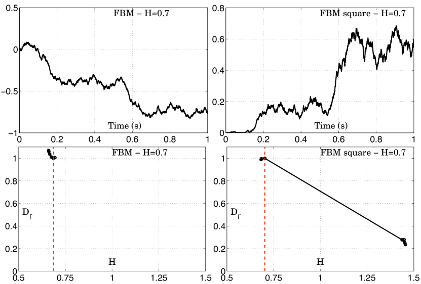
Figure 5: Non linear transform. Top row: sample path of fBm, with $H=0.7$ (left) and its squared transform (right). Bottom row: estimated wavelet leader based Legendre spectra. fBm is a mono-Hölder process and its estimated Legendre spectrum collapses on the theoretical spectrum $D(h)=1$ for $h=H$. Its squared non linear point transform, however, is a bi-Hölder process, with theoretical multifractal spectrum given in (50): The estimated Legendre spectrum perfectly reproduces its corresponding concave hull.

6 Real-World Applications

Reviewing the literature dedicated to real-world applications reveals that the concepts of scaling, scale invariance, selfsimilarity, fractal geometry and multifractal analysis have been and continue to be used to analyze data in numerous contexts of very different natures, ranging from natural phenomena — physics (hydrodynamic turbulence [76, 124, 144], astrophysics and stellar plasmas [174], statistical physics [25, 104], roughness of surfaces [15]), biology (human heart rate variabilities [86, 87, 110, 119, 117], fMRI [53, 81], physiological signals or images), geology (fault repartition, [73]) — to human activities — computer network traffic [152], texture image analysis [15], population geographical repartition [57, 74], social behaviors or financial markets [42, 157]. B. Mandelbrot himself significantly contributed to the studies of many different applications, two of the most prominent possibly being hydrodynamic turbulence, the scientific field that actually gave birth to the essence of multifractal, (cf. e.g., [124, 132]) and finance (cf. e.g., [21, 22, 43, 135]).

As a tribute to B. Mandelbrot’s outstanding research work, a small number of applications from widely different origins have been selected to be revisited. Their presentations are not intended as state-of-the-art reviews, but rather as illustrations, both of the theoretical arguments developed in the previous sections and of the benefits obtained from using multifractal analysis in these applications.

6.1 Hydrodynamic Turbulence

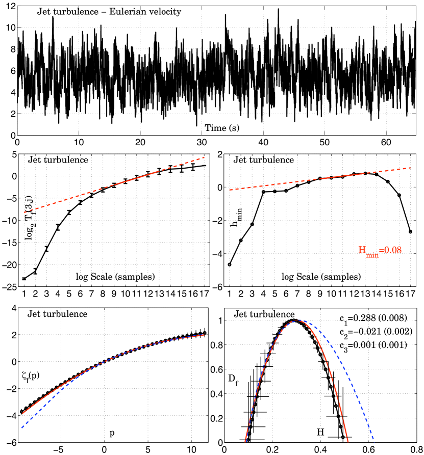
Figure 6: Hydrodynamic Turbulence. Top: longitudinal Eulerian turbulence velocity signal (hot-wire anemometry, Reynolds number: $\simeq 500$, Courtesy C. Baudet et al. [50])). Middle: log-log plot for the wavelet leader based $T_{f}(3,j)$ (as in (39)) and for the wavelet coefficients based ${h^{min}_{f}}$ (as in (37)). Bottom: Wavelet leader scaling function (left) and multifractal spectrum (right) measured from a single run of data (black solid lines), compared to the log-normal (red solid lines) and log-Poisson (dashed blue lines) models. Data clearly select the log-normal model.

In the early $20$s, Richardson, combining empirical observations with the analysis of Navier-Stokes equations, that mostly govern fluid flows, formulated a heuristic description of the apparently random movements observed in hydrodynamic turbulence flows, in terms of a cascade of energy: Between a coarse scale (where energy is injected by an external forcing) and a fine scale (where energy is dissipated by viscous friction), no characteristic scale can be identified. This seminal contribution paved the road to tremendous amounts of works involving the concept of scaling to model turbulence flows (cf. [76, 144] for ancient and modern reviews, respectively). In 1941, Kolmogorov proposed a non explicit version of fBm to model velocity (which implies that $c_{1}=H$, and $c_{m}\equiv 0$ for $m\geq 2$) [106]. However, a general consensus (a rare situation worth mentioning for the field of turbulence) amongst practitioners conducting real experiments rejected fBm as a valid model because the empirically observed scaling exponents (Kolomogorov scaling function) did not behave linearly in $p$, for $p\geq 0$. Framed in seminal contributions due to A. Yaglom [186] and supported by physical arguments developed by Kolmogorov (and his collaborator A. Obukhov) in 1962 [108, 149], the energy transfer from coarse to fine scales has been modeled via split/multiply iterative random procedures that account for the physical intuitions beyond the vorticity stretching mechanisms implied by the Navier-Stokes equation. In 1974, B. Mandelbrot studied these various declinations of cascades and their properties [124], paving the way for their interpretation as a collection of singularities and hence to the first formulation of the multifractal formalism by G. Parisi and U. Frisch, based on the Kolmogorov scaling function [151].

This work triggered enourmous amounts of analysis of experimental and real-world turbulence data, aiming at measuring as precisely as possible scaling exponents (i.e., the scaling function). The earliest contributions relied on the Kolmogorov scaling function (cf. e.g. [16, 14, 45, 47, 51, 158]), and later work initiated by A. Arneodo, E. Bacry and J.-F. Muzy relied on the use of wavelets (cf. e.g. [58, 114, 142, 146, 147, 183]).

Fig. 6 (top plot) shows an example of a turbulence longitudinal Eulerian velocity signal, measured with hot-wire anemometry techniques. It has been collected on a jet turbulence experiment [50], at average Reynolds number $\simeq 580$, and has been made available to us by C. Baudet and collaborators (LEGI, Université Joseph Fourier, INPG, CNRS, Grenoble, France), who are gratefully acknowledged. Middle row plots depict its scaling property in the so-called inertial range, a priori defined from the physical characteristics of the flow conditions: Left, the wavelet leader based $\log_{2}T_{f}(j,q)$ versus $\log_{2}2^{j}$ (for $p=3$), and ${h^{min}_{f}}$ on the right. In the bottom row the measured wavelet leader scaling function and multifractal spectrum are plotted, clearly indicating multifractality.

While the generic multifractality of turbulence data (understood as a strict departure from linearity in $p$ of the scaling function) has never been called into question by any of these studies, a major open issue remains: Which precise cascade model better describes turbulence? This question is not purely theoretical, since the precise ingredients entering the cascade that best match data may reveal physical mechanisms of importance for turbulence. Two such models are emblematic of this issue: In 1962, Obukhov and Kolmogorov [108, 149] proposed a model mostly based on a law of large numbers argument and referred to as the log-normal multifractal model. It predicts that $\zeta_{f}(p)=c_{1}p+c_{2}p^{2}/2$ and hence that $c_{m}\equiv 0$ for $m\geq 3$. In 1994, She and Lévêque [172] proposed an alternative construction based on the key ingredient that energy dissipation gradients must remain finite within turbulence flows. It is referred to as the log-Poisson model and yields a multifractal process with all non zero $c_{m}$s.

Fig. 6 (bottom plots) compares the scaling function (left) and multifractal spectrum (right) measured from data (solid black), together with bootstrap based confidence intervals (cf. [183] for details) against those predicted by the log-normal (solid red) and log-Poisson (dashed blue) model. Together with the fact that the measured $c_{3}$ can not be distinguished from $0$ ($c_{3}=0.001\pm 0.001$), these plots clearly indicate that the log-normal model is preferred by turbulence data. This has been studied systematically and on larger data sets in [114, 183] and unambiguously confirms earlier findings reported in [14, 58].

6.2 Finance Time Series: Euro-USD rate fluctuations

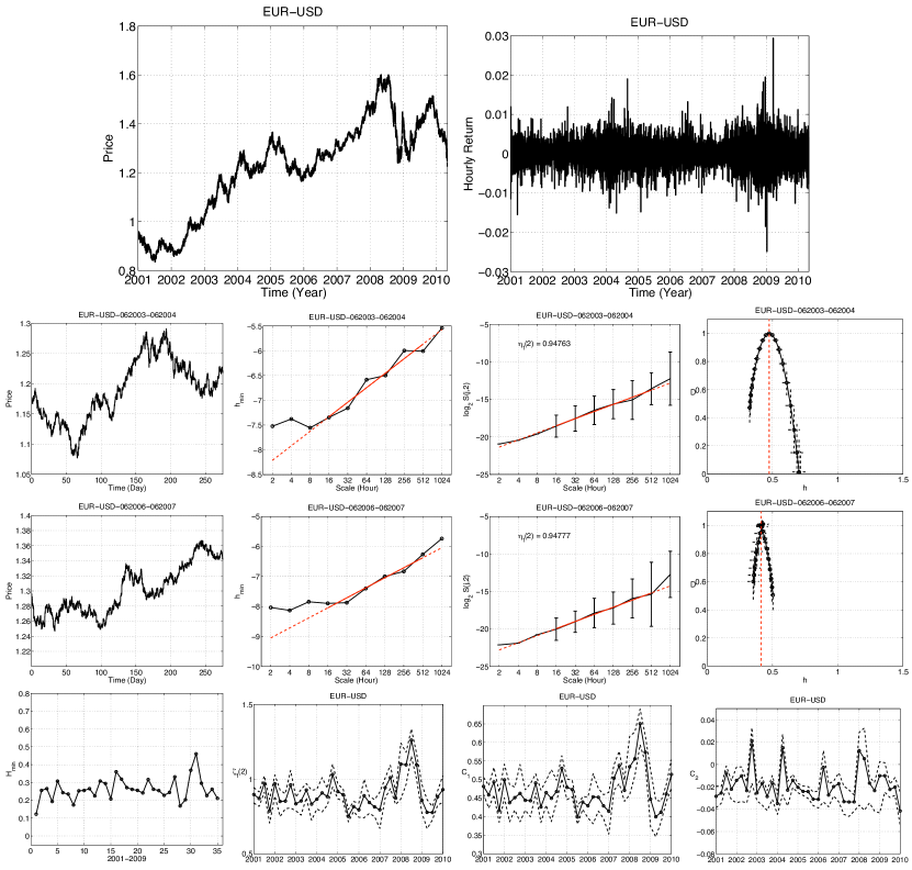
Figure 7: Euro-USD. Top: Euro-USD rate fluctuations for 10 years (starting January 1st, 2001) (left) and hourly returns (right). Data Courtesy Vivienne Investissement, Lyon, France. One year long time series (June 2003 to June 2004, 2nd row; June 2006 to June 2007, 3rd row), with log-log plots for the wavelet coefficients based ${h^{min}_{f}}$ (cf. (37)), log-log plots for the wavelet leader based $T_{f}(2,j)$ (given by (39)), and multifractal spectra, measured using the wavelet leader multifractal formalism. Bottom row: Estimation in one year long time windows (with a $3$-month sliding shift) of ${h^{min}_{f}}$, $\eta_{f}(2)$, $c_{1}$, $c_{2}$ (together with confidence intervals). These plots show that while ${h^{min}_{f}}>0$, $\zeta_{f}(2)$ often remains below the finite quadratic variations limit of $1$. Parameter $c_{1}$, $c_{2}$ variations indicate that the multifractal properties of the Euro-USD price fluctuations vary significantly along time.

Modeling stock market prices received considerable efforts and attention starting with the seminal early contribution of Bachelier in 1900 who, in his thesis, based his description of stock market on Brownian motion, i.e., on an ordinary Gaussian random walk [18]. Essentially, this model implies that daily returns, i.e., increments of (or differences between) prices taken along two consecutive days, $X(t)=P(t)-P(t-1)$, consist of independent, identically distributed Gaussian zero-mean random variables. This hence leaves little room to earn money from stock market investments by pure statistical model based prediction. However, it has long been observed and/or expected that stock market prices significantly depart from the Brownian model: First, returns may exhibit statistics that significantly depart from Gaussian distributions. Second, it is often observed that volatility, a quantity essentially based on the squared (or absolute) value of the returns, display some form of dependency. Notably, in their celebrated contribution, Granger and Joyeux indicated that volatility is well characterized by long memory, or long term dependence [78, 79], a model that is closely related with selfsimilarity and fBm. This motivated substantial efforts to model stock market returns with the GARCH models family or FARIMA alternatives (cf. e.g., [36, 60, 178]).

B. Mandelbrot significantly contributed to the analysis of the statistical properties of stock market returns by performing an iconoclastic analysis of commonly used finance models, emphasizing heavy tails, as opposed to Gaussian distributions (the Noah effect), and long memory, as opposed to independence (the Joseph effect), cf. [133] for a review, and several seminal contributions of B. Mandelbrot; see also e.g., [121, 122]. In particular, this called into question the Black and Scholes model strongly relying on Gaussianity, and led B. Mandelbrot and collaborators to explicitly propose that stock market prices may have multifractal properties in [70] in contradistinction with most Itô-martingale based models used so far. B. Mandelbrot’s work paved the way towards numerous efforts to assess multifractality empirically in stock market prices and exploit it (cf. e.g., [20, 21, 41, 42, 157]).

Almost one century after Bachelier, B. Mandelbrot and collaborators proposed a new model for stock market prices: fBm in multifractal time [43, 135], a process that explicitly incorporates multifractal properties by a multifractal time jittering, obtained by a multiplicative cascade construction. In this model, a new generation of cascades is used, based on Compound Poisson distributions, following again an original idea of B. Mandelbrot [29, 30, 31]. Let $F$ denote the distribution function of the multiplicative cascade $\mu$ on $[0,1]$: $F(t)=\mu([0,t)).$ Then, fBm in multifractal time is defined as

$$X_{t}=B_{H}(F(t)),$$ (51)

where $B_{H}$ stands for fBm with selfsimilarity parameter $H$ (which is independent of $\mu$). Note that, as a consequence of (20), the spectrum of $X$ is deduced from the spectrum of $F$ by a simple dilation along the $h$ axis

$$D_{X}(h)=D_{F}(h/H);$$

see the results of R. Riedi and S. Seuret [165, 171] for additional discussions concerning multifractal subordination, i.e. understanding multifractal properties of composed processes). Numerous rich and interesting declinations of such constructions of cascades and multifractal processes have been proposed since (cf. e.g., [19, 20, 21, 23, 24, 42, 48, 49]). Note that the idea of multifractal subordination (i.e., composition by a multifractal change of time) is extremely powerful, and can be applied in many settings. Let us mention just one example: In [101], B. Mandelbrot and one of the authors performed the multifractal analysis of the Polya function (a famous example of continuous space-filling function) by simply remarking that it can be factorized as the composition of the repartition function of a simple dyadic cascade with a monohölder function.

As a tribute to B. Mandelbrot’s contributions, though the authors have not personally contributed to the field, the multifractal properties of the Foreign exchange Euro-USD price fluctuations are now studied. Fig. 7 (top row) shows the hourly Euro-USD quotations (and hourly returns) since the birth of Euro (Data Courtesy Vivienne Investissement, Lyon, France, /www.vivienne-investissement.com/). The return (or increment) time series clearly shows large fluctuations that are not consistent with a constant along time Gaussian distribution. Scaling properties analyzed here are found to hold for scales ranging from the day to the month, and hence correspond to long term characteristics, as opposed to intra-day analysis, not conducted here. Multifractal spectra measured over one year long time series (second and third rows, left plots), using the wavelet leader multifractal formalism, show that the Euro-USD quotations exhibit multifractal spectra that are in agreement with the fBm in multifractal time model, yet indicate that the multifractal properties may vary along the years. To further analyze these variations, scaling attributes are measured in one year long time windows (with a $3$-month sliding time shift) and reported (together with confidence intervals) in Fig. 7 (bottom row). Interestingly, it is found that ${h^{min}_{f}}$ is permanently above $0$: ${h^{min}_{f}}>0$, which clearly rules out the use of jump processes to model ForEx time series. Moreover, because ${h^{min}_{f}}>0$, the finiteness of quadratic variations can be evaluated using the leader scaling function at $p=2$, $\zeta_{f}(2)$ (as in (39), cf. Section 4.4). Fig. 7 (bottom row, 2nd plot) shows that $\zeta_{f}(2)$ fluctuates and often remains below the finite quadratic variations limit of $1$: $\zeta_{f}(2)<1$. This result validates the hypothesis of the finiteness of quadratic variations, underlying the use of Itô-martingale processes as models to describe the Euro-USD variations, at least when long term variations are analyzed, as is the case here; this does not exclude that shorter term (or intra-day) variations might show different properties. In Fig. 7 (bottom row, 3rd and 4th plots), parameters $c_{1}$, $c_{2}$ are plotted as functions of time. These plots furthermore indicate that though a fBm in multifractal time-like process provides a valid model to describe the price fluctuations, the multifractal properties may vary along time. Two different regimes are suggested by these plots: Before 2007, with a $c_{1}\simeq 0.45<0.5$ and $c_{2}\simeq-0.02$ ; and after 2008, with $c_{1}\simeq 0.5$ and $c_{2}\simeq-0.01$. Recalling that the ordinary Brownian motion (proposed by Bachelier) would correspond to $c_{1}=0.5$ and $c_{2}=0$, it may be concluded that the (long term) fluctuations of the Euro-USD quotations show less structure for the later period than for the former, hence making predictions for investments more difficult (see also discussion in Section 5.3 on homogeneous multifractal properties).

Assuming that the fBm in multifractal time model studied by L. Calvet, A. Fisher and B. Mandelbrot is the correct description of prices, let us now show how the parameter $H$ of the corresponding fBm can be inferred from the observed data using the wavelet scaling function (the heuristic argument that follows can easily be turned into a mathematical proof). Let us first return to the definition of the Kolmogorov scaling function (8). Approximating the integral by a Riemann sum, and taking $h=2^{-j}$, one obtains

$$\int|X_{t+h}-X_{t}|^{p}dt\sim 2^{-j}\sum_{k}\left|X_{\frac{k+1}{2^{j}}}-X_{\frac{k}{2^{j}}}\right|^{p}=2^{-j}\displaystyle\sum_{k}\left|B_{H}\left(F\left({\frac{k+1}{2^{j}}}\right)\right)-B_{H}\left(F\left({\frac{k}{2^{j}}}\right)\right)\right|^{p}$$

which, using the fact that $|B_{H}(t)-B_{H}(s)|\sim|t-s|^{H}$, is of the order of magnitude of

$$2^{-j}\sum_{k}\left|F\left({\frac{k+1}{2^{j}}}\right)-F\left({\frac{k}{2^{j}}}\right)\right|^{pH}.$$

In particular, for $p=1/H$, using the fact that $F$ is continuous and increasing, we obtain

$$2^{-j}\sum_{k}\left|F\left({\frac{k+1}{2^{j}}}\right)-F\left({\frac{k}{2^{j}}}\right)\right|=2^{-j}\sum_{k}\left(F\left({\frac{k+1}{2^{j}}}\right)-F\left({\frac{k}{2^{j}}}\right)\right)=2^{-j}$$

Since this quantity is, by definition, of the order of magnitude of $(2^{-j})^{\eta_{f}(p)}$, we obtain that the exponent $H$ of the fBm used in this model (cf. [43]) satisfies

$$\eta_{f}\left(\frac{1}{H}\right)=1.$$ (52)

Using the fact that the Kolmogorov and the wavelet scaling function coincide in the range of exponents involved here, (52) allows to recover the selfsimilarity exponent of the fBm in this model from the wavelet scaling function. In the example considered in Fig. 7, one obtains that, in practice, the parameter $H$ thus estimated is very close to $c_{1}$.

6.3 Fetal Heart Rate Variability

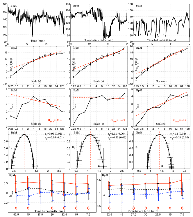
Figure 8: Fetal-ECG. Top: Examples of cardiac frequency time series (in Beats-per-Minute) for fetuses during delivery process - last $15$ min. before delivery, for a healthy subject, correctly diagnosed as such by the obstetrician (left) (True Negative), for a healthy subject, incorrectly diagnosed as suffering from per partum asphyxia (middle) (False Positive), for a fetus actually suffering from per partum asphyixia and diagnosed as such (True Positive). Data Courtesy M. Doret, Obstetrics Dept. of the University Hospital Femme-Mère-Enfant, Lyon, France. Second Row: log-log plots for the wavelet leader based $T_{f}(2,j)$ (cf. (39)). Third Row: log-log plots for the wavelet coefficients based ${h^{min}_{f}}$ (as in (37)). Fourth Row: Multifractal spectra, measured using the wavelet leader multifractal formalism. Bottom Row: Parameters ${h^{min}_{f}}$ (left) and $c_{1}$ (right) estimated over $15$ min. long sliding windows (with a $7.5$min overlap) over the last hour before delivery, values are averaged over the classes of $15$ patients each: True Positive (dashed blue line with ’o’), False Positive (dashed black line with squares, True Positive (solid red line with $\ast$). The red $\diamond$ correspond to windows where a Wilcoxon ranksum test between True Positive and True Negative gives a $p-$value below $5\%$. This analysis shows that unhealthy subjects (True Positive) systematically display less HRV as compared to healthy ones (True Positive and False Positive) (cf. [9, 61]).

Heart rate variability (HRV), which refers to the short time fluctuations (within the minute) of heart rate, has long been considered as a powerful tool to characterize the health status of a given subject: In a nutshell, the more variability, the healthier the subject is (cf. e.g., the seminal contribution [10]). To characterize variability in heart rate time series, spectral analysis has long been used to measure the so called LF/HF balance, i.e., the ratio of energies measured in frequency bands attached to the sympathic and parasympathic activities of the autonomous central nervous system [10]. Yet, it has long been observed that heart rate time series display fractal properties and that the corresponding fractal exponent could be used as a non invasive tool for non healthy status detection (cf. [10]). This opened the way to numerous analyses aiming at describing HRV data with fBm-like models and at correctly estimating the corresponding selfsimilarity parameter $H$; later, multifractal analysis has naturally been considered as an analysis tool potentially improving the characterization of HRV scaling properties (cf. e.g., [86, 87, 110]). Recently, multifractal analysis has been involved in the detection of per partum fetal asphyxia. Obstetricians are monitoring fetal-HRV during the delivery process to detect potential fetal asphyxia. Using a set of analysis criteria (the international FIGO rules), obstetricians measure the health status of the fetus and decide on operative delivery or not. A major difficulty they are facing is the high number of False Positive (fetuses diagnosed as unhealthy during the delivery process but a posteriori evaluated as perfectly healthy), and hence of operative delivery that might have been avoided. This constitutes an important public health issue, as operative deliveries are accompanied by a significant number of serious posterior complications for both newborns and their mothers.

Fig. 8 (top row) shows examples of heart rate time series (in Beats-per-Minute) for a healthy subject, correctly diagnosed as such by the obstetrician (left) (True Negative), for a healthy subject, incorrectly diagnosed as suffering from per partum asphyxia (False Positive), and for a fetus actually suffering form per partum asphyixia and diagnosed as such (True Positive). Data Courtesy M. Doret, Obstetrics Dept. of the University Hospital Femme-Mère-Enfant, Lyon, France, [9, 61]. As shown in Fig. 8 (second and third rows), for all three classes (True Negative, True Positive, False Positive), HRV exhibits scaling properties for scales ranging from the second to the minute. The fourth row in Fig. 8 shows multifractal spectra, estimated from $15$ min. long heart rate time series using wavelet leaders, which suggests that the healthier the subject, the larger its variability in the sense that its $c_{1}$ parameter is smaller (spectrum shifted to the left). To confirm such an observation, multifractal parameters are estimated within $15$ min. long sliding windows (with a $50\%$ time overlap) for the last hour before delivery. The $15$ min. window duration is chosen after the obstetrician’s request that asphyxia should be detected as early as possible. Multifractal parameters are then averaged within the three classes (each containing $15$ patients carefully selected as representative by obstetricians). A Wilcoxon ranksum test is conducted for each time window between the True Positive and False Positive classes. The results reported in Fig. 8 (bottom row) clearly indicate a significant increase of $c_{1}$ and ${h^{min}_{f}}$ (hence a significant decrease in HRV) for the Unhealthy True Positives compared to the Healthy True Negatives and False Positives. The p-value of the Wilcoxon ranksum test is observed to be below $5\%$ (cf. red $\diamond$ in Fig. 8 (bottom row)) often $30$ min earlier than the time the decision to operate the delivery was actually taken. These promising results are reported in details in [9, 61] and will be further investigated.

It is worth noting that for heart rate time series (as for many other types of human rhythms signals, cf. e.g., fMRI applications [53, 81]), ${h^{min}_{f}}$ can be found either positive or negative depending on the subject, or its health status. This is consistent with the fact that practitioners, in applications, noticed that they often had to switch from fBm to fGn (or conversely) to model data and understood this as a puzzling inconsistency (see for instance discussions in [81]). To some extent, the general framework developed here alleviates such inconsistency by introducing ${h^{min}_{f}}$ as one of the various parameters that can be used to analyze scaling without a priori assumptions on the data. In the analysis of fetal HRV described above, a fractional integration of order $1/2$ (larger than the absolute value of the most negative ${h^{min}_{f}}$ encountered in the whole database) has been applied to enable the use of the wavelet leader multifractal formalism in a consistent manner on the whole set of data.

6.4 Aggregated Internet Traffic

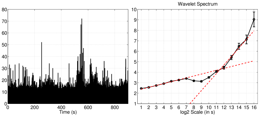
Figure 9: Internet Traffic: Aggregated time series and scaling. Left: Aggregrated time series (Courtesy MAWI research project, [141]); Right: log-log plot for the wavelet coefficient based $S_{f}(2,j)$ (as in (34)). It clearly displays two independent scaling ranges, below and above the second.

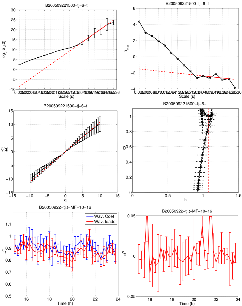
Figure 10: Internet Traffic: Coarse scales. Top: log-log plots for the wavelet leader based $T_{f}(2,j)$ (cf. (39)) (left) and for the wavelet coefficients based ${h^{min}_{f}}$ (as in (37)) (right). Middle: Wavelet leader scaling function (left) and multifractal spectrum (right) measured from $15$-min long data. Bottom: Evolution along time of parameters $c_{1}$ (left) and $c_{2}$ (right), measured from $15$-min long sliding windows for $24$ consecutive hours ($9$ hours shown here; cf. [39]), suggesting that scaling properties are constant along time and clearly validating that, at coarse scales, i.e., above $1$s, aggregated Internet traffic are selfsimilar with long memory ($c_{1}\simeq H\simeq 0.9$) and show no multifractality ($c_{2}\simeq 0$).

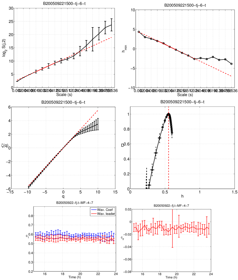
Figure 11: Internet Traffic: Fine Scales. Top: log-log plots for the wavelet leader based $T_{f}(2,j)$ (as in (39)) (left) and for the wavelet coefficients based ${h^{min}_{f}}$ (given by (37)) (right). Middle: Wavelet leader scaling function (left) and multifractal spectrum (right) measured from $15$-min long data. Bottom: Evolution along time of parameters $c_{1}$ (left) and $c_{2}$ (right), measured from $15$-min long sliding windows for $24$ consecutive hours ($9$ hours shown here). (cf. [39]), also suggest that scaling properties are constant along time and indicate that, at fine scales (i.e., below $1$s), aggregated Internet traffic are characterized by $c_{1}\simeq H\simeq 0.6$ and $c_{2}\simeq 0.005\pm 0.005$, revealing at best a very weak multifractality or no multifractality at all.

Internet traffic engineering currently is a challenging task involving a variety of issues ranging from economy development planning and security assessment to statistical data characterization. The earliest versions of statistical models used for Internet traffic modeling were stemming from the experience gained on the previous large communication network: Telephone communications. B. Mandelbrot himself made very early contributions to such modeling (cf. e.g., [37]), and this certainly was a major source of inspiration for the later developments he made in the theory of fractal stochastic processes. However, such telephone communications models were all based on the assumption that there exist one or several characteristic scales of time in data, while it has soon been recognized that Internet traffic is well characterized by long memory and self similarity (cf. [8, 115, 116, 153, 154] for seminal articles). This later raised the question of multifractality of Internet traffic (cf. e.g., [1, 69, 84, 166]) that we briefly illustrate here.

Any activity performed on the net (emailing, web browsing, Video-On-Demand, data downloading, IP telephony,…) amounts to establishing a connection between hosts (server-clients, peer to peer, …), consisting of computers located all over the world, according to an agreed-on protocol, and exchanging a (very) large number of elementary quanta of information, the Internet Protocol packets (in short, IP Pkts). Collecting Internet traffic data hence naturally consists of recording the IP Pkt time stamp and header (IP source, IP destination, Port Source, Port Destination). Obviously, analyzing the marked point process resulting of the tremendous number of IP Pkts exchanged is beyond feasible, and it is classical to instead monitor so-called aggregated (or count) time series: Practitioners select a given aggregation-level $\Delta$, whose choice depends on the application, and construct either the Pkt or Byte time series that counts the number of IP Pkts whose timestamp falls within $[k\Delta,(k+1)\Delta)$, or the corresponding volume in Byte.

An example of such Pkt time series is plotted in Fig. 9 (left). It consists of traffic from the MAWI repository, made available by the Japanese WIDE research program [141]. The MAWI repository consists of data that have been collected everyday for $15$min at $2$ pm (Tokyo time) since January 2001 on major backbone links ($100$Mbps or $1$Gbps) connecting Japan and the United States (cf. [39, 52, 59].

The left plot of the same figure displays the wavelet coefficient based $\log_{2}(S_{f}(2,j))$ vs. $\log_{2}(2^{j})=j$ (as in (34)) and clearly shows that, for Internet traffic, there exist two ranges of scales for which scaling can be identified: Coarse scales, above $1$s, and fine scales, below $1$s. For each of those ranges of scales, the wavelet leader based multifractal formalism is applied.

For the coarse scales, Fig. 10 clearly indicates on a $15$min long set of data aggregated at $1$ms that the leader scaling function is linear, and that the multifractal spectrum collapses on a single point, hence suggesting monofractality or that multifractality is at best very weak. To further investigate this point, the parameters $c_{1}$ and $c_{2}$ are estimated on sliding $15$min long windows for a trace collected during $24$ hours (on Sept., 22nd, 2005), for scales ranging from $1$s to $1$ min. Results are reported for the last $8$ hours for simplicity and show, first, that the estimated parameters are remarkably constant along the day (while the changes in amplitude of the time series may be drastic) and, second, that $c_{2}\simeq 0$. This indicates no multifractality at coarse scale and, because $c_{1}\sim H\simeq 0.9$, a significant long memory in the data. These experimental results corroborate those reported in [84] and are consistent with the main model due to Taqqu et al. (cf. [176]) relating selfsimilarity and heavy-tails of the web file size distribution, see also [2, 83, 118]).

For the fine scales, Fig. 11 shows on the same $15$min long set of data aggregated at $1$ms that the leader scaling function is linear for $p$ around $0$, hence indicating a very weak multifractality or no multifractality at all. Parameters $c_{1}$ and $c_{2}$, estimated on sliding $15$min long windows for the $24$ hour trace, again turn out to be constant along time, with $c_{1}\simeq 0.55\pm 0.05$ and $c_{2}\simeq 0.007\pm 0.005$. This hence validates that fine scales of aggregated traffic show at best little multifractality. Furthermore, estimations of the selfsimilarity parameters (not shown here) being close to $0.5$ also indicate little correlation. These analyses tend to show that fine scales of aggregated traffic are characterized by the quasi-absence of dependence structure. Moreover, the estimated parameters $c_{1}$ and $c_{2}$ remain remarkably constant along time for the whole day and across the various days analyzed, a highly unexpected result for Internet traffic, which is often described as widely varying, and which is continuously subject to numerous occurrences of anomalies and attacks. This is essentially because data have been pre-processed using a random projection and a median procedure that robustify estimation against anomalous behaviors (cf. [39, 59]). In practice, the effect of this procedure is to eliminate abnormal components in the traffic. The results reported here can hence be associated with the properties of regular and legitimate background Internet traffic, corresponding to the usual Internet user behaviors. Furthermore, this quasi-absence of dependence structure at fine scales is consistent with the Cluster Point Process modeling of Internet traffic aggregated count time series proposed in [84], which implies that fine scales are actually not possessing strictly scaling properties. However, it also shows that the statistical properties of the fine scales are satisfactorily approximated by scaling behaviours. Therefore, the fact that regular or legitimate traffic does not show multifractality does not imply however that multifractal parameters like $c_{1}$ and $c_{2}$ can not be used for traffic monitoring, such as anomaly detection for instance. Indeed, the occurrence of anomalies is likely to change the dependence structure of the fine scale statistics (as shown in e.g., [59]) and consequently the empirically estimated parameters $c_{1}$ and $c_{2}$, which may thus prove very useful, even if scaling properties are measured that actually consist of approximations of the true statistical properties of the fine scales.

Finally, let us mention that for aggregated count time series ${h^{min}_{f}}<0$, as shown on the top left plots of Figs. 10 and 11, hence a fractional integration of order $1$ is systematically applied prior to performing the wavelet leader multifractal formalism.

6.5 Texture classification: Vincent Van Gogh meets Benoît Mandelbrot

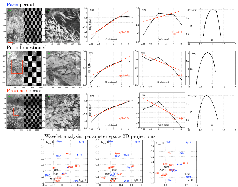
Figure 12: Van Gogh’s Paintings. Left columns: Representative examples of paintings of the Paris (top), Provence (bottom) and unknown (middle) periods, with selected homogeneous patches (second column), Courtesy Image Processing for Art Investigation research program, cf. www.digitalpaintinganalysis.org/, and the Van Gogh and Kröller-Müller Museums (The Netherlands). Third column: log-log plots for the wavelet coefficient based $S_{f}(1,j)$ (as in (34)). Fourth column: ${h^{min}_{f}}$. Right column: Wavelet leader based multifractal spectra, suggesting that the questioned painting has multifractal properties close to that of the Provence period example. Bottom row: 2D projections of multifractal attributes, indicating that paintings from the Paris period (blue) are overall globally more regular than paintings from the Provence period (red).

Applications described so far all implied the multifractal analysis of 1D signals only. However, B. Mandelbrot always advocated that fractal analysis should be applied to images, to characterize the roughness of textures (cf. e.g., [125, 126]). The wavelet coefficient based analysis of selfsimilarity analysis has been readily and immediately extended to 2D fields and images, thanks to the straightforward formulation of the 2D discrete wavelet transform (cf. e.g., [120]). The estimation of the corresponding $H$ parameter has then been used to characterize textures in images, often in the context of biomedical applications (cf. [38, 97]). The extension of multifractal formalisms to images turned out to be significantly more intricate. Direct extension of the Kolmogorov scaling function were used to analyze rainfall repartitions by D. Schertzer and S. Lovejoy, see [169]. A second attempt based on the modulus maxima of the coefficients of the 2D continuous wavelet transform was proposed by A. Arneodo and his collaborators; it employed in medical [13] or geophysical applications [15]. The wavelet leader formalism recently proposed and based on a 2D discrete wavelet transform enabled a significant step forward toward the use of multifractal analysis in higher dimensions. Its potential benefits have been assessed in [184], and it has recently been used to characterize texture in paintings [6].

The paintings that Van Gogh performed while he was living in France are grouped into two periods by art experts and art historians: The Paris period, ending early 1888, and the later Provence period. While art experts agree on the classification of most of Van Gogh’s paintings, some are still not clearly attributed to either period. To perform such classification, art experts often make use of material or stylometric features such as the density of brush strokes, their size or scale, the thickness of contour lines, the layers, the chemicals of the colors, ….

Aiming at promoting the investigation of computer-based image processing procedures to assist art experts in their judgement, the Image Processing for Art Investigation research program (cf. www.digitalpaintinganalysis.org/), in collaboration with the Van Gogh and Kröller-Müller Museums (The Netherlands), made available to research teams two sets of (partial and low resolution digitized versions of) $8$ Van Gogh’s paintings each from the Paris and Provence period, and $3$ painting whose period remains undecided (nomenclature below corresponds to the Van Gogh museum catalog). The digitized copies are available through the usual RGB (Red, Blue, Green) channels and converted into the HSV (Hue, Saturation, Value) channels, hence enabling to process the gray-level light intensity information and the color information.

Three examples, corresponding to the Paris period, the Provence period and unclassified paintings, respectively, are shown in Fig. 12 (left column) together with examples of homogenous patches selected for analysis (second column). The 2D wavelet leader based multifractal formalism has been applied, for each selected patch, independently to the six RGB and HSV channels. Examples of obtained multifractal spectra are shown in Fig. 12 (right column) and suggest, for example, that $f605$ is closer to $f475$ than to $f452$ and hence is likely to belong to the Provence period. For each patch of the $2\times 8+3$ paintings and each channel, multifractal attributes ${h^{min}_{f}},\eta_{f}(1),c_{1},\dots$ are estimated. Fig. 12 (bottom row) shows 2D projections of various pairs of such attributes, which all indicate that on average the Paris paintings (blue clusters) are globally more regular than the Provence paintings (red clusters). Also, the Saturation and Red channels are found to be the most discriminant. This suggests that both a color and an intensity information (saturation and Red) are useful for discrimination. Interestingly, it has been reported by art experts that saturation is a key feature to distinguish between the Paris and Provence periods in Van Gogh’s paintings. Finally, these 2D projections suggest that $f605$ and $f386$ belong to the lower left red cluster and hence to the Provence period, while conclusion is less straightforward for $f572$. Such results are left to the appreciation of art experts. These analyses are detailed in [6].

7 Conclusion

A key issue for the future developments of multifractal analysis is to disentangle (at least) four different acceptations that can be associated with the key word multifractal, and that are often misleadingly confused one with another, sometimes leading to potential misunderstandings and erroneous interpretations.

Theoretical multifractal analysis and local regularity.  From the theoretical or mathematical side, multifractal analysis is deeply tied with the analysis of the fluctuations along time (or space) of the local regularity of the function or data of interest, these fluctuations being often coined as irregularity. Usually, this local regularity is measured in terms of Hölder exponents $h_{f}(x)$. The global description of the irregularity of $f$ is gathered in the multifractal spectrum $D_{f}(h)$, which consists of the Hausdorf dimensions of the geometrical iso-Hölder sets. For mathematics, multifractal is hence all about Hölder exponent and (fractal, or box or Haussdorf) dimensions of geometrical sets. Though listed first here, the mathematical formulation of multifractal analysis theory can be considered as the most recent piece of the history of multifractal, as it really started in the 90s only, see [40], as a consequence of the seminal article of G. Parisi and U. Frisch [151]. Note however that precursors can be found, for instance in articles dealing with slow and fast points of Brownian motion: Recall that this specific process displays exceptional points where the modulus of continuity is slightly smaller (resp. bigger) than a.e.; the corresponding sets are random fractals. Following the seminal contribution of J.-P. Kahane, their dimensions have been precisely determined, respectively by S. Orey and S. J. Taylor for fast points, see [150], and by E. Perkins for slow points, see [156].

Multifractal formalism and scale invariance.  From the more practical perspective of real-world data analysis, scaling functions, consisting of time (or space) averages of the $p$-th power of scale dependent quantities (such as increments, oscillations, wavelet coefficients or wavelet leaders) — also often referred to, in statistical physics, as partition or structure functions — constitute the core aspect of the notion of multifractal. Importantly, practical multifractal analysis amounts in essence to assuming that scaling functions behave as power laws with respect to the analysis scales, in the range of scales available in the data. The description of these power laws naturally leads to the notion of scaling exponents. Equivalently, these scaling exponents are termed scaling functions, with the practical and often implicit request that the limit underlying its definition actually exists (cf. (8) versus (9)).

These power law behaviors — or scale invariance, or scaling — of scale dependent quantities, and the corresponding scaling exponents (or scaling functions), were at the heart of the intuition that B. Mandelbrot developed, connecting scaling properties to (fractal) dimensions, to selfsimilarity and/or to fluctuations of local regularity, and relating scaling to self similar random walks or multiplicative cascades.

The multifractal formalism (in reference to the Thermodynamic formalism) therefore consists of the mathematical developments that relate scale invariance and scaling functions to local regularity and multifractal spectra. In some sense, the multifractal spectrum constitutes the link between formal mathematics and physics or data analysis.

Multifractal processes.  Multifractal processes do not constitute a well-defined class. In essence, this notion refers to processes (or functions) that can be fruitfully used to model scale invariance properties in data. Following the seminal distinctions proposed by B. Mandelbrot, they can be thought of as falling into two major classes: Selfsimilar random walks and multiplicative cascades (or martingales).

The first one, now very classical after the seminal review of B. Mandelbrot on fBm [138], pertains to the class of additive models: A large step (or increment) can be obtained as the sum of many different small steps, yet sharing the same statistical properties. This class is hence deeply associated with selfsimilarity. Often, this class is confused with its emblematic but restrictive representative fBm, the only Gaussian selfsimilar process with stationary increments. The Gaussian nature of this process and its fully parametrized formulation lead to the formulation of various parametric estimation of its selfsimilarity exponent $H$. Such parametric estimation are sometimes incorrectly considered as a multifractal analysis of data. This is inaccurate since multifractal analysis aims at measuring much richer properties of data than the sole selfsimilarity and, above all, does not rely on the assumption that data are selfsimilar or Gaussian. Multifractal analysis thus has a much broader scope and can also be applied to limits of other random walks, such as Lévy processes (and, more generally, jump processes), see [26] for overviews on the mathematical side.

The second class, multiplicative cascades, is usually considered as that of archetypal multifractal processes, in the sense that their (scaling functions and) multifractal spectra can be computed theoretically and found to often consist of continuous, smooth bell-shaped functions. Therefore, for such processes, multifractal analysis unveils information that can not easily be obtained with other analysis tools (as opposed to the previous class of selfsimilar random walks).

Furthermore, as mentioned earlier, and again following one of B. Mandelbrot’s intuitions, this particular class can be extended by combinations (or subordinations) of selfsimilar process with multiplicative cascades (for instance fBm in multifractal time mentioned above, or Lévy processes in multifractal time, as studied by J. Barral and S. Seuret [33, 34]).

It is however clear that these examples do not even give a vague idea of the tremendous variety of all possible multifractal functions. A few mathematical results actually comfort this idea (and allow to transform it into a precise mathematical statement): Generically, most functions in a given function space are multifractal and satisfy the multifractal formalism, see [75, 92] for precise statements. Therefore, multifractality is not a rare property, and is certainly not restricted to the few examples which have been investigated up to now.

The classical opposition between monofractal versus multifractal processes, often used in practical data analysis, is not well grounded and somehow irrelevant. Confusion stems from the fact that Gaussian fBm is characterized by a single Hölder parameter $h_{f}(x)=H$ and is hence monohölder (its spectrum $D_{f}(h)$ is supported by a single point). But selfsimilarity does not in general imply this monohölder property. Instead, the classification of data might be by opposing additive to multiplicative structure. Indeed, the physics (or the biology or else) underlying data production may significantly differ depending on whether it is driven by additive mechanisms, or by multiplicative ones. In that respect, multifractal analysis may help as the multifractal spectra of selfsimilar random walks generally differ from those of multiplicative constructions. However, in opposition to what is often used in applications, multifractal analysis per se, understood as the measurement of the scaling function and multifractal spectrum, is not sufficient for proving that there exist any additive or multiplicative structures underlying the data. Multifractal analysis does not aim at stating definite answers to fuzzy questions such as: Are data following a cascade model or not? but, instead, it provides quantitative answers to more restricted questions such as: Is ${h^{min}_{f}}>0$? Is $\zeta_{f}(2)>1$? In turns, these precise measurements can contribute to help practitioners to formulate hypotheses regarding data, or to classify them.

Practical multifractal analysis: signal and image processing.  As stated in the previous paragraph, practical multifractal analysis amounts to measuring from data multifractal attributes such as $\eta_{f}(p),{h^{min}_{f}},\zeta_{f}(p),c_{m},L_{f}(h)$. These quantities can be computed from data without assuming any a priori data model. In other words, data to which multifractal analysis is applied need not stem from any exact selfsimilar random walk or multiplicative construction. Multifractal analysis is hence, by nature, a non parametric analysis tool that can be applied to any type of data, be they (multi)fractal or not. Whether $L_{f}(h)$ can be related with $D_{f}(h)$ or not does not prevent practitioners to use these multifractal attributes as tools for classification, diagnosis, detection, or else. This is notably the case in image processing, where it is very unlikely that databases containing images of widely different natures can be associated with specific construction models (such as random walks or cascades).

Furthermore, in practice, one question is always central and was already raised by B. Mandelbrot: What multiresolution quantity should one start with? Increments, oscillations, wavelet coefficients, wavelet leaders? In this respect, the present contribution aims at providing clear and general answers. First, increments and oscillations only address the restricted case where $0\leq h_{f}(t)<1,\forall t$; while wavelet based quantities enable to bypass that restriction by selecting smooth enough wavelets with a large enough number of vanishing moments. Therefore, wavelet coefficients generalize increments and the wavelet leaders constitute the generalized counterpart of oscillations. Second, wavelet coefficients and wavelet leaders should not be opposed. Wavelet coefficients enable to measure information in data such as the uniform Hölder exponent and a global selfsimilarity type scaling exponent; they should hence always be applied first to data. Wavelet leaders should be applied next, when relevant (${h^{min}_{f}}>0$) and when seeking for additional and more refined analysis of scaling properties in data, via a full collection of scaling exponents $\zeta_{f}(p)$, or equivalently $c_{m}$, or equivalently $L_{f}(h)$.

Multifractal toolbox.  The practical solutions proposed here in terms of discrete wavelet transform coefficients and leaders are believed to be one of the methods enabling the best practical achievements in terms of combining firm mathematical grounding, satisfactory estimation performance, low implementation and computational costs, robustness and versatility. It can be accompanied with non parametric bootstrap procedures, providing confidence intervals for estimates and hypothesis test procedures. Technical details are reported in [183] and Matlab toolboxes implementing these tools are made publicly available by the authors.

References

- [1] P. Abry, R. Baraniuk, P. Flandrin, R. Riedi, and D. Veitch. Multiscale network traffic analysis, modeling, and inference using wavelets, multifractals, and cascades. IEEE Signal Processing Magazine, 3(19):28–46, May 2002.
- [2] P. Abry, P. Borgnat, F. Ricciato, A. Scherrer, and D. Veitch. Revisiting an old friend: On the observability of the relation between long range dependence and heavy tail. Telecom. Syst., Special Issue on Traffic Modeling, Its Computations and Applications, 43(3-4):147–165, 2009.
- [3] P. Abry, P. Gonçalvès, and P. Flandrin. Wavelets, spectrum estimation and processes, chapter 103. Springer-Verlag, New York, 1995. Wavelets and Statistics, Lecture Notes in Statistics.
- [4] P. Abry, P. Gonçalvès, and J. Lévy-Véhel, editors. Lois d’échelle, fractale et ondelettes, Vol. 1 & 2. Hermès Scientific Publications, 2002.
- [5] P. Abry, S. Jaffard, S.G. Roux, B. Vedel, and H. Wendt. Wavelet decomposition of measures: Application to multifractal analysis of images. In Unexploded ordnance detection and mitigation, J. Byrnes ed. Springer, NATO Science for peace and security, Series B, pages 1–20, 2008.
- [6] P. Abry, S. Jaffard, and H. Wendt. When Van Gogh meets Mandelbrot: Multifractal classification of painting’s texture. preprint, 2011.
- [7] P. Abry, B. Pesquet-Popescu, and M.S. Taqqu. Wavelet based estimators for self similar -stable processes. In Int. Conf. on Signal Proc., 16th World Computer Congress, Beijing, China, August 2000.
- [8] P. Abry and D. Veitch. Wavelet analysis of long-range dependent traffic. IEEE Trans. Info. Theory, 44(1):2–15, 1998.
- [9] P. Abry, H. Wendt, S. Jaffard, H. Helgason, P. Goncalvès, E. Pereira, C. Gharib, P. Gaucherand, and M. Doret. Methodology for multifractal analysis of heart rate variability: From ratio to wavelet leaders. In 32nd Annual International Conference of the IEEE Engineering in Medicine and Biology, Buenos Aires, Argentina, 2010.
- [10] S. Akselrod, D. Gordon, F.A. Ubel, D.C. Shannon, A.C. Berger, and R.J. Cohen. Power spectrum analysis of heart rate fluctuation: a quantitative probe of beat-to-beat cardiovascular control. Science, 213(4504):220–222, 1981.
- [11] A. Arneodo, B. Audit, N. Decoster, J.-F. Muzy, and C. Vaillant. Wavelet-based multifractal formalism: applications to dna sequences, satellite images of the cloud structure and stock market data. The Science of Disasters; A. Bunde, J. Kropp, H.J. Schellnhuber, Eds. (Springer), pages 27–102, 2002.
- [12] A. Arneodo, E. Bacry, and J.F. Muzy. The thermodynamics of fractals revisited with wavelets. Physica A, 213(1-2):232–275, 1995.
- [13] A. Arneodo, N. Decoster, P. Kestener, and S.G. Roux. A wavelet-based method for multifractal image analysis: from theoretical concepts to experimental applications. In P.W. Hawkes, B. Kazan, and T. Mulvey, editors, Advances in Imaging and Electron Physics, volume 126, pages 1–98. Academic Press, 2003.
- [14] A. Arneodo, S. Manneville, and J.F. Muzy. Towards log-normal statistics in high Reynolds number turbulence. Eur. Phys. J. B, 1:129, 1998.
- [15] A. Arneodo, S.G. Roux, and N. Decoster. A wavelet-based method for multifractal analysis of rough surfaces: applications to high-resolution satellite images of cloud structure. ”Experimental Chaos”, AIP Conference Proceeding, 622:80, 2002.
- [16] A. Arneodo et al. Structure functions in turbulence, in various flow configurations, at Reynolds number between 30 and 5000, using extended self-similarity. Europhys. Lett., 34:411–416, 1996.
- [17] J.M. Aubry and S. Jaffard. Random wavelet series. Communications In Mathematical Physics, 227(3):483–514, 2002.
- [18] L. Bachelier. Théorie de la spéculation. Annales de l’École Normale Supérieure, 3(17), 1900.
- [19] E. Bacry, J. Delour, and J.F. Muzy. Multifractal random walk. Phys. Rev. E, 64(2):026103, 2001.
- [20] E. Bacry, L. Duvernet, and J.F. Muzy. Continuous-time skewed multifractal processes as a model for financial returns. International Journal of Theoretical and Applied Finance, 2010.
- [21] E. Bacry, A. Kozhemyak, and J.F. Muzy. Continuous cascade models for asset returns. Journal of Economic Dynamics and Control, 32(1):156–199, 2008.
- [22] E. Bacry, A. Kozhemyak, and J.F. Muzy. Multifractal models for asset prices. Encyclopedia of quantitative finance, Wiley, 2010.
- [23] E. Bacry and J.F. Muzy. Multifractal stationary random measures and multifractal random walks with log-infinitely divisible scaling laws. Phys. Rev. E, 66, 2002.
- [24] E. Bacry and J.F. Muzy. Log-infinitely divisible multifractal processes. Commun. Math. Phys., 236:449–475, 2003.
- [25] V. Bareikis and R. Katilius, editors. Proceedings of the 13th International Conference on Noise in Physical Systems and Fluctuations, Palanga, Lithuania. World Scientific, 1995.
- [26] J. Barral, J. Berestycki, J. Bertoin, A. Fan, B. Haas, S. Jaffard, G. Miermont, and J. Peyrière. Quelques interactions entre analyse, probabilités et fractals. S.M.F., Panoramas et synthèses 32, 2010.
- [27] J. Barral, N. Fournier, S. Jaffard, and S. Seuret. A pure jump Markov process with a random singularity spectrum. Annals of Probability, 38(5):1924–1946, 2010.
- [28] J. Barral and P. Gonçalves. On the estimation of the large deviations spectrum. Journal of Statistical Physics, 144(6):1256–1283, 2011.
- [29] J. Barral, X.O. Jin, and B. Mandelbrot. Uniform convergence for complex [0,1]-martingales. Annals of Applied Probability, 20(4):1205–1218, 2010.
- [30] J. Barral and B. Mandelbrot. Multifractal products of cylindrical pulses. Probability Theory and Related Fields, 124(3):409–430, 2002.
- [31] J. Barral and B. Mandelbrot. Multiplicative products of cylindrical pulses. Probab. Theory Rel., 124:409–430, 2002.
- [32] J. Barral and S. Peyrière. Mandelbrot cascades fabulous fate. (in this volume), 2011.
- [33] J. Barral and S. Seuret. The singularity spectrum of Lévy processes in multifractal time. Adv. Math., 14(1):437–468, 2007.
- [34] J. Barral and S. Seuret. On multifractality and time subordination for continuous functions. Adv. Math., 220(3):936–963, 2009.
- [35] J. Barral and S. Seuret. A localized Jarnik-Besicovich theorem. Adv. Math., 226(4):3191–3215, 2011.
- [36] J. Beran. Statistics for Long-Memory Processes. Chapman & Hall, 1994.
- [37] J.M. Berger and B. Mandelbrot. New model for the clustering of errors on telephone circuits. IBM Journal of Research and Development, 7(3):224–236, 1963.
- [38] H. Biermé and F. Richard. Statistical test for anisotropy for fractional Brownian textures. Applications to full–field digital mammography. J. Math. Imaging Vision, 36(3):227–240, 2010.
- [39] P. Borgnat, G. Dewaele, K. Fukuda, P. Abry, and K. Cho. Seven years and one day: Sketching the evolution of internet traffic. In INFOCOM2009, 2009.
- [40] G. Brown, G. Michon, and J. Peyrière. On the multifractal analysis of measures. Journal of Statistical Physics, 66(3-4):775–790, 1992.
- [41] L. Calvet and A. Fisher. Multifractality in assets returns: theory and evidence. Review of Economics and Statistics, LXXXIV(84):381–406, 2002.
- [42] L. Calvet and A. Fisher. Multifractal volatility: Theory, forecasting and pricing. Academic Press, San Diego, CA, 2008.
- [43] L. Calvet, A. Fisher, and B. Mandelbrot. The multifractal model of asset returns. Cowles Foundation Discussion Papers: 1164, 1997.
- [44] B. Castaing. The temperature of turbulent flows. J. Phys. II, 6:105–114, 1996.
- [45] B. Castaing, Y. Gagne, and E. Hopfinger. Velocity probability density functions of high Reynolds number turbulence. Physica D, 46:177–190, 1990.
- [46] B. Castaing, Y. Gagne, and M. Marchand. Log-similarity for turbulent flows. Physica D, 68(3-4):387–400, 1993.
- [47] B. Castaing, Y. Gagne, and M. Marchand. Log-similarity for turbulent flows. Physica D, 68:387–400, 1993.
- [48] P. Chainais, R. Riedi, and P. Abry. On non scale invariant infinitely divisible cascades. IEEE Trans. Info. Theory, 51(3), March 2005.
- [49] P. Chainais, R. Riedi, and P. Abry. Warped infinitely divisible cascades: beyond scale invariance. Traitement du Signal, 22(1), 2005.
- [50] G.R. Chavarria, C. Baudet, and S. Ciliberto. Hierarchy of the energy dissipation moments in fully developed turbulence. Phys. Rev. Lett., 74:1986–1989, 1995.
- [51] A. Chhabra et al. Direct determination of the singularity spectrum and its application to fully developed turbulence. Phys. rev. A, 40:1327, 1989.
- [52] K. Cho, K. Mitsuya, and A. Kato. Traffic data repository at the wide project. In USENIX 2000 FREENIX Track, 2000.
- [53] P. Ciuciu, P. Abry, C. Rabrait, and H. Wendt. Log wavelet leaders cumulant based multifractal analysis of evi fmri time series: evidence of scaling in ongoing and evoked brain activity. IEEE J. of Selected Topics in Signal Proces., 2(6):929–943, 2009.
- [54] M. Clausel-Lesourd and S. Nicolay. A wavelet characterization for the upper global holder index. Preprint, 2011.
- [55] S. Cohen and J. Istas. Fractional fields and applications. (preprint), 2011.
- [56] I. Daubechies. Orthonormal bases of compactly supported wavelets. Comm. Pure and App. Math., 41:909–996, 1988.
- [57] A. Dauphiné. Géographie fractale. Hermès, Lavoisier, Paris, France, 2011.
- [58] J. Delour, J.F. Muzy, and A. Arneodo. Intermittency of 1d velocity spatial profiles in turbulence: A magnitude cumulant analysis. The Euro. Phys. Jour. B, 23:243–248, 2001.
- [59] G. Dewaele, K. Fukuda, P. Borgnat, P. Abry, and K. Cho. Extracting hidden anomalies using sketch and non Gaussian multiresolution statistical detection procedures. In SIGCOMM 2007 Workshop LSAD - ACM SIGCOMM 2007 Workshop on Large-Scale Attack Defense (LSAD), Kyoto, Japan, 2007.
- [60] I. Dittman and C.W.J. Granger. Properties of nonlinear transformations of fractionally integrated processes. Journal of Econometrics, 110:113–133, 2002.
- [61] M. Doret, H. Helgason, P. Abry, P. Gonçalvès, C. Gharib, and P. Gaucherand. Multifractal analysis of fetal heart rate variability in fetuses with and without severe acidosis during labor. Am. J. Perinatol., 2011. To Appear.
- [62] A. Durand. Random wavelet series based on a tree-indexed Markov chain. Comm. Math. Phys., 283(2):451–477, 2008.
- [63] A. Durand and S. Jaffard. Multifractal analysis of Lévy fields. Proba. Theo. Related Fields (to appear), 2011.
- [64] G.A. Edgar (ed.). Classics on Fractals. Cambridge University Press, 1995.
- [65] P. Embrechts and M. Maejima. Selfsimilar Processes. Princeton University Press, Series in Applied Mathematics, 2001.
- [66] K. Falconer. Fractal Geometry. Wiley, 1990.
- [67] K. Falconer. Fractal Geometry: Mathematical Foundations and Applications. John Wiley & Sons, West Sussex, England, 1993.
- [68] K. Falconer. Techniques in Fractal Geometry. John Wiley & Sons, West Sussex, England, 1997.
- [69] A. Feldmann, A.C. Gilbert, and W. Willinger. Data networks as cascades: Explaining the multifractal nature of internet wan traffic. In SIGCOMM’98, pages 42–55, 1998.
- [70] A. Fisher, L. Calvet, and B. Mandelbrot. Multifractality of Deutsche Mark / US dollar exchange rate. Cowles Foundation Discussion Papers: 1165, 1997.
- [71] P. Flandrin. On the spectrum of fractional Brownian motions. IEEE Trans. Info. Theory, IT-35(1):197–199, 1989.
- [72] P. Flandrin. Wavelet analysis and synthesis of fractional Brownian motions. IEEE Trans. Info. Theory, 38:910–917, 1992.
- [73] E. Foufoula-Georgiou and P. Kumar, editors. Wavelets in Geophysics. Academic Press, San Diego, Calif., 1994.
- [74] P. Frankhauser. L’approche fractale : un nouvel outil dans l’analyse spatiale des agglomerations urbaines. Population, 4:1005–1040, 1997.
- [75] A. Fraysse and S. Jaffard. How smooth is almost every function in a sobolev space? Revista Matematica Iberoamericana, 22(2):663–682, 2006.
- [76] U. Frisch. Turbulence, the Legacy of A.N. Kolmogorov. Addison-Wesley, 1993.
- [77] Y. Gousseau and J.-M. Morel. Are natural images of bounded variation? SIAM J. Math. Anal., 33:634–648, 2001.
- [78] C.W.J. Granger. Long memory relationships and the aggregation of dynamic models. J. of Econometrics, 14:220 – 238, 1980.
- [79] C.W.J. Granger and R. Joyeux. An introduction to long memory time series models and fractional differencing. Journal of Time Series Analysis, 1:15 – 29, 1980.
- [80] T.C. Halsey, M.H. Jensen, L.P. Kadanoff, I. Procaccia, and B.I. Shraiman. Fractal measures and their singularities - the characterization of strange sets. Phys. Rev. A, 33(2):1141–1151, 1986.
- [81] B. He. The temporal structures and functional significance of scal-free brain activity. Neuron, 66:353–369, 2010.
- [82] D. Hernad, M. Mouillard, and D. Strauss-Kahn. Du bon usage de R/S. Revue de Statistique Appliquée, 26(4):61–79, 1978.
- [83] N. Hohn, D. Veitch, and P. Abry. Cluster processes: A natural language for network traffic. IEEE Transactions On Signal Processing, 51:2229–2244, 2003.
- [84] N. Hohn, D. Veitch, and P. Abry. Multifractality in tcp/ip traffic: the case against. Computer Network Journal, 48:293–313, 2005.
- [85] H.E. Hurst. Long-term storage capacity of reservoirs. Transactions of the American Society of Civil Engineering, 116:770–799, 1951.
- [86] P.C. Ivanov. Scale-invariant aspects of cardiac dynamics. IEEE Eng. In Med. and Biol. Mag., 26(6):33–37, 2007.
- [87] P.C. Ivanov, L.A. Nunes Amaral, A.L. Goldberger, S. Havlin, M.G. Rosenblum, Z.R. Struzik, and H.E. Stanley. Multifractality in human heartbeat dynamics. Nature, 399:461–465, 1999.
- [88] S. Jaffard. Multifractal formalism for functions. SIAM J. of Math. Anal., 28(4):944–998, 1997.
- [89] S. Jaffard. Oscillation spaces: Properties and applications to fractal and multifractal functions. Journal of Mathematical Physics, 39(8):4129–4141, 1998.
- [90] S. Jaffard. Sur la dimension de boîte des graphes. Compt. Rend. Acad. Scien., 326:555–560, 1998.
- [91] S. Jaffard. The multifractal nature of Lévy processes. Proba. Theo. Related Fields, 114(2):207–227, 1999.
- [92] S. Jaffard. On the frisch-parisi conjecture. Journal de Mathématiques Pures et Appliquées, 79(6):525–552, 2000.
- [93] S. Jaffard. Wavelet techniques in multifractal analysis. In M. Lapidus and M. van Frankenhuijsen, editors, Fractal Geometry and Applications: A Jubilee of Benoît Mandelbrot, Proc. Symp. Pure Math., volume 72(2), pages 91–152. AMS, 2004.
- [94] S. Jaffard. Beyond Besov spaces, part 2: Oscillation spaces. Constructive Approximation, 21(1):29–61, 2005.
- [95] S. Jaffard. Pointwise regularity associated with function spaces and multifractal analysis. Banach Center Pub. Vol. 72 Approximation and Probability, T. Figiel and A. Kamont, Eds., pages 93–110, 2006.
- [96] S. Jaffard. Wavelet techniques for pointwise regularity. Ann. Fac. Sci. Toul., 15(1):3–33, 2006.
- [97] S. Jaffard, P. Abry, and S.G. Roux. Function spaces vs. scaling functions: tools for image classification. Mathematical Image processing (Springer Proceedings in Mathematics) M. Bergounioux ed., 5:1–39, 2011.
- [98] S. Jaffard, P. Abry, S.G. Roux, B. Vedel, and H. Wendt. The contribution of wavelets in multifractal analysis, pages 51–98. Series in contemporary applied mathematics. World scientific publishing, 2010.
- [99] S. Jaffard, B. Lashermes, and P. Abry. Wavelet leaders in multifractal analysis. In T. Qian, M.I. Vai, and X. Yuesheng, editors, Wavelet Analysis and Applications, pages 219–264, Basel, Switzerland, 2006. Birkhäuser Verlag.
- [100] S. Jaffard, B. Lashermes, and P. Abry. Wavelet leaders in multifractal analysis. In Wavelet Analysis and Applications, T. Qian, M.I. Vai, X. Yuesheng, Eds., pages 219–264, Basel, Switzerland, 2006. Birkhäuser Verlag.
- [101] S. Jaffard and B. Mandelbrot. Peano-polya motion, when time is intrinsic or binomial (uniform or multifractal). The Mathematical Intelligencer, 19(4):21–26, 1997.
- [102] S. Jaffard and C. Melot. Wavelet analysis of fractal boundaries. Communications In Mathematical Physics, 258(3):513–565, 2005.
- [103] J.-P. Kahane and J. Peyrière. Sur certaines martingales de Mandelbrot. Adv. Math., 22:131–145, 1976.
- [104] M. Keshner. noise. Proc. IEEE, 70(3):212–218, 1982.
- [105] A.N. Kolmogorov. The Wiener spiral and some other interesting curves in Hilbert space (russian),. Dokl. Akad. Nauk SSSR, 26:(2):115 118, 1940.
- [106] A.N. Kolmogorov. a) dissipation of energy in the locally isotropic turbulence. b) the local structure of turbulence in incompressible viscous fluid for very large Reynolds number. c) on degeneration of isotropic turbulence in an incompressible viscous liquid. In S.K. Friedlander and L. Topper, editors, Turbulence, Classic papers on statistical theory, pages 151–161. Interscience publishers, 1941.
- [107] A.N. Kolmogorov. The local structure of turbulence in incompressible viscous fluid for very large Reynolds numbers. Comptes Rendus De L’Academie Des Sciences De L’Urss, 30:301–305, 1941.
- [108] A.N. Kolmogorov. A refinement of previous hypotheses concerning the local structure of turbulence in a viscous incompressible fluid at high Reynolds number. J. Fluid Mech., 13:82–85, 1962.
- [109] N. Kôno and M. Maejima. Selfsimilar stable processes with stationary increments. Tokyo J. Math., 14:93–100, 1991.
- [110] K. Kotani, K. Takamasu, L. Safonov, and Y. Yamamoto. Multifractal heart rate dynamics in human cardiovascular model. Proceedings of SPIE, 5110:340–347, 2003.
- [111] S. Osher L. Rudin and E. Fatemi. Nonlinear total variation based noise removal algorithms. Physica D, 60:259–268, 1992.
- [112] B. Lashermes, P. Abry, and P. Chainais. New insight in the estimation of scaling exponents. Int. J. on Wavelets, Multiresolution and Information Processing, 2(4), 2004.
- [113] B. Lashermes, S. Jaffard, and P. Abry. Wavelet leader based multifractal analysis. 2005 Ieee International Conference On Acoustics, Speech, and Signal Processing, Vols 1-5, pages 161–164, 2005.
- [114] B. Lashermes, S.G. Roux, P. Abry, and S. Jaffard. Comprehensive multifractal analysis of turbulent velocity using the wavelet leaders. European Physical Journal B, 61(2):201–215, 2008.
- [115] W.E. Leland, M.S. Taqqu, W. Willinger, and D.V. Wilson. On the self-similar nature of ethernet traffic (extended version). ACM/IEEE Transactions on Networking, 2(1):1–15, February 1994.
- [116] W.E. Leland, M.S. Taqqu, W.Willinger, and D.V. Wilson. On the self-similar nature of ethernet traffic. In SIGCOMM ’93: Conference proceedings on Communications architectures, protocols and applications, pages 183–193, New York, NY, USA, 1993. ACM Press.
- [117] L.S. Liebovitch and A.T. Todorov. Invited editorial on ”fractal dynamics of human gait: stability of long-range correlations in stride interval fluctuations”. J. Appl. Physiol., pages 1446–1447, 1996.
- [118] P. Loiseau, P. Gonçalves, G. Dewaele, P. Borgnat, P. Abry, and P.V. Primet. Investigating self-similarity and heavy-tailed distributions on a large scale experimental facility. IEEE/ACM Transactions on Networking, 18(4):1261–1274, 2010.
- [119] S.B. Lowen and M.C. Teich. Fractal-Based Point Processes. Wiley, Hoboken, NJ, 2005.
- [120] S. Mallat. A Wavelet Tour of Signal Processing. Academic Press, San Diego, CA, 1998.
- [121] B. Mandelbrot. The variation of certain speculative price. The Journal of Business, 36(4):394–419, 1963.
- [122] B. Mandelbrot. Limitations of efficiency and of martingale models. The review of econometrics and statistics, 53(2):225–236, 1971.
- [123] B. Mandelbrot. Possible refinement of the lognormal hypothesis concerning the distribution of energy dissipation in intermittent turbulence, volume 12, pages 333–351. Springer, La Jolla, California, 1972. Statistical Models and Turbulence, Lecture Notes in Physics.
- [124] B. Mandelbrot. Intermittent turbulence in self-similar cascades: divergence of high moments and dimension of the carrier. J. Fluid Mech., 62:331–358, 1974.
- [125] B. Mandelbrot. Geometry of homogeneous scalar turbulence: iso-surface fractal dimensions and . J. Fluid Mech., 72(2):401–416, 1975.
- [126] B. Mandelbrot. Poisson approximation of the multi-temporal Brownian functions and generalizations. Comptes Rendus de l’Académie des Sciences (Paris), 280(A):1075–1078, 1975.
- [127] B. Mandelbrot. Fractals: Form, Chance and Dimension. W. H. Freeman and Company, USA, 1977.
- [128] B. Mandelbrot. The Fractal Geometry of Nature. New York, 1982.
- [129] B. Mandelbrot. Diagonally self-affine fractal cartoons. part 1: Mass, box, and gap fractal dimensions, local or global. Fractals in Physics, pages 3–15, 1985.
- [130] B. Mandelbrot. Diagonally self-affine fractal cartoons. part 2: length and area anomalies. Fractals in Physics, pages 17–20, 1985.
- [131] B. Mandelbrot. Self-affinity and fractal dimension. Physica Scripta, 32:257–260, 1985.
- [132] B. Mandelbrot. Limit lognormal multifractal measures. In E.A. Gotsman et al., editor, Frontiers of Physics, Proc. Landau Memorial Conf., Tel Aviv, 1988, pages 309–340, Oxford, 1990. Pergamon Press.
- [133] B. Mandelbrot. Fractals and scaling in finance. Selected Works of Benoit B. Mandelbrot. Springer-Verlag, New York, 1997. Discontinuity, concentration, risk, Selecta Volume E, With a foreword by R.E. Gomory.
- [134] B. Mandelbrot. Multifractals and noise. Selected Works of Benoit B. Mandelbrot. Springer-Verlag, New York, 1998. Wild Self-Affinity in Physics.
- [135] B. Mandelbrot. A multifractal walk down Wall Street. Sci. Am., 280(2):70–73, 1999.
- [136] B. Mandelbrot. Gaussian Self-Affinity and Fractals. Selected Works of Benoit B. Mandelbrot. Springer-Verlag, New York, 2002.
- [137] B. Mandelbrot. Fractals and Chaos. Selected Works of Benoit B. Mandelbrot. Springer-Verlag, New York, 2004.
- [138] B. Mandelbrot and J.W. van Ness. Fractional Brownian motion, fractional noises and applications. SIAM Reviews, 10:422–437, 1968.
- [139] B. Mandelbrot and W. Wallis. Noah, Joseph, and operational hydrology. Water Resources Research, 4(5):909–918, 1968.
- [140] B. Mandelbrot and W. Wallis. Robustness of the rescaled range R/S in the measurement of noncyclic long run statistical dependence. Water Resources Research, 5(5):967–988, 1969.
- [141] MAWI Traffic Archive. WIDE project. http://mawi.wide.ad.jp/mawi/.
- [142] C. Meneveau. Analysis of turbulence in the orthonormal wavelet representation. J. Fluid Mech., 232:469, 1991.
- [143] Y. Meyer. Ondelettes et Opérateurs. Hermann, Paris, 1990. English translation, Wavelets and operators, Cambridge University Press, 1992.
- [144] A.S. Monin and A.M. Yaglom. Statistical Fluid Mechanics. M.I.T. Press, Cambridge, MA, 1975.
- [145] D. Monrad and L.D. Pitt. Local nondeterminism and Hausdorff dimension. Progress in Probability and Statistics, Seminar on Stochastic Processes 1986, (E. Cinlar, K.L. Chung, R.K. Getoor, Eds.), Birkhäuser, Boston, page 163 189, 1986.
- [146] J.F. Muzy, E. Bacry, and A. Arneodo. Wavelets and multifractal formalism for singular signals: application to turbulence data. Phys. Rev Lett., 67:3515–3518, 1991.
- [147] J.F. Muzy, E. Bacry, and A. Arneodo. The multifractal formalism revisited with wavelets. Int. J. of Bifurcation and Chaos, 4:245–302, 1994.
- [148] E.A. Novikov. Infinitely divisible distributions in turbulence. Phys. Rev. E, 50:R3303–R3305, 1994.
- [149] A.M. Obukhov. Some specific features of atmospheric turbulence. J. Fluid Mech., 13:77–81, 1962.
- [150] S. Orey and S. J. Taylor. How often on a Brownian path does the law of iterated logarithm fail? Proc. London Math. Soc, 28(3):174–192, 1974.
- [151] G. Parisi and U. Frisch. Fully developed turbulence and intermittency. In M. Ghil, R. Benzi, and G. Parisi, editors, Turbulence and Predictability in geophysical Fluid Dynamics and Climate Dynamics, Proc. of Int. School, page 84, Amsterdam, 1985. North-Holland.
- [152] K. Park and W. Willinger. Self-similar network traffic: An overview. In K. Park and W. Willinger, editors, Self-Similar Network Traffic and Performance Evaluation, pages 1–38. Wiley, 2000.
- [153] K. Park and W. Willinger. Self-similar network traffic: An overview. In K. Park and W. Willinger, editors, Self-Similar Network Traffic and Performance Evaluation, pages 1–38, New York, 2000. Wiley.
- [154] V. Paxson and S. Floyd. Wide area traffic: The failure of Poisson modeling. IEEE TON, 4(3):209–223, 1995.
- [155] H.O. Peitgen and D. Saupe, editors. The science of fractal images. Springer-Verlag, 1988.
- [156] E. Perkins. On the Hausdorff dimension of the Brownian slow points. Z. Wahrsch. Verw. Gebiete, 64(3):369–399, 1983.
- [157] E. Peters. Fractal market analysis. Wiley, NYC, USA, 1994.
- [158] S. Pietropinto, C. Poulain, C. Baudet, B. Castaing, B. Chabaud, Y. Gagne, B. Hebral, Y. Ladam, P. Lebrun, O. Pirotte, and P. Roche. Superconducting instrumentation for high Reynolds turbulence experiments with low temperature gaseous helium. Physica C, 386:512–516, 2003.
- [159] V. Pipiras. Wavelet-type expansion of the rosenblatt process. J. Four. Anal. Appli., 10:599?–634, 2004.
- [160] V. Pipiras and P. Abry. Wavelet-based synthesis of the rosenblatt process. Sig. Proc., 86:2326–2339, 2006.
- [161] V. Pipiras and M. Taqqu. Multifractal processes. In P. Doukhan, G. Oppenheim, and M.S. Taqqu, editors, Fractional calculus and its connexions to fractional Brownian motion, pages 165–201. Birkhäuser, 2003.
- [162] V. Pipiras, M.S. Taqqu, and P. Abry. Can continuous-time stationary stable processes have discrete linear representation? Statistics & Probability Letters, 64:147–157, 2003.
- [163] V. Pipiras, M.S. Taqqu, and P. Abry. Bounds for the covariance of functions of infinite variance stable random variables with applications to central limit theorems and wavelet-based estimation. Bernoulli, 13(4):1091–1123, 2007.
- [164] L.F. Richardson. Weather prediction by numerical process. Cambridge University Press, 1922.
- [165] R.H. Riedi. Multifractal processes. In P. Doukhan, G. Oppenheim, and M.S. Taqqu, editors, Theory and applications of long range dependence, pages 625–717. Birkhäuser, 2003.
- [166] R.H. Riedi, M.S. Crouse, V.J. Ribeiro, and R.G. Baraniuk. A multifractal wavelet model with application to network traffic. IEEE Trans. Info. Theory, 45:992–1018, 1999.
- [167] P.-G. Lemarié Rieusset. Distributions dont tous les coefficients d’ondelettes sont nuls. Comptes Rendus Acad. Sci., 318:1083–1086, 1994.
- [168] G. Samorodnitsky and M. Taqqu. Stable non-Gaussian random processes. Chapman and Hall, New York, 1994.
- [169] D. Schertzer and S. Lovejoy. Physically based rain and cloud modeling by anisotropic, multiplicative turbulent cascades. J. Geophys. Res., 92:9693–9714, 1987.
- [170] M. Schroeder. Fractals, Chaos, Power Laws: Minutes from an Infinite Paradise. W.H. Freeman, 1991.
- [171] S. Seuret. On multifractality and time subordination for continuous functions. Adv. Math., 220(3):936–963, 2009.
- [172] Z.S. She and E. Lévêque. Universal scaling laws in fully developed turbulence. Phys. Rev. Letters, 72:336–339, 1994.
- [173] N. R. Shieh and Y. Xiao. Hausdorff and packing dimensions of the images of random fields. Bernoulli, 16 (4):926?–952, 2010.
- [174] J.-L. Starck, F. Murtagh, and A. Bijaoui. Image Processing and Data Analysis: The Multiscale Approach. Cambridge University Press, Cambridge, 1998.
- [175] S. Stoev, V. Pipiras, and M.S. Taqqu. Estimation of the self-similarity parameter in linear fractional stable motion. Signal Processing, 82(12):1873–1901, 2002.
- [176] M.S. Taqqu, W. Willinger, and R. Sherman. Proof of a fundamental result in self-similar traffic modeling. SIGCOMM Comput. Commun. Rev., 27(2):5–23, 1997.
- [177] A.H. Tewfik and M. Kim. Correlation structure of the discrete wavelet coefficients of fractional Brownian motions. IEEE Trans. Info. Theory, IT-38(2):904–909, 1992.
- [178] G. Teyssière and P. Abry. Wavelet analysis of nonlinear long range dependent processes. Applications to financial time series. In Long Memory in Econometrics, G. Teyssière and A. P. Kirman, Eds. Springer, Berlin, 2007.
- [179] D. Veitch and P. Abry. A wavelet-based joint estimator of the parameters of long-range dependence. IEEE Trans. Info. Theory, 45(3):878–897, 1999.
- [180] D. Veitch and P. Abry. A statistical test for the time constancy of scaling exponents. IEEE Trans. Signal Proces., 49(10):2325–2334, 2001.
- [181] H. Wendt. Contributions of Wavelet Leaders and Bootstrap to Multifractal Analysis: Images, Estimation Performance, Dependence Structure and Vanishing Moments. Confidence Intervals and Hypothesis Tests. PhD thesis, Ecole Normale Sup rieure de Lyon, 2008.
- [182] H. Wendt and P. Abry. Bootstrap tests for the time constancy of multifractal attributes. In Proc. IEEE Int. Conf. Acoust., Speech, and Signal Proc. (ICASSP), Las Vegas, USA, 2008.
- [183] H. Wendt, P. Abry, and S. Jaffard. Bootstrap for empirical multifractal analysis. IEEE Signal Processing Mag., 24(4):38–48, 2007.
- [184] H. Wendt, P. Abry, S. Jaffard, H. Ji, and Z. Shen. Wavelet leader multifractal analysis for texture classification. In Proc. IEEE Int. Conf. Image Proc. (ICIP), Cairo, Egypt, 2009.
- [185] H. Wendt, S.G. Roux, P. Abry, and S. Jaffard. Wavelet leaders and bootstrap for multifractal analysis of images. Signal Proces., 89:1100–1114, 2009.
- [186] A.M. Yaglom. Effect of fluctuations in energy dissipation rate on the form of turbulence characteristics in the inertial subrange. Dokl. Akad. Nauk. SSR, 166:49–52, 1966.