Abstract

Recent overwhelming evidences show that the sun strongly influences the Earth’s climate and environment. Moreover existence of life on this Earth mainly depends upon the sun’s energy. Hence, understanding of physics of the sun, especially the thermal, dynamic and magnetic field structures of its interior, is very important. Recently, from the ground and space based observations, it is discovered that sun oscillates near 5 min periodicity in millions of modes. This discovery heralded a new era in solar physics and a separate branch called helioseismology or seismology of the sun has started. Before the advent of helioseismology, sun’s thermal structure of the interior was understood from the evolutionary solution of stellar structure equations that mimicked the present age, mass and radius of the sun. Whereas solution of MHD equations yielded internal dynamics and magnetic field structure of the sun’s interior. In this presentation, I review the thermal, dynamic and magnetic field structures of the sun’s interior as inferred by the helioseismology.

1 Introduction

From the dawn of civilization, sun is revered and held as an awe inspiring celestial object in the sky. In the world, there are many stories and poems woven around the sun god in different folklores and the magnificent architectures are dedicated to the mighty sun. The flora and fauna on the earth mainly depends on the sun for their survival. Recent observational evidences are building up that even the unpredictable climates and rainfalls of the earth are excited and are maintained by the sun’s influence (Reid 1999; Shine 2000; Hiremath and Mandi 2004 and references there in; Soon 2005; Hiremath 2006a, 2006c; Haigh 2007; Perry 2007; Feymann 2007; Tiwari and Ramesh 2007 and references there in; Scafetta and West 2008; Hiremath 2009; Agnihotri, Dutta and Soon 2011). Analysis of vast stretch in time of the paleoclimatic records show that the sun’s activity is imprinted in the global temperature and precipitation variabilities. The imminent influence (Hiremath and Mandi 2004 and references there in; Hiremath 2009 and references there in) of the sun also can be traced in the well documented instrumental rainfall records.

Among all the distant stars, the sun is very closest to us and is apparently $\sim$ 100 billion times brighter than any other star. Thus owing to it’s proximity and brilliance, the sun can be closely studied in details; like it’s chemical composition, thermal and dynamic structures of the interior, etc. The sun is a gigantic cosmic laboratory where one can test the physical phenomena discovered on the earth. Hence the sun is very important astronomical object that needs to be studied carefully. If we understand the sun, we can understand the distant stars and physics of whole universe.

In the recent decade, helioseismology-a tool to probe the solar internal structure and dynamics-has changed our conventional perception of the internal structure and dynamics. Observational evidences show that sun oscillates over a wide range of periods that range from minutes to perhaps on time scales of centuries. Observations from the ground (GONG, BISON, IRIS, etc., ) and from the space (like SOHO, HINODE, STEREO, etc.,) provided solar oscillation frequency data with very high precision.

Before the advent of helioseismology, sun’s internal thermal structure was understood from the standard solar model. A standard solar model is built from the evolutionary calculations of stellar structure equations (conservation of mass, momentum and energy and supplemented with known equation of state, knowledge of transfer of energy by convection in the outer part of the sun, equation of nuclear energy generation and nature of opacity of the solar internal plasma) that ultimately mimic the sun’s present age, mass and radius respectively. As for the dynamical structure, earlier studies concentrated on studying the rotation rate of the solar core as this parameter is related to evolutionary history of angular momentum of the sun and its influence on the orbit of nearby planet Mercury for testing the Einstein’s general theory of relativity.

Similarly, models based on the turbulent $\alpha\omega$ dynamo mechanism required that radial part of the angular velocity should increase from the surface towards the interior in order to reproduce the correct sunspot butterfly diagrams. On the other hand, results of non-linear hydrodynamical simulations (Gilman and Miller 1981) show that angular velocity decreases from the surface towards the interior. These simulations also yield internal rotational isocontours that have cylindrical geometry. However, it will be known from the following sections that the helioseismic inferences yield entirely different picture of the rotational profile in the solar interior. We will also know from the helioseismic inferences and modeling that the thermal structure (such as pressure, temperature, etc.,) of the solar interior is almost similar to the structure obtained from the standard solar model, although recent surface chemical abundances and hence helioseismic inferences yield the substantial disagreement.

Plan of this presentation is as follows. In section 2, a brief introduction to the observational aspects of the sun is presented. Recent discoveries of the sun’s oscillations from the ground and space are presented in section 3. Section 4 is devoted to inferences of thermal, dynamic and magnetic field structures of the sun’s interior. Concluding remarks are presented in the last section. In this presentation, I mainly concentrate on the global seismology to infer global large scale structure of the sun’s interior although one can also infer near surface structure from the local helioseismology.

2 A Brief Observational Introduction to the Sun

Important physical parameters of the sun are : (i) mass-$2\times 10^{30}$ Kg, (ii) radius-$7\times 10^{8}$ meter, (iii) mean density-1409 Kg$m^{-3}$, (iv) temperature at the photosphere-5780 ${}^{o}K$ and, (v) the total amount of energy radiated by the sun (i.e., luminosity) measured at one astronomical unit (i.e., distance between the earth and the sun)-$3.9\times 10^{26}$ joules/sec.

When one considers the vertical cross section of the sun parallel to it’s rotation axis, based on the dynamical and physical properties, solar interior mainly can be classified into three distinct zones : (i) the radiative core where the energy is mainly generated by the nuclear fusion of hydrogen into helium and is transfered by the radiation, (ii) the convection zone where the energy is transferred from the center to the surface by the convection of the plasma and, (iii) the photosphere where the energy is radiated into the space. Above the photosphere, the sun’s atmosphere consists of the chromosphere and the corona. The temperature increases from the layer of photosphere to million degree kelvin in the corona.

If the sun were static in time with a constant output of energy, the planetary environments in general and the earth’s environment in particular would have received the constant output of energy. However, the sun’s energy output is variable due to spatial and temporal variability of the sun’s large scale magnetic field structure, dynamics and flow of mass (both the neutral and charged particles) from the sun. The most outstanding activity of the sun is sunspots- cool and dark features compared to the ambient medium-on the sun’s surface that modulate sun’s irradiance and the galactic cosmic rays that enter the planetary environments. Variation of the occurrence of number of sunspots over the surface of the sun with an average periodicity of $\sim$ 11 years is termed as sunspot or solar cycle. As the sunspots are bipolar magnetic field regions with positive and negative polarities, every 11 years polarity changes and, by 22 years, sunspots reverse back to their original polarities. This constitutes the 22 year sun’s magnetic cycle.

The flares that are mainly associated with the sunspots (Hiremath 2006b) release the vast amount of energy (upto $10^{25}$ Joules) with in a short span of time. The sun also ejects sporadically the mass ($\sim$ $10^{15}$ gm) of plasma to the space and such an event is called coronal mass ejection. There is also a continuous flow of wind ($\sim 10^{31}$ charged particles per second or $6-7$ billion tons per hour) from the sun towards the space called the solar wind.

The sun’s activity varies on time scales of few minutes to months, years to decades and perhaps more than centuries. The solar different activity indices vary on the time scales of $\sim$ 27 days due to solar rotation and $\sim$ 150 days due to the flares. Unlike the Earth, sun rotates differentially, rotating faster near the equator compared to the regions near the poles. The 1.3 year periodicity is predominant in different solar activity indices. The next prominent and ubiquitous viz., 11 year solar cycle periodicity is found not only in the present day sun’s activity indices but also in the past evolutionary history derived from the solar proxies (such as $C^{14}$ and $Be^{10}$ respectively).

Occurrence of transient events, such as either flares or coronal mass ejections, of the solar activity that are directed towards the earth create havoc in the earth’s atmosphere by disrupting the global communication, reducing life time of the low-earth-orbit satellites and, cause electric power outages. Owing to sun’s immense influence of space weather effects on the earth’s environment and climate, it is necessary to predict (Hiremath 2008) and know in advance different physical parameters such as amplitude and period of the future solar cycles.

3 Observations of the Solar Oscillations

In a gravitationally stratified and compressible medium such as sun and with vigorous convective activity in the convective envelope, different types of oscillation modes can be excited. For example, noise due to turbulence, especially in the convective envelope, perturb (Goldreich and Kumar 1988) gradients of pressure and excite the sound waves or p modes that alternatively consist of compressions and rarefactions and, travel with the velocity of local sound speed. Where as perturbations of the stable radiative core excite gravity or g modes and are due to vertical displacement of a parcel of fluid from its normal position. In principle, these two types of waves can be observed on the surface of the sun through surface displacement of velocities (by Doppler shifts of the spectrum) or intensity (temperature) variations.

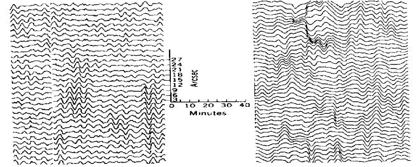
Figure 1: Observations of Doppler velocities on the solar disk, when carried out in one spatial dimension and time, reveal the 5-min oscillations as apparent wave packets that last for about five or six wave periods (Musman and Rust 1970). Right figure illustrates the spatial intensity variations with time (Nishikawa et.al 1986).

Oscillations of the sun’s photosphere were first discovered in the early 1960s (Leighton 1960; Leighton et. al. 1962). Doppler shifts of the spectral lines formed in the atmosphere revealed the period of oscillations of about five minutes. Later it was discovered (Deubner 1975) from theoretical investigations (Ulrich 1970; Leibacher and Stein 1971) that these oscillations are due to superposition of large number of individual modes each having its own characteristics frequency. Surface observations indicate the velocity fluctuations are $\sim$ 1000 m/sec. Where as amplitude of individual modes ranges from 0.3 m/sec to 0.01 m/sec (Fig 1). Some of the groups (Severney et. al. 1976; Kotov et. al. 1978; Scherrer et.al. 1979; Scherrer and Wilcox 1983) reported the oscillations that may represent internal gravity modes. Observations of whole disc Doppler velocities revealed an oscillation with a period 160.01 minute that is believed to be a g mode oscillation of the sun. Thus new era in the history of solar physics viz., seismology of the sun or helioseismology (as this term is initially coined by Severny et. al. 1979) has started that is yielding rich dividends on physics of the sun’s interior.

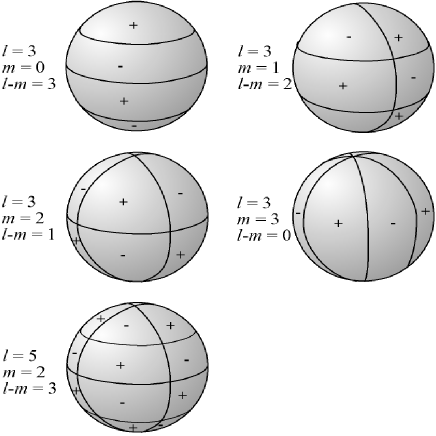
Figure 2: Schematic representation of $Y_{l,m}$ on the unit sphere and its nodal lines. $Y_{l,m}$ is equal to $0$ along $m$ great circles passing through the poles, and along $l-m$ circles of equal latitude. The function changes sign each time it crosses one of these lines. This figure is adopted from Wikipedia.

3.1 Surface Patterns of the Global Oscillation Modes

In spherical coordinates, one can express velocity $V$ of oscillation in a specific normal mode as the real part of

$$V(r,\vartheta,\phi,t)=V_{n}(r)Y_{l}^{m}(\vartheta,\phi)e^{-2\pi\nu t}\,,$$ (1)

where $Y_{l}^{m}(\vartheta,\phi)=P_{l}^{m}(cos\vartheta)e^{im\phi}$ is spherical harmonic function of degree $l$ and azimuthal order $m$, $\vartheta$ is co-latitude and $\phi$ is longitude of the sun.

For each pair of $l$ and $m$, there is a discrete spectrum of modes with distinct frequency $\nu$. These differ in spatial structures as a function of radius. $V_{n}(r)$ are the eigen functions which are oscillatory in space and typically possess $n$ zeros or nodes in the radial direction. The degree $l$ can be understood as the number of complete circles on the surface of a star where the normal component of velocity is always zero.

The angular degree $l$ is related to the total horizontal component of the wave number, $K_{h}$ as

$$K_{h}=\frac{[l(l+1)]^{1/2}}{R_{\odot}}\,,$$ (2)

where $R_{\odot}$ is the radius of the star. Thus high degree $l$ modes sense the near surface structure and very low degree $l$ modes sense near center of the sun. Thus with different degree modes observed on the surface, one can infer the internal structure of sun. The azimuthal order m, characterizes the orientation of the mode relative to the axis of the spherical coordinate system and has $(2l+1)$ values (i.e., $-l,....,l)$. The zero velocity lines are like lines of latitude when $m=0$ and are like lines of longitude when $m=\pm l$. When $m=0$, the spherical harmonic is called as zonal harmonics and the harmonic with $m=l$ is called sectoral harmonics. Tesseral harmonics is obtained when $m\neq l$ (see Fig 2).

3.2 Amplitudes, Frequencies and Line widths of 5 min Oscillations

There are two ways, viz., unimaged and imaged methods, of measuring the amplitudes and frequencies of 5 min oscillations (Hill, Deubner and Isaak 1991). In case of unimaged method, oscillations are due to low-$l$ modes that are obtained from the integrated whole disk measurements. These modes have longer life times ($\sim$ of months) and hence their frequencies can be accurately measured.

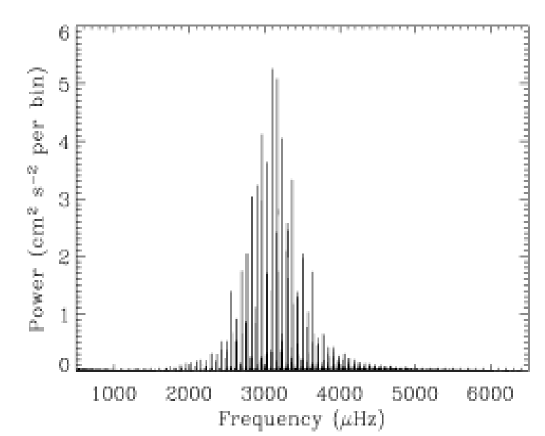
Figure 3: Power spectrum of integrated low degree $p$ modes (Deubner and Gough 1984).

Fig 3 illustrates an example of low-$l$ power spectrum obtained from Birmingham integrated whole disk measurements. One can notice from Fig 3 that, significant power lies between the 1-5 mHz. From the spherical Fourier analysis, it is concluded that these observed oscillations are identified as low degree ($l=0,1,2$ and $3$) and low radial order ($0\leq n\leq 10$) acoustic modes that penetrate deeply the solar interior.

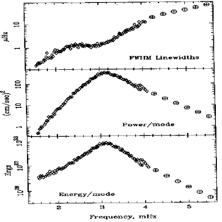
Figure 4: Line width (top), power per mode (middle) and total energy per mode (bottom) as a function of frequency $p$ modes for the modes $l=20$ are illustrated (Libbrecht 1988).

As for the measured amplitudes of oscillations in Doppler velocity, it depends upon the choice of the spectral lines (that occur at different heights ) used for sensing the oscillations. For example, in potassium and sodium lines, maximum amplitudes from the power spectra are estimated to be $\sim$ 15 and 25 $cm^{-1}$ respectively. In case of irradiance, amplitude of oscillations is estimated to be $\sim$ 2-3 x $10^{-6}$. One can get the tables of amplitudes of oscillations from the observations of Doppler velocity measurements (Grec et. al. 1983; Palle et.al. 1989; and Anguera Guba et. al. 1990).

In case of imaged method, amplitudes and frequencies of the solar oscillations are computed from the spatially resolved disk of the sun. With this method, amplitudes and frequencies of many individual modes can be computed. For example, from the information of measured amplitudes, one can get the information of power and energy per mode. For the degree $l=20$, power and energy per mode of oscillations as a function of frequency are illustrated in Fig 4.

Another useful physical parameter measured from the nonimaged and imaged observations is the line width of different oscillation modes that provide vital information of excitation and damping mechanism of the solar oscillations. Measurements of line widths suggests that line width increases with both the frequency ($\nu$) and degree ($l$) of the oscillations. For example, for $l=20$, in Fig 4, FWHM (Full width at half maximum) of the line widths as a function of frequency is illustrated. When one compares the observations of line width as a function of frequency and theoretical estimates (Goldreich and Kumar 1988; Kumar et. al. 1988; Kumar and Goldreich 1989; Dalsgaard et. al. 1989), it is found that growth of the individual modes probably is constrained by the perturbations of the oscillations rather than non-linear interaction among the individual modes.

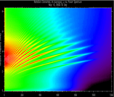
Figure 5: Typical $l$-$\nu$ diagnostic diagram of the $p$ modes: (i) on the left from one day of GONG observations (image courtesy NSO/GONG, Howe) and, on the right side one day Hinode observations (image courtesy Hinode/SOT, Sekii).

3.3 Observed l-$\nu$ν Diagnostic Power Spectrum of the Oscillations

For the imaged observations, continuous and long series of oscillation data set is subjected to spherical harmonic Fourier analysis, averaged over different $m$ azimuthal modes that ensures the removal of effect of sun’s rotation and l-$\nu$ diagnostic ν power spectrum of the solar oscillations is obtained. In Fig 5, such a l-$\nu$νdiagnostic power spectrum is illustrated. In this figure, one can notice that maximum power is concentrated near a frequency of 3 mHz that corresponds to a period of 5 minutes. Another notable interesting characteristic property of this l-$\nu$ν diagnostic diagram is that concentration of power is not distributed randomly, rather it is systematically concentrated in the narrow curved ridges indicating that observed oscillations are due to internal standing waves (confined within the resonant cavity) whose amplitudes vary from central core to near the surface.

3.4 Frequency Splittings due to Rotation and Magnetic Field

In the previous section, solar power spectrum is presented by removing the effect of rotation. Presence of rotation, Coriolis force and magnetic field of the sun affect on the dynamics of the oscillations and hence on the frequencies. For example, if the sun is not rotating, non-magnetic and spherically symmetric, then the modes with same $n$ and $l$, oscillation frequencies would be degenerate in azimuthal order $m$. However, sun is rotating and magnetic resulting in lifting the degeneracy that makes the frequencies depend upon the azimuthal order $m$. In case of sun, compared to magnitudes of rotation and magnetic field structures, effects due to Coriolis and centrifugal forces are negligible. From the observed data, rotational frequency splittings are computed as $\delta\nu_{nlm}=\nu_{nlm}-\bar{\nu}_{nl}$, where $\bar{\nu}_{nl}$ is average frequency for $m=0$. In Fig 6, typical power spectrum of solar oscillations, for different $m$ with $l=20$, obtained from the Big Bear Solar Observatory (Libbrecht 1989) is presented. Clearly one can notice the frequency splittings due to rotation in this illustration.

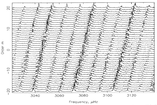
Figure 6: For l=20 and different m, observed frequency splittings due to rotation of the sun (Libbrecht 1989).

Traditionally frequency splittings are related to frequency $\nu_{nlm}$ of a mode as follows

$$\nu_{nlm}=\nu_{nl}+\sum_{i=1}^{i_{max}}a_{i}(nl)P_{i}^{nl}(m)\,,$$ (3)

where $a_{i}$ are the splitting coefficients and $P$ are the polynomials related to Clebsch-Gordon coefficients. Odd degree splitting coefficients $a$ are due to rotational effects and the combined effects (of perturbations due to magnetic field structure, structural asphericities and second order effect due to rotation) contribute to the even degree splitting coefficients.

4 Helioseismic Inferences of Thermal, Dynamic and Magnetic field Structures

Since the discovery of sunspots by Galileo, scientists’ quest is to understand the physics of the sun’s interior. From the helioseismic observations, one can precisely estimate the frequencies and their splittings of different modes of oscillations. For example, by knowing difference between computed theoretical and observationally estimated frequencies, one can infer thermal structure such as internal sound speed and density of the solar interior. Where as the frequency splittings are used for the inference of internal dynamics (such as steady and time dependent parts of rotation and angular momentum ) and magnetic field structures respectively.

4.1 Inference of Thermal Structure by Comparing the Observed and Computed Frequencies

Thermal structure of the solar interior can be understood in the following two ways. By using information of macro and micro physics of the solar interior, compute theoretical frequencies (Dalsgaard 2003; Unno et. al 1989) and match with the observed frequencies. Macrophysics involves standard hydrodynamic equations that are to be linearized and the perturbed variables are assumed to vary with $e^{i\omega t}$, where $\omega$ is angular frequency. Where as micro physics requires other additional details of the solar interior, viz., equation of state, opacity and rate of nuclear energy generation. Using macro and micro physics, with additional knowledge of physics of the convection, solar internal structure such as pressure, temperature, density, etc., are computed.

As the observed amplitudes of oscillations are very small, equation of energy can be neglected and, linearized adiabatic equations with appropriate boundary conditions are used to compute the theoretical frequencies and are matched (Dalsgaard 2003; Unno et. al 1989) with the observed frequencies. Although most of the observed frequencies perfectly match very well for the low and intermediate degree modes, computed frequencies do not match very well with the high degree modes. Possibly this suggests our poor knowledge of physics of near surface effects.

4.1.1 Inference of Thermal Structure: Primary Inversions

In another method, observed frequencies and model of the solar structure are used to invert the thermal structure (for example, sound speed and density) of the solar interior in the following way. For the case of adiabatic oscillations, with additional constraint of conservation of mass, generalized form of equation (Lynden-Bell and Ostriker 1967; Gough and Taylor 1984; Unno et. al. 1989; Dalsgaard 2003) of oscillation that takes into account the effects of velocity flows $\vec{v}$ and magnetic field structure $\vec{B}$ is given as follows

$$\mathcal{L}(\vec{\xi})-\rho\omega^{2}\vec{\xi}+\nabla\delta p+\rho[\omega\mathcal{M}(\vec{\xi})+\mathcal{N}(\vec{\xi})+\mathcal{B}(\vec{\xi})]=0\,,$$ (4)

where

$$\mathcal{L}(\vec{\xi})=\nabla(c^{2}\rho\nabla.\vec{\xi}+\nabla P.\vec{\xi})-g\nabla.(\rho\vec{\xi})-G\rho\nabla(\int_{V}{\nabla.(\rho\vec{\xi})dV\over|\vec{r}-\vec{r}^{{}^{\prime}}|})\,,$$ (5)

$$\mathcal{M}(\vec{\xi})=2i[\vec{\Omega}_{0}\times\vec{\xi}+(\vec{v}\cdot\nabla)\vec{\xi}]\,,$$ (6)

$$\mathcal{N}(\vec{\xi})=(\vec{v}\cdot\nabla)^{2}\vec{\xi}-2\vec{\Omega}_{0}\times[(\vec{\xi}\cdot\nabla)\vec{v}-(\vec{v}\cdot\nabla)\vec{\xi}]-(\vec{\xi}\cdot\nabla)(\vec{v}\cdot\nabla)\vec{v}\,,$$ (7)

$$\mathcal{B}(\vec{\xi})=(4\pi\rho)^{-1}\big{[}[\rho^{-1}(\vec{\xi}\cdot\nabla)\rho+\nabla\cdot\vec{\xi}]\vec{B}\times(\nabla\times\vec{B})-[(\nabla\times\vec{B}^{{}^{\prime}})\times\vec{B}+[(\nabla\times\vec{B})\times\vec{B}^{{}^{\prime}}]\big{]}\,,$$ (8)

where $\mathcal{L}$ is differential operator, $\vec{\xi}$ is eigen function of oscillations, $c$ is speed of sound, $\rho$ is density, $P$ is pressure, $\mathcal{M}(\vec{\xi})$ and $\mathcal{N}(\vec{\xi})$ are effects due to velocity flows, $\mathcal{B}(\vec{\xi})$ is effect due to magnetic field structure and other symbols have usual meanings. Although effects due to flows and magnetic field structure in the solar interior can not be neglected, for simplicity, these terms are neglected and with special boundary conditions such that density and pressure perturbations completely vanish at the surface, equation (4) leads to the form $\mathcal{L}(\vec{\xi})=\rho\omega^{2}\vec{\xi}$. This equation is an eigen value problem and is also Hermitian. Hence, variational principle (Chandrasekhar 1964; see also Unno et. al. 1989) can be used to linearize the equation and frequency difference $\delta\nu_{n,l}$ between the sun and standard solar structure model can be represented (Basu 2010 and references there in) as follows

$${\delta\nu_{n,l}\over\nu_{n,l}}=\int_{0}^{R}K_{c^{2},\rho}^{nl}(r){\delta c^{2}\over c^{2}}(r)dr+\int_{0}^{R}K_{\rho,c^{2}}^{nl}(r){\delta\rho\over\rho}(r)dr+{F(\nu_{n,l})\over E_{nl}}\,,$$ (9)

where $K_{c^{2},\rho}^{nl}(r)$ and $K_{\rho,c^{2}}^{nl}(r)$ are kernels that involve eigen functions of the oscillations and the known solar structure. Other terms $\delta c^{2}\over c^{2}$ and $\delta\rho\over\rho$ are the differences of sound speed and density between the sun and the reference solar structure model. The last term (see for details Basu 2010) is a correction due to surface effects and does not arise due to linearization. Hence, from the observed oscillation frequencies and with the known reference solar structure model, one can invert radial profiles of $\delta c^{2}\over c^{2}$ and $\delta\rho\over\rho$ in the solar interior. There are many inversion techniques (Gough and Thompson 1991; Unno et. al. 1989; Dalsgaard 2002 and references there in) to infer these profiles and one such inversion that yields the differences of sound speed and density (between the sun and the solar structure model) is presented (Basu et. al. 2009) in Fig 7.

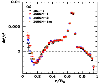
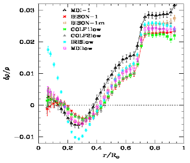
Figure 7: Inference of thermal structure: (i) Left figure illustrates the sound speed difference between the sun and the model and, (ii) right figure illustrates the density difference between the sun and the model. Image courtesy, Basu.

It is interesting to note that most of the models (Basu 2010 and references there in) almost match with the reference solar structure models, yet there are unexplained statistically significant sound speed differences mainly near base of the convection zone and in the radiative core. Similarly, density profile of solar structure models developed so far do not match very well with the density profile of the real sun. All of the solar structure models require the surface chemical heavy elemental abundances $Z$ (or ratio $Z/X$, where $X$ is the hydrogen abundance) that indirectly contribute to the equation of state and the opacity and hence, ultimately affect the computed frequencies, modeled sound speed and density structures. Most of these models (Basu 2010 and references there in) used the heavy elemental abundance ratio ($Z/X$=0.0229) by Grevesse and Noels (1993). However, recent determination (Asplund et.al. 2000, 2004; Allende Prieto et.al 2001, 2002) lowered this ratio ($Z/X$ = 0.0166) leading to further deterioration of match between sound speed of the sun and different models. Hence, this conundrum of unexplained differences of thermal structures of sound speed and density is remained to be explained.

4.1.2 Inference of Thermal Structure: Secondary Inversions

By knowing the reference solar structure model, in the previous section, observed frequencies are used to compute the thermal structure differences of sound speed and the density. From these differences and knowing the sound speed and density structures as determined by the reference models, one can obtain sound speed and density profiles of the sun. As the sound speed and the density structures are thermodynamic quantities, in the following, using stellar structure equations (with additional information of equation of state and the opacity structures), one can uniquely obtain the thermal structure of the solar interior. There are two advantages of this solar seismic model, as in the standard solar models, (i) no assumption of history of the sun and, (ii) no need to have adhock computation of the convective flux. In addition, chemical compositions such as hydrogen and helium abundances are obtained as part of solution. Thus, in essence, this seismic model yields a snap shot model of the present day sun.

For example, if equation of state of the solar plasma is available, inverted sound speed can be constrained to yield the ratio $T/\mu$ (where $T$ is temperature and $\mu$ is the mean atomic weight). Following are the four set of stellar structure differential equations that need to be solved by imposing sound speed obtained by the primary inversions

$${dM_{r}\over dr}=4\pi r^{2}\rho\,,$$ (10)

$${dP\over dr}=-{GM_{r}\rho\over r^{2}}\,,$$ (11)

$${dL_{r}\over dr}=4\pi r^{2}\rho\epsilon\,,$$ (12)

$${dT\over dr}=-\frac{3}{4ac}\frac{\kappa\rho}{T^{3}}\frac{L_{r}}{4\pi r^{2}}\,\,\,\,\,\,\,\,if\,\,radiative\,,$$

$$=({dT\over dr})_{conv}\,\,\,\,\,\,if\,\,convective\,,$$ (13)

where the radial variables $M_{r}$, $P$, $L_{r}$ and $T$ are the mass, pressure, luminosity and temperature respectively. Other variables $\epsilon$, $\kappa$ and $({dT\over dr})_{conv}$ are the rate of nuclear energy generation, opacity of matter and knowledge of convective energy transport in the outer 30 $\%$ of the sun. Further axillary equations such as equation of state, equations of opacity and rate of nuclear energy generation are required. It is assumed that sun is in mechanical and thermal equilibrium such that whatever energy generated in the deep radiative core must be transported to the surface. However this latter condition can not be guaranteed.

As the sound speed is thermodynamically determined quantity, it is a function of other three variables, viz., pressure, temperature and the chemical composition. As for the chemical composition, hydrogen $X$ and helium $Y$ are separately considered and all other elements are treated as single entity and is called as heavy elemental abundance $Z$.

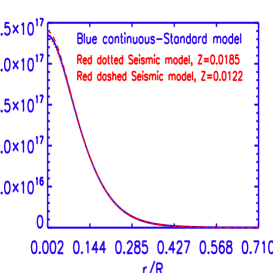
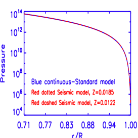
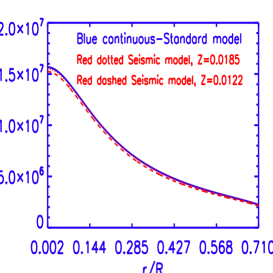
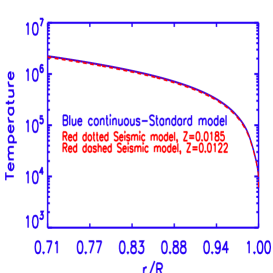
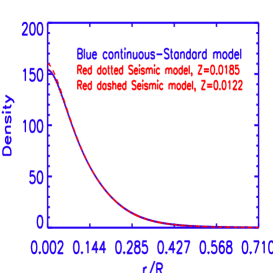
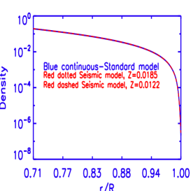
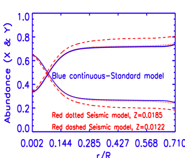
Figure 8: Thermal structure such as pressure, temperature, density and hydrogen abundance $X$ and helium abundance $Y$ obtained by the solar seismic model for surface heavy elemental abundances $Z=0.0185$ and $Z=0.0122$ respectively. Units are in cgs scale.

With appropriate boundary conditions and assuming $Z$ as constant, earlier models (Shibahashi, Takata and Tanuma 1994; Shibahashi and Takata 1996; Shibahashi and Takata 1997; Takata and Shibahashi 1998; Antia and Chitre 1999) solved above equations by considering the radiative core only. Although deduced profiles of thermal structure are almost similar to the profiles of solar standard models, there is no guarantee that these deductions satisfy the observed luminosity and the mass. By considering the inverted sound speed (Takata and Shibahashi 1998) for the whole region from center to the surface, a global seismic model (Shibahashi, Hiremath and Takata 1998a; Shibahashi, Hiremath and Takata 1998b; Shibahashi, Hiremath and Takata 1999) is developed that satisfies both the observed luminosity and the mass. It is found that seismic model satisfying one solar mass at the surface varies strongly on the nature of the sound speed profile near the center and a weak function of either depth of the convection zone or heavy elemental abundance Z/X. It is also found that one solar mass at the surface is satisfied for the sound speed profile which deviates at the center by $\sim$ 0.22% from the sound speed profile of solar model (Cristensen Dalsgaard 1996), if we adopt the value of nuclear cross section factor $S_{11}$ value of 4.07 $\times 10^{-22}$ keV barns. The resulting chemical abundances at base of the convective envelope are obtained to be $X=0.755$, $Y=0.226$ and $Z=0.0185$ in case computed chemical abundance ratio $Z/X=0.0245$ matches with the earlier (Grevesse and Noels 1993) chemical abundance ratio. Neutrino fluxes of different reactions are computed and are not different than the neutrino fluxes computed from the standard solar model.

Table 1. Neutrino Fluxes (in the units of $10^{10}cm^{-2}sec^{-1}$)
estimated by the solar seismic model.
$Source$	SSM	Seism1	Seism2	Seism3	Seism4
	Z=0.0185	Z=0.0185	Z=0.0165	Z=0.015	Z=0.0122
	Z/X=0.0247	Z/X=0.0247	Z/X=0.0215	Z/X=0.0188	Z/X=0.0158
	BCZ=0.709	BCZ=0.709	BCZ=0.709	BCZ=0.709	BCZ=0.72
pp	6.0	6.01	6.05	6.07	6.1
pep	0.014	0.015	0.014	0.015	0.015
hep	8$\times 10^{-7}$	0.3$\times 10^{-9}$	0.3$\times 10^{-9}$	1.3$\times 10^{-7}$	1.32$\times 10^{-7}$
7Be	0.47	0.44	0.42	0.41	0.379
8B	5.8$\times 10^{-4}$	4.5$\times 10^{-4}$	4.03$\times 10^{-4}$	3.76$\times 10^{-4}$	3.18$\times 10^{-4}$
13N	0.06	0.057	0.047	0.04	0.0287
${}^{15}O$	0.05	0.052	0.042	0.036	0.025
${}^{17}F$	$5.2\times 10^{-4}$	$4.02\times 10^{-4}$	3.2$\times 10^{-4}$	2.7$\times 10^{-4}$	1.92$\times 10^{-4}$

Recently, by considering the inverted sound speed kindly provided by Antia, thermal structure and neutrino fluxes are computed. One can notice from the Fig 8 that the deduced internal structural parameters such as mass, luminosity, pressure, density and temperature are almost similar to the structural parameters obtained by the standard solar models. Neutrino fluxes computed by using sound speed profile computed from the standard model and the seismic models with different $Z$ values are presented in Table 1. In Table 1, nomenclatures for SSM, Seism and BCZ are standard solar model of Dalsgaard (1996), seismic model and base of the convection zone respectively.

One can notice that, for the earlier (Grevesse and Noels 1993) chemical abundance ratio $Z/X=0.0247$, neutrino fluxes (Table 1) computed from the seismic model is not different from the neutrino fluxes computed from the solar standard solar model that lead to a turning point with a strong conclusion that deficiency of neutrinos emitted by the sun lies in the neutrino physics ruling out the astrophysical solutions. Even changing of uncertain physics of the interior, such as opacity, equation of state, etc., or chemical composition (especially the heavy elemental abundance $Z$) could not alleviate the solar neutrino problem.

However and surprisingly, for the recently determined heavy elemental abundance ($Z/X=0.016$; seismic model 4, Table 1), neutrino flux, especially for ⁸B is substantially reduced and is almost similar to the observed neutrino fluxes, although helium abundance deduced by this seismic model at the base of the convective envelope is very low ($\sim$ 0.18) and is inconsistent with other cosmic helium abundances ($\sim$ 0.23). Recent determination (Asplund 2004) of heavy elemental abundances (that substantially lowered the abundances of carbon, nitrogen, oxygen and neon) has given a rebirth of astrophysical solution to the solar neutrino problem (Turck-Chièze et.al. 2010; Turck-Chièze and Couvidat 2011).

4.2 Inference of Dynamic Structure

The term dynamic structure is mainly due to rotation of the whole sun, although large-scale weak meridional flow ($\sim$ few meters/sec from equator to both the northern and southern poles) and strong convective flows in the interior exist. Observations show that, with a typical linear velocity of $\sim$ 2 km/sec, sun rotates differentially, rotating faster at the equator and slower at the poles. As mentioned in section 3.4, rotation of the sun lifts the degeneracy of the oscillations that leads to frequency of oscillations depend upon azimuthal order $m$ and, similar to Zeeman effect, split the frequencies yielding a relation $\omega_{m}=\omega_{0}+\Omega m$ (where $\omega_{0}$ is frequency of the oscillations in the rotating frame of reference and $\Omega$ is the angular velocity of the sun). In this simple description, angular velocity $\Omega$ is assumed to be of rigid body rotation and hence is independent of radius and latitude respectively. Observations show that sun is rotating differentially and, by neglecting the effects due to centrifugal force and the magnetic field structure, equation (4) can be modified (Unno et.al. 1989; Dalsgaard 2002; Dalsgaard 2003; Thompson et.al. 2003) as follows

$$\delta\omega_{nlm}=\omega_{nlm}-\omega_{nl0}=m\int_{0}^{R}\int_{0}^{\pi}K_{nlm}(r,\theta)\Omega(r,\theta)rdrd\theta\,,$$ (14)

where the kernels (Hansen et. al. 1977; Cuypers 1980; Schou et. al. 1994) $K_{nlm}(r,\theta)$ involve the eigen functions of oscillations in the nonrotating frame. These kernels depend only upon $m^{2}$ and hence the rotational splittings ($\omega_{nlm}-\omega_{nl0}$) are odd function of $m$. As the kernels are also symmetrical about the equator, the rotational splittings sense only the symmetrical component of $\Omega$. From the observed rotational splittings and the computed kernels $K_{nlm}(r,\theta)$ from the adiabatic oscillations, one can invert the equation (14) and hence rotation rate $\Omega(r,\theta)$ of the whole region of the solar interior is obtained. There are different inversional techniques (Dalsgaard and Schou 1988; Schou et. al. 1994; Pijpers and Thompson 1992, 1994; Sekii 1996; Kosovichev et. al. 1996; Korzennik et.al. 1996; Antia, Basu and Chitre 1998; Thompson et. al. 2003 and references therein; Howe 2009 and references there in; Antia and Basu 2010) and inferred rotation rate of the solar interior is presented in Fig 9.

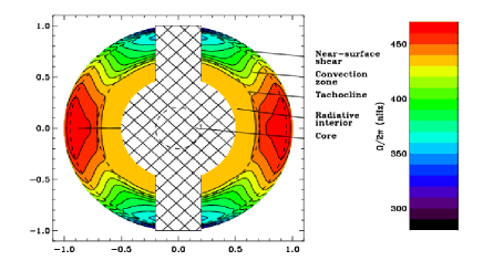
Figure 9: Isorotational contours inferred from 12 years average data of MDI data. The cross hatched areas indicate the regions in which it is difficult or impossible to obtain reliable inversion results with the available data (Courtesy : Howe).

One can notice from Fig 9 that sun rotates differentially in the entire convective envelope and has a rigid body rotation rate in the radiative core. In addition, near the surface and the base of convection zone, two rotational shears exist. The rotational shear near base of convection zone, where the transition from differential rotation to rigid body rotation occurs, is called tachocline where the seat of so called dynamo (that is believed to be origin and maintenance of solar cycle and activity phenomena) is supposed to exist (Hiremath 2010; Hiremath and Lovely 2012 and references there in). However, yet it is not completely understood how the sun attained such a rotational structure in its interior.

4.3 Inference of Magnetic Field Structure

Recent observations suggest that the entire universe is pervaded by a large scale weak uniform magnetic field structure (Ryu et.al. 2011 and references there in) and sun is also no exception. The sun is pervaded by a large scale steady (diffusion time scale of $\sim$ billion yrs) global dipole like magnetic field structure with a strength of $\sim$ 1 G (Stenflo 1993) and time dependent magnetic field structure ($\sim$ kilo gauss) that fluctuates over 22 years. If magnetic field lines vary from pole to pole, such a geometry is called poloidal field structure. Where as in case of toroidal field structure, field lines are parallel to the equator. Sun is pervaded by a combined weak ($\sim$ 1 G) poloidal and strong ($\sim$ $10^{3}$ G) toroidal field structure. Sunspots are supposed to be formed due to Alfven perturbations of the steady toroidal magnetic field structure (Hiremath and Lovely 2012) embedded in the solar interior. Large scale magnetic field structure induces a force and distorts the geometrical figure of a star. During the early evolutionary history of the sun, magnetic field structure might have played a dominant role in transferring angular momentum to the solar system. This could be one of the main reasons why most of the angular momentum is concentrated in the solar system rather than in the sun. It is believed that 22 yr magnetic cycle is due to so called dynamo mechanism that is the result of interplay of convection and rotation on the large scale poloidal magnetic field structure although there are other alternative views (Hiremath 2010; Hiremath and Lovely 2012).

4.3.1 Inference of Magnetic Field Structure : Primary Inversions

Signatures of both the poloidal and toroidal magnetic field structures can be found in the observed even degree frequency splittings. In addition, second order rotational effect (where as first order or linear rotational effect is sensed by the odd degree frequency splittings as given in section 4.2) and aspherical sound speed perturbations (Kuhn 1988) also contribute to the even degree frequency splittings. Hence, by assuming that aspherical sound speed perturbations are negligible, with the internal rotational structure as inferred from the helioseismology (section 4.2), contribution due to second order rotational effects is computed and is subtracted from the even degree frequency splittings and, resulting residual of even degree splittings are compared with the computed frequency splittings due to assumed magnetic field structure. Detailed inversion procedures can be found in the previous studies (Dziembowski and Goode 1989; Gough and Thompson 1991; Dziembowski and Goode 1991; Basu 1997; Antia, Chitre and Thompson 2000; Antia 2002; Baldner et. al. 2010). Recently Baldner et. al. (2010) came to the conclusion that the observed variation of even degree frequency splittings can be explained if the sun is pervaded by a right combination of poloidal ($\sim$ 100 G) and toroidal (that varies from $\sim$ $10^{3}$ G near the surface to $10^{4}$ G near base of the convection zone) magnetic field structure. By considering the SOHO/MDI magnetograms and from the analysis of sunspot data during their initial appearance on the surface, recently, Hiremath and Lovely (2012) estimated strength of toroidal magnetic field structure of similar order confirming the previous theoretical estimates (Choudhuri and Gilman 1987; D’Silva and Choudhuri 1993; D’Silva and Howard 1994; Hiremath 2001).

4.3.2 Inversion of Poloidal Magnetic Field Structure : Secondary Inversions

Owing to large diffusion time scales due to large dimension and finite conductivity of the solar plasma, sun might have retained a large scale poloidal magnetic structure from its protostar phase even after the convective Hayashi phase (Cowling 1953; Layzer, Rosner and Doyle 1979; Piddington 1983; Mestel and Weiss 1987; Spruit 1990). Presence of such a large scale poloidal magnetic field structure, especially during the solar minimum, can be clearly discerned during the solar total eclipse. Field lines of dipole like magnetic field structure are clearly delineated in the intensity patterns of the white light pictures taken during the eclipse. If the Lorentz force due to either poloidal or toroidal magnetic field structure is very weak compared to dynamical effects such as rotation, one can show (Hiremath 1994; Hiremath and Gokhale 1995) that weak poloidal magnetic field structure isorotates with the solar plasma. In fact, in case of the sun, especially for the poloidal magnetic field structure ($\sim$ 1 G), this condition is valid. That means, if $\Omega$ is angular velocity of the plasma and $\Phi$ is the magnetic flux function representing flux of the poloidal magnetic field structure, one can show that

$$\Omega=function(\Phi)\,.$$ (15)

If one knows the internal rotational structure of the sun, by suitable combination of poloidal magnetic field structure that is obtained consistently from the solution of MHD equations, one can satisfy the above condition. To a first approximation, right hand side of equation can be linearized of the form

$$\Omega=\Omega_{0}+\Omega_{1}(\Phi)\,.$$ (16)

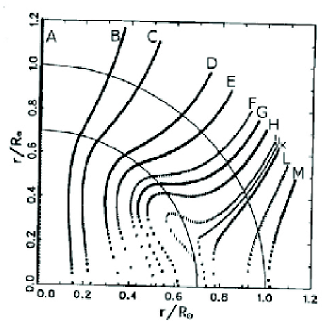
Figure 10: Left figure illustrates the meridional cross section of poloidal component of magnetic field structure. This figure is reproduced from, and all rights are reserved by, the Astrophysical Journal. Where as right figure illustrates radial and latitudinal variations of the magnitude of the poloidal magnetic field structure $B_{p}$ normalized to an asymptotic uniform magnetic field that merges with the interplanetary field structure.

With reasonable assumptions and approximations and by using Chandrasekhar’s (1956a; 1956b) MHD equations for the case of axisymmetry and incompressibility, Hiremath and Gokhale (1995) have shown that poloidal component of the sun’s steady magnetic field structure can be modeled as an analytical solution of magnetic diffusion equation and the magnetic flux function $(\Phi)$ for both the radiative core (RC) and the convective envelope (CE) are expressed as

$$\Phi_{RC}(x,\vartheta)=2\pi A_{0}R_{c}^{2}x^{1/2}sin^{2}\vartheta\sum_{n=0}^{\infty}\lambda_{n}J_{n+3/2}(\alpha_{n}x)C_{n}^{3/2}(\mu)\,,$$ (17)

where $x=r/R_{c}$, $R_{c}$ is radius of the radiative core, $\mu=cos\vartheta$, $r$ and $\vartheta$ are radial and colatitude coordinates, $n$ is non negative integer, $C_{n}^{3/2}$ is the Gegenbaur’s polynomial of degree $n$, $J_{n+3/2}(\alpha_{n}x)$ is Bessel function of order $(n+3/2)$ and $\alpha_{n}$ are the eigen values that are to be determined from the boundary conditions. Here $A_{0}$ is taken as a scale factor for the field and hence $\lambda_{n}=A_{n}/A_{0}$. Similarly, magnetic flux function for the case of convective envelope is

$$\Phi_{CE}(x,\vartheta)=\pi B_{0}R_{c}^{2}sin^{2}\vartheta\big{[}x^{2}C_{0}^{3/2}(\mu)+\sum_{n\geq 0}\hat{\mu}_{n+1}x^{-(n+1)}C_{n}^{3/2}(\mu)\big{]}\,,$$ (18)

where $\hat{\mu}_{n+1}=M_{n}/(\pi B_{0}R_{c}^{n+3})$ are strengths of multipoles that are scaled to an asymptotically uniform magnetic field structure $B_{0}$. One can notice from the above equation that magnetic field structure approaches an asymptotically uniform field structure as $x\rightarrow\infty$. With appropriate boundary conditions at base of the convection zone and with helioseismically inferred rotation, one can uniquely estimate the unknown coefficients and eigen values respectively. In case of sun and with the available helioseismically inferred rotation (Dziembowski et. al. 1989; Antia, Basu and Chitre 1998), geometry of the poloidal field structure is computed (Hiremath 1994; Hiremath and Gokhale 1995) and is presented in Fig 10. If one considers strength of interplanetary magnetic field structure ($\sim 10^{-5}$ G) as a scaling factor, strength of sun’s poloidal magnetic field structure near its center is found to be $\sim 10^{7}-10^{8}$ G. From the dynamical constraints, one can rule out such a strong magnetic field structure near the center. However, if the 22 yr solar cycle and activity phenomenon is due to global slow MHD modes (Hiremath and Gokhale 1995), $B_{0}$ is estimated to be $\sim 10^{-2}$ G and, in that case strength of poloidal magnetic field structure near the center turns out be $\sim 10^{5}$ G. Off course one would have found signature of such a strong field structure in the observations of $p$ mode oscillations. Unfortunately low degree ‘p’ modes that penetrate deeply in the radiative core can not sense close to the center. Hence, one has to wait for the discovery of elusive $g$ modes that are highly sensitive to the central structure of the sun and hence their characteristics are modified (Rashba 2006, 2007, 2008; Burgess et. al. 2004) by such a strong magnetic field structure.

5 Concluding Remarks

Although seismology of the sun has provided some of the detailed global aspects of thermal and dynamic structures of the sun’s interior, other global structures such as detailed informations regarding meridional flow (this information is needed to accept or reject so called flux transport dynamo models) and magnetic field structure are necessary. Hitherto solar seismologists came to the conclusion that the difference between the sun’s thermal structure (especially the sound speed) and the modeled thermal structure is almost similar. However, recent revision of heavy-element abundances (Asplund et. ali. 2000, 2004; Allende Prieto et.al. 2001, 2002; Asplund et. ali. 2005) that are reduced drastically, further worsened the difference between the sun’s and modeled thermal structure leading to revisit of exotic astrophysical solutions that are used to explain the solar neutrino problem. Importantly, as noticed by the previous studies (Chaplin and Basu 2008; Basu and Antia 2008), critical examination of modeling and method of computation in estimating the heavy-elemental abundance are necessary.

As for the dynamical helioseismic inferences, especially the rotational structure, ‘p’ modes are not the true representatives to sense the deep radiative core. For this purpose one has to wait for discovery of ‘g’ modes that have high sensitivity near the core. Hence knowing of magnitude and form (i.e., dependent or independent of radius and latitude) of thermal and rotational structures near the core are essential for understanding overall structure and temporal variations of the sun on short ($\sim$ 11 years) and long ($\sim$ billion years) time scales. Although helioseismic inferences of rotation rate of the convective envelope ruled out the increase of rotation rate (as is assumed to be in the earlier turbulent dynamo models) from surface to the interior and cylindrical isorotational contours (simulations by Gilman and Miller 1981), physics of isorotational contours, especially near the surface, is completely not understood. However, it should be appreciated that the simulated isorotational contours from base of convection zone to $0.935R_{\odot}$ (Kitchatinov and Rudiger 1995; Elliot et. al 2000; Robinson and Chan 2001, Hiremath 2001; Brun and Toomre 2002, Rempel 2005; Meisch et. al. 2006; Kuker, Rudiger and Kitchatinov 2011; Brun et.al 2011) are almost similar to the rotational isocontours as inferred from helioseismology although none of the present simulations reproduce the near surface decreasing rotational profile from $0.935R_{\odot}$ to the surface. Even if numerical simulations achieve the goal of reproducing near surface rotational profile, from the MHD stability criterion (Dubrulle and Knobloch 1993; Mestel 1999), $r^{2}{d\over dr}[{\Omega^{2}\over r^{2}}]-({1\over r^{2}}){d\over dr}[{(r^{2}B_{\phi}^{2})\over 4\pi\rho}]>0$ (where $r$ is the radial coordinate, $\Omega$ is angular velocity, $\rho$ is density and $B_{\phi}$ is toroidal magnetic field structure), one can show that such a decreasing rotational profile near the surface is unstable (independently, Miesch and Hindman 2011, recently came to a similar conclusion) unless sun acquired near equipartition toroidal magnetic field structure. Interestingly, toroidal field structure estimated by theoretical (Hiremath 2001; Brun, Miesch and Toomre 2004) and helioseismic (Antia 2002; Baldner et.al. 2010) inferences yield of similar magnitudes. Hence, near surface rotational profile is stable.

However, why the sun acquired such a decreasing near surface rotational profile and hence the toroidal magnetic field structure are remained to be explained. Although beyond the scope of this presentation, such a near surface decreasing rotational profile can be explained if one speculates that during the early history of the planetary formation, protoplanetary mass that rotated with Keplerian velocity might have accreted on to the sun that resulted in winding of threaded ambient large scale poloidal magnetic field structure into toroidal magnetic field structure. If this speculation is correct, such a protoplanetary accretion scenario might give some clues regarding absence of super earths near vicinity of the sun and peculiar high solar mass (Gustafsson 2008) compared to other stars in the sun’s neighborhood in the Galaxy. Incase we accept the accretion scenario (during the early solar system formation), longstanding problems such as angular momentum and planetary formation of the solar system can be solved. With such an accretion scenario and hence high solar mass, unsolved faint young sun paradox (Minton and Malhotra 2007) and recent puzzle of computation of low heavy elemental abundances (Asplund et. al. 2005) that are incompatible (Basu et al. 2007; Basu and Antia 2008) with the helioseismic inferences can also be alleviated upto some extent (Winnick et. al. 2002; Haxton and Serenelli 2008; Nordlund 2009; Meléndez et. al. 2009; Guzik and Mussack 2010 and references there in; Serenelli et.al. 2011).

As for the secondary inversion of poloidal magnetic field structure, this method requires the rotational profile of the interior as inferred by the helioseismology for estimation of different magnetic moments. Instead, as the weak ($\sim$ 1 G) poloidal magnetic field structure isorotates with the internal rotation of the plasma and hence rotation is a function of magnetic flux, equation (14) can be used for simultaneously inverting rotational and poloidal magnetic field structures of the interior (Gokhale and Cristensen Dalsgaard, private communication).

References

Agnihotri, R., Dutta, K and Soon, W. 2011, JASTP, 73, 1980

Anguera Gubau, M., Palle, P. L., Hernandez, P and Roca-Cortes, T. 1990, Sol Phys, 128, 79

Antia, H. M., Basu, Sarbani & Chitre, S. M. 1998, MNRAS, 298, 543

Antia, H. M and Chitre, S. M. 1999, A&A, 347, 1000

Antia, H. M., Chitre, S. M., & Thompson, M. J. 2000, A&A, 360, 335

Antia, H. M. 2002, Proceedings of IAU Coll. 188, ESA SP-505, p.71

Antia, H. M. & Basu, S., 2010, ApJ, 720, 494

Allende Prieto, C., Lambert, D.L., Asplund, M. 2001. ApJ. 556, L63

Allende Prieto, C., Lambert, D.L., Asplund, M. 2002. ApJ. 573, L137

Asplund, M., Nordlund, Trampedach, R., Stein, R.F. 2000, A & A, 359, 743

Asplund, M., Grevesse, N., Sauval, A.J., Allende Prieto, C., Kiselman, D. 2004, Astron. Astrophys. 417, 751

Asplund, M., Grevesse, N and Sauval, A. J. 2005, ASP Conf. Series 336, p. 25

Baldner, C. S., Antia, H. M; Basu, S and Larson, T. P. 2010, Astronomische Nachrichten, 331, 879

Basu, S. 1997, MNRAS, 288, 572

Basu, S., Chaplin, W. J., Elsworth, Y., New, R., Serenelli, A. M., & Verner, G. A. 2007, ApJ, 655, 660

Basu, S and Antia, H. M. 2008, Physics Reports, 457, 217

Basu, S., Chaplin, W. J., Elsworth, Y, New, R and Serenelli, A. M. 2009, ApJ, 699, 1403

Basu, S. 2010, Astrophys & Space Sci, 328, 43

Brun, A. S., Miesch, M. S and Toomre, J. 2004, ApJ, 614, 1073

Brun, A. S. & Toomre, J. 2002, ApJ, 570, 865

Brun, A. S., Miesch, M. S., & Toomre, J. 2011, ApJ, 742, 79

Burgess, C. P., Dzhalilov, N. S., Rashba, T. I., Semikoz, V. B and Valle, J. W. F., 2004, MNRAS, 348, 609

Chandrasekhar, S. 1956a, ApJ, 124, 232

Chandrasekhar, S. 1956b, ApJ, 124, 244

Chandrasekhar, S. 1964, ApJ, 139, 664

Chaplin, W. J and Basu, S, 2008, Sol Phys, 251, 53

Choudhuri, A. R and Gilman, P. A. 1987, ApJ, 316, 788

Cowling, T. G. 1953, MNRAS, 94, 39

Cuypers, J. 1980, A&A, 89, 207

Dalsgaard, C., Gough, D. O and and Libbrecht, K. B. ApJ, 341, L103

Dalsgaard, C., et al. 1996, Science, 272, 1286

Dalsgaard, C. 2003, Lecture Notes on Stellar Oscillations, p. 66

Dalsgaard, C. 2002, Rev. Mod. Phys. 74, 1073

Deubner, F.-L. 1975, A&A, 44, 371

Deubner, F.-L and Gough, D. 1984, ARA & A, 22, 593

D’Silva, S., & Choudhuri, A. R. 1993, A&A, 272, 621

D’Silva, S., & Howard, R. 1994, Sol Phys, 151, 213

Dubrulle, B & Knobloch, E., 1993, A&A, 274, 667

Dziembowski, W. A and Goode, P. R. 1989, ApJ, 347, 540

Dziembowski, W. A., Goode, P. R and Libbrecht, K. G. 1989, ApJ, 343, L53

Dziembowski, W. A and Goode, P. R. 1991, ApJ, 376, 782

Elliott, J. R., Miesch, M. S., & Toomre, J. 2000, ApJ, 533, 546

Feynman, J. 2007, AdSpR, 40. 1173

Gilman, P. A and Miller, J. 1981, ApJS, 46, 211

Goldreich, P and Kumar, P. 1988, ApJ, 326, 462

Gough, D. O and Taylor, P. P. 1984, Mem. Soc. Astron. Ital., 55, 215

Gough, D. O and Thompson, M. J. 1991, in Solar Interior and Atmosphere, . p. 519

Grec, G., Fossat, E and Pomerantz, M. 1983, Sol Phys, 82

Grevesse, S and Noels, A. 1993, : in Origin and Evolution of the Elements, p. 15

Guzik, J. A and Mussack, K., 2010, ApJ, 713, 1108

Haigh, J. D. 2007, Living Rev Sol Phys, 4, 2

Hansen, C. J., Cox, J. P and Van Horn, H. M. 1977, ApJ, 217, 151

Haxton, W. C. and Serenelli, A. M. 2008, ApJ, 687, 678

Hill, G., Deubner, F. L and Isaak, G. 1991, in Solar Interior and Atmosphere, p. 329

Hiremath, K. M. 1994, PhD Thesis, Bangalore University

Hiremath, K. M and Gokhale, M. H. 1995, ApJ, 448, 437

Hiremath, K. M. 2001, Bull Astron Soc India, 29, 169

Hiremath, K. M and Mandi, P. I. 2004, NewA, 9, 651

Hiremath, K. M. 2006a, Journal of Astrophysics and Astronomy, vol 27, 367

Hiremath, K. M. 2006b, Journal of Astrophysics and Astronomy, vol 27, 277

Hiremath, K. M. 2006c, in the proceedings of ILWS workshop, Goa, p. 178

Hiremath, K. M. 2008, Ap & SS, 314, 45

Hiremath, K. M. 2009, Sun & Geosphere, 4, 16

Hiremath, K. M. 2010, Sun & Geosphere, 5, 17

Hiremath, K. M and Lovely, M. R. 2012, New Astronomy, 17, 392

Howe, R. 2009, Living Review in Solar Phys, 6, 1

Kitchatinov, L. L. and Rüdiger, G. 1995, A&A, 299, 446

Kuhn, J. R. 1988, ApJ, 331, L131

Kuker, M., Rudiger, G and Kitchatinov, L. L. 2011, A&A, 530, 48

Kumar, P., Franklin, J and Goldreich, P. 1988, ApJ, 328, 879

Kumar, P and Goldreich, P. 1989, ApJ, 343, 558

Korzennik, S. G., Thompson, M. J and Toomre, J. 1996, in IAU Symp 181, p. 211

Kotov, V. A., Severnyi, A. B and Tsap, T. T. 1978, MNRAS, 183, 61

Layzer, D., Rosner, R and Doyle, H. T. 1979, ApJ, 229, 1126

Leibacher, J. W and Stein, R. F. 1971, ApJL, 7, 191L

Leighton, R. B. 1960, IAUS, 12, 321

Leighton, R. B., Noyes, Robert W and Simon, George W. 1962, ApJ, 135, 474

Libbrecht, K. G. 1988, ApJ, 334, 510

Libbrecht, K. G. 1989, ApJ, 336, 1092

Lynden-Bell, D and Ostriker, J. P. 1967, MNRAS, 136, 293

Miesch, M. S., Brun, A. S and Toomre, J. 2006, ApJ, 641, 618

Miesch, M. S and Hindman, B. W. 2011, ApJ, 743, 79

Minton, D. A and Malhotra, R., 2007, ApJ, 660, 1700

Meléndez, J., Asplund, M., Gustafsson, B and Yong, D. 2009, ApJ, 704, L66

Mestel, L and Weiss, N. O. 1987, MNRAS, 226, 123

Musman, S and Rust, D. M. 1970, Solar Phys, 13, 261

Nishikawa, J., Hamana, S., Mizugaki, K and Hirayama, T. 1986, Publ. Astron. Soc. Japan, 38, 277

Nordlund, A. 2009, arXiv:0908.3479

Palle, P. L., Regulo, C and Roca-Cortes, T. 1989, A & A, 224, 253

Perry, C, A. 2007, AdSpR, 40, 353

Piddington, J. H. 1983, Astrophys Space Sci, 90, 217

Pijpers, F. P and Thompson, M. J. 1992, A&A, 262, 33

Pijpers, F. P and Thompson, M. J. 1994, A&A, 281, 231

Rashba, T. I., Semikoz, V. B and Valle, J. W. F., MNRAS, 370, 845, 2006

Rashba, T. 2008, Journ Physics: Conf Ser, 118, p. 012085

Rashba, T. I., Semikoz, V. B., Turck-Chièze, S and Valle, J. W. F. 2007, MNRAS, 377, 453

Reid, G. C. 1999, JASTP, 61, 3

Rempel, M. 2005, ApJ, 622, 1320

Robinson, F. J and Chan, K. L. 2001, MNRAS, 321, 723

Ryu, D., Schleicher, D. R. G. Treumann, R. A., Tsagas, C. G., Widrow, L. M. 2011, Space Science Reviews, 312

Scafetta, N and West, B. J., 2008, Physics Today, March Issue, p. 50-51

Scherrer, P. H., Wilcox, J. M., Kotov, V. A., Severny, A. B and Tsap, T. T. 1979 Nature, 277, 635

Scherrer, P. H and Wilcox, J. M. 1983, Sol Phy, 82, 37

Schou, J., Christensen-Dalsgaard, J and Thompson, M. J. 1994, ApJ, 433, 389

Serenelli, A. M., Haxton, W. C & Pena-Garay, C., 2011, arXiv:1104.1639

Sekii, T. 1996, in IAU Symp 181, p. 189

Severnyi, A. B., Kotov, V. A., Tsap, T. T. 1976, Nature, 259, 87

Severnyi, A. B., Kotov, V. A and Tsap, T. T. 1979, Soviet Astronomy, 23 641

Shibahashi, H., Takata, M and Tanuma, S. 1995, ESA SP, Proceedings of the 4th Soho Workshop, p. 9

Shibahashi, H and Takata, M. 1996, PASJ, 48, 377

Shibahashi, H and Takata, M. 1997, 1997, IAU Symp 181, 167

Shibahashi, H., Hiremath, K. M and Takata, M. 1998a, ESASP, 418, 537

Shibahashi, H., Hiremath, K. M and Takata, M. 1998b, IAU Symp, 185, 81

Shibahashi, H., Hiremath, K. M and Takata, M. 1999, Advance Space Res, 24, 177

Shine, K, P. 2000, SSRv, 94, 363

Soon, W. 2005, Geophys. Res. Let, 32, 16, L16712

Spruit, H. C. 1990, in Inside the Sun, p. 415

Stenflo, J. O. 1993, in Solar Surface Magnetism

Takata, M and Shibahashi, H. 1998, ApJ, 504, 1035

Thompson, Michael J., Christensen-Dalsgaard, Jørgen, Miesch, Mark S. & Toomre, J. 2003, Astron Astrophys Rev, 41, 599

Tiwari, M and Ramesh, R. 2007, Current Science, vol 93, 477

Turck-Chièze, S., Palacios, A., Marques, J. P and Nghiem, P. A. P. 2010, ApJ, 715, 1539

Turck-Chièze, S and Couvidat, S. 2011, Rep Prog Phys, 74, 086901

Ulrich, Roger K. 1970, ApJ, 162, 99

Unno, W., Osaki, Y., Ando, H., Sao, H and Shibahashi, H. 1989, in ”Noradial Oscillations of Stars”, p. 108

Winnick, R. A., Demarque, P., Basu, S., & Guenther, D. B. 2002, ApJ, 576, 1075