Density functional approaches to collective phenomena in nuclei: Time-dependent density-functional theory for perturbative and non-perturbative nuclear dynamics

Abstract

We present the basic concepts and our recent developments in the density functional approaches with the Skyrme functionals for describing nuclear dynamics at low energy. The time-dependent density-functional theory (TDDFT) is utilized for the exact linear response with an external perturbation. For description of collective dynamics beyond the perturbative regime, we present a theory of a decoupled collective submanifold to describe for a slow motion based on the TDDFT. Selected applications are shown to demonstrate the quality of their performance and feasibility. Advantages and disadvantages in the numerical aspects are also discussed.

1 Introduction

1.1 Nucleus as a quantum object

The nuclei provide the matters with mass, the stars with fuel, and the universe with a variety of elements. It was discovered by Ernest Rutherford and coworkers about 100 years ago Rut1911 , that explains the large-angle scattering of alpha particles by a gold foil GM1909 . This discovery was also a beginning of the era of the quantum mechanics. Rutherford estimated the upper limit of the nuclear size which turned out to be much smaller than that of the atom. In the atomic scale (Å), the nuclear size (fm) could be regarded as just a point! According to the classical mechanics, the atoms must collapse into nuclear size, because the attractive Coulomb potential eventually brings all the electrons into the nucleus. This mystery stimulated Niels Bohr to develop his idea on the quantum mechanics Bohr1913 .

1.1.1 Atoms and molecules

With a knowledge of the quantum mechanics, it is easy to understand why the atoms do not collapse to the nuclear scale. If an electron was confined in the nuclear scale of femtometer, the uncertainty principle immediately tells us that its zero-point kinetic energy would become gigantic (order of GeV). In order to decrease this kinetic energy to a reasonable magnitude, the electron’s wave function must have an atomic size of Å. Thus, the atomic size is a consequence of the quantum effect.

The molecules (and the solids) are a good contrast to atoms. The atom is bound by the Coulomb interaction, whose range is infinite ($V_{N-e}\sim-Ze^{2}/r$), between a positively charged nucleus and electrons with a negative charge. Since the molecules consist of these charge-neutral atoms, the interaction between a pair of neutral atoms does not have the long-range tail of $1/r$, but normally has a short-range repulsive part and an intermediate-range attractive part (Fig. 1(a)). Because of this charge neutrality, the molecule is easy to disintegrate into smaller units (molecules and atoms). The atomic size is approximately constant and independent from the atomic number, while the molecular size varies depending on the number of atoms and their kinds. Last but not the least, in the zero-th order approximation, the ground states of the molecules can be classically described as atoms located at fixed relative positions. The hindered quantum fluctuation in molecules is simply due to the fact that the atomic mass, which is approximately identical to the nuclear mass, is about 2,000 times larger than the electronic mass.

1.1.2 Nuclei

The nucleus has a number of properties analogous to the molecules, except for its strong quantum nature. It is a self-bound system composed of fermions of spin $1/2$ and isospin $1/2$ with approximately equal masses, called nucleons (protons and neutrons). The nuclear species are classified by the numbers of neutrons ($N$) and protons ($Z$). Rutherford discovered that the size of the nucleus is as tiny as the femtometer, but later it was found that the nuclear size varies, as its volume is roughly proportional to the mass number ($A=N+Z$). Each nucleon is a color-singlet (neutral) object. The interaction between a pair of nucleons (nuclear force) has a finite range of a scale of the pion Compton wave length ($\lambda_{\pi}$). Similar to the molecules, it has a short-range repulsive part and an intermediate-range attractive part (Fig. 1(b)). The nucleus can be disintegrated into small pieces with a small separation energy. In fact, heavy nuclei can have “negative” separation energies because of the repulsive Coulomb energy among protons.

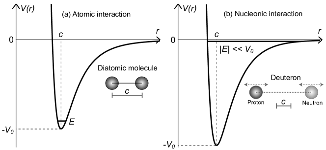
Figure 1: Schematic representation of atomic and nucleonic interactions $V(r)$ as a function of the relative distance $r$. The energy of the bound (ground) state $E$ is shown by a horizontal line. (a) Atom-atom interaction: $V_{0}=1\sim 10$ eV and $c\approx a_{B}$, where $a_{B}$ is the Bohr radius. (b) Nucleon-nucleon interaction: $V_{0}\approx 100$ MeV and $c=0.5\sim 1$ fm. The essence of the present figure is taken from Fig. 2-36 in Ref. BM69 .

The quantum nature is an important difference between the nucleus and the molecule. In Fig. 1, we show schematic pictures of the atomic and nucleonic potentials. The ground state of the diatomic molecule (panel (a)) is formed at the bottom of the potential, $E\approx-V_{0}$. In the length scale of Å, the atomic mass is heavy enough to localize the wave function at the location of the bottom of the potential, $r\approx c$. Thus, the relative distance between a pair of atoms is fixed at $r=c$. This property allows us to describe the atomic motion in the classical mechanics, such as in the molecular dynamics. In contrast, the nuclear interaction is not strong enough to bind nucleons at the bottom of the potential. In other words, the nucleon’s mass is too light to localize the wave function in the sub-femtometer scale. In deuteron, the zero-point kinetic energy cancels the negative potential energy ($\langle T+V\rangle\approx 0$), leading to a bound state at approximately zero energy ($E=-2.2\mbox{ MeV}\gg-V_{0}$). The deuteron wave function spatially extends beyond the range of nuclear force ($\sim\lambda_{\pi}$), which reduces the kinetic energy $\langle T\rangle$. This shows a striking contrast to the diatomic molecule, and is even analogous to the atoms, that the large size of the deuteron is a consequence of the quantum effect. This strong quantum nature also tells us that the infinite nuclear matter will not be crystallized even at zero temperature, but will stay as the liquid. The nuclear system provides us with unique opportunities to study femto-scale quantum liquids.

1.2 Computing nucleus from scratch

The strong quantum nature in finite nuclei leads to a rich variety of unique phenomena. Remarkable experimental progress in production and study of exotic nuclei requires us to construct theoretical and computational approaches with high accuracy and a reliable predictive power. Extensive studies have been made for constructing theoretical models to elucidate basic nuclear dynamics behind a variety of nuclear phenomena. Simultaneously, significant efforts have been made in the microscopic foundation of those models.

For light nuclei, the “first-principles” large-scale computation, starting from the bare nucleon-nucleon (two-body & three-body) forces, is becoming a current trend in theoretical nuclear physics. Among them, the Green’s function Monte Carlo (GFMC) method is the most successful first-principles approach to nuclear structure calculation PW01 . In this approach, using the Monte Carlo technique, the many-body wave function is sampled in the coordinate space with spin and isospin degrees of freedom. The success of the GFMC clearly demonstrates that we are able to construct a light nucleus from the scratch on the computer. The GFMC method has been applied to nuclei up to the mass number $A\approx 10$. Another first-principles approach is to project the nuclear Hamiltonian in a truncated Hilbert space, then diagonalize it. This is called no-core shell-model (NCSM) method NNBV06 . The NCSM also shows successful applications up to the $p$-shell nuclei. The GFMC and NCSM both indicate the exponential increase in computational tasks with respect to the increasing nucleon number. The third approach, the coupled-cluster method (CCM), has an advantage that the required computation increases only in power with respect to the nucleon number. The CCM, which was originally invented in nuclear physics KLZ78 and later became extremely successful in quantum chemistry BM07 , has been revisited as an ab-initio computational approach to nuclear structure Wlo05 . Especially, it is powerful to study closed-shell nuclei.

Although these first-principles approaches have recently shown a significant progress, they are still limited to nuclei with the small mass number. This may sound mysterious to physicists in other fields, because we know that the similar kinds of approaches are able to treat systems of much larger particle numbers. For instance, using the CCM, nowadays, the chemists can easily calculate a molecular structure with 100 electrons. Why is the first-principles calculation of nuclear structure so difficult? The answer is perhaps trivial for nuclear physicists, but may not be so for others. Let us pick up several important aspects leading to this answer. (1) The strong quantum nature. As we have discussed previously, the full quantum mechanical treatment is necessary for nuclear structure calculation. (2) Strong coupling nature. The nucleon-nucleon scattering length is approximately $a\approx-18$ fm in ${}^{1}S_{0}$ channel. This is much larger than the mean distance between nucleons inside the nucleus ($k_{F}|a|\gg 1$). (3) Singular property of the nucleonic interaction. To reproduce the phase shift for the nucleon-nucleon scattering, the interaction should have a strong repulsive core at short distance BM69 . (4) Complexity of the nucleonic interaction. The interaction has a strong state dependence which may be represented by the spin- and isospin-dependence BM69 . It also contains strong non-central and non-local terms, such as tensor and spin-orbit interactions. Furthermore, for a quantitative description of nuclei, it is indispensable to introduce three-body interactions in addition to the two-body force. (5) Coexistence of different interactions. In addition to the strong interaction, we need to treat the electromagnetic interactions among protons. (6) Coexistence of different energy scales. The nuclear binding energy amounts to order of GeV for heavy nuclei. Because of the strong quantum nature in nuclei, this is a consequence of the cancellation between positive kinetic energy and negative potential energy. Thus, we need to compute these enormous positive and negative components in high accuracy to obtain a correct binding energy. (7) Fermionic nature of nucleons. Needless to say, since the nucleons are fermions, the total wave function must be anti-symmetrized. (8) Finite systems without an external potential. Electronic many-body problems in molecules and solids are solved with external fields produced by nuclei with positive charges. In contrast, the nucleus is a self-bound finite system. Thus, we are usually required to obtain an intrinsic wave function without the center-of-mass degrees of freedom. This requirement often restricts our choice of the basis functions.

Despite of these difficulties, significant advances in the computer power may lead to a realistic “first-principles” construction of the $sd$-shell nuclei in near future. There have been extensive efforts toward this direction, especially developing an algorithm suitable for parallel use of the vast number of processors unedf .

1.3 Density functional theory (DFT)

In contrast to the first-principles calculations, which are limited to nuclei with small number of nucleons, the density functional theory (DFT) is currently a leading theory for describing nuclear properties of heavy nuclei BHR03 ; LPT03 . It is capable of describing almost all nuclei, including nuclear matter, with a single universal energy density functional (EDF). An argument based on the quantum many-body theory leading to nuclear EDF was also developed in 70’s$-$80’s Neg82 ; Nak11 . In addition, its strict theoretical foundation is given by the basic theorem of the DFT HK64 ; KS65 . Since the nucleus is a self-bound system without an external potential, we should slightly modify the DFT theorem. This will be discussed in Sec. 2.

The nucleus by itself produces a potential confining nucleons which is analogous to the Kohn-Sham potential in DFT KS65 . Nuclear physicists often call this potential “mean field”, though it is different from a naive mean-field potential directly constructed from the nucleonic interaction. There are many evidences for the fact that the mean-free path of nucleons inside the nucleus is significantly larger than the nuclear radius BM69 , in spite of the strong (and even singular) two-body interaction. This is partially due to the Pauli exclusion principle. Since the nucleon mean-free path is roughly proportional to $\left\{\epsilon_{F}/(\epsilon-\epsilon_{F})\right\}^{2}$ Gal58 , it is significantly enhanced for nucleons whose energies are close to the Fermi energy. Another even simpler argument was given by Bohr and Mottelson BM69 , that the nuclear normal density is much lower than the one giving the close packing limit (crystalline limit). In this argument, the quantum effect plays a primary role.

The DFT theorem guarantees the existence of generalized density functionals for every physical observable (see Sec. 2). However, to construct the exact functional, we need experimental data and other theoretical inputs. Currently, there are a variety of EDFs which predict somewhat different properties for nuclei very far from the stability line. We are in want of finding an ultimate universal energy density functional, which is capable of exact description of every nucleus in the nuclear chart. In addition to the recent progress in the first-principles calculations for light nuclei, the radioactive beam facilities in the world will give us ideal opportunities to determine the parameter set for a better functional. New data on neutron halos and skins in medium heavy nuclei may provide important information on its dependence on density and density gradient. Observation of new isotopes in a long isotopic (isotonic) chain may lead to useful constraints on the isovector parts of the energy functional.

An extension of the DFT to the time-dependent DFT (TDDFT) provides a feasible description of many-body dynamics, which contains information on excited states in addition to the ground state. The TDDFT is justified by the one-to-one correspondence between the time-dependent density and time-dependent external potential RG84 , which will be presented in Sec. 2.4. The TDDFT has vast applications to quantum phenomena in many-body systems. Among them, the perturbative regime has been mostly studied so far. Different approaches to the linear response calculations will be presented in Sec. 3. It is of significant interest but challenging to go beyond the perturbative regime. Nuclei show numerous phenomena related to the large amplitude collective motion, such as fission, shape transition, shape coexistence, anharmonic vibrations, and so on. We present, in Sec. 4, a theory to identify an optimal collective submanifold in the classical phase space of large dimensions.

2 Basic formalism for particles in self-bound systems

The density functional theory (DFT) has been extremely successful for calculations of ground-state properties of atoms, molecules, and solids. It describes a many-particle system exactly in terms of its one-body density alone. The DFT is based on the original theorem of Hohenberg and Kohn (HK) HK64 which was proved for the ground-state of the many-particle system. Every observable can be written, in principle, as a functional of density.

In nuclear physics, however, we need to treat an isolated system without an external potential. The present nuclear EDF produces a localized density profile without an external potential. Thus, the ground state spontaneously violates the translational symmetry and seems to contain spurious excitation related to the center-of-mass motion. Furthermore, it also violates the rotational symmetry when the ground state is spontaneously deformed. It is interesting to see whether the nuclear EDF can be theoretically justified in a strict sense. We present a possible justification in Sec. 2.1, according to the recent progress Eng07 ; Gir08 ; GJB08 .

2.1 DFT theorem for a wave-packet state

The HK theorem HK64 guarantees one-to-one mapping between a one-body density $\rho(\vec{r})$ and an external potential $v_{0}(\vec{r})$. Then, since the ground-state wave function is a functional of density, in principle, all the observables should be functionals of the density as well. However, to describe an isolated self-bound finite system in a box of volume $V$, it is somewhat useless to use the ground-state density in the laboratory frame, because it must be constant, $\rho(\vec{r})=\rho=N/V\rightarrow 0$ ($V\rightarrow\infty$), where $N$ is the particle number. Instead, we want to use a functional of the intrinsic density $\rho(\vec{r}-\vec{R})$, where $\vec{R}$ is the center-of-mass coordinate of the total system. In this case, the original HK theorem cannot be justified, because it adopts a one-body external field $v_{0}(\vec{r})$ coupled to the density $\rho(\vec{r})$ in the laboratory frame.

Validity of the DFT for the intrinsic states has been discussed by several authors Eng07 ; Gir08 ; GJB08 . In this section, we present a method to define the DFT for an intrinsic state, more precisely for a “wave-packet” state. The argument here essentially follows the idea by Giraud et al GJB08 .

In fact, all the nuclear EDFs, currently available, produce a wave-packet state. The minimization of an EDF $E[\rho]$ without the external potential ($v_{0}(\vec{r})\rightarrow 0$) leads to the nucleon density distribution $\rho(\vec{r})$ with a finite radius. This violates the translational symmetry of the original Hamiltonian. Therefore, it is of our interest here to justify the energy functional of the wave-packet density in the laboratory frame in a strict sense.

First, we assume that a wave-packet state in the laboratory frame can be expressed by a product wave function of intrinsic and spurious degrees of freedom, $|{\Phi}\rangle=|{\phi}\rangle\otimes|{\chi}\rangle$. Here, $|{\phi}\rangle$ indicates the intrinsic state and $|{\chi}\rangle$ defines the spurious motion. This decomposition can be exactly done for the translational motion.

$$H=H_{\rm intr}(\xi,\pi)+\frac{\vec{P}^{2}}{2Nm},$$ (1)

$$\Phi(\vec{r}_{1},\cdots,\vec{r}_{N})=\phi(\vec{\xi}_{1},\cdots,\vec{\xi}_{N-1})\otimes\chi(\vec{R}),$$ (2)

where $\vec{R}$ $(\vec{P})$ denote the center-of-mass coordinates (total momenta). $\vec{\xi}_{i}$ and $\vec{\pi}_{i}$ are the relative Jacobi coordinates and their conjugate momenta, respectively. Since the intrinsic ground state, which is supposed to be unique, is completely independent from the spurious motion, we can adopt an arbitrary form of $\chi(\vec{R})$; e.g., $\chi(\vec{R})\propto\exp(-R^{2}/2b^{2})$. Then, the ground wave-packet state can be obtained by the variation after the projection:

$$(E_{0})_{\chi}\equiv\min_{\chi{\rm:fixed}}\left[\frac{\langle{\Phi}|HP|{\Phi}\rangle}{\langle{\Phi}|P|{\Phi}\rangle}\right]$$ (3)

where the projection operator $P$ does not change the intrinsic state $|{\phi}\rangle$ but makes $\chi(\vec{R})$ an eigenstate of the total linear momentum $P=0$. The variation with respect to the full space ($|{\Phi}\rangle=|{\phi}\rangle\otimes|{\chi}\rangle$) contradicts the uniqueness of the ground state, because states with different $\chi(\vec{R})$ give the same $P|{\Phi}\rangle$. Therefore, the variation here should be performed with respect only to the intrinsic state $|{\phi}\rangle$. This is indicated by the subscript “$\chi$:fixed” in Eq. (3). The wave-packet density profile is simply given by $\rho(\vec{r})\equiv\langle{\Phi}|\hat{\psi}^{\dagger}(\vec{r})\hat{\psi}(\vec{r})|{\Phi}\rangle$, that depends on the form of $\chi(\vec{R})$. In the followings, we always assume a fixed form of $\chi(\vec{R})$ for the wave-packet state $|{\Phi}\rangle$.

Next, we introduce an external potential $V_{0}=\sum_{i}v_{0}(\vec{r}_{i})$. The following minimization with respect to the intrinsic state $|{\phi}\rangle$ leads to the “minimum” energy $E_{0}[v_{0}]$ and defines the wave packet $|{\Phi}\rangle$.

$$E_{0}[v_{0}]=\min_{\chi{\rm:fixed}}\left[\frac{\langle{\Phi}|HP|{\Phi}\rangle}{\langle{\Phi}|P|{\Phi}\rangle}+\langle{\Phi}|V_{0}|{\Phi}\rangle\right]=\min_{\chi{\rm:fixed}}\left[\frac{\langle{\Phi}|HP|{\Phi}\rangle}{\langle{\Phi}|P|{\Phi}\rangle}+\int\rho(\vec{r})v_{0}(\vec{r})d^{3}r\right].$$ (4)

Noted that $V_{0}$ operates on a state $|{\Phi}\rangle$, not on a projected state $P|{\Phi}\rangle$. $E_{0}[v_{0}]$ does not correspond to the ground-state energy of a system with the Hamiltonian $H+V_{0}$, however, it reduces to Eq. (3) for $V_{0}=0$. Now, let us show the one-to-one correspondence between the external potential $V_{0}$ and the wave-packet density $\rho(\vec{r})$. The proof proceeds by reductio ad absurdum in the same manner as the original proof of HK HK64 . Assume that another potential $v^{\prime}_{0}(\vec{r})$, which defines the wave packet $|{\Phi^{\prime}}\rangle$, produces the same density $\rho(\vec{r})$. Then, the energy for $|{\Phi^{\prime}}\rangle$ is given by

$$E_{0}[v_{0}^{\prime}]=\frac{\langle{\Phi^{\prime}}|HP|{\Phi^{\prime}}\rangle}{\langle{\Phi^{\prime}}|P|{\Phi^{\prime}}\rangle}+\langle{\Phi^{\prime}}|V_{0}^{\prime}|{\Phi^{\prime}}\rangle.$$ (5)

If we replace the state $|{\Phi^{\prime}}\rangle$ by $|{\Phi}\rangle$, the energy must increase.

$$E_{0}[v_{0}^{\prime}] < \frac{\langle{\Phi}|HP|{\Phi}\rangle}{\langle{\Phi}|P|{\Phi}\rangle}+\langle{\Phi}|V_{0}^{\prime}|{\Phi}\rangle$$ (6)

$$= \frac{\langle{\Phi}|HP|{\Phi}\rangle}{\langle{\Phi}|P|{\Phi}\rangle}+\langle{\Phi}|V_{0}|{\Phi}\rangle+\langle{\Phi}|V_{0}^{\prime}-V_{0}|{\Phi}\rangle$$

$$= E_{0}[v_{0}]+\int\rho(\vec{r})\left\{v_{0}^{\prime}(\vec{r})-v_{0}(\vec{r})\right\}d^{3}r.$$

Interchanging $V_{0}$ and $V_{0}^{\prime}$, we also find

$$E_{0}[v_{0}]<E_{0}[v_{0}^{\prime}]+\int\rho(\vec{r})\left\{v_{0}(\vec{r})-v_{0}^{\prime}(\vec{r})\right\}d^{3}r.$$ (7)

Addition of Eqs. (6) and (7) leads to the inconsistency, $E_{0}[v_{0}]+E_{0}[v_{0}^{\prime}]<E_{0}[v_{0}]+E_{0}[v_{0}^{\prime}]$. This proves the one-to-one correspondence between the external field $V_{0}$ and the wave-packet density $\rho(\vec{r})$. Thus, both $v_{0}(\vec{r})$ and the wave packet $|{\Phi}\rangle$ are functionals of the density $\rho(\vec{r})$. In order to lift restriction to $v$-representative densities, we use the constrained search Lev79 in which one considers only states that produce a given density $\rho(\vec{r})$, and define the universal functional

$$F_{\chi}[\rho]\equiv\min_{\Phi\rightarrow\rho}\left[\frac{\langle{\Phi}|HP|{\Phi}\rangle}{\langle{\Phi}|P|{\Phi}\rangle}\right].$$ (8)

Here, the subscript “$\Phi\rightarrow\rho$” indicates the minimization with a constraint on $\rho(\vec{r})$. The density functional $F_{\chi}[\rho]$ contains the energy of the fixed center-of-mass spurious motion, $E_{\chi}$, that is trivially given by $E_{\chi}(N)\equiv\langle{\chi}|\vec{P}^{2}|{\chi}\rangle/(2Nm)$. Therefore, the energy of the ground state with $P=0$ (intrinsic energy) may be obtained by the minimization with a constraint on the total particle number, as

$$E_{\rm intr}(N)\equiv E_{P=0}(N)=\min_{\rho}\left[F_{\chi}[\rho]-\lambda\left(\int\rho(\vec{r})d^{3}r-N\right)\right]-E_{\chi}(N).$$ (9)

Note that, although the wave function $|{\chi}\rangle$ is fixed, $E_{\chi}$ may depend on the total mass of the system (particle number $N$). In principle, the expectation value of any observable $\hat{O}$, which only depends on the intrinsic degrees of freedom, is a functional of $\rho$,

$${\mathcal{O}}[\rho]\equiv\langle{\phi}|\hat{O}|{\phi}\rangle\times\langle\chi|\chi\rangle=\langle{\Phi}|\hat{O}|{\Phi}\rangle,$$ (10)

because the wave-packet state $|{\Phi}\rangle$ is given as a functional of $\rho$. Since the state $|{\chi}\rangle$ is fixed, there is a trivial correspondence between the wave-packet density $\rho(\vec{r})$ and the intrinsic density $\rho(\vec{r}-\vec{R})$. This completes the basic theorem of the DFT for the wave packet.

2.2 The Kohn-Sham (KS) scheme

For a many-body system of fermions, the shell effects play a major role to determine the ground state. In other words, we need a density functional which takes account of the kinetic energy properly. This is known to be difficult in the local density approximation RS80 . At present, a scheme given by Kohn and Sham KS65 only provides a practical solution for this problem. Here, we follow the same argument.

We introduce a reference system which is a “virtual” non-interacting system with an external potential $v_{s}(\vec{r})$. This reference system is supposed to reproduce the same density $\rho(\vec{r})$ of the “physical” interacting wave packet, but does not have to reproduce the center-of-mass wave function $|{\chi}\rangle$. The ground state of the reference system is trivially obtained as a Slater determinant constructed by the solution of

$$\left(-\frac{1}{2m}\nabla^{2}+v_{s}(\vec{r})\right)\phi_{i}(\vec{r})=\epsilon_{i}\phi_{i}(\vec{r}),$$ (11)

adopting the unit $\hbar=1$, and the density is given by $\rho(\vec{r})=\sum_{i=1}^{N}|\phi_{i}(\vec{r})|^{2}$. The kinetic energy is given by

$$T_{s}[\rho]=\sum_{i=1}^{N}\langle{\phi_{i}}|\left(-\frac{1}{2m}\nabla^{2}\right)|{\phi_{i}}\rangle.$$ (12)

The variation of the total energy of the reference system

$$E_{s}[\rho]=T_{s}[\rho]+\int v_{s}(\vec{r})\rho(\vec{r})d^{3}r,$$ (13)

with a constraint on the particle number, $\delta(E_{s}[\rho]-\mu\int\rho(\vec{r})d^{3}r)=0$, leads to the following equation:

$$\mu=\frac{\delta T_{s}[\rho]}{\delta\rho(\vec{r})}+v_{s}(\vec{r}).$$ (14)

Although we did not explicitly construct $T_{s}[\rho]$ as a functional of $\rho(\vec{r})$, the solution of Eq. (14) must be identical to the solution of Eqs. (11) and (12).

The success of the Kohn-Sham (KS) scheme comes from a simple idea to decompose the kinetic energy in the physical interacting system into two parts; $T_{s}[\rho]$, which is a major origin of the shell effects, and the rest, which is treated as a part of “correlation energy” described by a simple functional of density,

$$F_{\chi}[\rho]=T_{s}[\rho]+E_{c}[\rho],$$ (15)

where $E_{c}[\rho]\equiv F_{\chi}[\rho]-T_{s}[\rho]$. Then, the variation of $F_{\chi}[\rho]$ leads to Eq. (14) but the potential is now a functional of density, defined by $v_{s}(\vec{r})\equiv\delta E_{c}[\rho]/\delta\rho(\vec{r})$. The only practical difference between the reference system and the interacting system is that, since $v_{s}(\vec{r})$ is a functional of density in the latter, Eq. (11) must be self-consistently solved. These equations are called Kohn-Sham (KS) equations. The self-consistent solution of the KS equations provides the density $\rho(\vec{r})$ of a wave-packet state with a fixed $|{\chi}\rangle$ corresponding to a (local) minimum of the EDF, $F_{\chi}[\rho]$. The success of the KS scheme is attributed to the goodness of the local density approximation for $E_{c}[\rho]$.

2.3 Open issues

2.3.1 Subtraction of the center-of-mass energy

In the proof of the basic theorem for the wave packet, given in Sec. 2.1, we need to fix a wave function of the center-of-mass motion $|{\chi}\rangle$. The choice of this spurious wave function is arbitrary, but the energy $E_{\chi}$ depends on this choice. In practice, the subtraction of $E_{\chi}$ is normally performed by constructing the state $|{\chi}\rangle$ from the obtained result. This is somewhat inconsistent with the assumption of the fixed center-of-mass state $|{\chi}\rangle$. This could be easily corrected by taking $E_{\chi}$ of a given $|{\chi}\rangle$. However, as far as we know, this has not been examined yet.

2.3.2 Validity of the Kohn-Sham scheme

The KS scheme is to take into account a major part of the kinetic energy as $T_{s}[\rho]$, and the rest as a correction. In other words, the KS scheme implicitly assumes that the energy $E_{c}[\rho]$ is able to be well approximated by a simple functional of $\rho$. In fact, this question is still an open issue, not only in the nuclear physics but also in other quantum many-body systems. In the present wave-packet theory, the kinetic energy of the wave packet, $T_{\chi}[\rho]=\langle{\Phi}|\hat{T}|{\Phi}\rangle$, depends on the center-of-mass state $\chi(\vec{R})$. Therefore, there may be an optimal choice for $\chi(\vec{R})$ to minimize the difference $T_{\chi}[\rho]-T_{s}[\rho]$. The question about the validity of the Kohn-Sham scheme remains to be answered.

2.3.3 Non-spherical wave packet

The nuclear EDFs are known to produce a spontaneous symmetry breaking about the rotational symmetry. Namely, we often encounter a deformed wave-packet density, which accounts for appearance of the rotational spectra in nuclei. For instance, many experimental evidences indicate that nuclei in the rare-earth region and in the actinide region are deformed BM75 . According to the argument in Sec. 2.1, we may separate the rotational motion from the intrinsic degrees of freedom, then, we have

$$\Phi(\vec{r}_{1},\cdots,\vec{r}_{N})\approx\phi(\xi)\otimes\chi(\vec{\Theta},\vec{R}),$$ (16)

where $\vec{\Theta}$ indicates angle variables. Then, replacing the operator $P$ by that of angular momentum projection, the DFT for deformed wave packet can be shown in the same manner. However, in contrast to the translational motion, the separation of the rotation degrees of freedom is not exact. but only approximate. Thus, there remains an ambiguity for the definition of the functional (8): Namely, the minimization must be performed in the entire space except for the subspace that accounts for translational and rotational correlations. In this sense, the use of the EDF, which produces a deformed state, can be justified only approximately.

2.4 Time-dependent density functional theory

The DFT is designed for calculating the ground-state properties. For excited-state properties and reactions, the time-dependent density functional theory (TDDFT) is a powerful and useful tool. In this section, we recapitulate the basic theorem for the time-dependent density functional theory (TDDFT).

Since the proof of the HK theorem is based on the Rayleigh-Ritz variational principle, its extension to the time-dependent density is not straightforward. This was done by Runge and Gross RG84 , showing that there is one-to-one correspondence between a time-dependent density $\rho(\vec{r},t)$ and a time-dependent external potential $v(\vec{r},t)$. The external potential is required to be expandable in a Taylor series about the initial time $t_{0}$,

$$v(\vec{r},t)=\sum_{k=0}^{\infty}\frac{1}{k!}v_{k}(\vec{r})(t-t_{0})^{k}.$$ (17)

The external potentials, $v(\vec{r},t)$ and $v^{\prime}(\vec{r},t)$, are defined to be different if there exist some minimal nonnegative integer $k$ such that $\nabla w_{k}(\vec{r})\neq 0$ where $w_{k}(\vec{r})\equiv v_{k}(\vec{r})-v^{\prime}_{k}(\vec{r})$. In other words, $v(\vec{r},t)$ and $v^{\prime}(\vec{r},t)$ differ more than a time-dependent function, $v(\vec{r},t)-v^{\prime}(\vec{r},t)\neq c(t)$. Note that the potentials differing by the time-dependent constant $c(t)$ produce the same density $\rho(\vec{r},t)$ because the corresponding wave functions differ by a merely time-dependent phase, as in Eq. (27) with $\alpha(t)=\int^{t}c(s)ds$.

Now, let us assume that starting a common initial state $|{\Psi_{0}}\rangle=|{\Psi(t_{0})}\rangle$, two different external potentials, $v(\vec{r},t)$ and $v^{\prime}(\vec{r},t)$, produce densities $\rho(\vec{r},t)$ and $\rho^{\prime}(\vec{r},t)$, respectively. From this, we first prove that the current densities, $\vec{j}(\vec{r},t)$ and $\vec{j^{\prime}}(\vec{r},t)$, are different. Using the current density operator $\vec{\hat{j}}(\vec{r})$, the equation of motion is written as

$$i\frac{\partial}{\partial t}\vec{j}(\vec{r},t)=\langle{\Psi(t)}|[\vec{\hat{j}}(\vec{r}),\hat{H}(t)]|{\Psi(t)}\rangle,$$ (18)

where $\hat{H}(t)=H_{0}+\sum_{i=1}^{N}v(\vec{r}_{i},t)$. We have the same equation for $\vec{j^{\prime}}(\vec{r},t)$, with $|{\Psi(t)}\rangle$ and $v(\vec{r},t)$ replaced by $|{\Psi^{\prime}(t)}\rangle$ and $v^{\prime}(\vec{r},t)$, respectively. Then, we have

$$\left.\frac{\partial}{\partial t}\left\{\vec{j}(\vec{r},t)-\vec{j^{\prime}}(\vec{r},t)\right\}\right|_{t=t_{0}} = -i\langle{\Psi_{0}}|[\vec{\hat{j}}(\vec{r}),\hat{H}(t_{0})-\hat{H}^{\prime}(t_{0})]|{\Psi_{0}}\rangle$$ (19)

$$= -\frac{1}{m}\rho(\vec{r},t_{0})\nabla w_{0}(\vec{r}).$$

If $\nabla w_{0}(\vec{r})\neq 0$, it is easy to see that $\vec{j}(\vec{r},t)$ and $\vec{j^{\prime}}(\vec{r},t)$ are different at $t>t_{0}$. In case that $\nabla w_{0}(\vec{r})=0$ and $\nabla w_{1}(\vec{r})\neq 0$, we need to further calculate derivative of Eq. (18) with respect to $t$.

$$\left.i\frac{\partial^{2}}{\partial t^{2}}\vec{j}(\vec{r},t)\right|_{t=t_{0}}=\langle{\Psi_{0}}|[\vec{\hat{j}}(\vec{r}),\frac{\partial\hat{H}(t_{0})}{\partial t}]|{\Psi_{0}}\rangle+\langle{\Psi_{0}}|[[\vec{\hat{j}}(\vec{r}),\hat{H}(t_{0})],\hat{H}(t_{0})]|{\Psi_{0}}\rangle.$$ (20)

The second term of Eq. (20) vanishes for $\partial^{2}/\partial t^{2}\{\vec{j}(\vec{r},t)-\vec{j^{\prime}}(\vec{r},t)\}|_{t=t_{0}}$, because $\hat{H}^{\prime}(t_{0})=\hat{H}(t_{0})+\mbox{const}$. Thus,

$$\left.\frac{\partial^{2}}{\partial t^{2}}\left\{\vec{j}(\vec{r},t)-\vec{j^{\prime}}(\vec{r},t)\right\}\right|_{t=t_{0}}=-\frac{1}{m}\rho(\vec{r},t_{0})\nabla w_{1}(\vec{r})\neq 0.$$ (21)

Again, we can conclude that $\vec{j}(\vec{r},t)\neq\vec{j^{\prime}}(\vec{r},t)$ at $t>t_{0}$. In general, if $\nabla w_{k}(\vec{r})=0$ for $k<n$ and $\nabla w_{n}(\vec{r})\neq 0$, we repeat the same argument to reach

$$\left.\left(\frac{\partial}{\partial t}\right)^{n+1}\left\{\vec{j}(\vec{r},t)-\vec{j^{\prime}}(\vec{r},t)\right\}\right|_{t=t_{0}}=-\frac{1}{m}\rho(\vec{r},t_{0})\nabla w_{n}(\vec{r})\neq 0.$$ (22)

Therefore, there exists a mapping from the expandable potential $v(\vec{r},t)$ to the current density $\vec{j}(\vec{r},t)$.

Next, we use the continuity equation

$$\frac{\partial}{\partial t}\left\{\rho(\vec{r},t)-\rho^{\prime}(\vec{r},t)\right\}=-\nabla\cdot\left\{\vec{j}(\vec{r},t)-\vec{j^{\prime}}(\vec{r},t)\right\},$$ (23)

and calculate the (n+1)-th derivative of Eq. (23) at $t=t_{0}$. From Eq. (22),

$$\left.\left(\frac{\partial}{\partial t}\right)^{n+2}\left\{\rho(\vec{r},t)-\rho^{\prime}(\vec{r},t)\right\}\right|_{t=t_{0}}=\frac{1}{m}\nabla\cdot\left\{\rho(\vec{r},t_{0})\nabla w_{n}(\vec{r})\right\}.$$ (24)

Provided $\nabla w_{n}(\vec{r})\neq 0$, we can prove that the right-hand side of Eq. (24) does not vanish identically. This is done by using the following identity:

$$\nabla\cdot\left\{\rho(\vec{r},t_{0})w_{n}(\vec{r})\nabla w_{n}(\vec{r})\right\}-w_{n}(\vec{r})\nabla\cdot\left\{\rho(\vec{r},t_{0})\nabla w_{n}(\vec{r})\right\}=\rho(\vec{r},t_{0})\left\{\nabla w_{n}(\vec{r})\right\}^{2}.$$ (25)

The integral of both sides of Eq. (25) over the entire space leads to

$$-\int d\vec{r}w_{n}(\vec{r})\nabla\cdot\left\{\rho(\vec{r},t_{0})\nabla w_{n}(\vec{r})\right\}=\int d\vec{r}\rho(\vec{r},t_{0})\left\{\nabla w_{n}(\vec{r})\right\}^{2}>0,$$ (26)

where we assume $\rho(\vec{r},t_{0})$ is localized in space so that the surface integral vanishes. Therefore, from Eq. (24), we can conclude that the densities $\rho(\vec{r},t)$ and $\rho^{\prime}(\vec{r},t)$ are different at $t>t_{0}$. This completes the proof.

The time-dependent density determines the time-dependent external potential except for the time-dependent constant. Therefore, the many-body time-dependent state should be a functional of density except for a time-dependent phase.

$$|{\Psi(t)}\rangle=\exp(-i\alpha(t))|{\Psi[\rho](t)}\rangle.$$ (27)

Any observable quantity must be independent from the global phase, $\alpha(t)$, thus, a unique functional of density, $A[\rho(t)]$. Note that these time-dependent density functionals depend on the initial many-body state $|{\Psi_{0}}\rangle$.

2.5 Time-dependent Kohn-Sham (TDKS) equations

In practice, we use the Kohn-Sham scheme KS65 for numerical calculations. Assuming the $v$-representability, the time-dependent Kohn-Sham (TDKS) equation is given by

$$i\frac{\partial}{\partial t}\psi_{i}(\vec{r},t)=\left\{-\frac{1}{2m}\nabla^{2}+v_{s}[\rho](\vec{r},t)\right\}\psi_{i}(\vec{r},t),\quad i=1,\cdots,N.$$ (28)

The density of a system is expressed by $\rho(\vec{r},t)=\sum_{i=1}^{N}\left|\psi_{i}(\vec{r},t)\right|^{2}$. In practice, we usually adopt the potential same as the one for calculation of the ground state (“adiabatic approximation”), except for the external potential $v(\vec{r},t)$.

$$v_{s}[\rho](\vec{r},t)=v(\vec{r},t)+\left.\frac{\delta E[\rho]}{\delta\rho(\vec{r})}\right|_{\rho}$$ (29)

The density is invariant with respect to the unitary transformation $U(N)$ among $N$ occupied KS orbitals. Therefore, there are gauge degrees of freedom to choose this transformation at any instant of time. For explicit notification of the gauge freedom, it is convenient to introduce the matrix notation as follows. Let $\{|{\alpha}\rangle\}$ be an arbitrary single-particle basis set, and we define a matrix $\bar{\psi}$ of size of $\infty\times N$, as $\bar{\psi}_{\alpha i}(t)\equiv\langle\alpha|\psi_{i}(t)\rangle$. Then, the density matrix $\rho(t)$ can be written as

$$\rho_{\alpha\beta}(t)=\sum_{i}\langle\alpha|\psi_{i}(t)\rangle\langle\psi_{i}(t)|\beta\rangle=\left(\bar{\psi}(t)\bar{\psi}^{\dagger}(t)\right)_{\alpha\beta}.$$ (30)

The orthonormal property of the KS orbitals is expressed as $\bar{\psi}^{\dagger}(t)\bar{\psi}(t)=1$. Denoting the TDKS Hamiltonian in Eq. (28) as $h_{s}(t)=h_{s}[\rho(t)]=-{\nabla^{2}}/(2m)+v_{s}[\rho](\vec{r},t)$, the TDKS equations (28) can be generalized into the following form.

$$i\frac{\partial}{\partial t}\bar{\psi}(t)=h_{s}(t)\bar{\psi}(t)-\bar{\psi}(t)\xi(t),$$ (31)

where $\xi(t)$ is an arbitrary $N\times N$ time-dependent Hermitian matrix which represents a generator of the $U(N)$ transformation. Equation (31) is equivalent to the well-known equation for the density matrix Eba10 .

$$i\frac{\partial}{\partial t}\rho(t)=\left[h_{s}(t),\rho(t)\right].$$ (32)

The stationary state corresponds to the time-indenpendent density, $\partial\rho/\partial t=0$.

2.6 Pairing correlations: Kohn-Sham-Bogoliubov (KSB) equations

The HK theorem (or its wave-packet version), in principle, guarantees that the energy of the system can be exactly written as a functional of density, $E[\rho]$. However, in practice, it is often difficult to take into account all the correlation energy in $E[\rho]$, solely depending on $\rho(\vec{r})$. The kinetic energy is such an example, which is resolved by the genius idea by Kohn and Sham. The pairing correlation energy $E_{\rm pair}$, which is important for heavy nuclei in open-shell configurations, is another example difficult to be expressed by $\rho(\vec{r})$ only.

To overcome this difficulty, a common strategy is to extend the KS equations, according to the Bogoliubov’s quasiparticles Bog58 . Each orbital now has two components, $\Phi_{\nu}=\begin{pmatrix}U_{\nu}\\ V_{\nu}\end{pmatrix}$, and its number is basically infinite ($\nu=1,\cdots,\infty$). These are called quasiparticle (qp) orbitals. The previous KS equations are extended to the following equations, which we call Kohn-Sham-Bogoliubov (KSB) equations hereafter:

$$\left({\mathcal{H}}_{s}-\mu{\mathcal{N}}\right)\Phi_{\nu}=E_{\nu}\Phi_{\nu},$$ (33)

where

$${\mathcal{H}}_{s}\equiv\begin{pmatrix}h[\rho,\kappa]&\Delta[\rho,\kappa]\\ -\Delta^{*}[\rho,\kappa]&-h^{*}[\rho,\kappa]\end{pmatrix},\quad\quad{\mathcal{N}}=\begin{pmatrix}1&0\\ 0&-1\end{pmatrix}.$$ (34)

The Hamiltonian $h$ is in the same form as that in Eq. (11), $h=-\nabla^{2}/(2m)+v_{s}[\rho,\kappa]$, while the pair potential $\Delta[\rho,\kappa]$ is introduced to describe the pairing correlations. The same form of equation is known as the Hartree-Fock-Bogoliubov equation in nuclear physics RS80 ; BR86 . Now, the KSB Hamiltonian in Eq. (34) not only depends on the density $\rho$, but also on the pair density $\kappa$. In Eq. (33), the matrix convention is assumed. Namely, when we adopt a single-particle basis of $\{|{\alpha}\rangle\}$, we have $U_{\alpha\nu}\equiv\langle\alpha|U_{\nu}\rangle$ and $V_{\alpha\nu}\equiv\langle\alpha|V_{\nu}\rangle$, and $h_{\alpha\beta}$ and $\Delta_{\alpha\beta}$ correspond to Hermitian and anti-symmetric matrices, respectively.

The chemical potential $\mu$ is determined so as to satisfy the following number condition: $\mbox{tr}\rho=N$. With this number constraint, $\mbox{tr}\rho$ must have a finite value. On the other hand, the values of the pair density $\kappa$ are determined solely by the variation of the total energy. Therefore, the self-consistent solution of the KSB equations (33) spontaneously produces the finite values of $\kappa$ and $\Delta$.

The solutions of the KSB equation have a “paired” property: If the qp state $\Phi_{\nu}=\begin{pmatrix}U_{\nu}\\ V_{\nu}\end{pmatrix}$ is a solution of Eq. (33) with eigenvalue $E_{\nu}$, the qp state $\bar{\Phi}_{\nu}=\begin{pmatrix}V_{\nu}^{*}\\ U_{\nu}^{*}\end{pmatrix}$ is also a solution with eigenvalue $-E_{\nu}$. We call $\Phi_{\nu}$ “unoccupied” qp orbitals, and $\bar{\Phi}_{\nu}$ “occupied” qp orbitals DFT84 . This naming is based on the generalized density matrix,

$$R=\begin{pmatrix}\rho&\kappa\\ -\kappa^{*}&1-\rho^{*}\end{pmatrix}$$ (35)

which is Hermitian and idempotent: $R^{2}=R$. The “unoccupied” (“occupied”) qp orbitals correspond to the eigenvectors of $R$ with eigenvalue 0 (1); $R\Phi_{\nu}=0$ and $R\bar{\Phi}_{\nu}=\bar{\Phi}_{\nu}$.

Denoting the dimension of the single-particle Hilbert space as $M$, we may define the $2M\times M$ matrix $\Phi$ as follows.

$$\Phi_{\alpha\nu}(t)=\begin{cases}\langle\alpha|U_{\nu}\rangle&\alpha=1,\cdots,M\\ \langle\alpha-M|V_{\nu}\rangle&\alpha=M+1,\cdots,2M\end{cases}$$ (36)

which represents “unoccupied” qp orbitals ($\nu=1,\cdots,M$). The “occupied” orbitals $\bar{\Phi}$ with size of $2M\times M$ are defined in the same manner, with $U_{\nu}$ ($V_{\nu}$) replaced by $V_{\nu}^{*}$ ($U_{\nu}^{*}$). The generalized densities are expressed in terms of these matrices as $R=\bar{\Phi}\bar{\Phi}^{\dagger}=1-\Phi\Phi^{\dagger}$. The orthonormal property of the qp orbitals is given by $\Phi^{\dagger}\Phi=\bar{\Phi}^{\dagger}\bar{\Phi}=1$. Combining the ‘unoccupied” and “occupied” orbitals to construct the $2M\times 2M$ matrix ${\mathcal{W}}\equiv(\Phi,\bar{\Phi})$, the matrix ${\mathcal{W}}$ becomes a unitary matrix RS80 .

In the energy functional of Skyrme type VB72 , the pairing correlation energy is simply added to the original energy functional.

$$E[\rho,\kappa]\equiv E[\rho]+E_{\rm pair}[\rho,\kappa],$$ (37)

that depends only on the local densities. Therefore, Eq. (33) becomes local in coordinates. However, in general, the KSB Hamiltonian, $h$ and $\Delta$, are not necessarily local. For instance, the Gogny functional DG80 gives non-local KSB equations.

2.7 Time-dependent Kohn-Sham-Bogoliubov (TDKSB) equations

For a time-dependent description, the inclusion of the pair density leads to the time-dependent Kohn-Sham-Bogoliubov (TDKSB) equations. They can be formulated in a matrix form analogous to Eq. (31). Using an arbitrary $2M\times M$ Hermitian matrix $\Xi(t)$, the TDKSB equations may be written as

$$i\frac{\partial}{\partial t}\Psi(t)={\mathcal{H}}_{s}(t)\Psi(t)-\Psi(t)\Xi(t),$$ (38)

where the TDKSB Hamiltonian is given by Eq. (34), which depends on time through the densities $\rho(t)$ and $\kappa(t)$. Here, $\Psi(t)$ represent time-dependent “unoccupied” qp orbitals ($\nu=1,\cdots,M$). The “occupied” orbitals $\bar{\Psi}(t)$ are defined in the same manner, with $U_{\nu}$ ($V_{\nu}$) replaced by $V_{\nu}^{*}$ ($U_{\nu}^{*}$). The TDKSB equation (38) holds for $\bar{\Psi}(t)$, as well.

Analogous to the stationary case, the generalized density $R(t)$ can be written as $R(t)=\bar{\Psi}(t)\bar{\Psi}^{\dagger}(t)=1-\Psi(t)\Psi^{\dagger}(t)$, and the orthonormal property of the qp orbitals is given by the unitarity of the $2M\times 2M$ matrix ${\mathcal{W}}(t)$. The “unoccupied” $\Psi(t)$ (“occupied” $\bar{\Psi}(t)$) correspond to the subspace with eigenvalue 0 (1); $R(t)\Psi(t)=0$ and $R(t)\bar{\Psi}(t)=\bar{\Psi}(t)$. In the generalized density matrix formalism, the TDKSB equation is written in an analogous manner to Eq. (32):

$$i\frac{\partial}{\partial t}R(t)=\left[{\mathcal{H}}_{s}(t),R(t)\right].$$ (39)

So far, we have shown similarities between Eqs. (31)$-$(32) and (38)$-$(39). However, there is an important difference between Eq. (32) and Eq. (39). The stationary solution in Eq. (32) corresponds to $\partial\rho/\partial t=0$. In contrast, it is not the case in Eq. (39), $\partial R/\partial t\neq 0$. Let us examine this difference in details. The TDKSB equation (38) can be recast into another form, convenient for taking its stationary limit. First, let us factor out the time-dependent phases as follows: $\Psi(t)=\exp(-i\mu{\mathcal{N}}t)\Psi^{\prime}(t)$ and $\bar{\Psi}(t)=\exp(-i\mu{\mathcal{N}}t)\bar{\Psi}^{\prime}(t)$. Here and hereafter, we denote the remaining parts of the quantities as the “primed” ones. The generalized density becomes

$$R(t)=\bar{\Psi}(t)\bar{\Psi}^{\dagger}(t)=\exp(-i\mu{\mathcal{N}}t)R^{\prime}(t)\exp(+i\mu{\mathcal{N}}t),$$ (40)

where

$$R^{\prime}(t)=\bar{\Psi}^{\prime}(t)\bar{\Psi}^{{}^{\prime}\dagger}(t)=\begin{pmatrix}\rho(t)&\kappa^{\prime}(t)\\ \kappa^{{}^{\prime}*}(t)&1-\rho^{*}(t)\end{pmatrix}.$$ (41)

Namely, the transformation $\Psi(t)\rightarrow\Psi^{\prime}(t)$ does not change the density $\rho$, but modifies the pair density as $\kappa(t)=e^{-2i\mu t}\kappa^{\prime}(t)$. Since the pair potential $\Delta(t)$ is usually a linear functional of $\kappa(t)$, the same time-dependent phase should be assumed for $\Delta(t)$ as well: $\Delta(t)=\Delta^{\prime}(t)e^{-2i\mu t}$. The Hamiltonian is transformed in the same manner:

$${\mathcal{H}}_{s}(t)=\exp(-i\mu{\mathcal{N}}t){\mathcal{H}}^{\prime}_{s}(t)\exp(+i\mu{\mathcal{N}}t).$$ (42)

With these primed quantities, the TDKSB equation (38) can be rewritten as

$$i\frac{\partial}{\partial t}\Psi^{\prime}(t)=\left\{{\mathcal{H}}^{\prime}_{s}(t)-\mu{\mathcal{N}}\right\}\Psi^{\prime}(t)-\Psi^{\prime}(t)\Xi(t),$$ (43)

or equivalently, in the generalized density matrix,

$$i\frac{\partial}{\partial t}R^{\prime}(t)=\left[{\mathcal{H}}_{s}^{\prime}(t)-\mu{\mathcal{N}},R^{\prime}(t)\right].$$ (44)

It is now clear that the stationary solution corresponds to $\partial R^{\prime}/\partial t=0$, not to $\partial R/\partial t=0$, with a proper choice for the parameter $\mu$ identical to the chemical potential. In Eq. (43), it corresponds to $\partial\Psi^{\prime}/\partial t=0$ with a choice of the $M\times M$ gauge matrix $\Xi_{\nu\nu^{\prime}}\equiv\langle{\Psi^{\prime}_{\nu}}|{\mathcal{H}}^{\prime}_{s}-\mu{\mathcal{N}}|{\Psi^{\prime}_{\nu^{\prime}}}\rangle$. It should be noted that the generalized density $R(t)$ is invariant with respect to the choice of the gauge matrix $\Xi(t)$. In contrast, the time-dependent phase factor in $\kappa(t)$ and $\Delta(t)$ have a physical origin and cannot be removed by the gauge choice. In fact, it is a boost transformation, $e^{-i\mu{\mathcal{N}}t}$, from the laboratory frame of reference to the body-fixed frame. The stationary solution with $\kappa\neq 0$ ($\Delta\neq 0$) corresponds to a time-dependent solution in the laboratory frame:

$$\Psi_{\nu}(t)=\begin{pmatrix}e^{-i\mu t}&0\\ 0&e^{+i\mu t}\end{pmatrix}\Psi_{\nu}^{\prime}.$$ (45)

This is a collective motion associated with the spontaneous generation of the pair density, called pair rotation. Therefore, in terms of the TDKSB formalism, the appearance of the chemical potential in the stationary KSB equation (33) comes from the boost transformation to the body-fixed frame rotating in the gauge space. This is analogous to the appearance of the cranking term $-\omega J_{x}$ in the spatially rotating frame of reference RS80 . In the case of pair rotation, since the particle number is finite $N>0$, the system is rotating in the gauge space, even at the ground state. This rotation affects the intrinsic modes of excitation, thus, the Hamiltonian in the rotating frame, ${\mathcal{H}}_{s}-\mu{\mathcal{N}}$, should be utilized to calculate the intrinsic excitation spectra. This point will be discussed again in Sec. 4.5.

3 Perturbative regime: Linear response

The theorem of the TDDFT tells us that the functional may depend on the initial state, $|{\Psi(t_{0})}\rangle$. This additional ambiguity can be removed by assuming that the initial state is identical to the ground state. With this assumption, the linear response theory with a weak time-dependent perturbation is formulated in this section. The formulation is basically identical to the one known as the random-phase approximation in nuclear physics RS80 ; BR86 . However, according to the concept of the TDDFT, the theory gives the exact linear density response, with no approximation involved, in principle.

3.1 Time-dependent linear density response

We consider a system subject to a time-dependent external potential

$$v(\vec{r},t)=\begin{cases}0&t<0\\ v_{1}(\vec{r},t)&t\geq 0\end{cases}$$ (46)

in addition to the static potential $v_{0}(\vec{r})$ of the unperturbed system. In this section, we use the notation of the four vector $x=(\vec{r},t)$. We assume that the system is at the ground state at times $t<0$. Thus, the initial density $\rho_{0}(\vec{r})$ at $t\leq 0$ can be obtained from the self-consistent solution of the Kohn-Sham equations (11). The first-order density response, $\rho(x)\approx\rho_{0}(\vec{r})+\rho_{1}(x)$, is given by

$$\rho_{1}(x)=\int d^{4}x^{\prime}\Pi(x,x^{\prime})v_{1}(x^{\prime})$$ (47)

with the density-density response function

$$\Pi(x,x^{\prime})=\left.\frac{\delta\rho(x)}{\delta v(x^{\prime})}\right|_{v=0}.$$ (48)

The right-hand side of Eq. (48) is a well-defined quantity, since the basic theorem of TDDFT in Sec. 2.4 guarantees that the time-dependent density is a functional of the time-dependent external potential; $\rho[v](x)$.

For non-interacting particles moving in an external potential of $v_{s}(x)$, there is a one-to-one correspondence between the time-dependent density and the potential. Therefore, we have

$$\rho(x)=\rho[v_{s}](x),\quad\quad v_{s}(x)=v_{s}[\rho](x).$$ (49)

The density-density response function for the non-interacting system is given by

$$\Pi_{s}(x,x^{\prime})=\left.\frac{\delta\rho(x)}{\delta v_{s}(x^{\prime})}\right|_{v_{s}[\rho_{0}]}.$$ (50)

The potential $v_{s}(x)$ is written as a sum of a given external potential and the rest of the Kohn-Sham potential, $v_{s}(x)=v(x)+v_{\rm ks}[\rho](x)$. For instance, in the adiabatic approximation of Eq. (29), $v_{\rm ks}(x)=\delta E[\rho]/\delta\rho(x)$. Therefore, using the chain rules, Eq. (48) can be connected to its non-interacting $\Pi_{s}(x,x^{\prime})$:

$$\Pi(x,x^{\prime}) = \int d^{4}y\left.\frac{\delta\rho(x)}{\delta v_{s}(y)}\right|_{v_{s}[\rho_{0}]}\cdot\left.\frac{\delta v_{s}(y)}{\delta v(x^{\prime})}\right|_{v=0}$$ (51)

$$= \int d^{4}y\Pi_{s}(x,y)\left\{\delta(y-x^{\prime})+\int d^{4}y^{\prime}\left.\frac{\delta v_{\rm ks}(y)}{\delta\rho(y^{\prime})}\right|_{\rho_{0}}\left.\frac{\delta\rho(y^{\prime})}{\delta v(x^{\prime})}\right|_{v=0}\right\}$$

$$= \Pi_{s}(x,x^{\prime})+\int d^{4}y\int d^{4}y^{\prime}\Pi_{s}(x,y)w(y,y^{\prime})\Pi(y^{\prime},x^{\prime}),$$

where the residual kernel is given by

$$w(x,x^{\prime})\equiv\left.\frac{\delta v_{\rm ks}(x)}{\delta\rho(x^{\prime})}\right|_{\rho_{0}}.$$ (52)

In the adiabatic approximation, this is equal to the second derivative of the energy functional.

$$w(x,x^{\prime})\equiv\left.\frac{\delta^{2}E[\rho]}{\delta\rho(x)\delta\rho(x^{\prime})}\right|_{\rho_{0}}.$$ (53)

Most of the energy functionals currently available are local in time, which leads to $w(x,x^{\prime})\propto\delta(t-t^{\prime})$.

Multiplying the Dyson-type equation (51) by the perturbing external potential $v_{1}(x)$ leads to the linear density response of Eq. (47).

$$\rho_{1}(x)=\int d^{4}x^{\prime}\Pi_{s}(x,x^{\prime})v_{\rm scf}(x^{\prime}),$$ (54)

where the self-consistent effective field, given by

$$v_{\rm scf}(x)=v_{1}(x)+\int d^{4}y\ w(x,y)\rho_{1}(y),$$ (55)

consists of the external perturbation $v_{1}$ and the induced residual field $v_{\rm ks,1}(x)=\int d^{4}yw(x,y)\rho_{1}(y)$. Thus, the exact representation of the linear density response $\rho_{1}(x)$ of a real interacting system can be written as the linear density response of a non-interacting system to the self-consistent effective perturbation $v_{\rm scf}(x)$.

The formal solution for the density response $\Pi$ is given by solving the Dyson-type equation (51), $\Pi=(1-\Pi_{s}\cdot w)^{-1}\cdot\Pi_{s}$. The non-interacting response $\Pi_{s}$ is explicitly given in the followings, and the residual kernel $w(x,x^{\prime})$ is usually calculated using the adiabatic approximation of Eq. (53). In this response function formalism, the $\Pi(\omega)$ is usually solved in the frequency domain, to calculate the strength function, transition density, etc.

3.2 Linear density response with the Green’s function method

The Fourier transform brings Eq. (54) into

$$\rho_{1}(\vec{r},\omega)=\int d^{3}r^{\prime}\Pi_{s}(\vec{r},\vec{r^{\prime}};\omega)v_{\rm scf}(\vec{r^{\prime}},\omega),$$ (56)

where the frequency-dependent effective field is given by

$$v_{\rm scf}(\vec{r},\omega)=v_{1}(\vec{r},\omega)+\int d^{3}r^{\prime}\ w(\vec{r},\vec{r^{\prime}})\rho_{1}(\vec{r^{\prime}},\omega).$$ (57)

The non-interacting response function $\Pi_{s}$ is expressed in terms of the static Kohn-Sham orbitals $\phi_{k}$ and their eigenenergies $\epsilon_{k}$:

$$\begin{split}\Pi_{s}(\vec{r},\vec{r^{\prime}};\omega)=\sum_{i\leq N}\phi_{i}^{*}(\vec{r})\phi_{i}(\vec{r^{\prime}})\sum_{m>N}\frac{\phi_{m}(\vec{r})\phi_{m}^{*}(\vec{r^{\prime}})}{\epsilon_{i}+\omega-\epsilon_{m}+i\eta}\\ +\sum_{i\leq N}\phi_{i}(\vec{r})\phi_{i}^{*}(\vec{r^{\prime}})\sum_{m>N}\frac{\phi_{m}^{*}(\vec{r})\phi_{m}(\vec{r^{\prime}})}{\epsilon_{i}-\omega-\epsilon_{m}-i\eta}.\end{split}$$ (58)

The restriction for the summation with respect to the index $m$ can be lifted, because the first and second terms in Eq. (58) give the same magnitude but with an opposite sign for $m\leq N$. Using the spectral representation of the one-particle retarded Green’s function for non-interacting particles,

$$G_{s}^{(+)}(\vec{r},\vec{r^{\prime}};\omega)=\sum_{k}\frac{\phi_{k}(\vec{r})\phi_{k}^{*}(\vec{r^{\prime}})}{\omega-\epsilon_{k}+i\eta},$$ (59)

one may replace summed orbitals with respect to $m$ in Eq. (58) by the Green’s function.

$$\Pi_{s}(\vec{r},\vec{r^{\prime}};\omega)=\sum_{i\leq N}\left\{\phi_{i}^{*}(\vec{r})\phi_{i}(\vec{r^{\prime}})G^{(+)}(\vec{r},\vec{r^{\prime}};\epsilon_{i}+\omega)+\phi_{i}(\vec{r})\phi_{i}^{*}(\vec{r^{\prime}})G^{(+)*}(\vec{r},\vec{r^{\prime}};\epsilon_{i}-\omega)\right\}.$$ (60)

This expression has practical advantages: There is no need of truncation in the single-particle space, as far as the Green’s function is properly calculated. Furthermore, the boundary condition imposed on the Green’s function provides the exact treatment of the continuum states SB75 ; ZS80 . Normally, the energy of the occupied orbital is negative, $\epsilon_{i}<0$ ($i=1,\cdots,N$). Thus, the Green’s function in the second term in Eq. (60) always has a damped behavior in an asymptotic region ($r\rightarrow\infty$) because of its negative argument $\epsilon_{i}-\omega<0$. However, the first term may have an oscillatory behavior for $\epsilon_{i}+\omega\geq 0$, which is provided by the outgoing boundary condition in $G_{s}^{(+)}$.

An impulsive external potential associated with the function $F(\vec{r})$,

$$v_{1}(x)=-sF(\vec{r})\delta(t),$$ (61)

produces the density response $\rho_{1}(x)$ as Eq. (47). Here, the parameter $s$ has the dimension of $ML^{2}T^{-1}[F(\vec{r})]^{-1}$. The following quantity measures the collectivity of the response:

$$R_{F}(t)=\frac{-1}{s}\int d^{3}rF(\vec{r})\rho_{1}(\vec{r},t).$$ (62)

The Fourier transform of $R_{F}(t)$ is given by

$$R_{F}(\omega)=\int R_{F}(t)e^{i\omega t}dt=\int d^{3}r\int d^{3}r^{\prime}F(\vec{r})\Pi(\vec{r},\vec{r^{\prime}};\omega)F(\vec{r^{\prime}}).$$ (63)

Assuming $\omega\geq 0$ and using the relation $(x+i\eta)^{-1}={\mathcal{P}}x^{-1}-i\pi\delta(x)$, the strength function is obtained from the imaginary part of $R_{F}(\omega)$.

$$S_{F}(\omega)\equiv\sum_{n}|\langle{n}|\hat{F}|{0}\rangle|^{2}\delta(\omega-(E_{n}-E_{0}))=\frac{-1}{\pi}{\rm Im}R_{F}(\omega).$$ (64)

3.3 Real-time method

According to the response function formalism in Sec. 3.2, we need to construct the density-density response function $\Pi$ by solving the Dyson-type equation (51). The required numerical task significantly increases as the dimension of the response function $\Pi(\vec{r},\vec{r^{\prime}};\omega)$ increases, and it has been practically prohibited for non-spherical systems. In contrast, the real-time method solving the TDKS equation in real time provides a practical and efficient tool for calculation of the strength function YB96 ; NY01 ; NY05 ; YKNI11 . The method is based on the numerical integration of the time evolution of the Kohn-Sham orbitals, described by the TDKS equation (28). The external perturbation $v(\vec{r},t)$ is taken to be small enough to validate the linear approximation. A good account of the continuum is given by the use of complex absorbing potential NY01 ; NY05 . Recently, the canonical-basis real-time method has been developed for open-shell nuclei with the BCS-like pairing. This is based on the diagonal approximation for the time-dependent pair potential Eba10 . In this paper, we cannot present the details of these methods, but readers should be referred to Refs. NY01 ; NY05 ; Eba10 .

To calculate the density-density response function $\Pi$, one must evaluate the residual kernel $w(\vec{r},\vec{r^{\prime}})=\delta v_{\rm ks}(\vec{r})/\delta\rho(\vec{r^{\prime}})$ (Eq. (53) in the adiabatic approximation), which is a tedious task for realistic nuclear EDFs. In real-time method, all we need to evaluate is the KS potential $v_{\rm ks}[\rho(t)]$. This is a practical advantage in the real-time method. However, the real-time method often encounters a problem in numerical stability. This is especially serious in nuclear physics, because there is no static external potential to hold the nuclear center of mass at a fixed position. Since the translational motion has no restoring force, the moving system eventually hits the boundary of the space and produces a spurious contribution to physical quantities. Therefore, it is desirable to develop a practical methodology in the frequency domain (representation), keeping the advantageous features in the real-time method. This is the finite amplitude method (FAM) NIY07 , which is presented in Sec. 3.5.

To illustrate the basic idea of the FAM, in the followings, we recapitulate the standard density matrix formulation and its particle-hole representation.

3.4 Matrix formulation in the particle-hole representation

The most standard formulation of the density response is a matrix formulation RS80 ; BR86 . We start from the TDKS equation (32), where $h_{s}(t)$ contains an external perturbation $v_{1}(t)$. Provided that $v_{1}(t)$ is weak, we may linearize the TDKS equation with respect to $v_{1}(t)$ and to the density response $\rho_{1}(t)$.

$$\rho(t) = \rho_{0}+\rho_{1}(t),$$ (65)

$$h_{s}(t) = h_{0}+v_{\rm scf}(t),$$ (66)

where $h_{0}=h_{s}[\rho_{0}]$ is the static KS Hamiltonian at the ground state and $v_{\rm scf}(t)$ is a self-consistent effective field induced by density fluctuations, Eq. (55):

$$v_{\rm scf}(t)=v_{1}(t)+v_{\rm ks,1}(t),$$ (67)

where $v_{\rm ks,1}(t)=w(t)\cdot\rho_{1}(t)={\delta v_{\rm ks}}/{\delta\rho}\cdot\rho_{1}(t)$. It should be noted that $v_{\rm ks,1}(t)$ has a linear dependence on $\rho_{1}(t)$. Using the stationary condition of the ground-state density, $[h_{0},\rho_{0}]=0$, this leads to a time-dependent linear-response equation with an external field,

$$i\frac{d}{dt}\rho_{1}(t)=[h_{0},\rho_{1}(t)]+[v_{\rm scf}(t),\rho_{0}],$$ (68)

which can be written in the frequency domain as

$$\omega\ \rho_{1}(\omega)=[h_{0},\rho_{1}(\omega)]+[v_{\rm scf}(\omega),\rho_{0}].$$ (69)

Here, we decompose $\rho_{1}(t)$ and $v_{\rm scf}(t)$ into those with fixed frequencies:

$$\rho_{1}(t) = \sum_{\omega}\big{\{}\eta\rho_{1}(\omega)e^{-i\omega t}+\eta^{*}\rho_{1}^{\dagger}(\omega)e^{i\omega t}\big{\}},$$ (70)

$$v_{\rm scf}(t) = \sum_{\omega}\left\{\eta v_{\rm scf}(\omega)e^{-i\omega t}+\eta^{*}v_{\rm scf}^{\dagger}(\omega)e^{i\omega t}\right\},$$ (71)

where we have introduced a small dimensionless parameter $\eta$. $v_{\rm scf}(\omega)$ is a sum of $v_{1}(\omega)$ and $v_{\rm ks,1}(\omega)=\delta v_{\rm ks}/\delta\rho\cdot\rho_{1}(\omega)$. Note that the transition density $\rho_{1}(\omega)$, the external field $v_{1}(\omega)$, and the induced field $v_{\rm ks,1}(\omega)$, are not necessarily Hermitian in the $\omega$-representation.

The time-dependent KS orbitals as solutions of Eq. (31) are written as $|{\psi_{i}(t)}\rangle=|{\phi_{i}}\rangle+|{\psi_{1,i}(t)}\rangle$, where $|{\phi_{i}}\rangle$ are time-independent eigenstates of the ground-state KS Hamiltonian $h_{0}|{\phi_{k}}\rangle=\epsilon_{k}|{\phi_{k}}\rangle$. A proper gauge choice $\xi_{ij}(t)$ should be adopted to make the stationary eigenstates $|{\phi_{i}}\rangle$ consistent with $\partial|{\psi_{i}}\rangle/\partial t=0$; e.g., $\xi_{ij}=\epsilon_{i}\delta_{ij}$. Then, the time-dependent density response is

$$\rho_{1}(t)=\rho(t)-\rho_{0}=\sum_{i=1}^{N}\left\{|{\psi_{1,i}(t)}\rangle\langle{\phi_{i}}|+|{\phi_{i}}\rangle\langle{(\psi_{1,i}(t)}|\right\}.$$ (72)

$|{\psi_{1,i}}\rangle$ are expanded in the Fourier components as

$$|{\psi_{1,i}(t)}\rangle=\sum_{\omega}\left\{\eta|{X_{i}(\omega)}\rangle e^{-i\omega t}+\eta^{*}|{Y_{i}(\omega)}\rangle e^{i\omega t}\right\}.$$ (73)

and the density response at the frequency $\omega$ is given by

$$\rho_{1}(\omega)=\sum_{i}\big{\{}|{X_{i}(\omega)}\rangle\langle{\phi_{i}}|+|{\phi_{i}}\rangle\langle{Y_{i}(\omega)}|\big{\}},$$ (74)

The orthonormalization of the TDKS orbitals leads to the fact that only the particle-hole (ph) and hole-particle (hp) matrix elements of $\rho_{1}(\omega)$ are non-zero. Namely, $(\rho_{1})_{ij}=(\rho_{1})_{mn}=0$ for $i,j\leq N$ and $m,n>N$. Thus, without losing generality, we can assume that the amplitudes, $|{X_{i}(\omega)}\rangle$ and $|{Y_{i}(\omega)}\rangle$, can be expanded in the particle orbitals only;

$$|{X_{i}(\omega)}\rangle=\sum_{m>N}|{\phi_{m}}\rangle X_{mi}(\omega),\quad\quad|{Y_{i}(\omega)}\rangle=\sum_{m>N}|{\phi_{m}}\rangle Y_{mi}^{*}(\omega).$$ (75)

Using the $M\times N$ matrix $\bar{\varphi}_{\alpha i}\equiv\langle\alpha|\phi_{i}\rangle$ for the hole orbitals, and the $M\times(M-N)$ matrix for the particle orbitals $\varphi_{\alpha m}\equiv\langle\alpha|\phi_{m}\rangle$, the matrix $\rho_{1}(\omega)$ can be expressed by

$$\rho_{1}(\omega)=\varphi X\bar{\varphi}^{\dagger}+\bar{\varphi}Y^{T}\varphi^{\dagger}.$$ (76)

From this expression, it is apparent that the ph and hp matrix elements of $\rho_{1}(\omega)$ represent $X(\omega)$ and $Y(\omega)$, respectively.

If we take ph and hp matrix elements of Eq. (69), we can derive the well-known linear response equation in the matrix form RS80 ;

$$\sum_{nj}\left\{\begin{pmatrix}A&B\\ B^{*}&A^{*}\end{pmatrix}-\omega\begin{pmatrix}1&0\\ 0&-1\end{pmatrix}\right\}_{mi,nj}\begin{pmatrix}X_{nj}(\omega)\\ Y_{nj}(\omega)\end{pmatrix}=-\begin{pmatrix}f_{mi}(\omega)\\ g_{mi}(\omega)\end{pmatrix}.$$ (77)

Here, the matrices, $A$ and $B$, and the vectors, $f$ and $g$, are defined by

$$A_{mi,nj} \equiv (\epsilon_{m}-\epsilon_{i})\delta_{mn}\delta_{ij}+w_{mj,in},\quad\quad B_{mi,nj}\equiv w_{mn,ij},$$ (78)

$$f_{mi}(\omega) \equiv \langle{\phi_{m}}|v_{1}(\omega)|{\phi_{i}}\rangle,\quad g_{mi}(\omega)\equiv\langle{\phi_{i}}|v_{1}(\omega)|{\phi_{m}}\rangle.$$ (79)

The residual kernel $w$ is often called Landau-Migdal interaction, defined by

$$w_{mk,il}\equiv\langle{\phi_{m}}|\left.\frac{\partial v_{\rm ks}[\rho]}{\partial\rho_{lk}}\right|_{\rho=\rho_{0}}|{\phi_{i}}\rangle.\\$$ (80)

In nuclear physics, this matrix formulation is also known as the random-phase approximation (RPA). The matrix ${\mathcal{S}}\equiv\begin{pmatrix}A&B\\ B^{*}&A^{*}\end{pmatrix}$ in Eq. (77) is Hermitian and called “stability matrix” because its eigenvalues characterize the stability of the ground state determined by the solution of the KS(B) equations. If ${\mathcal{S}}$ is positive definite, the ground state is stable, thus corresponds to a (local) minimum. In contrast, if ${\mathcal{S}}$ has negative eigenvalues, the ground state with $\rho_{0}$ is not a minimum, and there exists another true ground state.

In practical applications, the most tedious part is calculation of the residual kernel, $w_{mj,ni}$ ($w_{mn,ij}$). These elements are two-body-type matrix elements with four indices. Their calculation is often the most demanding part in numerical calculations. In the next subsection, we propose an alternative approach to a solution of the linear-response equation (69), without the explicit evaluation of the residual kernel.

3.5 Finite amplitude method

Let us remind ourselves that Eq. (77) was obtained by expanding $v_{\rm scf}(\omega)$ with respect to $X_{mi}(\omega)$ and $Y_{mi}(\omega)$. The essential idea of the finite amplitude method (FAM) is to perform this expansion implicitly in the numerical calculation.

Equation (77) reads

$$\begin{split}&(\epsilon_{m}-\epsilon_{i}-\omega)X_{mi}(\omega)+(v_{\rm ks,1})_{mi}(\omega)=-(v_{1})_{mi}(\omega),\\ &(\epsilon_{m}-\epsilon_{i}+\omega)Y_{mi}(\omega)+(v_{\rm ks,1})_{im}(\omega)=-(v_{1})_{im}(\omega),\end{split}$$ (81)

where $v_{\rm ks,1}(\omega)=\delta v_{\rm ks}/\delta\rho\cdot\rho_{1}(\omega)$. In the FAM, instead of performing the explicit expansion of $v_{\rm ks,1}(\omega)$ with respect to $X$ and $Y$, we resort to the numerical linearization. Now, let us explain how to achieve it.

For given amplitudes $X$ and $Y$, $v_{\rm ks,1}(\omega)$ can be numerically calculated using the finite difference with respect to a small but finite real parameter $\eta$.

$$v_{\rm ks,1}(\omega)=\frac{1}{\eta}\left(v_{\rm ks}[\rho_{\eta}(\omega)]-v_{\rm ks}[\rho_{0}]\right),$$ (82)

where $\rho_{\eta}(\omega)\equiv\rho_{0}+\eta\rho_{1}(\omega)$. The parameter $\eta$ should be chosen small so that the second and higher-order terms in $v_{\rm ks}[\rho_{\eta}]$ are negligible. In the first order in $\eta$, $\rho_{\eta}$ can be expressed by $\rho_{\eta}(\omega)=\bar{\psi}^{\prime}_{\eta}\bar{\psi}_{\eta}^{\dagger}$, where

$$\bar{\psi}^{\prime}_{\eta}=\bar{\varphi}+\eta\varphi X(\omega),\quad\bar{\psi}_{\eta}^{\dagger}=\left(\bar{\varphi}+\eta\varphi Y^{*}(\omega)\right)^{\dagger}$$ (83)

Namely, $v_{\rm ks}[\rho_{\eta}]$ in Eq. (82) is evaluated simply by replacing the ket states $|{\phi_{i}}\rangle$ with $|{\phi_{i}}\rangle+\eta\sum_{m}|{\phi_{m}}\rangle X_{mi}(\omega)$, and the bra states $\langle{\phi_{i}}|$ with $\langle{\phi_{i}}|+\eta\sum_{m}\langle{\phi_{m}}|Y_{mi}(\omega)$. Regarding the KS potential $v_{\rm ks}$ as the functional of $\bar{\varphi}$ and $\bar{\varphi}^{\dagger}$, Eq. (82) is rewritten as

$$v_{\rm ks,1}(\omega)=\frac{1}{\eta}\left(v_{\rm ks}[\bar{\psi}_{\eta}^{\prime},\bar{\psi}_{\eta}^{\dagger}]-v_{\rm ks}[\bar{\varphi},\bar{\varphi}^{\dagger}]\right).$$ (84)

The most advantageous feature of the present approach is that it only requires calculation of the KS potential, $v_{\rm ks}[\rho_{\eta}]$. This should be included in the computer programs of the static DFT calculations. Only extra effort necessary is to estimate the KS potential with different bra and ket single-particle states, $\bar{\psi}^{\dagger}$ and $\bar{\psi}^{\prime}$. Therefore, a minor modification of the static DFT computer code will provide a numerical solution of the linear density response. This is the essence of the FAM.

Using these numerical differentiation, both sides of Eq. (81) can be easily obtained by calculating the ph and hp matrix elements of the KS potential $v_{\rm ks}$. Since these are inhomogeneous linear equations with respect to $|{X_{i}(\omega)}\rangle$ and $\langle{Y_{i}(\omega)}|$. we can employ a well-established iterative method for their solutions. See Sec. 5.1.3 for more details.

A typical numerical procedure is as follows: (1) Fix the frequency $\omega$ and assume initial vectors ($n=0$), $X_{mi}^{(n)}(\omega)$ and $Y_{mi}^{(n)}(\omega)$. (2) Update the vectors, $X_{mi}^{(n+1)}(\omega)$ and $Y_{mi}^{(n+1)}(\omega)$, using the algorithm of an iterative method. (3) Calculate the residual of Eq. (81). If its magnitude is smaller than a given accuracy, stop the iteration. Otherwise, go back to the step (2).

To calculate the strength function with respect to the Hermitian operator $F$, we should adopt $v_{1}(\omega)=F$. After reaching the solution $(X_{mi},Y_{mi})$, the strength function (64) is obtained by

$$S_{F}(\omega)=\frac{-1}{\pi}{\rm Im}R_{F}(\omega),$$ (85)

where

$$R_{F}(\omega)={\rm tr}[F\rho_{1}(\omega)]=\sum_{mi}\left\{F_{im}X_{mi}(\omega)+F_{mi}Y_{mi}(\omega)\right\}.$$ (86)

3.6 Quasiparticle formalism with pairing correlations and FAM

In case that the pairing correlations play essential roles, we extend the previous TDKS formalism to the TDKSB formalism in Sec. 2.7. This is straightforward. Starting from the equation for the time-dependent generalized density matrix, Eq. (44), we follow the same procedure as that in Sec. 3.4. In this section, all the quantities must be defined in the body-fixed frame rotating in the gauge space, which are expressed with the prime (’) in Sec. 2.7 . We omit the primes here for simplicity.

The TDKSB Hamiltonian ${\mathcal{H}}_{s}$ contains the unperturbed ${\mathcal{H}}_{s}^{0}$, a time-dependent external perturbation ${\mathcal{V}}_{1}(t)$, and induced field ${\mathcal{H}}_{s,1}(t)$.

$${\mathcal{H}}_{s}[R](t)={\mathcal{H}}_{s}^{0}+{\mathcal{H}}_{s,1}(t)+{\mathcal{V}}_{1}(t).$$ (87)

This leads to the generalized density matrix $R(t)=R_{0}+R_{1}(t)$, where $R_{0}$ is the ground-state density in the rotating frame. Following the same arguments as in Sec. 3.4, we may derive the linearized TDKSB equation for the generalized density response $R_{1}(\omega)$,

$$\omega R_{1}(\omega)=\left[{\mathcal{H}}_{s}^{0}-\mu{\mathcal{N}},R_{1}(\omega)\right]+\left[{\mathcal{H}}_{s,1}(\omega)+{\mathcal{V}}_{1}(\omega),R_{0}\right].$$ (88)

Using the matrix notation of Eq. (36), the qp orbitals are expressed as

$$\bar{\Psi}(t)=\bar{\Phi}+\bar{\Psi}_{1}(t),\quad\Psi(t)=\Phi+\Psi_{1}(t),$$ (89)

with $R_{0}=\bar{\Phi}\bar{\Phi}^{\dagger}=1-\Phi\Phi^{\dagger}$. $\bar{\Psi}_{1}(t)$ ($\Psi_{1}(t)$) can be expanded only in terms of the “unoccupied” (“occupied”) static orbitals $\Phi$ ($\bar{\Phi}$), thus written as

$$\begin{split}&\bar{\Psi}_{1}(t)=\Phi\sum_{\omega}\left\{X(\omega)e^{-i\omega t}+Y^{*}(\omega)e^{i\omega t}\right\}\\ &\Psi_{1}(t)=\bar{\Phi}\sum_{\omega}\left\{X^{*}(\omega)e^{+i\omega t}+Y(\omega)e^{-i\omega t}\right\}.\end{split}$$ (90)

$X_{\nu\nu^{\prime}}(\omega)$ and $Y_{\nu\nu^{\prime}}(\omega)$ are $M\times M$ matrices, which must be anti-symmetric because of the unitarity of ${\mathcal{W}}(t)=(\Psi(t),\bar{\Psi}(t))$. The density $R(t)=\bar{\Psi}(t)\bar{\Psi}^{\dagger}(t)$ is expanded up to the first order in $\bar{\Psi}_{1}$, which gives $R_{1}(t)=\bar{\Psi}_{1}(t)\bar{\Phi}^{\dagger}+\bar{\Phi}\bar{\Psi}_{1}^{\dagger}(t)$. Substituting Eq. (90) into this, we have

$$R_{1}(\omega)=\Phi X\bar{\Phi}^{\dagger}+\bar{\Phi}Y^{T}\Phi^{\dagger}.$$ (91)

From this expression, one can see that the “unoccupied”-“occupied” matrix elements of $R_{1}(\omega)$ are expressed by $X$, and the “occupied”-“unoccupied” matrix elements are given by $Y$. This is analogous to Eq. (76). Using the unitarity of $W=(\Phi,\bar{\Phi})$ and the following relations,

$$\left({\mathcal{H}}_{s}^{0}-\mu{\mathcal{N}}\right)\Phi_{\nu}=E_{\nu}\Phi_{\nu},\quad\left({\mathcal{H}}_{s}^{0}-\mu{\mathcal{N}}\right)\bar{\Phi}_{\nu}=-E_{\nu}\bar{\Phi}_{\nu},$$ (92)

then, Eq. (88) leads to the linear density response equations:

$$\begin{split}(E_{\nu}+E_{\nu^{\prime}}-\omega)X_{\nu\nu^{\prime}}+({\mathcal{H}}_{s,1})^{20}_{\nu\nu^{\prime}}(\omega)=-({\mathcal{V}}_{1})^{20}_{\nu\nu^{\prime}}(\omega),\\ (E_{\nu}+E_{\nu^{\prime}}+\omega)Y_{\nu\nu^{\prime}}+({\mathcal{H}}_{s,1})^{02}_{\nu\nu^{\prime}}(\omega)=-({\mathcal{V}}_{1})^{02}_{\nu\nu^{\prime}}(\omega),\end{split}$$ (93)

where

$$({\mathcal{H}}_{s,1})^{20}_{\nu\nu^{\prime}}(\omega) = \left[\Phi^{\dagger}{\mathcal{H}}_{s,1}(\omega)\bar{\Phi}\right]_{\nu\nu^{\prime}},\quad({\mathcal{V}}_{1})^{20}_{\nu\nu^{\prime}}(\omega)=\left[\Phi^{\dagger}{\mathcal{V}}_{1}(\omega)\bar{\Phi}\right]_{\nu\nu^{\prime}},$$ (94)

$$({\mathcal{H}}_{s,1})^{02}_{\nu\nu^{\prime}}(\omega) = -\left[\bar{\Phi}^{\dagger}{\mathcal{H}}_{s,1}(\omega)\Phi\right]_{\nu\nu^{\prime}},\quad({\mathcal{V}}_{1})^{02}_{\nu\nu^{\prime}}(\omega)=-\left[\bar{\Phi}^{\dagger}{\mathcal{V}}_{1}(\omega)\Phi\right]_{\nu\nu^{\prime}}.$$ (95)

If we expand ${\mathcal{H}}_{s,1}^{20}$ and ${\mathcal{H}}_{s,1}^{02}$ in terms of $X$ and $Y$, we reach the familiar expression of the matrix form, similar to Eq. (77). The $A$ and $B$ matrices are given by the qp energy $E_{\mu}$ and the residual kernels,

$$A_{\mu\nu,\mu^{\prime}\nu^{\prime}}=(E_{\mu}+E_{\nu})\delta_{\mu\mu^{\prime}}\delta_{\nu\nu^{\prime}}+\frac{\partial({\mathcal{H}}_{s})_{\mu\nu}^{20}}{\partial R^{20}_{\mu^{\prime}\nu^{\prime}}},\quad B_{\mu\nu,\mu^{\prime}\nu^{\prime}}=\frac{\partial({\mathcal{H}}_{s})_{\mu\nu}^{20}}{\partial R^{02}_{\mu^{\prime}\nu^{\prime}}},$$ (96)

where the “unoccupied”-“occupied” and “occupied”-“unoccupied” components of the generalized density, $R^{20}$ and $R^{02}$, are defined by

$$R^{20}_{\mu\nu}=\left[\Phi^{\dagger}R\bar{\Phi}\right]_{\mu\nu},\quad R^{02}_{\mu\nu}=-\left[\bar{\Phi}^{\dagger}R\Phi\right]_{\mu\nu}.$$ (97)

The finite amplitude method (FAM) for the qp density response is presented in Ref.  AN11 . Here, we recapitulate the essential idea and the result. Instead of calculating the residual kernels in Eq. (96), $({\mathcal{H}}_{s,1})^{20}$ and $({\mathcal{H}}_{s,1})^{02}$ in Eq. (93) are numerically obtained by the finite difference. First, we define the $\eta$-density $R_{\eta}(\omega)$ as

$$R_{\eta}(\omega)=R_{0}+\eta R_{1}(\omega)=\bar{\Psi}^{\prime}_{\eta}(\omega)\bar{\Psi}_{\eta}^{\dagger}(\omega),$$ (98)

where

$$\bar{\Psi}^{\prime}_{\eta}(\omega)=\bar{\Phi}+\eta\Phi X(\omega),\quad\bar{\Psi}_{\eta}^{\dagger}(\omega)=\left(\bar{\Phi}+\eta\Phi Y^{*}(\omega)\right)^{\dagger}.$$ (99)

Then, the induced residual fields are given by the following FAM formula:

$${\mathcal{H}}_{s,1}^{20}=\Phi^{\dagger}\frac{{\mathcal{H}}_{s}[R_{\eta}]-{\mathcal{H}}_{s}[R_{0}]}{\eta}\bar{\Phi},\quad{\mathcal{H}}_{s,1}^{02}=-\bar{\Phi}^{\dagger}\frac{{\mathcal{H}}_{s}[R_{\eta}]-{\mathcal{H}}_{s}[R_{0}]}{\eta}\Phi.$$ (100)

Equivalently, the FAM formula can be written in terms of the qp orbitals as

$${\mathcal{H}}_{s,1}^{20} = \Phi^{\dagger}\frac{{\mathcal{H}}_{s}[\bar{\Psi}_{\eta}^{\prime},\bar{\Psi}_{\eta}^{\dagger}]-{\mathcal{H}}_{s}[\bar{\Phi},\bar{\Phi}^{\dagger}]}{\eta}\bar{\Phi}$$ (101)

$${\mathcal{H}}_{s,1}^{02} = -\bar{\Phi}^{\dagger}\frac{{\mathcal{H}}_{s}[\bar{\Psi}_{\eta}^{\prime},\bar{\Psi}_{\eta}^{\dagger}]-{\mathcal{H}}_{s}[\bar{\Phi},\bar{\Phi}^{\dagger}]}{\eta}\Phi$$ (102)

A computer program for stationary solutions of the KSB equation is able to construct the KSB Hamiltonian ${\mathcal{H}}_{s}[R]$ from the qp orbitals $\bar{\Phi}$. Thus, a small extension of the code to calculate ${\mathcal{H}}_{s}$ for different $\bar{\Phi}$ and $\bar{\Phi}^{\dagger}$ allows us to turn the static KSB code into the one for the linear response calculation. The FAM significantly reduces the programming task of developing a new code AN11 ; Sto11 . It turns out to save the enormous computational resources as well, in linear-response calculations for deformed nuclei Sto11 .

4 Beyond perturbative regime: Large amplitude dynamics

Nuclei exhibit a variety of collective phenomena with large-amplitude and anharmonic nature in the low-energy region. For instance, the nuclear fission is a typical example for such a large-amplitude collective motion, that a single nucleus is split into two or more smaller nuclei. To describe these large-amplitude phenomena, we are aiming at developing a practical theory to extract a few optimal canonical variables, to describe the slow collective motion, which are well decoupled from the other fast intrinsic degrees of freedom. Then, upon the obtained submanifold, the collective Hamiltonian is constructed with microscopic determination of the collective mass parameters and potentials, to calculate observables in nuclear collective phenomena.

There have been extensive efforts in nuclear theory for such purposes (See recent review papers DKW00 ; KMSTY01 ). In this article, we present a classical theory of the large amplitude collective motion. The contents in this section is mostly based on former works DKW00 ; NWD99 ; MNM00 ; HNMM07 .

4.1 Basic concepts of a decoupled collective submanifold

As is shown in Appendix of Ref. DKW00 , the TDKS(B) equations are identical to the classical Hamilton’s equations of motion with the canonical variables $\{\xi^{\alpha},\pi_{\alpha}\}_{\alpha=1,\cdots,N_{c}}$. The number of independent variables $N_{c}$ are in the order of $M^{2}$ for the description of the TDKSB dynamics. Since $M$ is in principle infinite without the truncation, $N_{c}$ could be huge for description of the large-amplitude motion. Thus, it is desirable to extract a few canonical variables which are approximately decoupled from the other degrees of freedom. These variables are supposed to describe decoupled collective motion of the many-body system. There are several equivalent ways to present the basic concepts and formulation of the theory.

We assume the collective motion of interest is a slow motion which allows us to truncate the classical Hamiltonian under the expansion with respect to momenta. Up to the second order in momenta $\pi$, the system is described by the Hamiltonian

$$H(\xi,\pi)=\frac{1}{2}B^{\alpha\beta}(\xi)\pi_{\alpha}\pi_{\beta}+V(\xi).$$ (103)

The summation with respect to the repeated symbol for upper and lower indices is assumed, hereafter. The reciprocal mass tensor $B^{\alpha\beta}$ is defined by

$$B^{\alpha\beta}=\left.\frac{\partial^{2}H(\xi,\pi)}{\partial\pi_{\alpha}\partial\pi_{\beta}}\right|_{\pi=0}.$$ (104)

The mass tensor $B_{\alpha\beta}$ is defined by $B_{\alpha\beta}B^{\beta\gamma}=\delta_{\alpha}^{\gamma}$, as the inverse matrix of $B^{\alpha\beta}$. We are trying to find a collective submanifold present in the classical Hamilton system described by $H$ in the form of Eq. (103).

4.1.1 Point transformation

In general, The main aim of the theory is to find the canonical transformation

$$\{\xi^{\alpha},\pi_{\alpha}\}\rightarrow\{q^{\mu},p_{\mu}\},$$ (105)

where the $\{q^{\mu}\}$ are assumed to be divided into two subsets, $q^{i}$, $i=1,\cdots,K$ and the rest $q^{a}$, $a=K+1,\cdots,N_{c}$, which are decoupled with each other. Namely, if the system is located at $q^{a}=0$ and $\dot{q}^{a}=0$ at time $t=0$, then the time evolution should keep $q^{a}(t)=0$. Of course, in reality, the decoupling is not exact. We want to find an approximately decoupled manifold.

First, we limit ourselves to the point transformations.

$$q^{\mu}=f^{\mu}(\xi),\quad\xi^{\alpha}=g^{\alpha}(q).$$ (106)

In the point transformation, the transformation for conjugate momenta are given by derivatives of the functions $f^{\mu}$ and $g^{\alpha}$.

$$p_{\mu}=g^{\alpha}_{,\mu}\pi_{\alpha},\quad\pi_{\alpha}=f^{\mu}_{,\alpha}p_{\mu},$$ (107)

where the comma indicates a partial derivative, $g^{\alpha}_{,\mu}=\partial g^{\alpha}/\partial q^{\mu}$. The canonicity is guaranteed by the conservation of the Poisson brackets, which is easily proven by using the chain-rule relations:

$$g^{\alpha}_{,\mu}f^{\mu}_{,\beta}=\delta^{\alpha}_{\beta},\quad f^{\mu}_{,\alpha}g^{\alpha}_{,\nu}=\delta^{\mu}_{\nu}.$$ (108)

Substituting the point transformation of Eq. (106) into Eq. (103), the Hamiltonian in the new variables becomes

$$\bar{H}(q,p)=\frac{1}{2}\bar{B}^{\mu\nu}(q)p_{\mu}p_{\nu}+\bar{V}(q).$$ (109)

The reciprocal mass parameter transforms like a tensor of the second rank.

$$\bar{B}^{\mu\nu}(q)=f^{\mu}_{,\alpha}B^{\alpha\beta}f^{\nu}_{,\beta}.$$ (110)

4.1.2 Decoupling condition under a point transformation

The decoupling condition is that, if the system is located on the collective submanifold ($q^{a}=p^{a}=0$), it stays within the submanifold, namely, $\dot{q}^{a}=\dot{p}^{a}=0$. From the Hamilton’s equations of motion derived from Eq. (109),

$$\begin{split}&\dot{q}^{a}=\frac{\partial\bar{H}}{\partial p^{a}}=\bar{B}^{ai}p_{i}+\bar{B}^{ab}p_{b},\\ &\dot{p}^{a}=-\frac{\partial\bar{H}}{\partial q^{a}}=-\bar{V}_{,a}-\frac{1}{2}\bar{B}^{\mu\nu}_{,a}p_{\mu}p_{\nu},\end{split}$$ (111)

we have the following conditions for the decoupling:

$$\bar{B}^{ai}=0,$$ (112)

$$\bar{V}_{,a}=0,$$ (113)

$$\bar{B}^{ij}_{,a}=0.$$ (114)

The first condition, Eq. (112), tells us that the reciprocal mass tensor must be block diagonal and has no coupling between the collective space ($q^{i}$ with $i=1,\cdots,K$) and the intrinsic space ($q^{a}$ with $a=K+1,\cdots,N_{c}$). The remaining two conditions comes from the absence of the force perpendicular to the collective surface. The conditions for the mass tensor, Eqs. (112) and (114), imply that the decoupled submanifold is geodesic with the metric given by the mass tensor $\bar{B}_{ij}$. Namely, the following quantity

$$A_{K}=\int\sqrt{B}dq^{1}\wedge\cdots\wedge dq^{K},\quad B\equiv\det(\bar{B}_{ij}),$$ (115)

with a fixed boundary $\partial S_{K}$ has a minimum value, $\delta A_{K}=0$. See Ref. DKW00 for the proof.

Utilizing the chain rule, the force condition, Eq. (113), can be rewritten as

$$V_{,\alpha}=\bar{V}_{,\mu}f^{\mu}_{,\alpha}=\bar{V}_{,i}f^{i}_{,\alpha}.$$ (116)

This is the condition obtained in the zero-th order in momenta. In the one-dimensional case ($K=1$), it is

$$V_{,\alpha}-\lambda_{1}f^{1}_{,\alpha}=0,$$ (117)

where $\lambda_{1}\equiv{\partial\bar{V}}/{\partial q^{1}}$. This is nothing but the minimization of the potential $V(\xi)$ with a constraint on the collective coordinate $q^{1}=f^{1}$.

$$\delta\left\{V(\xi)-\lambda_{1}f^{1}(\xi)\right\}=0.$$ (118)

4.2 Local harmonic equations (LHE)

If all of the decoupling conditions, Eqs. (112), (113), and (114), are satisfied, it provides an exactly decoupled collective submanifold. However, in realistic situation, the exact decoupling is not realized except for trivial collective motions, such as the translational motion. We are more interested in situations with approximate decoupling. Among the three decoupling conditions, Eq. (114) comes from the coefficients in the second order in momenta. Here, we build the theory by ignoring this second-order condition, based on the mass condition (112) and the force condition (113).

Let us start from the chain-rule about the derivative of the potential,

$$V_{,\alpha}=\bar{V}_{,\nu}f^{\nu}_{,\alpha},\quad\bar{V}_{,\mu}=V_{,\alpha}g^{\alpha}_{,\mu},$$ (119)

This indicates that the first derivative has a property of the covariant vector. However, the second derivatives are known to be not a tensor with respect to the general point transformation. As is well-known in the general relativity, we should introduce the covariant derivative, to keep the tensorial property. The covariant derivative is defined by

$$V_{;\alpha\beta}\equiv\lim_{d\xi\rightarrow 0}\frac{dV_{,\alpha}-\delta V_{,\alpha}}{d\xi^{\beta}}=V_{,\alpha\beta}-\Gamma^{\gamma}_{\alpha\beta}V_{,\gamma},$$ (120)

using the parallel transport of the vector $V_{,\alpha}(\xi)$ for $\xi\rightarrow\xi+d\xi$,

$$\delta V_{,\alpha}=\Gamma^{\beta}_{\alpha\gamma}V_{,\beta}d\xi^{\gamma}.$$ (121)

In order to make the covariant derivatives $V_{;\alpha\beta}$ a tensor of the second rank, the affine connection $\Gamma^{\alpha}_{\beta\gamma}$ must follow the transformation:

$$\bar{\Gamma}^{\mu}_{\nu\rho} = f^{\mu}_{,\alpha}g^{\beta}_{,\nu}g^{\gamma}_{,\rho}\Gamma^{\alpha}_{\beta\gamma}+f^{\mu}_{,\alpha}g^{\alpha}_{,\nu\rho},$$ (122)

$$\Gamma^{\alpha}_{\beta\gamma} = g^{\alpha}_{,\mu}f^{\nu}_{,\beta}f^{\rho}_{,\gamma}\bar{\Gamma}^{\mu}_{\nu\rho}+g^{\alpha}_{,\mu}f^{\mu}_{,\beta\gamma}.$$ (123)

Now, we assume that the coordinate system $\{q^{\mu}\}$ is geodesic, namely, $\bar{\Gamma}^{\mu}_{\nu\rho}=0$. This leads to the affine connection

$$\Gamma^{\alpha}_{\beta\gamma}\equiv g^{\alpha}_{,\mu}f^{\mu}_{,\beta\gamma},$$ (124)

and the covariant derivatives

$$V_{;\alpha\beta}\equiv V_{,\alpha\beta}-\Gamma^{\gamma}_{\alpha\beta}V_{,\gamma}=V_{,\alpha\beta}-f^{\mu}_{,\alpha\beta}\bar{V}_{,\mu},\quad\quad\bar{V}_{;\mu\nu}=\bar{V}_{,\mu\nu},$$ (125)

which can be even simplified because of Eq. (113), as

$$V_{;\alpha\beta}=V_{,\alpha\beta}-f^{i}_{,\alpha\beta}\bar{V}_{,i}.$$ (126)

Since these covariant derivatives are tensor, they must transform as

$$V_{;\alpha\beta}=\bar{V}_{;\mu\nu}f^{\mu}_{,\alpha}f^{\nu}_{,\beta}.$$ (127)

Multiplying the reciprocal mass tensor, we have

$${\mathcal{M}}^{\alpha}_{\beta}\equiv B^{\alpha\gamma}V_{;\gamma\beta}=\bar{B}^{\mu\rho}\bar{V}_{,\rho\nu}g^{\alpha}_{,\mu}f^{\nu}_{,\beta}=\bar{\mathcal{M}}^{\mu}_{\nu}g^{\alpha}_{,\mu}f^{\nu}_{,\beta},$$ (128)

from which we easily obtain the following equations.

$${\mathcal{M}}^{\alpha}_{\beta}f^{\mu}_{,\alpha}=\bar{\mathcal{M}}^{\mu}_{\nu}f^{\nu}_{,\beta},\quad\quad{\mathcal{M}}^{\alpha}_{\beta}g^{\beta}_{,\mu}=\bar{\mathcal{M}}^{\nu}_{\mu}g^{\alpha}_{,\nu}.$$ (129)

Now, let us use the decoupling conditions, Eqs. (112) and (113). Taking $\mu=i$ (collective coordinate) in Eq. (129), the decoupling conditions tell us that the matrix ${\mathcal{M}}^{\mu}_{\nu}=\bar{B}^{\mu\rho}\bar{V}_{,\rho\nu}$ is also block diagonal, ${\mathcal{M}}^{i}_{a}=0$ and ${\mathcal{M}}^{a}_{i}=0$. Therefore, we reach the following equations, which we call “local harmonic equations” (LHE).

$${\mathcal{M}}^{\alpha}_{\beta}f^{i}_{,\alpha}=\bar{\mathcal{M}}^{i}_{j}f^{j}_{,\beta},\quad\quad{\mathcal{M}}^{\alpha}_{\beta}g^{\beta}_{,i}=\bar{\mathcal{M}}^{j}_{i}g^{\alpha}_{,j}.$$ (130)

In the case of $K=1$, it is written as

$${\mathcal{M}}^{\alpha}_{\beta}f^{1}_{,\alpha}=\omega^{2}f^{1}_{,\beta},\quad\quad{\mathcal{M}}^{\alpha}_{\beta}g^{\beta}_{,i}=\omega^{2}g^{\alpha}_{,1}.$$ (131)

where the frequency is given by $\omega^{2}=\bar{\mathcal{M}}^{1}_{1}$. The solution of the LHE provides a tangent vector of the collective submanifold, $f^{i}_{,\alpha}$ and $g^{\alpha}_{,i}$.

The LHE generalizes the secular equation of the harmonic approximation around the potential minimum to that at non-equilibrium points. At the equilibrium ($V_{\alpha}=\bar{V}_{,\mu}=0$), it automatically reduces to the normal harmonic approximation, because the covariant derivatives become identical to the second derivatives at the equilibrium, $V_{;\alpha\beta}=V_{,\alpha\beta}$.

4.2.1 Practical solution of LHE

To solve the LHE (130), we need to calculate the affine connection of Eq. (124), which contains the curvature $f^{i}_{,\alpha\beta}$, in the covariant derivative $V_{;\alpha\beta}$. Since the solution of the LHE provides only $f^{i}_{,\alpha}$ and $g^{\alpha}_{,i}$, this cannot be given by the LHE itself. However, the curvature $f^{i}_{,\alpha\beta}$ can be eliminated in the following procedure MNM00 . Here, let us discuss the case of $K=1$, for simplicity. In this case, we have a single collective coordinate $q^{1}$. We take the derivative of $\bar{B}^{11}=B^{\alpha\beta}f^{1}_{,\alpha}f^{1}_{,\beta}$ with respect to $q^{1}$.

$$\bar{B}_{,1}^{11}=B^{\alpha\gamma}_{,\beta}f^{1}_{,\alpha}f^{1}_{,\gamma}g^{\beta}_{,1}+2B^{\alpha\gamma}f^{1}_{,\alpha}f^{1}_{,\gamma\beta}g^{\beta}_{,1}.$$ (132)

Using this equation, we may eliminate the curvature terms in the LHE (131). The LHE can be rewritten in the same form as Eq. (131), but ${\mathcal{M}}^{\alpha}_{\beta}$ and $\omega^{2}$ can be replaced by

$$\begin{split}{\mathcal{M}}^{\alpha}_{\beta}&\equiv B^{\alpha\gamma}V_{,\gamma\beta}+\frac{1}{2}B^{\alpha\gamma}_{,\beta}V_{,\gamma}\\ \omega^{2}&\equiv\bar{B}^{11}\bar{V}_{,11}+\frac{1}{2}\bar{B}^{11}_{,1}\bar{V}_{,1}.\end{split}$$ (133)

In this way, we can eliminate the curvature terms. The price to pay is the calculation of $B^{\alpha\gamma}_{,\beta}$. The eigenfrequency $\omega^{2}$ is obtained by solving the eigenvalue equation (131). Thus, We do not need to calculate $\bar{B}^{11}_{,1}$.

4.2.2 Riemannian connection

In this article, we adopt the affine connection of Eq. (124), which assumes that the decoupled coordinates $\{q^{\mu}\}$ is geodesic ($\bar{\Gamma}^{\mu}_{\nu\rho}=0$). Instead of Eq. (124), the Riemannian connection may be adopted, in a similar manner to the general relativity. The Riemannian connection is given in terms of the metric tensor $B_{\alpha\beta}$ as

$$\Gamma^{\alpha}_{\beta\gamma}=\frac{1}{2}B^{\alpha\delta}\left(B_{\beta\delta,\gamma}+B_{\gamma\delta,\beta}-B_{\beta\gamma,\delta}\right).$$ (134)

In Ref. DKW00 , this was discussed in details. In fact, the decoupling conditions, Eqs. (112), (113), and (114), may lead to the LHE identical to Eq. (130) with the connection $\Gamma^{\alpha}_{\beta\gamma}$ replaced by Eq. (134). However, the Riemannian formulation of the LHE has a problem for the case that the Nambu-Goldstone modes exist NWD99 , which will be discussed in Sec. 4.3 Thus, in the followings, we focus our discussion on the LHE with the affine connection of Eq. (124).

4.3 Treatment of constants of motion: Nambu-Goldstone modes

Since nuclei are self-bound system without an external potential, the nuclear DFT provides a ground-state density distribution which spontaneously violates the symmetry, such as translational and rotational symmetries. The spontaneous breaking of symmetry produces the Nambu-Goldstone (NG) modes which correspond to trivial (spurious) collective degrees of freedom. Therefore, we are mostly interested in the extraction of the collective degrees of freedom which are separated from (perpendicular to) these NG modes. In this section, we show that the LHE presented in Sec. 4.2 properly separate the NG degrees of freedom from other degrees of freedom. However, to achieve this, we need to lift the restriction to the point transformation and extend the point transformation to allow the second-order terms in momenta NWD99 .

4.3.1 Extended adiabatic transformation

The restriction to the point transformation is lifted by expansion with respect to momenta $\pi$. Equations (106) are generalized by

$$q^{\mu} = f^{\mu}(\xi)+\frac{1}{2}f^{(1)\mu\alpha\beta}(\xi)\pi_{\alpha}\pi_{\beta}+{\mathcal{O}}(\pi^{4}),$$ (135)

$$\xi^{\alpha} = g^{\alpha}(q)+\frac{1}{2}g^{(1)\alpha\mu\nu}(q)p_{\mu}p_{\nu}+{\mathcal{O}}(p^{4}).$$ (136)

The transformation of the momenta is given by Eq. (107), since the terms cubic in momenta do not play a role in the modification of the theory. Using Eq. (107), the independence of the variables, $\partial\xi^{\alpha}/\partial\pi_{\beta}=0$, requires the relation

$$g^{(1)\alpha\mu\nu}g^{\beta}_{,\mu}g^{\gamma}_{,\nu}=-f^{(1)\lambda\beta\gamma}g^{\alpha}_{,\lambda}.$$ (137)

From the canonicity condition $\{q^{\mu},q^{\nu}\}_{\rm PB}=0$, we also find

$$f^{\mu}_{,\alpha}f^{(1)\nu\alpha\beta}=f^{\nu}_{,\alpha}f^{(1)\mu\alpha\beta}.$$ (138)

The Hamiltonian (103) is transformed to, up to second order in $p$,

$$\bar{H}(q,p)=\bar{V}(q)+\frac{1}{2}\bar{B}^{\mu\nu}p_{\mu}p_{\nu},\quad\quad\bar{B}^{\mu\nu}=f^{\mu}_{,\alpha}B^{\alpha\beta}f^{\nu}_{,\beta}+V_{,\gamma}g^{(1)\gamma\mu\nu}.$$ (139)

The major difference between the use of the extended adiabatic transformation and a point transformation is the modification of mass parameter,

$$\widetilde{B}^{\alpha\beta} \equiv g^{\alpha}_{,\mu}\bar{B}^{\mu\nu}g^{\beta}_{,\nu}=B^{\alpha\beta}-\bar{V}_{,\mu}f^{(1)\mu\alpha\beta}$$ (140)

$$= B^{\alpha\beta}-\bar{V}_{,i}f^{(1)i\alpha\beta}.$$ (141)

Here we have used Eqs. (137) and (113). The LHE has the same form as the Eq. (130), after replacing $B^{\alpha\beta}$ by $\widetilde{B}^{\alpha\beta}$.

4.3.2 Constants of motion; cyclic variables

Suppose a classical variable ${\mathcal{P}}(\xi,\pi)$, which correspond to one-body Hermitian operators $P$ in the quantum mechanics, is a constant of motion. In the followings, the conserved quantities are classified into two categories. Adopting the classical canonical variables in Ref.  NWD99 , if $P$ has real matrix elements in the qp basis, ${\mathcal{P}}$ can be expanded as

$${\mathcal{P}}(\xi,\pi)={\mathcal{P}}^{(0)}(\xi)+\frac{1}{2}{\mathcal{P}}^{(2)\alpha\beta}\pi_{\alpha}\pi_{\beta}+{\mathcal{O}}(\pi^{4}).$$ (142)

On the other hand, if $P$ has imaginary matrix elements,

$${\mathcal{P}}(\xi,\pi)={\mathcal{P}}^{(1)\alpha}\pi_{\alpha}+{\mathcal{O}}(\pi^{3}).$$ (143)

The conservation of ${\mathcal{P}}$ indicates that the Poisson bracket between ${\mathcal{P}}$ and $H$ should vanish. From this, terms of the zeroth and first order in $\pi$ give the following identities.

$${\mathcal{P}}^{(1)\alpha}V_{,\alpha}=0,$$ (144)

$${\mathcal{P}}^{(0)}_{,\alpha}B^{\alpha\beta}-{\mathcal{P}}^{(2)\alpha\beta}V_{,\alpha}=0.$$ (145)

The equations (144) and (145) hold at arbitrary points in the configuration space.

We assume that the variables describing these constants of motion correspond to the canonical variables $(q^{I},p_{I})$. The collective variables $(q^{i},p_{i})$ of interest are supposed to be orthogonal to both these variables and the intrinsic variables $(q^{a},p_{a})$. Thus, we divide the set $\{q^{\mu},p_{\mu}\}$ ($\mu=1,\cdots,N_{c}$) into three subsets, the collective coordinates $\{q^{i},p_{i}\}$, $i=1,\cdots,K$, the cyclic coordinates $\{q^{I},p_{I}\}$, $I=K+1,\cdots,K+M$, and the non-collective coordinates $\{q^{a},p_{a}\}$, $a=K+M+1,\cdots,N_{c}$.

In nuclear physics applications, we are often interested in the large amplitude collective motion at a given value of $q^{I}$, such as the given total angular momentum, $q^{I}=\langle J_{x}\rangle=J$, and the given number of particles in the superfluid systems, $q^{I}=\langle N\rangle=N$. In this case, Eq. (116) should be modified with additional constraints with respect to $q^{I}$ as

$$V_{,\alpha}-\bar{V}_{,i}f^{i}_{,\alpha}-\bar{V}_{,I}f^{I}_{,\alpha}=0.$$ (146)

Here, $f^{I}_{,\alpha}$ are given by the 2qp matrix elements of the symmetry operator. The non-trivial collective coordinates of interest, $f^{i}_{,\alpha}$, are determined by the solution of the LHE (130) with the reciprocal mass tensor of Eq. (141). We should solve Eqs. (146) and (130) self-consistently.

4.3.3 Separation of cyclic variables as zero modes

Now, let us prove that $f^{I}_{,\alpha}$ ($g^{\alpha}_{,I}$) provides the zero-frequency solution ($\omega=0$) for the LHE. We start from the case that the coordinates $q^{I}$ are conserved, with $f^{I}(\xi)={\mathcal{P}}^{(0)}(\xi)$ and $f^{(1)I\alpha\beta(\xi)}={\mathcal{P}}^{(2)\alpha\beta}(\xi)$. This corresponds to the case of most practical interests in nuclear physics, such as the angular momentum and particle number.

$$\begin{split}{\mathcal{M}}^{\alpha}_{\beta}f^{I}_{,\alpha}&=\widetilde{B}^{\alpha\gamma}V_{;\gamma\beta}f^{I}_{,\alpha}=(B^{\alpha\gamma}f^{I}_{,\alpha}-\bar{V}_{,\mu}f^{(1)\mu\alpha\gamma}f^{I}_{,\alpha})V_{;\gamma\beta}\\ &=(B^{\alpha\gamma}f^{I}_{,\alpha}-\bar{V}_{,\mu}f^{(1)I\alpha\gamma}f^{\mu}_{,\alpha})V_{;\gamma\beta}=(B^{\alpha\gamma}f^{I}_{,\alpha}-V_{,\alpha}f^{(1)I\alpha\gamma})V_{;\gamma\beta}=0.\end{split}$$ (147)

Here, Eq. (138) was used in the third equation, and Eq. (145) was in the last equation. Thus, $f^{I}_{,\alpha}$ automatically becomes a solution of the LHE with $\omega=0$.

Next, we discuss the case that the momenta $p_{I}$ are conserved, with $g^{I}_{,\alpha}(\xi)={\mathcal{P}}^{(1)\alpha}(\xi)$. Differentiating the chain relation $g^{\alpha}_{,\mu}f^{\mu}_{,\beta}=\delta^{\alpha}_{\beta}$ with respect to $q^{\nu}$, we obtain

$$g^{\alpha}_{,\mu\nu}f^{\mu}_{,\beta}=-g^{\alpha}_{,\mu}g^{\gamma}_{,\nu}f^{\mu}_{,\beta\gamma}.$$ (148)

Differentiating Eq. (144), we have

$$V_{,\alpha\beta}g^{\alpha}_{,I}+V_{,\alpha}g^{\alpha}_{,I\mu}f^{\mu}_{,\beta}=0.$$ (149)

Utilizing these equation, we may prove

$$\begin{split}{\mathcal{M}}^{\alpha}_{\beta}g^{\beta}_{,I}&=\widetilde{B}^{\alpha\gamma}V_{;\gamma\beta}g^{\beta}_{,I}=\widetilde{B}^{\alpha\gamma}(V_{,\gamma\beta}-f^{\mu}_{,\gamma\beta}\bar{V}_{,\mu})g^{\beta}_{,I}\\ &=\widetilde{B}^{\alpha\gamma}(V_{,\gamma\beta}g^{\beta}_{,I}-f^{\mu}_{,\gamma\beta}V_{,\delta}g^{\delta}_{,\mu}g^{\beta}_{,I})=\widetilde{B}^{\alpha\gamma}(V_{,\gamma\beta}g^{\beta}_{,I}+f^{\mu}_{,\gamma}g^{\delta}_{,I\mu}V_{,\delta})=0.\end{split}$$ (150)

Therefore, the $g^{\alpha}_{I}$ are zero-frequency solutions of the LHE.

The separation of the NG modes are guaranteed in the LHE with the covariant derivatives $V_{;\alpha\beta}$ of Eq. (126) and the reciprocal mass tensor $\widetilde{B}^{\alpha\beta}$ of Eq. (141).

4.4 Gauge invariance

The basic formulation to determine the collective submanifold is given by Eqs. (116) and (130). In the case of the one-dimensional collective coordinate ($K=1$), these equations provide a unique solution, except for the scale of the collective coordinate $q^{1}$. However, for the multi-dimensional collective manifold ($K>0$), the solution of Eqs. (116) and (130) are not unique. In fact, there is a gauge invariance similar to what we observed in Eqs. (31) and (38). For a pair of collective variables $(q^{k},p_{k})$ and $(q^{l},p_{l})$, $k\neq l$, we may adopt a point transformation

$$q^{k}\rightarrow q^{k}+cq^{l},\quad\quad p_{l}\rightarrow p_{l}-cp_{k},$$ (151)

with an arbitrary gauge parameter $c$, keeping the other variables unchanged. Let us show the transformation of Eq. (151) keeps the formulation of Eqs. (116) and (130) invariant. Namely, $(q^{k}+cq^{l},p_{k})$ and $(q^{l},p_{l}-cp_{k})$ instead of $(q^{k},p_{k})$ and $(q^{l},p_{l})$ also provides a self-consistent solution for Eqs. (116) and (130).

Since the transformation (151) gives $g^{\alpha}_{l}\rightarrow g^{\alpha}_{,l}-cg^{\alpha}_{,k}$, the derivative of the potential, $\bar{V}_{,l}=V_{,\alpha}g^{\alpha}_{,l}$, is transformed as $\bar{V}_{,l}\quad\rightarrow\quad\bar{V}_{,l}-c\bar{V}_{,k}$. From this, we can immediately see the invariance of Eq. (116), using the transformation $f^{k}_{,\alpha}\rightarrow f^{k}_{,\alpha}+cf^{l}_{,\alpha}$. The matrix ${\mathcal{M}}^{\alpha}_{\beta}$ in the left-hand side of Eq. (130) is also invariant under Eq. (151). In fact, both $\widetilde{B}^{\alpha\beta}$ and $V_{;\alpha\beta}$ are separately invariant. In contrast, the matrix $\bar{\mathcal{M}}^{i}_{j}$ in the right-hand side of Eq. (130) transforms as

$$\begin{split}&\bar{\mathcal{M}}^{k}_{i}\rightarrow\bar{\mathcal{M}}^{k}_{i}+c\bar{\mathcal{M}}^{l}_{i},\quad\quad\bar{\mathcal{M}}^{j}_{l}\rightarrow\bar{\mathcal{M}}^{j}_{l}-c\bar{\mathcal{M}}^{j}_{k},\quad\quad\bar{\mathcal{M}}^{j}_{i}\rightarrow\bar{\mathcal{M}}^{j}_{i},\\ &\bar{\mathcal{M}}^{k}_{l}\rightarrow\bar{\mathcal{M}}^{k}_{l}+c\bar{\mathcal{M}}^{l}_{l}-c\bar{\mathcal{M}}^{k}_{k}-c^{2}\bar{\mathcal{M}}^{l}_{k}\end{split}$$ (152)

for $i\neq l$ and $j\neq k$. This can be easily obtained from the relation $\bar{\mathcal{M}}^{i}_{j}=f^{i}_{,\alpha}{\mathcal{M}}^{\alpha}_{\beta}g^{\beta}_{,j}$. These relations prove that $\{f^{i}_{,\alpha}\}_{i=1,\cdots,K}$ with $f^{k}_{,\alpha}$ replaced by $f^{k}_{,\alpha}+cf^{l}_{,\alpha}$ also provides a solution of Eq. (130). In the same manner, we can prove that $\{g^{\alpha}_{,i}\}_{i=1,\cdots,K}$ with $g^{\alpha}_{,l}$ replaced by $g^{\alpha}_{,l}-cg^{\alpha}_{,k}$ is a solution as well. This gauge invariance is present for any pair of collective variables $(k,l)$, thus for an arbitrary linear point transformation.

In the case that the cyclic variables $(q^{I},p_{I})$ exist, the gauge invariance is present even for $K=1$. Suppose $q^{1}$ is a collective coordinate, which is a self-consistent solution of Eqs. (146) and (130) with the mass tensor of $\widetilde{B}^{\alpha\beta}$. Then, the following transformation provides another solution:

$$q^{1}\rightarrow q^{1}+cq^{I},\quad\quad p_{I}\rightarrow p_{I}-cp_{1}.$$ (153)

The proof is given by exactly the same argument done for Eq. (151).

This gauge invariant property tells us that we need to fix the gauge parameter $c$. For instance, a possible choice could be requiring $\bar{V}_{,I1}=0$ which was adopted in Ref.  HNMM07 . One can make other choices if they are more convenient HNMM07 ; HNMM08 ; HNMM09 , and the physical quantities should not depend on this choice.

4.5 Moving-frame harmonic equation (MFHE)

Let us summarize the formulation we obtained so far. The present formulation can be regarded as the harmonic equations with the moving-frame Hamiltonian

$$H_{M}(\xi,\pi)\equiv H(\xi,\pi)-\lambda_{I}q^{I}-\lambda_{i}q^{i}.$$ (154)

Equations (146) and (130) can be rewritten as

$$\delta\{H_{M}\}_{\pi=0}=0,$$ (155)

$$({\mathcal{M}}_{M})^{\alpha}_{\beta}f^{i}_{,\alpha}=(\bar{\mathcal{M}}_{M})^{i}_{j}f^{j}_{\beta},\quad \mbox{or}\quad({\mathcal{M}}_{M})^{\alpha}_{\beta}g^{\beta}_{,j}=(\bar{\mathcal{M}}_{M})^{i}_{j}g^{\alpha}_{,i}.$$ (156)

Here, the matrix $({\mathcal{M}}_{M})^{\alpha}_{\beta}$ is a product of the mass and potential, given in the same way as Eq. (103) but with $H_{M}$.

$$B_{M}^{\alpha\beta}=\widetilde{B}^{\alpha\beta}\equiv\frac{\partial^{2}H_{M}}{\partial\pi_{\alpha}\partial\pi_{\beta}},\quad V_{M}(\xi)\equiv H_{M}(\xi,\pi=0).$$ (157)

It turns out that the LHE becomes identical to the harmonic equation at the equilibrium with $H_{M}$. Therefore, we may call this formulation “moving-frame harmonic equation” (MFHE). It should be noted that the terms $-\lambda_{I}q^{I}-\lambda_{i}q^{i}$ are not merely the constraints. These terms changes the mass parameters and the potential. The theory of the MFHE is basically equivalent to the gauge-invariant formulation of the adiabatic self-consistent collective coordinate (ASCC) method HNMM07 .

From this moving-frame formulation, it is evident why we use the Hamiltonian in the rotating frame, $\hat{H}-\lambda\hat{N}$, in Sec. 3.6. The same argument is also applicable to the quasiparticle random-phase approximation (QRPA) in the superfluid phase RS80 ; BR86 . Since the ground state does not correspond to the equilibrium of the energy surface ($dE/dN\neq 0$), the QRPA is a harmonic approximation at a non-equilibrium state. According to the present theory, requirements of the covariance and the extension of the point transformation defines the moving frame in which the QRPA should be formulated.

4.5.1 Practical solution of MFHE

The theory to define a decoupled submanifold consists of Eqs. (155) and (156): The first equation (155) is the potential minimization with constraints on $q^{i}$ and $q^{I}$, which defines the position $\xi$. The second equation (156) defines the normal modes $f^{i}_{,\alpha}$ ($g^{\alpha}_{,i}$) at the same position $\xi$, which should provide $f^{i}_{,\alpha}$ used in Eq. (155). Therefore, these equations should be self-consistently solved.

Let us discuss the $K=1$ case in more details, how to construct the MFHE matrix $({\mathcal{M}}_{M})^{\alpha}_{\beta}$. The MFHE (156) contains higher-order terms which are not present in the LHE discussed in Sec. 4.2.1: $f^{I}_{,\alpha\beta}$, $f^{(1)I\alpha\beta}$, $f^{1}_{,\alpha\beta}$, and $f^{(1)1\alpha\beta}$. Among these quantities, $f^{I}_{,\alpha\beta}$ and $f^{(1)I\alpha\beta}$ are calculable if we know the operators corresponding to $q^{I}$ explicitly, such as the particle number and the angular momentum. The curvature $f^{1}_{,\alpha\beta}$ can be eliminated by the same procedure as that in Sec. 4.2.1. Thus, the remaining unknown quantity is $f^{(1)1\alpha\beta}$.

Although we do not have a general principle to determine $f^{(1)1\alpha\beta}$, there may be possible prescriptions. In the case that there is a single constant of motion $q^{I}$, the canonicity condition of Eq. (138) gives constraints whose number is same as the number of the index $\alpha$, namely the number of 2qp states. Using these constraints, possible prescriptions are, for instance,

1. Diagonal assumption: Assuming $f^{(1)1\alpha\beta}=f^{(1)1\alpha}\delta^{\alpha\beta}$, $f^{(1)1\alpha}$ can be determined by Eq. (138).

2. Strong canonicity condition: Both $q^{1}$ and $q^{I}$ are assumed to be represented by one-body operators $\hat{Q}^{1}$ and $\hat{Q}^{I}$, respectively, where $\hat{Q}^{I}$ is explicitly known. Then, requesting $[\hat{Q}^{1},\hat{Q}^{I}]=0$ can determine $f^{(1)1\alpha\beta}$.

In the numerical applications in Sec. 6, we adopt the prescription 2 to examine the effect of $f^{(1)1\alpha\beta}$. Effect of this term turns out to be negligibly small for the multi-O(4) model HNMM07 .

After eliminating the curvature terms, the MFHE can be rewritten in the same form as Eq. (131), with

$$\begin{split}({\mathcal{M}}_{M})^{\alpha}_{\beta}&\equiv\widetilde{B}^{\alpha\gamma}(V_{,\gamma\beta}-\bar{V}_{,I}f^{I}_{,\gamma\beta})+\frac{1}{2}\widetilde{B}^{\alpha\gamma}_{,\beta}V_{,\gamma}\\ (\omega_{M})^{2}&\equiv\bar{B}^{11}\bar{V}_{,11}+\frac{1}{2}\bar{B}^{11}_{,1}\bar{V}_{,1}.\end{split}$$ (158)

The equations equivalent to these have been solved in Refs. HNMM07 ; HNMM08 ; HNMM09 , with the second prescription given above.

5 Giant resonances studied with Skyrme EDFs in the linear regime

Applications of the TDDFT have been mostly studied in the linear response regime. In this section, we show selected results of the applications of the Green’s function method (Sec. 3.2) and the finite amplitude method (Sec. 3.5) for nuclei without the pairing correlations, and the standard diagonalization method RS80 for superfluid nuclei.

5.1 Giant resonances in the normal phase

5.1.1 Coordinate-space representation

.

For the Skyrme functionals, which is a functional of local one-body densities, the coordinate-space representation is one of the convenient choices FKW78 . In the followings, we assume $\vec{r}$ involves the spin and isospin indices, if necessary. We adopt the three-dimensional (3D) Cartesian grid-space representation in Sec. 5.1.2 adn Sec. 5.1.3. Each KS orbital $\phi_{i}(\vec{r})$ is represented at discretized grid points $(x_{d},y_{d},z_{d})$. In the linear regime, behaviors of the TDKS orbitals $\psi_{i}(\vec{r},t)$ in the region far outside of the nucleus are irrelevant in the calculations. This is because the density response $\rho_{1}(\vec{r},t)$ vanishes where the KS orbitals in the ground-state $\phi_{i}(\vec{r})=0$:

$$\rho_{1}(\vec{r},t)=\sum_{i}\left\{|\psi_{i}(\vec{r},t)|^{2}-|\phi_{i}(\vec{r})|^{2}\right\}=\sum_{i}\left\{\psi_{1,i}(\vec{r},t)\phi_{i}^{*}(\vec{r})+\mbox{c.c.}\right\}=0.$$ (159)

Figure 2: Adaptive grid in the $(x,y)$-plane, used in calculations in the following sections.

Thus, we use the 3D grid representation with an adaptive mesh NY05 ; INY09 , to reduce the number of grid points in the outer region. See Fig. 2 for such an example.

The forward and backward amplitudes, $X_{mi}(\omega)$ and $Y_{mi}(\omega)$, in the linear response equations (81) also possess two indices, $(mi)$. For these, it is convenient to adopt the mixed representation: the particle index $m>N$ is replaced by the coordinate $\vec{r}$, but the hole index $i\leq N$ is kept. The number of hole (occupied) orbitals in finite nuclei is of order of 100, at most. This mixed representation is adopted in the application of the FAM in Sec. 5.1.3.

5.1.2 Application of Green’s function method

We first show applications of the Green’s function method. In the case that the KS orbitals are defined in a potential with the spherical symmetry $v_{s}(\vec{r})=v_{0}(r)$, this is known under the name of “continuum RPA” in the nuclear physics SB75 and has been extensively utilized to study giant resonances in nuclei LG76 ; HSZ98 ; Sag01 . It should be also noted that the extension to the linear density response in superfluid systems has been achieved with the use of the anomalous Green’s function Mat01 .

For deformed systems, the construction of the Green’s function with a proper boundary condition involves a significant task LS84 ; NY01 and the applications to nuclear systems are still very limited. We adopt an approach using a double iterative algorithm NY01 ; NY05 . Roughly speaking, this is based on the fact that Eqs. (56) and (57) are rewritten in a form of the linear algebraic equation with respect to $\rho_{1}(\omega)$, In addition, the action of the Green’s function, $|{\psi^{(\pm)}}\rangle=G_{s}^{(\pm)}(E)|{\phi}\rangle$ for a given state $|{\phi}\rangle$ is also given by a solution of the linear equation. We solve these linear algebraic equations by using the iterative methods. See Refs.  NY01 for details.

Figure 3: Strength functions for ²⁰Ne calculated for complex frequencies $\omega+i\gamma/2$ with the smoothing parameter $\gamma=1$ MeV NY05 . (a) isoscalar monopole strengths. The solid line corresponds to the full response (“TDDFT”), while the dotted line is obtained by neglecting the residual kernel, that is indicated by “IPA” (independent particle approximation). (b) isoscalar quadrupole strengths. The $K=0$, $K=1$, and $K=2$ quadrupole strengths are shown by solid, dash-dotted, and dashed lines, respectively.

In Fig. 3, we demonstrate an example of the results of the present iterative algorithms for deformed systems. The isoscalar monopole and quadrupole strength functions in ²⁰Ne are calculated with the BKN energy functional that is a simplified version of the Skyrme functional BKN76 . In nuclear binding energy, there is a strong cancellation between the positive kinetic energy and the negative potential energy. The large nucleonic kinetic energy plays an important role in many phenomena in nuclei. The giant quadrupole resonance (GQR) is such an example. Namely, the restoring force for the vibrational motion mainly comes from the distortion of the Fermi sphere in the momentum space Bla80 .

The GQR shows three peaks in order of $K=0$, 1, and 2 in increasing energy (Fig. 3 (b)). This is because the ground state has a superdeformed prolate shape with $\beta\approx 0.6$. The result also indicates no low-energy quadrupole vibration except for the NG mode with $K=1$. This is a characteristic feature of the superdeformation NMM92 ; NMMS96 .

The monopole strength consists of two components: a peak at 15 MeV and a broad hump in the energy region of $E>20$ MeV. The dotted line indicates the strength of the independent particles obtained by $\Pi_{s}$. The residual kernel $w(\omega)$ shifts the two components to opposite directions. The peak at $\omega\approx 20$ MeV is shifted to lower energy by about 5 MeV. This lowering in energy is due to strong coupling to the quadrupole resonance. In fact, the peak lies at exactly the same energy as the $K=0$ quadrupole resonance (Fig. 3 (b)).

The calculated single-particle energy of the last occupied orbital is $-10.8$ MeV. Thus, all the high-energy peaks in Fig. 3 are embedded in the continuum. The broad structure of the monopole strength function at $E>20$ MeV indicates that there is no prominent monopole resonance in this nucleus, except for the peak due to the coupling to the GQR.

5.1.3 Application of FAM

The FAM is a feasible approach to the linear response calculations with realistic EDF. With a Skyrme-type EDF, the FAM formula (84) tells us to calculate the operation of $v_{\rm ks,1}(\vec{r},\omega)$ in the coordinate space as

$$v_{\rm ks,1}(\vec{r},\omega)\phi_{i}(\vec{r})=\frac{1}{\eta}\left(h\big{[}\bar{\psi}_{\eta}^{\prime},\bar{\psi}_{\eta}^{*}\big{]}(\vec{r})\phi_{i}(\vec{r})-\epsilon_{i}\phi_{i}(\vec{r})\right),$$ (160)

with $\bar{\psi}_{\eta,i}^{*}(\vec{r})=\phi_{i}^{*}(\vec{r})+\eta Y_{i}^{*}(\omega,\vec{r})$ and $\bar{\psi}^{\prime}_{\eta,i}(\vec{r})=\phi_{i}(\vec{r})+\eta X_{i}(\vec{r},\omega)$. Exchanging the forward and backward amplitudes in $\bar{\psi}_{\eta,i}(\vec{r})$ and $\bar{\psi}^{\prime}_{\eta,i}(\vec{r})$, we may calculate $v_{ks,1}^{\dagger}(\vec{r},\omega)\phi_{i}(\vec{r})$ in the same way. Adopting the local external field $v_{1}(\vec{r},\omega)=F(\vec{r})$, the strength function is calculated from the obtained forward and backward amplitudes, as in Eqs. (85) and (86),

$$S_{F}(\omega)=-\frac{1}{\pi}\mbox{Im}\sum_{i}\int d\vec{r}\left\{\phi_{i}^{*}(\vec{r})F^{\dagger}(\vec{r})X_{i}(\vec{r},\omega)+Y_{i}^{*}(\vec{r},\omega)F^{\dagger}(\vec{r})\phi_{i}(\vec{r})\right\}.$$ (161)

The FAM makes a coding of the linear response calculation much easier than the other methods. The FAM does not require explicit construction of the matrix, thus, it significantly reduces a memory resource requirement. These are the main advantages of the FAM. In addition, the computational task scales linearly both with the size of the model space and with the particle number. This linear dependence was confirmed in the actual calculations as well. Therefore, the FAM may demonstrate its merit for larger systems.

A disadvantage is the fact that the iterative procedure is difficult to parallelize. Since the calculations with different $\omega$ are independent, this provides a trivial parallelization with respect to $\omega$. This leads to a use of PC cluster systems with 128-256 processors in parallel,

Choice of iterative algorithms

Figure 4: Convergence property of different iterative methods: Relative residue, $r_{n}$, is shown as a function of iteration number $n$, at complex frequencies of $\omega=0+0.5i$ MeV (a) and $10+0.5i$ MeV (b). See text for details. The figure is taken from Ref. INY09 .

To solve the linear response equations (81), an iterative method is utilized. Here, we denote this equation symbolically as $\mathbf{A}\vec{x}=\vec{b}$. For the Skyrme energy functional, the matrix $\mathbf{A}$ in the $\vec{r}$-space grid representation is sparse. Therefore, the iterative methods, such as the conjugate gradient (CG) method PTVF07 , should work efficiently. However, since we calculate for the complex frequency $\omega$, the matrix $\mathbf{A}$ is not Hermitian. Therefore, we should adopt one of a number of variants of the CG method extended for non-hermitian problems. In Fig. 4, we show performance of some of different iterative algorithms: Bi-conjugate gradient (Bi-CG) method PTVF07 , generalized conjugate residual (GCR) method EES83 , generalized product-type bi-conjugate gradient (GPBi-CG) method Zhang97 , Bi-CGSTAB method Vorst92 , and Bi-CGSTAB2 method Gutk93 . The magnitude of the relative residue,

$$r_{n}=|\vec{b}-\mathbf{A}\vec{x_{n}}|/|\vec{b}|$$ (162)

is plotted against the number of iterations, for the case of the electric dipole response in ¹⁶O, The initial vector is taken as $\vec{x}=0$.

It turns out the convergence property depends on the frequency. At low frequency ($\omega=0+0.5i$ MeV), all the solvers except for the Bi-CG method quickly reach the convergence. On the other hand, at higher frequency ($\omega=10+0.5i$ MeV), only the GCR and the GPBi-CG methods lead to the convergence. In Fig. 4, the GCR shows the most stable behavior for the convergence, though it requires larger computer memory resources than other methods. Recently, we have also tested the generalized product-type bi-conjugate gradient method with associated residual (GPBiCG-AR) TF08 , which indicates a better performance. It should be noted that we need much smaller number of iteration to reach the convergence in the harmonic-oscillator-basis representation Sto11 . The coordinate space of a relatively large 3D box size contains a large number of irrelevant mesh points, which perhaps makes the convergence very slow. It should be noted that an iterative algorithm based on the Arnoldi diagonalization method was proposed for similar problems Toi10 .

Nuclear photoabsorption cross sections

Figure 5: Calculated (a-c) INY09 and experimental (d-f) Ishkhanov02 ; Varlamov03 photoabsorption cross sections in ¹⁶O, ⁴⁰Ca, and ²⁴Mg. We use the SkM^∗ parameter set and $\gamma=1$ MeV.

Adopting the electric dipole ($E1$) operator with the $E1$ recoil charges as the operator $F$, we calculate the $E1$ strength function $S_{E1}(E)$ that is converted into the photoabsorption cross section $\sigma_{\rm abs}(E)$ in the dipole approximation. Calculated photoabsorption cross sections for spherical nuclei, ¹⁶O, ⁴⁰Ca and deformed nucleus ²⁴Mg, are compared with experimental data in Fig. 5. Here, the complex frequency $\omega+i\gamma/2$ with the width $\gamma=1$ MeV is adopted. In each nucleus, there is a broad peak in $\sigma_{\rm abs}(E)$ around $E=20-25$ MeV, which corresponds to the giant dipole resonance (GDR). The overall profile of the experimental cross section is well reproduced, though the calculated energies of the GDR peaks are underestimated by a few MeV. The discrepancy is more prominent for lighter nuclei, which is observed with almost all the Skyrme energy functionals NY05 ; INY09 .

For spherical nuclei, the GDR widths calculated with $\gamma=1$ MeV are narrower than the corresponding experimental data. This seems to suggest that the spreading width $\Gamma^{\downarrow}$, which takes account of effects decaying into compound states, such as two-particle-two-hole excitations, is slightly larger than $\gamma=1$ MeV. For the deformed nucleus ²⁴Mg, the GDR peak splitting caused by the ground-state deformation well agree with the experiments, although the magnitude of the deformation splitting is slightly too large in the calculation. We may interpret that the experimental GDR peak around $E=20$ MeV is associated with the $K=0$ mode, and those at $E=22\sim 25$ MeV correspond to the $K=1$ mode. The double-peak structure of the $K=1$ GDR peak is well reproduced. Approximately, the calculated cross section is shifted to lower energy from the experimental ones, by about 3 MeV.

For heavier nuclei, the calculation better agrees with experiments INY09 . Calculated photoabsorption cross sections in spherical nuclei ⁹⁰Zr, ¹²⁰Sn, and ²⁰⁸Pb are compared with experimental data in Fig. 6. The calculated GDR peak shows a splitting, however, this may be due to the spurious effect coming from the box discretization. Except for this splitting, the results agree well with the experimental data. A single Lorentzian fit for the photoabsorption cross section gives the GDR peak energies of 16.4, 15.2, and 13.3 MeV for ⁹⁰Zr, ¹²⁰Sn, and ²⁰⁸Pb, respectively. The corresponding experimental values are 16.7, 15.4, 13.6 MeV, respectively. The GDR peak positions are well reproduced within an error of 400 keV. We may conclude that the SkM^∗ functional reproduces peak energies of the $E1$ resonances in heavy nuclei.

For heavy nuclei, the spreading width was supposed to be a major part of the total damping width Wam88 ; HW01 . However, the artificial width of $\gamma=1$ MeV, which is supposed to take account of missing spreading effects, reproduces the observed GDR width. Although the total damping width is about 4 MeV for these nuclei, the spreading width is less than half of the total width. In fact, the fragmentation of the strength into non-collective 1p-1h states (Landau damping) is significant in the present calculation. Thus, the small spreading width (about 1 MeV) is able to reproduce a broadening of the experimental strength distribution. This is also consistent with other recent calculations Ter06 ; Sil06 .

Figure 6: Calculated photoabsorption cross sections for (a) ⁹⁰Zr, (b) ¹²⁰Sn, and (c) ²⁰⁸Pb. The calculation has been performed with the SkM^∗ parameter set, and $\gamma=1$ MeV INY09 . The experimental data (symbols) are taken from Refs. Lepretre71 ; Lepretre74 ; Beljaev91 .

5.2 Giant resonances in the superfluid phase

Inclusion of the pair density for systems with superfluidity is, theoretically, a straightforward extension of the TDKS to TDKSB equation (See Sec. 2.7). However, in practice, it costs a significant increase in numerical task. For instance, the number of matrix elements in Eq. (163) is roughly proportional to $M^{2}$ for the normal system and $M^{4}$ for superfluid systems, where $M$ is a dimension of the single-particle model space. At present, it is difficult to adopt the 3D coordinate-space representation in Sec. 5.1 for superfluid nuclei SBMR11 . In this section, we adopt the symmetry restrictions on the shape of the potentials to reduce the numerical costs.

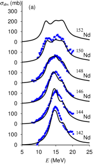
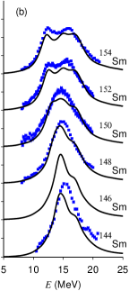
Figure 7: Photoabsorption cross sections in (a) Nd and (b) Sm isotopes as functions of photon energy YN11 . The Skyrme energy functional with the SkM* parameter set was used. The experimental data  car71 ; car74 are denoted by filled squares.

In the linear response equation (77), the system can oscillate without the external perturbation $v_{1}(\omega)=0$ (${\mathcal{V}}_{1}(\omega)=0$), at the eigenfrequencies $\omega=\omega_{n}$, Thus, the normal modes of excitation are obtained by solving the eigenvalue equation:

$$\begin{pmatrix}A&B\\ B^{*}&A^{*}\end{pmatrix}\begin{pmatrix}X^{n}\\ Y^{n}\end{pmatrix}=\omega_{n}\begin{pmatrix}1&0\\ 0&-1\end{pmatrix}\begin{pmatrix}X^{n}\\ Y^{n}\end{pmatrix}.$$ (163)

Solving this eigenvalue equation in the qp basis is the most common method for TDDFT to study elementary modes of excitation in superfluid nuclei. Because of numerical difficulties, most of current studies with Skyrme EDFs for deformed nuclei are restricted to axially deformed nuclei LPDVB10 ; Sto11 ; YN11 ; hfbtho .

We first calculate the qp states in the ground state in the 2D coordinate space assuming the axial symmetry. Then, all the necessary quantities are expressed in the qp representation. For deformed systems, the number of 2qp states becomes huge and we often need a further truncation of the 2qp space YN11 . In addition, the residual kernel associated with the long-range Coulomb part is neglected in the present calculation. The solutions of the eigenvalue equation (163) are obtained using the symmetrization procedure RS80 .

Heavy nuclei with open-shell configurations are supposed to have a superfluid character caused by the neutron-neutron and proton-proton pairing correlations. Here, we show results for Nd and Sm isotopes. The protons have finite pair densities for all these isotopes, while the neutron pair density vanishes for ¹⁴²Nd and ¹⁴⁴Sm which correspond to the neutron magic number $N=82$. These isotopes exhibit typical examples of the quantum phase transitions in their ground states, from spherical to prolate shapes, and simultaneously, from the normal to superfluid phases, as increasing the neutron number. Actually, the calculated ground states show a spherical shape for ^142,144Nd and ^144,146Sm, and a prolate shape for the others. The magnitude of deformation increases as the neutron number changes from 86 to 92.

In Fig. 7, the calculated photoabsorption cross sections for Nd and Sm isotopes are shown together with the available experimental data  car71 ; car74 . The dipole strength at discrete eigenenergies are smeared by the Lorentzian with a width $\gamma=2$ MeV. The GDR peak energies well agree with experimental values, and produces the deformation splitting in ^150,152Nd and ^152,154Sm. The GDR width calculated with $\gamma=2$ MeV is also in good accordance with the experimental values. The nice agreement on the broadening indicates that the smearing width $\gamma=2$ MeV has a good correspondence with the spreading width $\Gamma^{\downarrow}$ in these nuclei.

The isotopic dependence of the peak broadening is well reproduced, even for the transitional nuclei. The width for $N=82$ and 84 is calculated as $\Gamma\approx 4.5$ MeV, and it gradually increases to about 6 MeV for $N=88$ (¹⁴⁸Nd and ¹⁵⁰Sm), then the peak splitting becomes visible for $N\geq 90$ and 92. Here, the width $\Gamma$ is evaluated by fitting the calculated cross section with a Lorentz line. The broadening of the GDR was found to be well correlated with the nuclear quadrupole moments Oka55 ; Dan58 . Thus, it is interpreted as the mode-mode coupling effects to the low-lying collective modes  HW01 . In the present calculation, the mode coupling is not explicitly taken into account. However, the linear response based on the deformed state may implicitly include a part of the coupling effect. Figure 7 shows that the isotopic dependence can be well accounted for by the gradual increase of the ground-state deformation.

6 Large amplitude collective dynamics in shape coexistence

Low-energy collective modes of excitation in nuclei present unique features of the finite quantum systems. In contrast to giant resonances discussed in Sec. 5, the linear approximation is often insufficient for low-lying collective states in nuclei. The vibrational excitations should contain a strong anharmonicity when the stability matrix ${\mathcal{S}}$ has an eigenvalue close to zero, namely when the system is close to the critical point of the stability. This kind of situation occurs in many nuclei, especially for the quadrupole modes of excitation in a transitional situation such as shape phase transition (Fig. 7) and shape coexistence phenomena Woo92 ; HW11 . Therefore, we need to go beyond the linear regime for describing these nuclear phenomena of a large amplitude nature.

One of the unique features of the low-lying collective motion in nuclei is the fact that its character significantly changes from nucleus to nucleus. In addition, its structure is affected by an interplay between the pairing and deformation correlations, which often results in a spontaneous breaking of symmetry. Therefore, it is difficult to introduce an a priori assumption on the nature of the low-lying collective motion. Therefore, the theory presented in Sec. 4 is suitable to find optimal collective manifold which leads to a collective Hamiltonian. In this section, we show applications of the theory in Sec. 4.

In this section, we apply the method in Sec. 4.5 to description of low-lying spectra in neutron-deficient ⁶⁸Se. This nucleus shows a feature of the shape coexistence: The experimental data indicate that there exist rotational bands with different characters, which has been interpreted to be those with prolate and oblate shapes Fischer00 ; Fischer03 . The mixing property of the two bands are of significant interest, which influences the excitation spectra and transition probabilities. In this section, we show results only for ⁶⁸Se. The same analysis on ^70,72Se can be found in Ref. HNMM09 .

6.0.1 Pairing-plus-quadrupole model

The pairing-plus-quadrupole (P+Q) model is one of the most successful models that allows us to describe nuclear phenomena involving the quadrupole and pairing degrees of freedom. Baranger and Kumar studied the quadrupole motion in the P+Q model, assuming that the collective coordinates are given by the quadrupole deformations $(\beta,\gamma)$, and that the collective mass parameters are given by the cranking formula with phenomenological corrections BK65 . However, a study of the same model NWD99 reveals that, even at the minimum point of the potential, the self-consistent mass parameters and the property of normal modes are very different from those utilized by Baranger and Kumar. In the followings, we also adopt the Hamiltonian similar to the P+Q model and study the large amplitude collective motion in Se nuclei.

The P+Q model in the present study includes the quadrupole pairing and is given by

$$\begin{split}\hat{H}=&\sum_{k}\epsilon_{k}c_{k}^{\dagger}c_{k}-\frac{1}{2}\sum_{\tau=n,p}G_{0}^{(\tau)}(\hat{A}^{(\tau){\dagger}}\hat{A}^{(\tau)}+\hat{A}^{(\tau)}\hat{A}^{(\tau){\dagger}})\\ &-\frac{1}{2}\sum_{\tau=n,p}G_{2}^{(\tau)}\sum_{K}(\hat{B}_{2K}^{(\tau){\dagger}}\hat{B}_{2K}^{(\tau)}+\hat{B}_{2K}^{(\tau)}\hat{B}_{2K}^{(\tau)\dagger})-\frac{1}{2}\chi\sum_{K}\hat{D}_{2K}^{\dagger}\hat{D}_{2K},\end{split}$$ (164)

where $\epsilon_{k}$ are the spherical single-particle energies and the index $k$ denotes the set of quantum numbers $(njlm)$. The monopole pairing operator $\hat{A}^{(\tau){\dagger}}$, the quadrupole pairing operator $\hat{B}^{(\tau){\dagger}}$, and the mass quadrupole operator $\hat{D}^{{\dagger}}$ are defined by

$$\begin{split}\hat{A}^{(\tau){\dagger}}=&\sum_{(k>0)\in\tau}c_{k}^{{\dagger}}c_{\bar{k}}^{{\dagger}},\quad\quad\hat{B}_{2K}^{(\tau){\dagger}}=\sum_{k,l\in\tau}D_{2K}(kl)c_{k}^{{\dagger}}c_{l}^{{\dagger}},\\ \hat{D}_{2K}=&\sum_{k,l}D_{2K}(kl)c_{k}^{\dagger}c_{l},\end{split}$$ (165)

where $D_{2K}(kl)$ are the (dimensionless) quadrupole matrix elements, modified according to a prescription given by Baranger and Kumar BK65 . The model parameters are determined by adjusting the potential energy surface calculated with the Skyrme energy functional. Those values are found in Ref.  HNMM09 .

6.0.2 Results of MFHE

Figure 8: Calculated quantities on the collective path for ⁶⁸Se as functions of the triaxiality $\gamma$ HNMM09 . The axial deformation $\beta(q)$, the canonical collective coordinate $q$, the monopole pairing gaps $\Delta_{0}^{(\tau)}(q)$, the quadrupole pairing gaps $\Delta^{(\tau)}_{20}(q)$ and $\Delta^{(\tau)}_{22}(q)$, the collective potential $V(q)$, the collective mass $M(s(q))$, the lowest two eigenfrequencies of the MFHE $\omega^{2}(q)$, and the rotational moments of inertia ${\mathcal{J}}_{i}(q)$.

The Hartree-Bogoliubov (HB) approximation to the present P+Q Hamiltonian leads to two minima (HB states) in the potential energy surface, in ⁶⁸Se: The lowest minimum has an oblate shape ($\beta=0.3$) and the other minimum with a prolate shape ($\beta=0.26$) lies at energy about 400 keV higher than the oblate one. The obtained collective coordinate $q^{1}$ has a good one-to-one correspondence to the triaxial deformation parameter $\gamma$ in the quadrupole deformations $(\beta,\gamma)$ defined by

$$\beta\cos\gamma=\langle{\Psi(q^{1})}|\hat{D}_{20}|{\Psi(q^{1})}\rangle,\quad\beta\sin\gamma=\langle{\Psi(q^{1})}|(\hat{D}_{22}+\hat{D}_{2-2})|{\Psi(q^{1})}\rangle/\sqrt{2}.$$ (166)

This is seen in the top-right panel in Fig. 8. In Fig. 8, a variety of quantities calculated on the collective path are plotted as functions of $\gamma$. The mass parameter is defined with respect to the geometrical length $s$ in the $(\beta,\gamma)$ plane, $ds^{2}=\sqrt{d\beta^{2}+\beta^{2}d\gamma^{2}}$.

$$M_{s}^{-1}(q^{1})=\left(\frac{ds}{dq^{1}}\right)^{2}\bar{B}^{11}=\left\{\left(\frac{d\beta}{dq^{1}}\right)^{2}+\beta^{2}\left(\frac{d\gamma}{dq^{1}}\right)^{2}\right\}\bar{B}^{qq}.$$ (167)

In the prolate and oblate minima, the lowest modes of excitation in the MFHE correspond to the gamma vibrations, and the second lowest to the beta vibrations. The frequency $\omega$, then, turns into imaginary in the triaxial region ($10^{\circ}<\gamma<50^{\circ}$). The imaginary frequency causes no problem in the solution of the MFHE. We also calculate the moments of inertia by solving the Thouless-Valatin equations TV62 on the collective path, which gives ${\mathcal{J}}_{k}(q)$, $k=x,y,z$. These are also shown in the bottom-right panel in Fig. 8. They have a characteristic feature similar to the moments of inertia of the irrotational fluid RS80 .

6.0.3 Collective Hamiltonian

In the total kinetic energy, the position-dependent rotational energy is added to the one of the one-dimensional shape vibration described by the coordinate $q^{1}$.

$$T=\frac{1}{2}\bar{B}^{ij}(q^{1})p_{i}p_{j}$$ (168)

where $i,j=1,\cdots,4$. Here, $(p_{2},p_{3},p_{4})$ are the total angular momentum $(I_{x},I_{y},I_{z})$, and $\bar{B}^{ij}=\delta^{ij}(\bar{B}^{11},{\mathcal{J}}_{x}^{-1},{\mathcal{J}}_{y}^{-1},{\mathcal{J}}_{z}^{-1})$. The kinetic energy term is requantized by means of the Pauli prescription:

$$\hat{T}= -\frac{1}{2}\sum_{ij}|G(q^{1})|^{-\frac{1}{2}}\frac{\partial}{\partial q^{i}}|G(q^{1})|^{\frac{1}{2}}\bar{B}^{ij}(q^{1}))\frac{\partial}{\partial q^{j}}$$

$$= -\frac{1}{2}\frac{\partial}{\partial q^{1}}\bar{B}^{11}(q^{1})\frac{\partial}{\partial q^{1}}-\frac{1}{4}\frac{\partial G}{\partial q^{1}}\frac{\bar{B}^{11}(q^{1})}{G(q^{1})}\frac{\partial}{\partial q^{1}}+\sum_{k=x,y,z}\frac{\hat{I}^{2}_{k}}{2{\mathcal{J}}_{k}(q^{1})},$$ (169)

where $G(q)=\bar{B}_{11}(q^{1}){\mathcal{J}}_{x}(q^{1}){\mathcal{J}}_{y}(q^{1}){\mathcal{J}}_{z}(q^{1})$ is the determinant of the metric $\bar{B}_{ij}(q^{1})$. The three components $\hat{I}_{k}$ of the angular momentum operator are defined with respect to the principal axes $(x,y,z)$ associated with the intrinsic (moving-frame) state $|{\phi(q^{1})}\rangle$.

The collective Schrödinger equation is thus given, with $q^{1}$ replaced by $q$ hereafter, as

$$(\hat{T}+V(q))\Psi_{IMn}(q,\Omega)=E_{I,n}\Psi_{IMn}(q,\Omega),$$ (170)

where $\Psi_{IMn}(q,\Omega)$ represents the collective wave function in the laboratory frame. It is a function of the collective coordinate $q$ and the three Euler angles $\Omega$, and specified by the total angular momentum $I$, its projection $M$ on the laboratory $z$-axis, and the index $n$ distinguishing different quantum states having the same $I$ and $M$. Using the rotational wave functions ${\mathcal{D}}^{I}_{MK}(\Omega)$, the collective wave functions in the laboratory frame is written as

$$\Psi_{IMn}(q,\Omega)= \sum_{K=0}^{I}\Phi_{IKn}(q)\langle\Omega|IMK\rangle,$$ (171)

$$\langle\Omega|IMK\rangle= \sqrt{\frac{2I+1}{16\pi^{2}(1+\delta_{K0})}}({\mathcal{D}}^{I}_{MK}(\Omega)+(-)^{I}{\mathcal{D}}^{I}_{M-K}(\Omega))$$ (172)

where the sum in Eq. (171) is restricted to even $K$. Here, $\Phi_{IKn}(q)$ represents the shape vibrational motion described by the coordinate $q$.

Normalization of the vibrational part of the collective wave functions is given by

$$\int d\tau^{\prime}\sum_{K=0}^{I}\Phi^{\ast}_{IKn}(q)\Phi_{IKn^{\prime}}(q)=\delta_{nn^{\prime}}$$ (173)

where the volume element is

$$d\tau=d\tau^{\prime}d\Omega=\sqrt{|G(q)|}dqd\Omega.$$ (174)

The boundary conditions for the collective Schrödinger equation (170) can be specified by projecting the obtained collective path onto the $(\beta,\gamma)$ plane and by using the symmetry properties of the Bohr-Mottelson collective Hamiltonian KB67 .

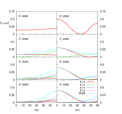
Figure 9: Calculated spectra and $B(E2)\downarrow$ in units of e²fm⁴ (left) and the collective wave functions as functions of $\gamma$ (right). The figures are taken from Ref. HNMM09

6.0.4 Discussion: Rotational localization

In the left panel of Fig. 9, excitation spectra and $B(E2)$ values calculated for ⁶⁸Se are displayed together with experimental data. The calculation yields two rotational bands, which qualitatively agrees with experiment. The calculated ground and excited bands have oblate and prolate characters, respectively, however, there is strong shape mixing, especially at low spins. Note that the calculated $0_{2}^{+}$ state is located above the $2_{2}^{+}$ state. We find that this significant rise of the $0_{2}^{+}$ excitation energy is due to the oblate-prolate shape mixing in the $0^{+}$ states, which is much stronger than that of the $2^{+}$ states. It would be very interesting to identify the $0_{2}^{+}$ experimentally.

The strong shape mixing in the $0^{+}$ states can be confirmed by examining the vibrational wave functions displayed in the right panel of Fig. 9. Since the potential barrier between the two minima is only 400 keV high along the collective path, this strong mixing is reasonable. In fact, the unusual behavior of the excited $0^{+}$ state suggests an intermediate situation between the oblate-prolate shape coexistence and the $\gamma$-unstable model by Wilet and Jean WJ56 .

It is quite interesting to notice that the shape mixing becomes weak as the angular momentum increases. The collective wave functions of the the $4^{+}$ and $6^{+}$ states tend to localize in the region near either the oblate or the prolate shape. Namely, it becomes more appropriate to characterize the $4^{+}$ and $6^{+}$ states as oblate-like or prolate-like. We have analyzed dynamical origin of this trend and found that the rotational energy plays a crucial role in determining localization of the collective wave function. Therefore, this effect may be called “rotational localization of collective wave function” or “rotational hindrance of shape mixing” HNMM09 .

6.1 Further developments

6.1.1 Multi-dimensional collective submanifold

The 1D collective path for ⁶⁸Se is obtained by following the lowest eigensolution of the MFHE. Figure 10 shows an embedded collective path in the $(\beta,\gamma)$ plane. However, the frequency of the second lowest solution is only $1\sim 1.5$ MeV higher than the lowest one (Fig. 8). Thus, the extension from 1D to 2D may be important. We often encounter similar situations which suggest importance of the multi-dimensional collective submanifold. Numerically, this is a challenging task, because we need to search for self-consistent solutions of the MFHE in the 2D or higher-dimensional hypersurface. The technical developments for the multi-dimensional collective submanifold is an important future subject.

In recent papers HSNMM10 ; SH11 ; HSYNMM11 , the collective Hamiltonian with the 2D shape degrees has been constructed assuming the one-to-one correspondence between the collective coordinates $(q^{1},q^{2})$ and $(\beta,\gamma)$, combined with following approximations:

1. The collective submanifold is determined by the minimization with respect to the mass quadrupole operators, neglecting the self-consistency between Eqs. (155) and (156).

2. In the MFHE, the curvature terms are neglected.

The eigensolutions of the MFHE are used to calculate the collective mass parameters, $\bar{B}^{ij}=f^{i}_{,\alpha}f^{j}_{,\beta}\widetilde{B}^{\alpha\beta}$. The inclusion of the 2D shape degrees of freedom turns out to be qualitatively consistent with the 1D calculation in Fig. 9, but further improve the results in comparison with experiments HSNMM10 .

6.1.2 Applications to modern energy functionals

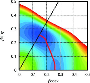
Figure 10: The collective path for ⁶⁸Se in the $(\beta,\gamma)$ plane. The contour plot shows the result of the energy minimization with the constraints on the mass quadrupole operators, $D_{20}$ and $D_{22}+D_{2-2}$.

It is also highly desired to apply the method to realistic modern energy functionals, such as Skyrme, Gogny, and covariant energy functionals. This requires a developments of the code for MFHE without the axial symmetry restriction.

Adopting the similar approximations mentioned above, there are numerous recent works, in the Skyrme energy functionals PQSL04 ; PR09 the Gogny energy functionals LGD99 ; Del10 , and the covariant EDFs Nik09 ; Li09 , to construct the collective Bohr Hamiltonian with the microscopic inputs. However, the collective mass parameters are further approximated by the Inglis-cranking formula. Since this cranking approximation has a well-known defect leading to a disagreement with experiments, the phenomenological scaling to increase the collective mass by roughly $30-40$ %, is often adopted. This comes from the fact that the cranking formula neglects the time-odd mean fields RS80 . Therefore, the replacement of the cranking mass by the MFHE mass should solve this problem.

The MFHE with the Skyrme energy functional has been applied to studies of Cr isotopes with the above approximations and a restriction to the 1D shape degree YH11 . In a very recent work HLNNV12 , a hybrid model, combining the covariant EDF method with the MFHE in the P+Q model, has been investigated. Namely, the potential energy surface is calculated by the covariant EDF and the collective mass parameters are estimated by the help of MFHE in the P+Q model. The model shows a significant improvement in the low-lying spectra in $\gamma$-soft nuclei of Xe and Ba isotopes. These results suggest a promising future of the MFHE in the energy functional approaches.

7 Summary

Intensive studies in density functional theories (DFT) in recent years have produced numerous new results and new insights into nuclear structure. It is beyond the scope of the present paper to review all of these developments. In this paper, we mainly focus our discussion on the basic concepts of the nuclear DFT and applications of the time-dependent DFT (TDDFT).

The nucleus is a self-bound isolated system without an external potential. This produces a situation different from many-electron systems with the external Coulomb potentials. Therefore, we need modify the original arguments of the DFT, such as the Hohenberg-Kohn theorem. In Sec. 2, we presented a justification based on the Hohenberg-Kohn theorem modified for the wave packet. It can be formulated with the Kohn-Sham scheme as well. To incorporate effects of the nucleonic pair condensation, the density functional should be generalized to include the pair density (abnormal density) in addition to the normal density. This can be done with the generalized scheme by Bogoliubov. The TDDFT was also established, in the same manner as the Hohenberg-Kohn, by the one-to-one correspondence between the potential and density depending on time.

Most applications of the TDDFT are performed in the perturbative linear response regime. Even in the linear regime, because of the complexity of the EDFs of nuclei, it is computationally very demanding to perform the numerical calculations and requires significant works for its program coding. There are several approaches to the linear-response calculations, each of which has an advantage and disadvantage. This has been discussed in details in Sec. 3. As a feasible approach, we have proposed the finite amplitude method (FAM). The FAM only requires a minor modification of the existing program of the stationary calculation for the nuclear ground-state properties.

The nucleus is also known to show many collective phenomena at low energies which are not able to be described by the linear-response theory. A typical example is given by the fission of heavy nuclei, and by the shape phase transition and the shape coexistence. For this purpose, we have presented a theory of a decoupled collective space inside the large TDDFT phase space in Sec. 4. In case that the collective motion of interest is slow relative to the other intrinsic degrees of freedom, self-consistent solutions of the moving-frame harmonic equation (MFHE) with the constraint minimization of the EDF provide microscopic determination of the collective variables and the collective Hamiltonian.

In Sec. 5 and Sec. 6, we presented selected results of recent studies with the TDDFT on nuclear dynamics in the linear-response regime and beyond the linear regime. Properties of giant resonances in nuclei, especially those of the giant dipole resonance (GDR), have been studied with the Skyrme energy functionals. Currently available EDFs are able to reproduce the GDR in heavy nuclei, however, have a problem for that in light nuclei. We also presented the applications of the MFHE to shape coexistence phenomena in ⁶⁸Se. The calculation suggests a rotation-induced localization of the collective wave functions, which produces the oblate-prolate shape coexistence in this nucleus.

An interplay between theory and experiment has been and will be providing deeper understanding of the nuclear quantum many-body problem. To develop a comprehensive predictive theory of the nucleus to answer fundamental scientific questions, still significant components are missing from our current understanding. Some of these missing parts can be addressed only by the large-scale numerical simulations of nuclear systems. The petascale- and of future exascle-computing platforms is expected to pave the way to this goal.

I thank all my collaborators working together on subjects in this paper, including P. Avogadro, G. Do Dang, S. Ebata, T. Inakura, N. Hinohara, M. Matsuo, K. Matsuyanagi, K. Sato, N. Walet, K. Yabana, and K. Yoshida. Part of the work was carried out under Grant-in-Aid for Scientific Research(B) No. 21340073 and Innovative Areas No. 20105003. The numerical calculations were performed in part on the RIKEN Integrated Cluster of Clusters (RICC), and on PACS-CS and T2K in University of Tsukuba.

References

- (1) E. Rutherford, Phil. Mag. 21 (1911), 669.
- (2) H. Geiger and E. Marsden, Proc. Roy. Soc. London A82 (1909), 495; H. Geiger, Proc. Roy. Soc. London A83 (1910), 492.
- (3) N. Bohr, Phil. Mag. 26 (1913), 1.
- (4) A. Bohr and B. R. Mottelson, Nuclear Structure, vol. 1 (W. A. Benjamin, 1969).
- (5) S. C. Pieper and R. B. Wiringa, Ann. Rev. Nucl. Part. Sci. 51 (2001), 53.
- (6) A. Nogga, P. Navratil, B. R. Barrett, and J. P. Vary, \PRC73,2006,064002.
- (7) H. Kümmel, K. H. Lührmann, and J. G. Zabolitzky, \PRP36,1978, 1.
- (8) R. J. Bartlett and M. Musiał, Rev. Mod. Phys. 79 (2007), 291.
- (9) M. Wloch, D. J. Dean, J. R. Gour, M. Hjorth-Jensen, K. Kowalski T. Papenbrock, and P. Piecuch, \PRL94,2005,212501.
- (10) UNEDF SciDAC collaboration (http://www.unedf.org/).
- (11) J. W. Negele, Rev. Mod. Phys. 54 (1982), 913.
- (12) T. Nakatsukasa, J. Phys. Conf. Ser. 302 (2011), 012050.
- (13) P. Hohenberg and W. Kohn, \PR136,1964,B864.
- (14) W. Kohn and L. J. Sham, \PR140,1965,A1133.
- (15) M. Bender, P. H. Heenen, and P.-G. Reinhard, Rev. Mod. Phys. 75 (2003), 121.
- (16) D. Lunney, J. M. Pearson, and C. Thibault, Rev. Mod. Phys. 75 (2003), 1021.
- (17) M. Galitskii, JETP 7 (1958), 104.
- (18) E. Runge and E. K. U. Gross, \PRL52, 2984,997.
- (19) P. Ring and P. Schuck, The nuclear many-body problem, (Springer-Verlag, 1980).
- (20) J. Engel, \PRC75,(2007,014306.
- (21) B. Giraud, \PRC77,2008,014311; ibid. 78 (2008), 014307.
- (22) B. Giraud, B. K. Jennings, and B. R. Barrett, \PRA78,2008,032507.
- (23) M. Levy, Proc. Natl. Acad. Sci. U.S.A. 76 (1979), 6062.
- (24) A. Bohr and B. R. Mottelson, Nuclear Structure, vol. 2 (W. A. Benjamin, 1975).
- (25) S. Ebata, T. Nakatsukasa, T. Inakura, K. Yoshida, Y. Hashimoto, and K. Yabana, \PRC82,2010,034306.
- (26) N. N. Bogoliubov, JETP 7 (1958), 41.
- (27) J.-P. Blaizot and G. Ripka, Quantum Theory of Finite Systems, (MIT Press,1986).
- (28) J. Dobaczewski, H. Flocard, and J. Treiner, \NPA422,1984,103
- (29) D. Vautherin and D. M. Brink, \PRC5,1972,626.
- (30) J. Dechargé and D. Gogny, \PRC21,1980,1568.
- (31) S. Shlomo and G. Bertsch, \NPA243,1975,507.
- (32) A. Zangwill and P. Soven, \PRA21,1980,1561
- (33) K. Yabana and G. F. Bertsch, \PRB54,1996,4484.
- (34) T. Nakatsukasa and K. Yabana, J. Chem. Phys. 114 (2001), 2550.
- (35) T. Nakatsukasa and K. Yabana, \PRC71,2005,024301.
- (36) K. Yabana, Y. Kawashita, T. Nakatsukasa, and J.-I. Iwata, Charged Particle and Photon Interactions with Matter: Recent Advances, Applications, and Interfaces (CRC Press Taylor & Francis), pp. 65-86.
- (37) D. Neuhasuer and M. Baer, J. Chem. Phys. 90 (1989), 4351.
- (38) M.S. Child, Mol. Phys. 72 (1991), 89.
- (39) T. Nakatsukasa, T. Inakura, and K. Yabana, \PRC76,2007,024318.
- (40) P. Avogadro and T. Nakatsukasa, \PRC84,2011,014314.
- (41) M. Stoitsov, M. Kortelainen, T. Nakatsukasa, C. Losa, and W. Nazarewicz, \PRC84,2011,041305.
- (42) G. Do Dang, A. Klein, and N. R. Walet, \PRP335,2000, 93.
- (43) A. Kuriyama, K. Matsuyanagi, F. Sakata, K. Takada, and M. Yamamura, \PTP141,2001,1.
- (44) T. Nakatsukasa, N.R. Walet, and G. Do Dang, \PRC61,1999,014302.
- (45) M. Matsuo, T. Nakatsukasa, and K. Matsuyanagi, \PTP103,2000,959.
- (46) N. Hinohara, T. Nakatsukasa, M. Matsuo, and K. Matsuyanagi, \PTP117,2007,451.
- (47) N. Hinohara, T. Nakatsukasa, M. Matsuo, and K. Matsuyanagi, \PTP119,2008,59.
- (48) N. Hinohara, T. Nakatsukasa, M. Matsuo, and K. Matsuyanagi, \PRC80,2009,014305.
- (49) H. Flocard and S. E. Koonin and M. S. Weiss, \PRC17,1978,1682.
- (50) T. Inakura, T. Nakatsukasa, and K. Yabana, \PRC80,2009,044301.
- (51) K. F. Liu and N. van Giai, \PLB65,1976,23.
- (52) I. Hamamoto, H. Sagawa, and X. Z. Zhang, \PRC57,1998,R1064.
- (53) H. Sagawa, \PTPS142,2001,1.
- (54) M. Matsuo, \NPA696,2001,371.
- (55) Z. H. Levine and P. Soven, \PRA29,1984,625.
- (56) P. Bonche and S. Koonin and J. W. Negele, \PRC13,1976,1226.
- (57) J. P. Blaizot, \PRP64,1980,171.
- (58) T. Nakatsukasa, S. Mizutori, and K. Matsuyanagi, \PTP87,1992,607.
- (59) T. Nakatsukasa, K. Matsuyanagi, S. Mizutori, and Y. R. Shimizu, \PRC53,1996,2213.
- (60) W. H. Press, S. A. Teukolsky, W. T. Vetterling, and B. P. Flannery, Numerical Recipes in C, Cambridge University Press, 2007).
- (61) S. C. Eisenstat, H. C. Elman, and M. H. Schultz, SIAM J. Numer. Anal. 20 (1983), 345.
- (62) S.-L. Zhang, SIAM J. Sci. Comput. 18 (1997), 537.
- (63) H. A. Van der Vorst, SIAM J. Sci. Comput. 13 (1992), 631.
- (64) M. H. Gutknecht, SIAM J. Sci. Comput. 14 (1993), 1020.
- (65) Moe Thuthu and S. Fujino, ASCM 5801 (2008), 108.
- (66) J. Toivanen, B. G. Carlsson, J. Dobaczewski, K. Mizuyama, R. R. Rodríguez-Guzmán, P. Toivanen, and P. Veselý, \PRC81,2010,034312.
- (67) M. A. Elkin, B. S. Ishkhanov, I. M. Kapitonov, E. I. Lileeva, and E. V. Shirokov, Phys. Atom. Nucl. 67 (2004), 4.
- (68) V. V. Varlamov, M. E. Stepanov, and V. V. Chesnokov, Bull. Russian Acad. Sci. Phys. Ser. 67 (2003) 724.
- (69) J. Wambach, Rep. Prog. Phys. 51 (1988), 989.
- (70) M. N. Harakeh and A. van der Woude, Giant resonances (Oxford University Press, 2001).
- (71) J. Terasaki and J. Engel, \PRC74,2006,044301.
- (72) T. Sil, S. Shlomo, B. K. Agrawal, and P.-G. Reinhard, \PRC73,2006,034316.
- (73) A. Leprêtre, H. Beil, R. Bergère, P. Carlos, A. Veyssière, and M. Sugawara \NPA175,1971,609.
- (74) A. Leprêtre, H. Beil, R. Bergère, P. Carlos, A. De Miniac, A. Veyssière, and K. Kernbach, \NPA219,1974,39.
- (75) S. N. Beljaev and V. A. Semenov, Izv. Ross. Akad. Nauk, SSSR, Ser. Fiz. 55 (1991), 953.
- (76) C. Losa, A. Pastore, T. Døssing, E. Vigezzi, and R. A. Broglia, \PRC81,2010,064307.
- (77) K. Yoshida and T. Nakatsukasa, \PRC83,2011,021304.
- (78) M.V. Stoitsov, J. Dobaczewski, W. Nazarewicz, and P. Ring, Comp. Phys. Comm. 167 (2005), 43.
- (79) I. Stetcu, A. Bulgac, P. Magierski, and K. J. Roche, \PRC84,2011,051309.
- (80) P. Carlos et al., \NPA172, 1971,437.
- (81) P. Carlos et al., \NPA225,1974,171.
- (82) K. Okamoto, \PTP15,1955,75; \PR110,1958,143.
- (83) M. Danos, \NP5,1958,23.
- (84) J.L Wood, K Heyde, W Nazarewicz, M Huyse, and P van Duppen, \PRP215,1992, 101.
- (85) K. Heyde and J. L. Wood, Rev. Mod. Phys. 83 (2011), 1467.
- (86) S. M. Fischer et al., \PRL84,2000, 4064.
- (87) S. M. Fischer et al., \PRC67,2003,064318.
- (88) M. Baranger and K. Kumar, \NP62,1965,113; \NPA110,1968, 490; ibid. 110 (1968), 529; ibid. 122 (1968), 241; ibid. 122 (1968), 273.
- (89) D. J. Thouless and J. G. Valatin, \NP31,1962,211.
- (90) N. Hinohara, T. Nakatsukasa, M. Matsuo, and K. Matsuyanagi, \PTP115,2006,567.
- (91) K. Kumar and M. Baranger, \NPA92,1967,608.
- (92) L. Wilets and M. Jean, \PR102,1956, 788.
- (93) N. Hinohara, K. Sato, T. Nakatsukasa, M. Matsuo, and K. Matsuyanagi, \PRC82,2010,064313.
- (94) K. Sato and N. Hinohara, \NPA849,2011,53.
- (95) N. Hinohara, K. Sato, K. Yoshida, T. Nakatsukasa, M. Matsuo, and K. Matsuyanagi, \PRC84,2011,061302.
- (96) L. Próchniak, P. Quentin, D. Samsoen, and J. Libert, \NPA730,2004,59.
- (97) L. Próchniak and S. G. Rohoziński, J. Phys. G 36 (2009), 123101.
- (98) J. Libert, M. Girod, and J.-P. Delaroche, \PRC60,1999,054301.
- (99) J.-P. Delaroche et al., \PRC81,2010,014303.
- (100) T. Niks̆ić et al., \PRC79,2009,034303.
- (101) Z. P. Li et al., \PRC79,2009,054301.
- (102) K. Yoshida and N. Hinohara, \PRC83,2011,061302.
- (103) N. Hinohara, Z. P. Li, T. Nakatsukasa, T. Nikšić, and D. Vretenar, \PRC85,2012,024323.