Pilot, Rollout and Monte Carlo Tree Search Methods for Job Shop Scheduling

Abstract

Greedy heuristics may be attuned by looking ahead for each possible choice, in an approach called the rollout or Pilot method. These methods may be seen as meta-heuristics that can enhance (any) heuristic solution, by repetitively modifying a master solution: similarly to what is done in game tree search, better choices are identified using lookahead, based on solutions obtained by repeatedly using a greedy heuristic. This paper first illustrates how the Pilot method improves upon some simple well known dispatch heuristics for the job-shop scheduling problem. The Pilot method is then shown to be a special case of the more recent Monte Carlo Tree Search (MCTS) methods: Unlike the Pilot method, MCTS methods use random completion of partial solutions to identify promising branches of the tree. The Pilot method and a simple version of MCTS, using the $\varepsilon$-greedy exploration paradigms, are then compared within the same framework, consisting of 300 scheduling problems of varying sizes with fixed-budget of rollouts. Results demonstrate that MCTS reaches better or same results as the Pilot methods in this context.

1 Introduction

In quite a few domains related to combinatorial optimization, such as constraint solving [1], planning or scheduling [2], software environments have been designed to achieve good performances in expectation over a given distribution of problem instances. Such environments usually rely on a portfolio of heuristics, leaving the designer with the issue of finding the best heuristics, or the best heuristics sequence, for his particular distribution of problem instances.

The simplest solution naturally is to use the default heuristics, assumedly the best one on average on all problem instances. Another approach, referred to as Pilot or rollout method, iteratively optimizes the option selected at each choice point [3, 4], while sticking to the default heuristics for other choice points. Yet another approach, referred to as Monte-Carlo Tree Search (MCTS) [5] and at the origin of the best current computer-Go players [6], has been proposed to explore the search space while addressing the exploration versus exploitation dilemma in a principled way; as shown by [7], MCTS provides an approximation to optimal Bayes decision. The MCTS approach, rooted in the multi-Armed bandit (MAB) setting [8], iteratively grows a search tree through tree walks. For each tree walk, in each node (choice point) the selection of the child node (heuristics) is handled as a MAB problem; the search tree thus asymmetrically grows to explore the most promising tree paths (the most promising sequences of heuristics).

Whereas increasingly used today in sequential decision making algorithms including games [9, 10], to our best knowledge MCTS methods have rarely been used within the framework of combinatorial optimization, with the recent exception of [11]. This paper investigates the application of MCTS to job-shop scheduling, an NP-hard combinatorial optimization problem. As each job-shop scheduling problem instance defines a deterministic optimization problem, the standard upper confidence bound applied to tree (UCT) framework used in [11] does not apply. More precisely, the sought solution is the one with best payoff (as opposed to the one with best payoff on average); the MAB problem nested in the UCT thus is a max $k$-armed bandit problem [12, 9]. Along this line, the randomized aspects in UCT must be addressed specifically to fit deterministic problems. Specifically, a critical difficulty lies in the randomized default handling of the choice points which are outside the current search tree (in contrast, these choice points are dealt with using the default heuristics in the pilot methods). Another difficulty, shared with most MCTS applications, is to preserve the exploration/ exploitation trade-off when the problem size increases. A domain-aware randomized default handling is proposed in this paper, supporting a MCTS-based scheduling approach called Monte-Carlo Tree Scheduling (MCS). MCS is empirically validated, using well established greedy heuristics and the pilot methods based on these heuristics as baselines. The empirical evidence shows that Pilot methods significantly outperform the best-known default heuristics; MCS significantly outperforms on the Pilot methods for small problem sizes. For larger problem sizes, however, MCS is dominated by the best Pilot methods, which is partly explained from the experimental setting as the computational cost of the Pilot methods is about 4 times higher than that of the MCS one. That is, heuristic scheduling is more costly than random scheduling.

The paper is organized as follows. Job-shop scheduling is introduced in Section 2, together with some basic greedy algorithms based on domain-specific heuristics called dispatching rules. The generic pilot method is recalled in section 3. The general MCTS ideas are introduced in section 4; its adaptation to the job-shop scheduling problem is described and an overview of MCS is given. and together with its application to combinatorial problems, and to the job-shop scheduling problem. Section 5 is devoted to the empirical validation of the proposed approach. After describing the experimental setting, the section reports on the MCS results on different problem sizes, with the dispatching rules and the Pilot methods as baselines. The paper concludes with a discussion of these results and some perspectives for further research.

2 Job Shop Scheduling and priority dispatching rules

Scheduling is the sequencing of the order in which a set of jobs $j\in J:=\{1,..,n\}$ are processed through a set of machines $a\in M:=\{1,..,m_{j}\}$. In a job shop, the order in which a job is processed through the machines is predetermined. In a flow shop this order is the same for all jobs, and in a open shop the order is arbitrary. We will consider here only the job shop, where the jobs are strictly-ordered sequences of operations. A job can only be performed by one type of machine and each machine processes one job at a time. Once a job is started it must be completed. The performance metric for scheduling problems is generally based on flow or dues date. Here we will consider the completion time for the last job or the so called makespan.

Each job has a specified processing time $p(j,a)$ and the order through the machines is given by the permutation vector $\sigma$ ($\sigma(j,i)$ is the $i^{th}$ machine for job $j$). Let $x(j,a)$ be the start time for job $j$ on machine $a$, then

$$x(j,\sigma(j,i))\geq x(j,\sigma(j,i-1)+p(j,\sigma(j,i-1))\quad j\in\{1,..,n\},\;i\in\{2,..,m_{j}\}$$ (1)

The disjunctive condition that each machine can handle at most one job at a time is the following:

$$x(j,a)\geq x(k,a)+p(k,a)\quad\textrm{or}\quad x(k,a)+p(k,a)\geq x(j,a)$$ (2)

for all $j,k\in J,j\neq k$ and $a\in M$. The makespan can then be formally defined as

$$z=\max\{x(j,\sigma(j,m_{j}))+p(j,m_{j})\;|\;j\in J\}.$$ (3)

Smaller problems can be solved using a specialized branch and bound procedure [13] and an algorithmic implementation may be found as part of LiSA [14]. Jobs up to 14 jobs and 14 machines can still be solved efficiently, but at higher dimensions, the problems rapidly become intractable. Several heuristics have been proposed to solve job shop problems when their size becomes too large for exact methods. One such set of heuristics are based on dispatch rules, i.e. rules to decide which job to schedule next based on the current state of all machines and jobs. A survey of over 100 such rules may be found in [15]. Commonly used priority dispatch rules have been compared on a number of benchmark problems in [16]. When considering the makespan as a performance metric, the rule that selects a job which has the Most WorK Remaining (MWKR, the job with the longest total remaining processing time) performed overall best. It was followed by the rule that selects a job with the Shortest Processing Time (SPT), and by the rule that selects a job which the Least Operation Number (LOPN). These rules are among the simplest ones, and are by no means optimal. However, only these 3 rules will be considered in the remaining of this paper. In particular, experimental results of the corresponding 3 greedy algorithms can be found in Section 5.

The simplest way to use any of these rules is to embed them in a greedy algorithm: the jobs are processed in the order given by the repeated application of the chosen rule. Algorithm 1 gives the pseudo-code of such an algorithm. The variable $t_{j}$ represents which machine is next in line for job $j$ (more precisely machine $\sigma(j,t_{i})$). When starting with an empty schedule, one would set $t_{j}\leftarrow 1$ for $j\in J$ and ${\cal S}=\emptyset$. At each step of the algorithm, one job is chosen according to the dispatching rule R (line 1), and the job is scheduled on the next machine in its own list, i.e., the pair (job, machine) is added to the partial schedule $\cal S$ (line 1) ($\oplus$ denotes the concatenation of two lists).

input : Partial sequence ${\cal S}_{0}$, ${\mathbf{t}}=(t_{1},\ldots,t_{n})$, and heuristic R

output : An objective to maximize, for example negative makespan

while $\exists j\in J\;;\;t_{j}<m_{j}$ do $b=\mbox{\bf R}({\cal S},t_{j}\;;t_{j}<m_{j})$ ;  // Apply R to current partial schedule, get next job

${\cal S}\leftarrow{\cal S}\oplus\{(b,\sigma(b,t_{b}))\}$ ;  // Schedule job on its next machine

$t_{b}\leftarrow t_{b}+1$ ;  // Point to next machine for job $b$

end

Algorithm 1 Greedy (Pilot) heuristic

3 Pilot Method

The pilot method [3, 17] or equivalently the Rollout algorithm [18] can enhance any heuristic by a simple look-ahead procedure. The idea is to add one-step look-ahead and hence apply greedy heuristics from different starting points. The procedure is applied repeatedly, effectively building a tree. This procedure is not unlike strategies used in game playing programs, that search a game trees for good moves. In all cases the basic idea is to examine all possible choices with respect to their future advantage. An alternative view is that of a sequential decision problem or dynamic programming problem where a solution is built in stages, whereby the components (in our cases the jobs) are selected one-at-a-time. The first $k$ components form a so called $k$-solution [18]. In the same way as a schedule was built in stages in Algorithm 1, where the $k$-solution is the partial schedule ${\cal S}$. However, for the Pilot method the decisions made at each stage will depend on a look-ahead procedure. The Pilot method is then described in Algorithm 2. The algorithm may seem a little more complicated than necessary, however, as will be seen in the next section this algorithm is a special case of Monte Carlo tree search. The heuristic rollout is performed $B$ times and each time adding a node to the tree. Clearly if all nodes can be connected to a terminal node, the repetition may be halted before the budget $B$ is reached. This is not shown here for clarity. Furthermore, a new leaf on the tree is chosen such that those closer to the root have priority else branches are chosen arbitrarily with equal probability. In some version of the Pilot method, the tree is not expanded breadth first manner but with some probability allows for depth first search. This would be equivalent to executing line 2 with some probability. This is also commonly used in MCTS and is called progressive widening.

input : Budget $B$, partial sequence ${\cal S}_{0}$, ${\mathbf{t}}=(t_{1},\ldots,t_{n})$, and heuristic R

output : Decision, job to dispatch next $b$

$root\leftarrow node$ ; // initialize the root node

$node.n\leftarrow 0,node.{\mathbf{t}}\leftarrow{\mathbf{t}},node.child\leftarrow\emptyset$;

for $n\leftarrow 1$ to $B$ do ${\cal S}\leftarrow{\cal S}_{0}$ ;  // set state to root node state and climb down the tree

while $node.child\neq\emptyset$ do for $j\in J;node.t_{j}<m_{j}$ do if $node.n=0$ then $Q(j)=\infty$ else $Q(j)=U(0,1)$ ;  // random value between 0 and 1

end end $j^{\prime}=\arg\max_{j\in J;t_{j}<m_{j}}Q(j)$ ;  // largest $Q$ value, break ties randomly

${\cal S}\leftarrow{\cal S}\oplus\{(j^{\prime},\sigma(j^{\prime},t_{j^{\prime}}))\}$ ;  // dispatch job $j^{\prime}$

end ; // expand node if possible, i.e. ${\cal S}$ is not the complete schedule

for $j\in J;node.t_{j}<m_{j}$ do $node.child[j].parent\leftarrow node$ ;  // keep pointer to parent node

$node.child[j].child\leftarrow\emptyset$ ;  // this node has not been expanded

$node.child[j].n\leftarrow 0$ ;  // and has not been rolled out

$node.child[j].{\mathbf{t}}\leftarrow node.{\mathbf{t}}$ ;  // copy machine counter from parent node

$node.child[j].t_{j}\leftarrow node.t_{j}+1$ ;  // increment machine counter for job

end $R=$ Rollout (${\cal S},node[{\cal S}].{\mathbf{t}},{\bf R}$) ;  // Complete the solution via Pilot heuristic

repeat propagate result of rollout up the tree $node.n\leftarrow node.n+1$ ;  // number of visits incremented by one

$node.Q\leftarrow\max(node.Q,R)$ ;  // best found solution

$node\leftarrow node.parent$ ;  // climb up the tree to parent node

until $node\neq root$ ;

end $\arg\max_{j\in J;t_{j}<m_{j}}root.child(j).Q$

Algorithm 2 Pilot or rollout algorithm

2

2

The greedy algorithm 1 is then used as the Rollout algorithm on line 2. As will be seen in the following section, the key difference between the MCTS and Pilot method is in the way a node is found to expand in the tree and the manner in which a rollout is performed. Other details of the Algorithm 2 will also become clearer.

4 MCTS for Combinatorial Optimization

4.1 Monte Carlo Tree Search

Monte-Carlo Tree Search inherits from the so-called Multi-Armed Bandit (MAB) framework [8]. MAB considers a set of independent $k$ arms, each with a different payoff distribution. Here each arm corresponds to selecting a job to be dispatched and the payoff the results returned by a rollout or greedy heuristic. Several goals have been considered in the MAB setting; one is to maximize the cumulative payoff gathered along time ($k$-arm bandit) [19]; another one is to identify the arm with maximum payoff (max-$k$ arm) [20, 12, 9]. At one extreme is the exploitation-only strategy (selecting the arm with best empirical reward); at the other extreme is the exploration-only strategy (selecting an arm with uniform probability).

When it comes to find a sequence of options, the search space is structured as a tree. In order to find the best sequence, a search tree is iteratively used and extended, growing in an asymmetric manner to focus the exploration toward the best regions of the search space. In each iteration, a tree path a.k.a simulation is constructed through three building blocks: the first one is concerned with navigating in the tree; the second one is concerned with extending the tree and assessing the current tree path (reward); the third one updates the tree nodes to account for the reward of the current tree path.

4.1.1 Descending in the tree

The search tree is initialized to the root node (current partial schedule). In each given node until arriving at a leaf, the point is to select among the child nodes of the current node (Fig. 1, left). For deterministic optimization problems, the goal is to maximize the maximum (rather than the expected) payoff. For this aim, a sound strategy has been introduced in [12] and used in [9]. This approach, referred to as Chernoff rule, estimates the upper bound on the maximum payoff of the arm, depending on its number of visits and the maximum value gathered.

However, the main goal of this work is to bridge the gap between the Pilot method and MCTS algorithms. Indeed, the Pilot method, as presented in algorithm 2, can be viewed as an MCTS algorithm in which the strategy used to chose next child to explore is to choose the best child after one deterministic rollout using the dispatch rule at hand – a rather greedy exploitation-oriented strategy. Such strategy is very close to a simple rule to balance exploration and exploitation known in the MCTS world as $\epsilon$-greedy: with probability $1-\epsilon$, one selects the empirically best child node (i.e. the one with maximum empirical value); otherwise, another uniformly selected child node is retained. Furthermore, similar to the Pilot method described in the previous section, unexplored nodes (line: 2 in Algorithm2) will have priority. However, line: 2 should be replaced by

$$Q(j)\leftarrow node.child[j].Q$$

.

4.1.2 Extending the tree and evaluating the reward

Upon arriving in a leaf, a new option is selected and added as child node of the current one; the tree is thus augmented of one new node in each simulation (Fig. 1, right). The simulation is resumed until arriving in a final state (e.g., when all jobs have been processed). As already mentioned, the choices made in the further choice points in the Pilot method rely on the default heuristics (and the rollout is hence deterministic). In the MCTS method however, these choices must rely on randomized heuristics out of consistency with the MAB setting. The question thus becomes which heuristics to use in the so-called random phase (see section 4.2). Upon arriving in a final state, the reward associated to the simulation is computed (e.g., the makespan of the current schedule).

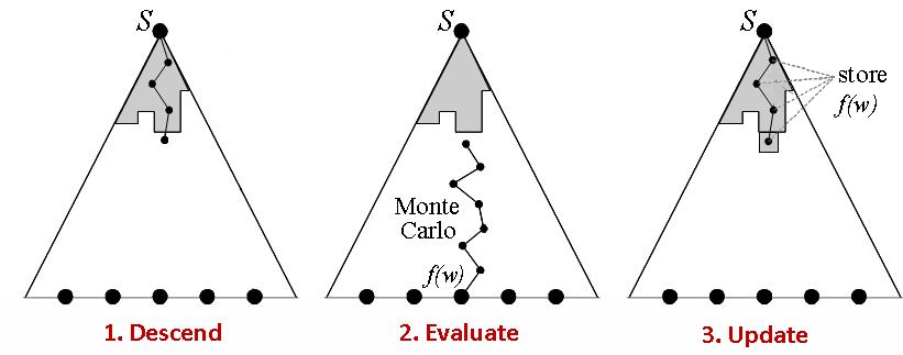
Figure 1: Monte-Carlo Tree Search: the tree is asymmetrically grown toward the most promising region (in grey, the known part of the tree). Each simulation is made of a MAB phase (1); then the simulation is completed until arriving at a final state (2); finally, the first node of the Monte-Carlo path is added to the known tree, and the reward is computed and back-propagated to all nodes of the path that are in the known tree (3).

4.1.3 Updating the tree

The number of visits of the nodes of the current tree that were in the path is incremented by 1; likewise, the cumulative reward associated to these nodes is incremented by the reward associated to the current path. Note that other statistics can be maintained in each node, such as the RAVE values [6], and must be updated there too.

4.2 Monte-Carlo Tree Schedule (MCS)

As already pointed out, solving a combinatorial problem can be viewed as a sequential decision making process, incrementally building a solution by choosing an element of a partial solution at a time (e.g., next town for TSP problems, of next machine to schedule for the job shop scheduling problem). In order to solve this sequential decision problem through a MCTS algorithm, several specific issues must be considered.

A first issue concerning the reward design has a significant impact on the exploration versus exploitation dilemma; it might require some instance-dependent parameter to reach a proper balance (see e.g., [21]). Indeed, in the case of job-shop scheduling for instance, different instances will have very different makespans.

A second issue concerns the heuristics to be used in the random phase (section 4.1.2). The original MCTS method [5] advocates pure random choices. Domain knowledge could however be used to propose a smarter procedure, e.g. using random selected dispatching rules for job-shop scheduling. Still, a lesson consistently learned from MCTS applications [6, 9] is that doing many simulations completed with a brute random phase is more effective than doing less simulations completed with a smart final phase. For instance in the domain of computer-Go, the overall results were degraded by using gnuGo in the random phase, compared to a uniform move selection. Likewise, the use of the three dispatching rules (described in Section 2) in the random phase was outperformed by a pure random strategy, uniformly selecting the next job to be considered. Here we have chosen to follow this path and our rollout phase consists of the purely random dispatching of jobs. Replacing this with line 2 in Algorithm 2, along with the $\varepsilon$–greedy policy, and the Pilot method is transformed into MCTS.

Another important detail must be taken into account: When performing random rollouts, we might forget the best choices found previously during the building of a schedule. For this reason, a global best found sequence is kept throughout the scheduling procedure. If a suboptimal choice is found in a later partial schedule ($k$-solution), the globally better choice previously found during a random rollout will be forced. In some sense the idea here is similar to that of the fortified rollouts used by the Pilot method [17].

Finally, in MCTS, the stopping criterion is defined by the total number of simulations (i.e., rollouts here), and one single decision is taken after a complete tree exploration, chosen as the child of the root node with the maximum expected reward [6]. The situation is rather different here, and, in this first approach to MCTS for combinatorial optimization, similarly to the Pilot method, a single tree exploration is done, with a limited budget in terms of number of rollouts. A complete schedule is then built by descending the tree and always choose the child with maximum expected reward (makespan).

5 Experimental Results

This section reports on the experimental validation of the proposed approaches. After detailing the experimental setting, the results of the MCS method is reported and compared to the baseline methods, the greedy application of the three dispatching rules MWKR, SPT and LOPN (section 2), and the pilot methods built on these three dispatching rules (section 3).

5.1 Experimental Settings

All experiments have been conducted using the set of test instances proposed in [22]. The machine orders for the jobs are randomly generated and the processing times are discrete values uniformly distributed between 1 and 200. Three different $n\times m$ problem sizes were generated using this setup, $6\times 6$, $10\times 10$ and $14\times 14$. The optimal makespans for one hundred instances generated of each size was then found using Brucker’s branch and bound algorithm [13]. A further four instance of size $20\times 20$ are also tested [23] and compared with their best known solution [24].

For all methods except the greedy ones, the time budget is varied to assess the convergence behavior of the pilot and MCS optimization methods, considering a total of 100, 1,000 and 5,000 rollouts a.k.a. simulation. Each rollout corresponds to designing and evaluating a complete solution (computing its total makespan). It is worth noting that not all rollouts are equally expensive; the rollout based on a dispatching rule (as used in the pilot methods) is more computationally demanding than the random rollout used in MCS, all the more so as the size of the problem instance increases. Nevertheless, the fixed rollout budget is meant to allow CPU-independent comparisons and assess the empirical behavior of the methods under restricted computational resources (e.g. in real-world situations).

For each method, each problem size and each time budget, the result is given as the average over 100 problem instances of the normalized makespan (1. being the optimal value), together with the minimum, maximum and median values, and the standard deviation; the number of times where the optimal value was found is additionally reported.

While the greedy and pilot algorithms actually are deterministic, MCS is not. The usual way to measure the performance of a stochastic algorithm on a given problem domain is through averaging the result out of a few dozen or hundred independent runs. For the sake of computational convenience however, MCS was run only once on each problem instance and the reported result is the average over the 100 independent instances.

5.2 The Greedy Algorithms

Instance	Heuristic	min	mean	median	stdev	max	#opt
$6\times 6$	MWKR	1.000	1.155	1.151	0.084	1.384	2
	SPT	1.137	1.399	1.390	0.150	1.816	0
	LOPN	1.017	1.176	1.178	0.083	1.369	0
$10\times 10$	MWKR	1.096	1.228	1.222	0.069	1.430	0
	SPT	1.303	1.654	1.644	0.166	2.161	0
	LOPN	1.103	1.216	1.208	0.061	1.369	0
$14\times 14$	MWKR	1.159	1.264	1.261	0.052	1.399	0
	SPT	1.584	2.012	2.015	0.244	2.721	0
	LOPN	1.150	1.253	1.250	0.048	1.376	0

Table 1: Greedy algorithms: Performance statistics of the MWKR, SPT and LOPN rules on three problem sizes.

The results of the greedy algorithms are depicted in Table 1 for the three dispatching rules MWKR, SPT and LOPN (section 2), showing that MWKR and LOPN behave similarly and significantly outperform SPT. Further, the performances of SPT significantly decrease with the problem size, whereas MWKR and LOPN demonstrate an excellent scalability in the considered size range.

Instance	Heuristic	min	mean	median	stdev	max	#opt
$6\times 6$	Pilot(MWKR,100)	1.000	1.049	1.050	0.038	1.167	14
	Pilot(MWKR,1000)	1.000	1.035	1.030	0.034	1.180	23
	Pilot(MWKR,5000)	1.000	1.025	1.014	0.029	1.104	33
	Pilot(SPT,100)	1.000	1.100	1.093	0.066	1.293	3
	Pilot(SPT,1000)	1.000	1.065	1.060	0.050	1.287	7
	Pilot(SPT,5000)	1.000	1.052	1.049	0.045	1.265	14
	Pilot(LOPN,100)	1.000	1.058	1.057	0.044	1.172	12
	Pilot(LOPN,1000)	1.000	1.046	1.036	0.040	1.134	17
	Pilot(LOPN,5000)	1.000	1.034	1.024	0.032	1.127	22
$10\times 10$	Pilot(MWKR,100)	1.032	1.109	1.109	0.039	1.217	0
	Pilot(MWKR,1000)	1.006	1.097	1.096	0.039	1.215	0
	Pilot(MWKR,5000)	1.004	1.082	1.083	0.035	1.158	0
	Pilot(SPT,100)	1.102	1.222	1.221	0.063	1.427	0
	Pilot(SPT,1000)	1.066	1.188	1.188	0.055	1.332	0
	Pilot(SPT,5000)	1.063	1.172	1.168	0.048	1.296	0
	Pilot(LOPN,100)	1.044	1.117	1.114	0.041	1.219	0
	Pilot(LOPN,1000)	1.028	1.106	1.105	0.042	1.212	0
	Pilot(LOPN,5000)	1.022	1.096	1.092	0.032	1.171	0
$14\times 14$	Pilot(MWKR,100)	1.081	1.156	1.155	0.036	1.256	0
	Pilot(MWKR,1000)	1.046	1.142	1.138	0.036	1.247	0
	Pilot(MWKR,5000)	1.046	1.129	1.129	0.034	1.230	0
	Pilot(SPT,100)	1.239	1.389	1.380	0.080	1.595	0
	Pilot(SPT,1000)	1.136	1.316	1.319	0.065	1.508	0
	Pilot(SPT,5000)	1.153	1.286	1.283	0.060	1.517	0
	Pilot(LOPN,100)	1.076	1.160	1.161	0.036	1.285	0
	Pilot(LOPN,1000)	1.080	1.149	1.152	0.037	1.264	0
	Pilot(LOPN,5000)	1.078	1.145	1.142	0.033	1.248	0

Table 2: Pilot algorithms. Performance statistics for Pilot algorithm using 3 different Pilot heuristics: MWKR, SPR, and LOPN, on the three different problem sizes.

5.3 The Pilot Method

The results of the pilot method (section 3) related to the three above dispatching rules and three time budgets (100, 1000 and 5000) are displayed in table 2 for all three problem sizes $6\times 6$, $10\times 10$, and $14\times 14$. For the sake of easy comparison with the greedy algorithm, the median performances respectively obtained on the same problem sizes displayed on Table 3.

As was expected, and demonstrated on some TSP instances by [3], the pilot method does improve on the greedy algorithm. With a time budget 100, a significant improvement is observed for all three methods, and confirmed by the number of times the optimal solution is discovered on problem size 6 x 6.

It is worth noting that the performance only very slightly improves when the time budget increases from 100 to 1000, and from 1000 to 5000, despite the significant increase in the computational effort. In particular, the optimal solutions are never discovered for higher problem sizes.

Lastly, the performance order of the three rules is not modified when using the pilot method: MWKR and LOPN significantly outperform SPT. As a consequence the Pilot method can be quite sensitive to the Pilot heuristic chosen.

Instance	Heuristic	Algorithm (budget)
			Pilot (100)	Pilot (1000)	Pilot (5000)
$6\times 6$	MWKR	1.151	1.050	1.030	1.014
	SPT	1.390	1.093	1.060	1.049
	LOPN	1.178	1.057	1.036	1.024
$10\times 10$	MWKR	1.222	1.109	1.096	1.083
	SPT	1.644	1.221	1.188	1.168
	LOPN	1.208	1.114	1.105	1.092
$14\times 14$	MWKR	1.261	1.155	1.138	1.129
	SPT	2.015	1.380	1.319	1.283
	LOPN	1.250	1.161	1.152	1.142

Table 3: Comparison of median performances of Greedy and Pilot with different budgets, for the 3 heuristics (from Tables 1 and 2).

5.4 Monte-Carlo Tree Schedule

Table 4 reports on the results of the MCS approach described in (section 4). On problem size 6x6, MCS significantly improves on the best Pilot method (MKWR with 5000 rollout budget), as also witnessed by the number of times the optimal solution is found. On problem size 10x10, the average and median performances are comparable; still, the optimal solution is found twice by MCS with a 5000 rollout budget, whereas it is never found by the Pilot method. On problem size 14x14, Pilot (MWKR,5000) is significantly better than MCS. A first explanation for this fact relies on the computational effort: As already mentioned, the computational time required for a 5,000 rollout Pilot is circa 4 times higher than for a 5,000 rollout MCS. A second explanation is the fact that, as the tree depth increases with the problem size, it becomes necessary to adjust the parameters controlling the branching factor of the MCS tree. This can be achieved by introducing progressive widening (on-going work).

Instance	Heuristic	min	mean	median	stdev	max	#opt
$6\times 6$
	MCS($\varepsilon$–greedy,100)	1.000	1.026	1.020	0.027	1.097	28
	MCS($\varepsilon$–greedy,1000)	1.000	1.014	1.001	0.025	1.150	50
	MCS($\varepsilon$–greedy,5000)	1.000	1.007	1.000	0.017	1.082	72
$10\times 10$
	MCS($\varepsilon$–greedy,100)	1.029	1.141	1.140	0.057	1.378	0
	MCS($\varepsilon$–greedy,1000)	1.014	1.095	1.098	0.036	1.199	0
	MCS($\varepsilon$–greedy,5000)	1.000	1.070	1.070	0.032	1.135	2
$14\times 14$
	MCS($\varepsilon$–greedy,100)	1.173	1.346	1.331	0.083	1.634	0
	MCS($\varepsilon$–greedy,1000)	1.127	1.284	1.280	0.074	1.552	0
	MCS($\varepsilon$–greedy,5000)	1.064	1.232	1.223	0.065	1.471	0

Table 4: Monte-Carlo Tree Schedule. Performance statistics using $\varepsilon$–greedy and random scheduling.

5.5 Larger Instances

The best known solutions (BKS) for the $20\times 20$ benchmark problem [23] are taken from [24]. Here we demonstrate the performance of the MCS on problems that cannot be solved using exact methods. Only four instances are considered here, and the MCS is run 30 times on each instance. The method is unable to find any best known solution. Nevertheless, the performance does not degrade significantly when compared to the results obtained on the $10\times 10$ problems.

Instance	Heuristic	min	mean	median	stdev	max	#BKS
yn01	MCS($\varepsilon$–greedy,100)	1.166	1.211	1.210	0.020	1.245	0
	MCS($\varepsilon$–greedy,1000)	1.144	1.186	1.183	0.021	1.235	0
	MCS($\varepsilon$–greedy,5000)	1.128	1.167	1.166	0.023	1.209	0
yn02	MCS($\varepsilon$–greedy,100)	1.135	1.185	1.181	0.024	1.228	0
	MCS($\varepsilon$–greedy,1000)	1.123	1.156	1.153	0.023	1.218	0
	MCS($\varepsilon$–greedy,5000)	1.090	1.130	1.130	0.023	1.174	0
yn03	MCS($\varepsilon$–greedy,100)	1.156	1.205	1.204	0.022	1.267	0
	MCS($\varepsilon$–greedy,1000)	1.131	1.178	1.180	0.020	1.222	0
	MCS($\varepsilon$–greedy,5000)	1.110	1.151	1.148	0.023	1.199	0
yn04	MCS($\varepsilon$–greedy,100)	1.063	1.108	1.107	0.025	1.160	0
	MCS($\varepsilon$–greedy,1000)	1.039	1.084	1.090	0.025	1.133	0
	MCS($\varepsilon$–greedy,5000)	1.023	1.067	1.064	0.019	1.102	0

Table 5: Results for the MCS on four $20\times 20$ instances. Performance statistics is given for 30 independent runs on each instance, yn01,$\ldots,$ yn04.

6 Discussion and Perspectives

The main contribution of this paper is to demonstrate the feasibility of using MCTS to address job-shop scheduling problems. This result has been obtained by using the simplest exploration/exploitation strategy in MCTS, the $\varepsilon$-greedy strategy, defining the Monte-Carlo Tree Scheduling approach (MCS). The empirical evidence gathered from the preliminary experiments presented here shows that MCS significantly outperforms its competitors on small and medium size problems. For larger problem sizes however, the Pilot method with the best dispatching rule outperforms this first verions of MCS. This fact is blamed on our adversary experimental setting, as we compared methods based on the number of rollouts, whereas the computational cost of a rollout is larger by almost an order of magnitude in the Pilot framework, as compared to that of the MCS.

The MCS scalability can also be improved through reconsidering the exploration vs exploitation trade-off, ever more critical in larger-sized problem instances. First of all, the MAX-k-arm strategy should be tried in lieu of the simple $\varepsilon$-greedy rule. Furthermore, this tradeoff can be also adjusted by avoiding the systematic first trial of all possible children, as this becomes harmful for large number or arms (jobs here). It is possible to control when a new child node should be added in the tree, and which one. Regarding the former aspect, a heuristics referred to as Progressive Widening has been designed to limit the branching factor of the tree, e.g. [10] . Regarding the second aspect, the use of a Rapid Action Value Estimate (RAVE), first developed in the computer-Go context [6] can be very efficient to aggregate the various rewards computed for the same option (Queen Elisabeth), and guide the introduction of the most efficient rules/jobs in average.

7 Conclusion and outlook

This work has shown how the Pilot method may be considered a special case of MCTS, with an exploratory-only strategy to traversing the tree and using a deterministic rollout driven by the Pilot heuristic. It has demonstrated that the Pilot method can be sensitive to the chosen Pilot heuristic. As the chosen Pilot heuristic becomes more effective, so too may its computational costs. An extension of the Pilot method in the realm of MCTS algorithms, the MCS, has been proposed, using a simple $\epsilon$–greedy strategy to traverse down the tree. However, more sophisticated strategies, such as the one based on the max-$k$ bandit problem [12, 20], need now be investigated. For larger problems, progressive widening should be an avenue for further research, as similar strategies have already been investigated in the Pilot framework. Finally, Rapid Action Value Estimates may not only be used to bias how the tree is traversed, possibly replacing the exploration term in the bandit formulas, but can also help to improve over the random rollouts.

References

- [1] Xu, L., Hutter, F., Hoos, H.H., Leyton-Brown, K.: Satzilla: Portfolio-based algorithm selection for sat. Journal of Artificial Intelligence Research 32 (2008) 565–606
- [2] Burke, E., Hyde, M., Kendall, G., Ochoa, G., Ozcan, E., Qu, R.: Hyper-heuristics: A Survey of the State of the Art. Technical report, NOTTCS-TR-SUB-0906241418-2747, University of Nottingham (2010) http://www.cs.nott.ac.uk/~gxo/papers/hhsurvey.pdf.
- [3] Duin, C., Voß, S.: The Pilot method: A strategy for heuristic repetition with application to the Steiner problem in graphs. Networks 34(3) (October 1999) 181–191
- [4] Lagoudakis, M.G., Parr, R.: Reinforcement learning as classification: Leveraging modern classifiers. In Fawcett, T., Mishra, N., eds.: Proc. 20th Int. Conf. on Machine Learning (ICML’03), AAAI Press (2003) 424–431
- [5] Kocsis, L., Szepesvári, C.: Bandit based monte-carlo planning. In Fürnkranz, J., Scheffer, T., Spiliopoulou, M., eds.: Proc. Eur. Conf. on Machine Learning (ECML’06), LNCS 4112, Springer Verlag (2006) 282–293
- [6] Gelly, S., Silver, D.: Combining online and offline knowledge in uct. In: Proc. of the 24th Int. Conf. on Machine learning (ICML’07), ACM Press (2007) 273–280
- [7] Asmuth, J., Littman, M.: Learning is planning: near Bayes-optimal reinforcement learning via Monte-Carlo tree search. In: Proceedings of The 27th Conference on Uncertainty in Artificial Intelligence (UAI-11). (2011)
- [8] Lai, T., Robbins, H.: Asymptotically efficient adaptive allocation rules. Advances in Applied Mathematics 6 (1985) 4–22
- [9] De Mesmay, F., Rimmel, A., Voronenko, Y., Püschel, M.: Bandit-Based Optimization on Graphs with Application to Library Performance Tuning. In Danyluk, A., Bottou, L., Littman, M., eds.: Proc. Int. Conf. on Machine Learning (ICML’09). Volume 382 of ACM International Conference Proceeding Series., ACM (2009) 729–736
- [10] Rolet, P., Sebag, M., Teytaud, O.: Boosting active learning to optimality: A tractable monte-carlo, billiard-based algorithm. In Wray L. Buntine et al., ed.: Proc. ECML/PKDD, LNCS 5782, Springer Verlag (2009) 302–317
- [11] Matsumoto, S., Hirosue, N., Itonaga, K., Ueno, N., Ishii, H.: Monte-Carlo Tree Search for a reentrant scheduling problem. In: 40th Intl Conf. on Computers and Industrial Engineering (CIE’10), IEEE (2010) 1–6
- [12] Streeter, M., Smith, S.: A simple distribution-free approach to the max k-armed bandit problem. Principles and Practice of Constraint Programming (CP’06) 4204(2006) (2006) 560–574
- [13] Brucker, P.: Scheduling algorithms. Springer (2007)
- [14] Bräsel, H., Dornheim, L., Kutz, S., Mörig, M., Rössling, I.: LiSA – Library of Scheduling Algorithms. Otto-von-Guericke Universität Magdeburg. (2011) http://lisa.math.uni-magdeburg.de.
- [15] Panwalkar, S., Iskander, W.: A Survey of Scheduling Rules. Operations Research 25(1) (1977) 45–61
- [16] Kawai, T., Fujimoto, Y.: An efficient combination of dispatch rules for job-shop scheduling problem. 3rd IEEE Intl Conf. on Industrial Informatics (INDIN’05) (2005) 484–488
- [17] Voß, S., Fink, A., Duin, C.: Looking ahead with the pilot method. Annals of Operations Research 136(1) (2005) 285–302
- [18] Bertsekas, D., Tsitsiklis, J., Wu, C.: Rollout algorithms for combinatorial optimization. Journal of Heuristics 3(3) (1997) 245–262
- [19] Auer, P., Cesa-Bianchi, N., Fischer, P.: Finite-time analysis of the multiarmed bandit problem. Machine Learning 47(2-3) (2002) 235–256
- [20] Cicirello, V., Smith, S.: The max k-armed bandit: A new model of exploration applied to search heuristic selection. In Veloso, M.M., Kambhampati, S., eds.: Proc. Nat. Conf. on Artificial Intelligence, AAAI Press / The MIT Press (2005) 1355–1361
- [21] Fialho, A., Da Costa, L., Schoenauer, M., Sebag, M.: Dynamic multi-armed bandits and extreme value-based rewards for adaptive operator selection in evolutionary algorithms. In T. Stuetzle et al., ed.: Proc. 3rd Intl Conf. on Learning and Intelligent OptimizatioN (LION’09), LNCS 5851Springer Verlag (2009) 176–190
- [22] Taillard, E.: Benchmarks for basic scheduling problems. European Journal of Operational Research 64(2) (1993) 278–285
- [23] Yamada, T.., Nakano, R.: A genetic algorithm applicable to large-scale job shop Problems. In Reinhard Männer and Bernard Manderick, ed.: Parallel Problem Solving from Nature (PPSN II), Elsevier (1992) 283–292
- [24] Banharnsakun, A., Sirinaovakul, B., Achalakul, T.: Job Shop Scheduling with the Best-so-far ABC. Engineering Applications of Artificial Intelligence (2006) (2011) 1–11